Hook-length formulas for skew shapes
32
HOOK FORMULAS FOR SKEW SHAPES II. COMBINATORIAL PROOFS AND ENUMERATIVE APPLICATIONS ALEJANDRO H. MORALES ? , IGOR PAK ? , AND GRETA PANOVA † Abstract. The Naruse hook-length formula is a recent general formula for the number of stan- dard Young tableaux of skew shapes, given as a positive sum over excited diagrams of products of hook-lengths. In [MPP1] we gave two different q-analogues of Naruse’s formula: for the skew Schur functions, and for counting reverse plane partitions of skew shapes. In this paper we give an elemen- tary proof of Naruse’s formula based on the case of border strips. For special border strips, we obtain curious new formulas for the Euler and q-Euler numbers in terms of certain Dyck path summations. 1. Introduction In Enumerative Combinatorics, when it comes to fundamental results, one proof is rarely enough, and one is often on the prowl for a better, more elegant or more direct proof. In fact, there is a wide belief in multitude of “proofs from the Book”, rather than a singular best approach. The reasons are both cultural and mathematical: different proofs elucidate different aspects of the underlying combinatorial objects and lead to different extensions and generalizations. The story of this series of papers is on our effort to understand and generalize the Naruse hook- length formula (NHLF) for the number of standard Yound tableaux of a skew shape in terms of excited diagrams. In our previous paper [MPP1], we gave two q-analogues of the NHLF, the first with an algebraic proof and the second with a bijective proof. We also gave a (difficult) “mixed” proof of the first q-analogue, which combined the bijection with an algebraic argument. Naturally, these provided new proofs of the NHLF, but none which one would call “elementary”. This paper is the second in the series. Here we consider a special case of border strips which turn out to be extremely fruitful both as a technical tool and as an important object of study. We give two elementary proofs of the NHLF in this case, both inductive: one using weighted paths argument and another using determinant calculation. We then deduce the general case of NHLF for all skew diagrams by using the Lascoux–Pragacz identity for Schur functions. Since the latter has its own elementary proof [HaG] (see also [CYY]), we obtain an elementary proof of the HLF. But surprises do not stop here. For the special cases of the zigzag strips, our approach gives a number of curious new formulas for the Euler and and two types of q-Euler numbers, the second of which seems to be new. Because the excited diagrams correspond to Dyck paths in this case, the resulting summations have Catalan number terms. We also give type B analogues, which have similar feel but with ( 2n n ) terms. Despite their strong “classical feel” all these formulas are new and quite mysterious. 1.1. Hook formulas for straight and skew shapes. Let us recall the main result from the first paper [MPP1] in this series. We assume here the reader is familiar with the basic definitions, which are postponed until the next two sections. Key words and phrases. Hook-length formula, excited tableau, standard Young tableau, flagged tableau, reverse plane partition, alternating permutation, Dyck path, Euler numbers, Catalan numbers, factorial Schur function. March 22, 2017. ? Department of Mathematics, UCLA, Los Angeles, CA 90095. Email: {ahmorales, pak}@math.ucla.edu. † Department of Mathematics, UPenn, Philadelphia, PA 19104. Email: [email protected]. 1
Transcript of Hook-length formulas for skew shapes

HOOK FORMULAS FOR SKEW SHAPES II. COMBINATORIAL PROOFS
AND ENUMERATIVE APPLICATIONS
ALEJANDRO H. MORALES?, IGOR PAK?, AND GRETA PANOVA†
Abstract. The Naruse hook-length formula is a recent general formula for the number of stan-dard Young tableaux of skew shapes, given as a positive sum over excited diagrams of products of
hook-lengths. In [MPP1] we gave two different q-analogues of Naruse’s formula: for the skew Schurfunctions, and for counting reverse plane partitions of skew shapes. In this paper we give an elemen-
tary proof of Naruse’s formula based on the case of border strips. For special border strips, we obtain
curious new formulas for the Euler and q-Euler numbers in terms of certain Dyck path summations.
1. Introduction
In Enumerative Combinatorics, when it comes to fundamental results, one proof is rarely enough,and one is often on the prowl for a better, more elegant or more direct proof. In fact, there is a widebelief in multitude of “proofs from the Book”, rather than a singular best approach. The reasonsare both cultural and mathematical: different proofs elucidate different aspects of the underlyingcombinatorial objects and lead to different extensions and generalizations.
The story of this series of papers is on our effort to understand and generalize the Naruse hook-length formula (NHLF) for the number of standard Yound tableaux of a skew shape in terms ofexcited diagrams. In our previous paper [MPP1], we gave two q-analogues of the NHLF, the first withan algebraic proof and the second with a bijective proof. We also gave a (difficult) “mixed” proofof the first q-analogue, which combined the bijection with an algebraic argument. Naturally, theseprovided new proofs of the NHLF, but none which one would call “elementary”.
This paper is the second in the series. Here we consider a special case of border strips which turnout to be extremely fruitful both as a technical tool and as an important object of study. We givetwo elementary proofs of the NHLF in this case, both inductive: one using weighted paths argumentand another using determinant calculation. We then deduce the general case of NHLF for all skewdiagrams by using the Lascoux–Pragacz identity for Schur functions. Since the latter has its ownelementary proof [HaG] (see also [CYY]), we obtain an elementary proof of the HLF.
But surprises do not stop here. For the special cases of the zigzag strips, our approach gives anumber of curious new formulas for the Euler and and two types of q-Euler numbers, the second ofwhich seems to be new. Because the excited diagrams correspond to Dyck paths in this case, theresulting summations have Catalan number terms. We also give type B analogues, which have similarfeel but with
(2nn
)terms. Despite their strong “classical feel” all these formulas are new and quite
mysterious.
1.1. Hook formulas for straight and skew shapes. Let us recall the main result from the firstpaper [MPP1] in this series. We assume here the reader is familiar with the basic definitions, whichare postponed until the next two sections.
Key words and phrases. Hook-length formula, excited tableau, standard Young tableau, flagged tableau, reverse
plane partition, alternating permutation, Dyck path, Euler numbers, Catalan numbers, factorial Schur function.March 22, 2017.?Department of Mathematics, UCLA, Los Angeles, CA 90095. Email: {ahmorales,pak}@math.ucla.edu.†Department of Mathematics, UPenn, Philadelphia, PA 19104. Email: [email protected].
1
2 ALEJANDRO MORALES, IGOR PAK, GRETA PANOVA
The standard Young tableaux (SYT) of straight and skew shapes are central objects in enumerativeand algebraic combinatorics. The number fλ = |SYT(λ)| of standard Young tableaux of shape λ hasthe celebrated hook-length formula (HLF):
Theorem 1.1 (HLF; Frame–Robinson–Thrall [FRT]). Let λ be a partition of n. We have:
(HLF) fλ =n!∏
u∈[λ] h(u),
where h(u) = λi − i+ λ′j − j + 1 is the hook-length of the square u = (i, j).
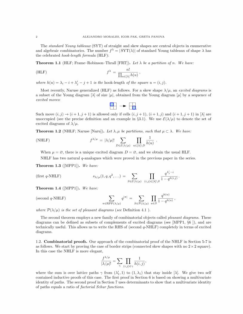
Most recently, Naruse generalized (HLF) as follows. For a skew shape λ/µ, an excited diagrams isa subset of the Young diagram [λ] of size |µ|, obtained from the Young diagram [µ] by a sequence ofexcited moves:
.
Such move (i, j)→ (i+ 1, j + 1) is allowed only if cells (i, j + 1), (i+ 1, j) and (i+ 1, j + 1) in [λ] areunoccupied (see the precise definition and an example in §3.1). We use E(λ/µ) to denote the set ofexcited diagrams of λ/µ.
Theorem 1.2 (NHLF; Naruse [Naru]). Let λ, µ be partitions, such that µ ⊂ λ. We have:
(NHLF) fλ/µ = |λ/µ|!∑
D∈E(λ/µ)
∏u∈[λ]\D
1
h(u).
When µ = ∅, there is a unique excited diagram D = ∅, and we obtain the usual HLF.
NHLF has two natural q-analogues which were proved in the previous paper in the series.
Theorem 1.3 ([MPP1]). We have:
(first q-NHLF) sλ/µ(1, q, q2, . . .) =∑
S∈E(λ/µ)
∏(i,j)∈[λ]\S
qλ′j−i
1− qh(i,j).
Theorem 1.4 ([MPP1]). We have:
(second q-NHLF)∑
π∈RPP(λ/µ)
q|π| =∑
S∈P(λ/µ)
∏u∈S
qh(u)
1− qh(u),
where P(λ/µ) is the set of pleasant diagrams (see Definition 4.1 ).
The second theorem employs a new family of combinatorial objects called pleasant diagrams. Thesediagrams can be defined as subsets of complements of excited diagrams (see [MPP1, §6 ]), and aretechnically useful. This allows us to write the RHS of (second q-NHLF) completely in terms of exciteddiagrams.
1.2. Combinatorial proofs. Our approach of the combinatorial proof of the NHLF in Section 5-7 isas follows. We start by proving the case of border strips (connected skew shapes with no 2×2 square).In this case the NHLF is more elegant,
fλ/µ
|λ/µ|! =∑γ
∏(i,j)∈γ
1
h(i, j),
where the sum is over lattice paths γ from (λ′1, 1) to (1, λ1) that stay inside [λ]. We give two selfcontained inductive proofs of this case. The first proof in Section 6 is based on showing a multivariateidentity of paths. The second proof in Section 7 uses determinants to show that a multivariate identityof paths equals a ratio of factorial Schur functions.
HOOK FORMULAS FOR SKEW SHAPES II 3
We then use a corollary of the Lascoux–Pragacz identity for skew Schur functions: if (θ1, . . . , θk) isa decomposition of the shape λ/µ into outer border strips θi (see Section 7.5) then
fλ/µ
|λ/µ|! = det
[fθi#θj
|θi#θj |!
]ki,j=1
,
where θi#θj is a certain substrip of the outer border strip of λ.Combining the case for border strips and this determinantal identity we get
fλ/µ
|λ/µ|! = det
∑γ:(aj ,bj)→(ci,di),
γ⊆λ
∏(r,s)∈γ
1
h(r, s)
k
i,j=1
,
where (aj , bj) and (ci, di) are the endpoints of the border strip θi#θj . Lastly, using the Lindstrom–Gessel–Viennot lemma this determinant is written as a weighted sum over non-intersecting latticepaths in λ. By an explicit characterization of excited diagrams in Section 3, the supports of suchpaths are exactly the complements of excited diagrams. The NHLF then follows.
A similar approach is used in Section 5 to give a combinatorial proof of the first q-NHLF for allskew shapes given in [MPP1]. The Hillman–Grassl inspired bijection in [MPP1] remains the onlycombinatorial proof of the second q-NHLF.
Remark 1.5. We should mention that our inductive proof is involutive, but basic enough to allow“bijectification”, i.e. an involution principle proof of the NHLF. We refer to [K1, Rem, Zei] for theinvolution principle proofs of the (usual) HLF.
1.3. Enumerative applications. In sections 8 and 9, we give enumerative formulas which followfrom NHLF. They involve q-analogues of Catalan, Euler and Schroder numbers. We highlight severalof these formulas.
Let Alt(n) = {σ(1) < σ(2) > σ(3) < σ(4) > . . .} ⊂ Sn be the set of alternating permutations. Thenumber En = |Alt(n)| is the n-th Euler number (see [S3] and [OEIS, A000111]), with the g.f.
(1.1) 1 +
∞∑n=1
Enxn
n!= tan(x) + sec(x) .
Let δn = (n−1, n−2, . . . , 2, 1) denotes the staircase shape and observe that E2n+1 = fδn+2/δn . Thus,the NHLF relates Euler numbers with excited diagrams of δn+2/δn. It turns out that these exciteddiagrams are in correspondence with the set Dyck(n) of Dyck paths of length 2n (see Corollary 8.1).More precisely,
|E(δn+2/δn)| = |Dyck(n)| = Cn =1
n+ 1
(2n
n
),
where Cn is the n-th Catalan number, and Dyck(n) is the set of lattice paths from (0, 0) to (2n, 0)with steps (1, 1) and (1,−1) that stay on or above the x-axis (see e.g. [S5]). Now the NHLF impliesthe following identity.
Corollary 1.6. We have:
(EC)∑
p∈Dyck(n)
∏(a,b)∈p
1
2b+ 1=
E2n+1
(2n+ 1)!,
where (a, b) ∈ p denotes a point (a, b) of the Dyck path p.
Consider the following two q-analogues of En :
En(q) :=∑
σ∈Alt(n)
qmaj(σ−1) and E∗n(q) :=∑
σ∈Alt(n)
qmaj(σ−1κ) ,

4 ALEJANDRO MORALES, IGOR PAK, GRETA PANOVA
where maj(σ) is the major index of permutation σ in Sn and κ is the permutation κ = (13254 . . .).See examples 8.6 and 9.5 for the initial values.
Now, for the skew shape δn+2/δn, Theorem 1.3 gives the following q-analogue of Corollary 1.6.
Corollary 1.7. We have:∑p∈Dyck(n)
∏(a,b)∈p
qb
1− q2b+1=
E2n+1(q)
(1− q)(1− q2) · · · (1− q2n+1).
Similarly, Theorem 1.4 in this case gives a different q-analogue.
Corollary 1.8. We have:∑p∈Dyck(n)
qH(p)∏
(a,b)∈p
1
1− q2b+1=
E∗2n+1(q)
(1− q)(1− q2) · · · (1− q2n+1),
where
H(p) =∑
(c,d)∈HP(p)
(2d+ 1) ,
and HP(p) denotes the set of peaks (c, d) in p with height d > 1.
All three corollaries are derived in sections 8 and 9.
Section 8 considers the special case when λ/µ is a thick strip shape δn+2k/δn, which give theconnection with Euler and Catalan numbers. In Section 9, we consider the pleasant diagrams of thethick strip shapes, establishing connection with Schroder numbers. We also state conjectures on certaindeterminantal formulas. We conclude with final remarks and open problems in Section 10.
2. Notation and Background
2.1. Young diagrams. Let λ = (λ1, . . . , λr), µ = (µ1, . . . , µs) denote integer partitions of length`(λ) = r and `(µ) = s. The size of the partition is denoted by |λ| and λ′ denotes the conjugate partitionof λ. We use [λ] to denote the Young diagram of the partition λ. The hook length hij = λi−i+λ′j−j+1of a square u = (i, j) ∈ [λ] is the number of squares directly to the right and directly below u in [λ].The Durfee square �λ is the largest square inside [λ]; it is always of the form {(i, j), 1 ≤ i, j ≤ k}.
A skew shape is denoted by λ/µ. A skew shape can have multiple edge connected components. Foran integer k, 1 − `(λ) ≤ k ≤ λ1 − 1, let dk be the diagonal {(i, j) ∈ λ/µ | i − j = k}, where µk = 0if k > `(µ). For an integer t, 1 ≤ t ≤ `(λ) − 1 let dt(µ) denote the diagonal dµt−t where µt = 0 if`(µ) < t ≤ `(λ).
Given the skew shape λ/µ, let Pλ/µ be the poset of cells (i, j) of [λ/µ] partially ordered by compo-nent. This poset is naturally labelled, unless otherwise stated.
2.2. Young tableaux. A reverse plane partition of skew shape λ/µ is an array π = (πij) of non-negative integers of shape λ/µ that is weakly increasing in rows and columns. We denote the set ofsuch plane partitions by RPP(λ/µ). A semistandard Young tableau of shape λ/µ is a RPP of shapeλ/µ that is strictly increasing in columns. We denote the set of such tableaux by SSYT(λ/µ). Astandard Young tableau (SYT) of shape λ/µ is an array T of shape λ/µ with the numbers 1, . . . , n,where n = |λ/µ|, each i appearing once, strictly increasing in rows and columns. For example, thereare five SYT of shape (32/1):
1 23 4
1 32 4
1 42 3
2 31 4
2 41 3
The size of a RPP or tableau T is the sum of its entries. A descent of a SYT T is an index i such thati+ 1 appears in a row below i. The major index tmaj(T ) is the sum
∑i over all the descents of T .
HOOK FORMULAS FOR SKEW SHAPES II 5
2.3. Skew Schur functions. Let sλ/µ(x) denote the skew Schur function of shape λ/µ in variablesx = (x0, x1, x2, . . .). In particular,
sλ/µ(x) =∑
T∈SSYT(λ/µ)
xT , sλ/µ(1, q, q2, . . .) =∑
T∈SSYT(λ/µ)
q|T | ,
where xT = x#0s in (T )0 x
#1s in (T )1 . . . Recall, the skew shape λ/µ can have multiple edgewise connected
components θ1, . . . , θm. Since then sλ/µ = sθ1 · · · sθk we assume without loss of generality that λ/µ isedgewise connected.
2.4. Determinantal identities for sλ/µ. The Jacobi-Trudi identity (see e.g. [S4, §7.16]) states that
(2.1) sλ/µ(x) = det[hλi−µj−i+j(x)
]ni,j=1
,
where hk(x) =∑i1≤i2≤···≤ik xi1xi2 · · ·xik is the k-th complete symmetric function.
There are other determinantal identities of (skew) Schur functions like the Giambelli formula (e.g.see [S4, Ex. 7.39]) and the Lascoux–Pragacz identity [LasP]. Hamel and Goulden [HaG] found a vastcommon generalization to these three identities by giving an exponential number of determinantalidentities for sλ/µ depending on outer decompositions of the shape λ/µ. We focus on the Lascoux–Pragacz identity that we describe next through the Hamel–Goulden theory (e.g. see [CYY]).
A border strip is a connected skew shape without any 2× 2 squares. The starting point and endingpoint of a strip are its southeast and northeast endpoints. Given λ, the outer border strip is the stripcontaining all the boxes sharing a vertex with the boundary of λ., i.e. λ/(λ2 − 1, λ3 − 1, . . .). ALascoux–Pragacz decomposition of λ/µ is a decomposition of the skew shape into k maximal outerborder strips (θ1, . . . , θk), where θ1 is the outer border strip of λ, θ2 is the outer border strip of theremaining diagram λ \ θ1, and so on until we start intersecting µ. In this case, we continue thedecomposition with each remaining connected component. The strips are ordered � by the contentsof their northeast endpoints. See Figure 2.4, left, for an example.
We call the border strip θ1 the cutting strip of the decomposition and denote it by τ [CYY]. Forintegers p and q, let φ[p, q] be the substrip of τ consisting of the cells with contents between p and q.By convention, θ[p, p] = (1), φ[p+ 1, p] = ∅ and φ[p, q] with p > q+ 1 is undefined. The strip θi#θj isthe substrip φ[p(θj), q(θi)] of τ , where p(θi) and q(θi) are the contents of the starting point and endingpoint of θi.
Theorem 2.1 (Lascoux–Pragacz [LasP], Hamel–Goulden [HaG]). If (θ1, . . . , θk) is a Lascoux–Pragaczdecomposition of λ/µ, then
(2.2) sλ/µ = det[sθi#θj
]ki,j=1
.
where s∅ = 1 and sφ[p,q] = 0 if φ[p, q] is undefined.
Example 2.2. Figure 2.4, right, shows the Lascoux–Pragacz decomposition for the shape λ/µ =(5441/21) into two strips (θ1, θ2). Then τ = θ1 = (5441/33) and
θ1#θ1 = θ1, θ1#θ2 = φ[0, 4] = (322/11), θ2#θ1 = φ[−3, 2] = (441/3), θ2#θ2 = θ2.
Then by the Lascoux–Pragacz identity s(5441/21) can be written as the following 2× 2 determinant
sλ/µ = det
[sθ1#θ1 sθ1#θ2
sθ2#θ1 sθ2#θ2
]= det
[s5441/33 s322/11
s441/3 s22/1
].
2.5. Factorial Schur functions. The factorial Schur function (e.g. see [MS]) is defined as
s(d)µ (x | a) :=
det[(xi − a1) · · · (xi − aµj+d−j)
]di,j=1∏
1≤i<j≤d(xi − xj)
,
where x = x1, . . . , xd and a = a1, a2, . . . is a sequence of parameters.

6 ALEJANDRO MORALES, IGOR PAK, GRETA PANOVA
θ1θ2θ3θ4
θ5
Figure 1. Left: Example of a Lascoux–Pragacz outer decomposition. Right: theLascoux–Pragacz decomposition of the shape λ/µ = (5441/21) and the border stripsof the determinantal identity for sλ/µ
2.6. Permutations. We write permutations of {1, 2, . . . , n} in one-line notation: w = (w1w2 . . . wn)where wi is the image of i. A descent of w is an index i such that wi > wi+1. The major index maj(w)is the sum
∑i of all the descents i of w.
2.7. Dyck paths. A Dyck path p of length 2n is a lattice paths from (0, 0) to (2n, 0) with steps (1, 1)and (1,−1) that stay on or above the x-axis. We use Dyck(n) to denote the set of Dyck paths oflength 2n. For a Dyck path p, a peak is a point (c, d) such that (c − 1, d − 1) and (c + 1, d − 1) ∈ p.Peak (c, d) is called a high-peak if d > 1.
3. Excited diagrams
3.1. Definition. Let λ/µ be a skew partition and D be a subset of the Young diagram of λ. A cellu = (i, j) ∈ D is called active if (i + 1, j), (i, j + 1) and (i + 1, j + 1) are all in [λ] \D. Let u be anactive cell of D, define αu(D) to be the set obtained by replacing (i, j) in D by (i+ 1, j + 1). We callthis replacement an excited move. An excited diagram of λ/µ is a subdiagram of λ obtained from theYoung diagram of µ after a sequence of excited moves on active cells. Let E(λ/µ) be the set of exciteddiagrams of λ/µ and e(λ/µ) its cardinality. For example, Figure 2 shows the eight excited diagramsof (5441/21) (for the moment ignore the paths in the complement).
Figure 2. The eight excited diagrams (in blue) of shape λ/µ = (5441/21) and thecorresponding non-intersecting paths (in red) in their complement. The high peaksof the paths described in Section 4.1 are in gray.
3.2. Flagged tableaux. Excited diagrams of λ/µ are equivalent to certain flagged tableaux of shape µ(see [MPP1, §3] and [Kre1, §6]). Thus, the number of excited diagrams is given by a determinant, apolynomial in the parts of λ and µ as follows. Consider the diagonal that passes through cell (i, µi),
i.e. the last cell of row i in µ. Let this diagonal intersect the boundary of λ at a row denoted by f(λ/µ)i .

HOOK FORMULAS FOR SKEW SHAPES II 7
Proposition 3.1 ([MPP1]). In notation above, we have:
e(λ/µ) = det
[(f(λ/µ)i + µi − i+ j − 1
f(λ/µ)i − 1
)]`(µ)
i,j=1
.
Example 3.2. For the same shape as in Example 2.2 and Figure 2, the number of excited diagramsequals the number of flagged tableaux of shape (2, 1) with entries in the first and second row ≤ 2.Thus
e(λ/µ) = det
[(42
) (52
)(22
) (32
)] = det
[6 101 3
]= 8.
3.3. Border strip decomposition formula for e(λ/µ). This first determinantal identity for e(λ/µ)is similar to the Jacobi–Trudi identity for sµ. In this section we prove a new determinantal identityfor e(λ/µ) very similar to the Lascoux–Pragacz identity for sλ/µ.
Theorem 3.3. If (θ1, . . . , θk) is the Lascoux–Pragacz decomposition of λ/µ into k maximal outerborder strips then
e(λ/µ) = det[e(θi#θj)
]ki,j=1
,
where e(∅) = 1 and e(φ[p, q]) = 0 if φ[p, q] is undefined.
Example 3.4. For the same shape λ/µ as in Example 2.2 and Figure 2 we have
e(λ/µ) = det
[e(5441/33) e(322/11)e(441/3) e(22/1)
]= det
[10 34 2
]= 8.
In order to prove Theorem 3.3 we show a relation between excited diagrams and certain tuples ofnon-intersecting paths.
For the connected skew shape λ/µ there is a unique tuple of border-strips (i.e. non-intersectingpaths) γ∗1 , . . . , γ
∗k in λ with support [λ/µ], where each border strip γ∗i begins at the southern box
(a′i, b′i) of a column and ends at the eastern box (c′i, d
′i) of a row [Kre1, Lemma 5.3]. We call this
tuple the Kreiman decomposition of λ/mu. Let NI(λ/µ) be the set of k-tuples Γ := (γ1, . . . , γk)of non-intersecting paths contained in [λ] with γi : (ai, bi) → (ci, di). The supports of the paths inNI(λ/µ) are exactly the complements of excited diagrams in E(λ/µ) [Kre1, §5.5]. See Figure 2, foran example.
Proposition 3.5 (Kreiman [Kre1]). The k-tuples of paths in NI(λ/µ) are uniquely determined bytheir support in [λ] and moreover these supports are exactly the complements of excited diagramsof λ/µ.
Proof. The fact that paths are uniquely determined by their support in [λ] follows by [Kre1, Lemma5.2]. By abuse of notation we identify the k-tuples of paths in NI(λ/µ) with their supports. Notethat the supports of all k-tuples of paths in NI(λ/µ) have size |λ/µ|.
We now show that the support of k-tuples in NI(λ/µ) correspond to complements of exciteddiagrams.
First, we show that if D ∈ E(λ/µ) then [λ] \D ∈ NI(λ/µ) by induction on the number of excitedmoves. Given [µ] ∈ E(λ/µ), its complement [λ/µ] corresponds to Kreiman decomposition (γ∗1 , . . . , γ
∗k) ∈
NI(λ/µ) as mentioned above. Then excited moves on the diagrams correspond to ladder moves onthe non-intersecting paths:
.
The latter do not introduce intersections and preserve the endpoints of the paths. Thus for eachD ∈ E(λ/µ), its complement [λ] \D corresponds to a k-tuple (γ1, . . . , γk) of paths in NI(λ/µ).

8 ALEJANDRO MORALES, IGOR PAK, GRETA PANOVA
θ1θ2θ3θ4
θ5
γ∗1
γ∗2
γ∗3
γ∗4
γ∗5
Figure 3. Example of the correspondence of the border strips of the Lascoux–Pragacz outer decomposition (θ1, . . . , θ5) and Kreiman outer decomposition(γ∗1 , . . . , γ
∗5 ) of λ/µ. The contents of the endpoints and the lengths of θi and γ∗i
are the same.
Conversely, consider the support S of a k-tuple of paths in NI(λ/µ). The set S has the followingproperty: the subset Sk := S ∩�λk has no descending chain bigger than the length of the kth diagonalof λ/µ. Such sets S are called pleasant diagram of λ/µ [MPP1, §6] (see Section 4). Since |S| = |λ/µ|,by [MPP1, Thm. 6.5] the set S is the complement of an excited diagram in E(λ/µ), as desired. �
Corollary 3.6. e(λ/µ) = |NI(λ/µ)|.Next, we show a correspondence between the Kreiman decomposition and the Lascoux–Pragacz
decomposition of λ/µ.
Lemma 3.7. There is a correspondence between the border strips of the Lascoux–Pragacz and theKreiman decomposition of λ/µ that preserves the lengths and contents of the starting and endingpoints of the paths/border strips:
p(θi) = bi − ai, q(θi) = di − ci.Proof. Let (θ1, . . . , θk) and (γ∗1 , . . . , γ
∗t ) be the Lascoux–Pragacz and the Kreiman decomposition of
the shape λ/µ. We prove the result by induction on k. Note that θ1 and γ∗1 have the same endpoints(λ′1, 1) and (1, λ1). Thus the strips have the same length and their endpoints have the same respectivecontents.
Next, note that the skew shapes λ/µ with θ1 removed and λ/µ with γ∗1 removed are the same. TheLascoux–Pragacz of this new shape is (θ2, . . . , θk) with the contents of the endpoints unchanged. Sim-ilarly, the Kreiman decomposition of this new shape is (γ∗2 , . . . , γ
∗t ) with the contents of the endpoints
unchanged. By induction k − 1 = t− 1 and the strip θi and γ∗i for i = 2, . . . , k have the same lengthand their endpoints have the same content. This completes the proof. �
Lastly, we need a Lindstrom–Gessel–Viennot type Lemma to count (weighted) non-intersectingpaths in [λ]. To state the Lemma we need some notation. Its proof follows the usual sign-reversinginvolution on paths that intersect (e.g. see [S4, §2.7]). Let (a1, b1), . . . , (ak, bk) and (c1, d1), . . . , (ck, dk)be cells in [λ] and let
h((aj , bj)→ (ci, di),y) :=∑γ
∏(r,s)∈γ
yr,s,
where the sum is over paths γ : (aj , bj)→ (ci, di) in [λ] with steps (1, 0) and (0, 1), and the product isover cells (r, s) of γ. Let also
Nλ((ai, bi)→ (ci, di); y) :=∑
(γ1,...,γk)
k∏i=1
∏(r,s)∈γi
yr,s,
where the sum is over k-tuples (γ1, . . . , γk) of non-intersecting paths γi : (ai, bi)→ (ci, di) in [λ].
Lemma 3.8 (Lindstrom–Gessel–Viennot).
Nλ((ai, bi)→ (ci, di),y) = det[h((aj , bj)→ (ci, di),y)
]ki,j=1
.
HOOK FORMULAS FOR SKEW SHAPES II 9
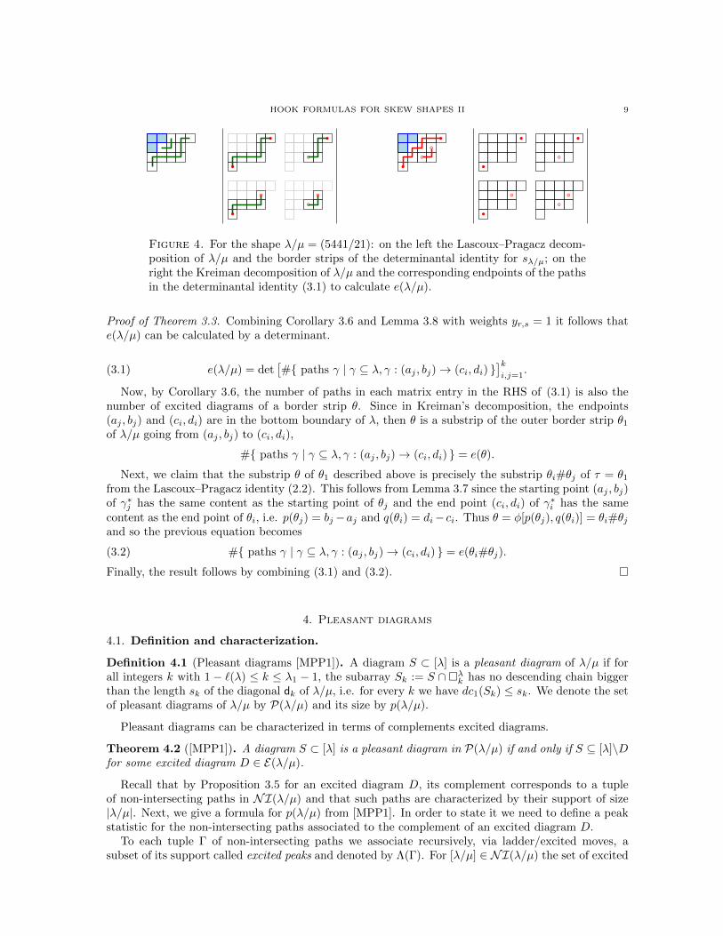
Figure 4. For the shape λ/µ = (5441/21): on the left the Lascoux–Pragacz decom-position of λ/µ and the border strips of the determinantal identity for sλ/µ; on theright the Kreiman decomposition of λ/µ and the corresponding endpoints of the pathsin the determinantal identity (3.1) to calculate e(λ/µ).
Proof of Theorem 3.3. Combining Corollary 3.6 and Lemma 3.8 with weights yr,s = 1 it follows thate(λ/µ) can be calculated by a determinant.
(3.1) e(λ/µ) = det[#{ paths γ | γ ⊆ λ, γ : (aj , bj)→ (ci, di) }
]ki,j=1
.
Now, by Corollary 3.6, the number of paths in each matrix entry in the RHS of (3.1) is also thenumber of excited diagrams of a border strip θ. Since in Kreiman’s decomposition, the endpoints(aj , bj) and (ci, di) are in the bottom boundary of λ, then θ is a substrip of the outer border strip θ1
of λ/µ going from (aj , bj) to (ci, di),
#{ paths γ | γ ⊆ λ, γ : (aj , bj)→ (ci, di) } = e(θ).
Next, we claim that the substrip θ of θ1 described above is precisely the substrip θi#θj of τ = θ1
from the Lascoux–Pragacz identity (2.2). This follows from Lemma 3.7 since the starting point (aj , bj)of γ∗j has the same content as the starting point of θj and the end point (ci, di) of γ∗i has the samecontent as the end point of θi, i.e. p(θj) = bj−aj and q(θi) = di− ci. Thus θ = φ[p(θj), q(θi)] = θi#θjand so the previous equation becomes
(3.2) #{ paths γ | γ ⊆ λ, γ : (aj , bj)→ (ci, di) } = e(θi#θj).
Finally, the result follows by combining (3.1) and (3.2). �
4. Pleasant diagrams
4.1. Definition and characterization.
Definition 4.1 (Pleasant diagrams [MPP1]). A diagram S ⊂ [λ] is a pleasant diagram of λ/µ if forall integers k with 1 − `(λ) ≤ k ≤ λ1 − 1, the subarray Sk := S ∩ �λk has no descending chain biggerthan the length sk of the diagonal dk of λ/µ, i.e. for every k we have dc1(Sk) ≤ sk. We denote the setof pleasant diagrams of λ/µ by P(λ/µ) and its size by p(λ/µ).
Pleasant diagrams can be characterized in terms of complements excited diagrams.
Theorem 4.2 ([MPP1]). A diagram S ⊂ [λ] is a pleasant diagram in P(λ/µ) if and only if S ⊆ [λ]\Dfor some excited diagram D ∈ E(λ/µ).
Recall that by Proposition 3.5 for an excited diagram D, its complement corresponds to a tupleof non-intersecting paths in NI(λ/µ) and that such paths are characterized by their support of size|λ/µ|. Next, we give a formula for p(λ/µ) from [MPP1]. In order to state it we need to define a peakstatistic for the non-intersecting paths associated to the complement of an excited diagram D.
To each tuple Γ of non-intersecting paths we associate recursively, via ladder/excited moves, asubset of its support called excited peaks and denoted by Λ(Γ). For [λ/µ] ∈ NI(λ/µ) the set of excited
10 ALEJANDRO MORALES, IGOR PAK, GRETA PANOVA
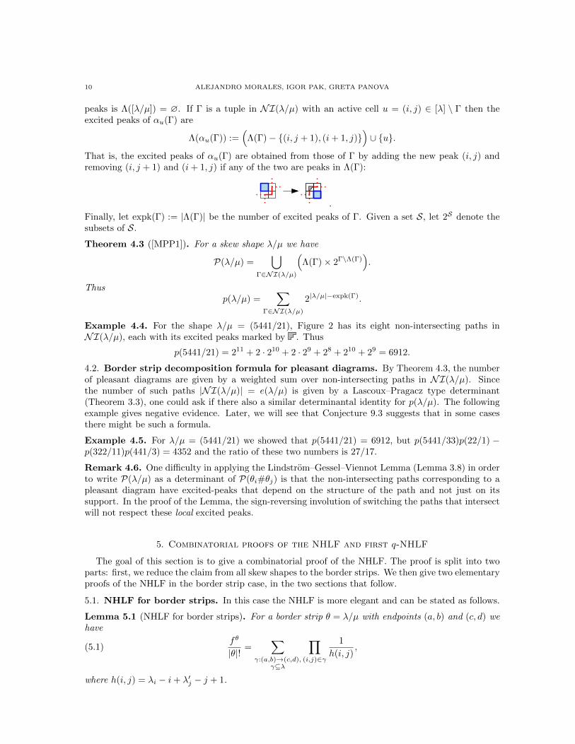
peaks is Λ([λ/µ]) = ∅. If Γ is a tuple in NI(λ/µ) with an active cell u = (i, j) ∈ [λ] \ Γ then theexcited peaks of αu(Γ) are
Λ(αu(Γ)) :=(
Λ(Γ)− {(i, j + 1), (i+ 1, j)})∪ {u}.
That is, the excited peaks of αu(Γ) are obtained from those of Γ by adding the new peak (i, j) andremoving (i, j + 1) and (i+ 1, j) if any of the two are peaks in Λ(Γ):
.
Finally, let expk(Γ) := |Λ(Γ)| be the number of excited peaks of Γ. Given a set S, let 2S denote thesubsets of S.
Theorem 4.3 ([MPP1]). For a skew shape λ/µ we have
P(λ/µ) =⋃
Γ∈NI(λ/µ)
(Λ(Γ)× 2Γ\Λ(Γ)
).
Thusp(λ/µ) =
∑Γ∈NI(λ/µ)
2|λ/µ|−expk(Γ).
Example 4.4. For the shape λ/µ = (5441/21), Figure 2 has its eight non-intersecting paths inNI(λ/µ), each with its excited peaks marked by . Thus
p(5441/21) = 211 + 2 · 210 + 2 · 29 + 28 + 210 + 29 = 6912.
4.2. Border strip decomposition formula for pleasant diagrams. By Theorem 4.3, the numberof pleasant diagrams are given by a weighted sum over non-intersecting paths in NI(λ/µ). Sincethe number of such paths |NI(λ/µ)| = e(λ/µ) is given by a Lascoux–Pragacz type determinant(Theorem 3.3), one could ask if there also a similar determinantal identity for p(λ/µ). The followingexample gives negative evidence. Later, we will see that Conjecture 9.3 suggests that in some casesthere might be such a formula.
Example 4.5. For λ/µ = (5441/21) we showed that p(5441/21) = 6912, but p(5441/33)p(22/1) −p(322/11)p(441/3) = 4352 and the ratio of these two numbers is 27/17.
Remark 4.6. One difficulty in applying the Lindstrom–Gessel–Viennot Lemma (Lemma 3.8) in orderto write P(λ/µ) as a determinant of P(θi#θj) is that the non-intersecting paths corresponding to apleasant diagram have excited-peaks that depend on the structure of the path and not just on itssupport. In the proof of the Lemma, the sign-reversing involution of switching the paths that intersectwill not respect these local excited peaks.
5. Combinatorial proofs of the NHLF and first q-NHLF
The goal of this section is to give a combinatorial proof of the NHLF. The proof is split into twoparts: first, we reduce the claim from all skew shapes to the border strips. We then give two elementaryproofs of the NHLF in the border strip case, in the two sections that follow.
5.1. NHLF for border strips. In this case the NHLF is more elegant and can be stated as follows.
Lemma 5.1 (NHLF for border strips). For a border strip θ = λ/µ with endpoints (a, b) and (c, d) wehave
(5.1)fθ
|θ|! =∑
γ:(a,b)→(c,d),γ⊆λ
∏(i,j)∈γ
1
h(i, j),
where h(i, j) = λi − i+ λ′j − j + 1.
HOOK FORMULAS FOR SKEW SHAPES II 11
Since the endpoints (a, b) and (c, d) are on the boundary of λ without loss of generality we assumethat (a, b) = (λ′1, 1) and (c, d) = (1, λ1). The proof is based on an identity of the following multivariatefunction. For a border strip λ/µ let
Fλ/µ(x | y) = Fλ/µ(x1, x2, . . . , xd | y1, y2 . . . , yn−d) :=∑
γ:(λ′1,1)→(1,λ1),γ⊆λ
∏(i,j)∈γ
1
xi − yj.
Note if we evaluate Fλ/µ(x | y) at xi = λi + d− i+ 1 and yj = d+ j − λ′j we obtain the RHS of (5.1),
(5.2) Fλ/µ(x | y)∣∣xi=λi+d−i+1,yj=d+j−λ′j
=∑
γ:(λ′1,1)→(1,λ1),γ⊆λ
∏(i,j)∈γ
1
h(i, j).
5.2. From border trips to all skew shapes. We need the analogue of Theorem 2.1 for fλ/µ.
Lemma 5.2 (Lascoux–Pragacz). If (θ1, . . . , θk) is a Lascoux–Pragacz decomposition of λ/µ, then
(5.3)fλ/µ
|λ/µ|! = det
[fθi#θj
|θi#θj |!
]ki,j=1
.
where f∅ = 1 and fφ[p,q] = 0 if φ[p, q] is undefined.
Proof. The result follows by doing the principal specialization in (2.2), using the theory of P -partitions[S4, Thm. 3.15.7] and letting q → 1. �
Proof of Theorem 1.2. Combining Theorem 5.1 and Lemma 5.2 we have
(5.4) fλ/µ = |λ/µ|! · det
∑γ:(aj ,bj)→(ci,di),
γ⊆λ
∏(r,s)∈γ
1
h(r, s)
k
i,j=1
.
Note that the weight 1/h(r, s) of each step in the path only depends on the coordinate (r, s) andthe fixed partition λ. By the weighted Lindstrom–Gessel–Viennot lemma (Lemma 3.8), with yr,s =1/h(r, s), we rewrite the RHS of (5.4) as a weighted sum over k-tuples non-intersecting paths Γ inNI(λ/µ). That is,
(5.5) fλ/µ = |λ/µ|! ·∑
(γ1,...,γk)∈NI(λ/µ)
∏(r,s)∈(γ1,...,γk)
1
h(r, s),
Finally, by Proposition 3.5 the supports of these non-intersecting paths are precisely the complementsof excited diagrams of λ/µ. This finished the proof of NHLF. �
5.3. Proof of the first q-NHLF. In this case too the SSYT q-analogue of NHLF is elegant and canbe stated as follows.
Lemma 5.3. For a border strip θ = λ/µ with end points (a, b) and (c, d) we have
(5.6) sθ(1, q, q2, . . . , ) =
∑γ:(aj ,bj)→(ci,di),
γ⊆λ
∏(i,j)∈γ
qλ′j−i
1− qh(i,j).
The proof is postponed to Section 7.4.
Lemma 5.4 (Lascoux–Pragacz).
(5.7) sλ/µ(1, q, q2, . . .) = det[sθi#θj (1, q, q
2, . . .)]ki,j=1
,
where s∅ = 1 and sφ[p,q] = 0 if θ[p, q] is undefined.
Proof. The result follows by doing a principal specialization in (2.2). �
12 ALEJANDRO MORALES, IGOR PAK, GRETA PANOVA
Proof of Theorem 1.3. Combining Lemma 5.4 and Lemma 5.3 we have
(5.8) sλ/µ(1, q, q2, . . .) = det
∑γ:(aj ,bj)→(ci,di),
γ⊆λ
∏(r,s)∈γ
qλ′s−r
1− qh(r,s)
k
i,j=1
.
Note that the weight of each step (r, s) in the path is qλ′s−r/(1 − qh(r,s)) which only depends on
the coordinate (r, s) and the fixed partition λ. By the weighted Lindstrom–Gessel–Viennot lemma
(Lemma 3.8), with yr,s = qλ′s−r/(1 − qh(r,s)), we rewrite the RHS of (5.8) as a weighted sum of
k-tuples non-intersecting paths in [λ]. That is,
(5.9) sλ/µ(1, q, q2, . . .) =∑
(γ1,...,γk)∈NI(λ/µ)
∏(r,s)∈(γ1,...,γk)
qλ′s−r
1− qh(r,s),
Finally, by Proposition 3.5 the supports of these non-intersecting paths are precisely the complementsof excited diagrams of λ/µ. Thus we obtain the (first q-NHLF). �
6. First proof of NHLF for border strips
In this section we give a proof of the NHLF for border strips based on a multivariate identity of theweighted sum of paths Fθ(x | y). We show that this weighted sum satisfies a recurrence from SYT.
6.1. Multivarite lemma. For any connected skew shape λ/µ, the entry 1 in a standard Youngtableau T of shape λ/µ will be in an inner corner of λ/µ. The remaining entries 2, 3, . . . , n form astandard Young tableau T ′ of shape λ/ν where µ → ν. Conversely, given a standard Young tableauT ′ of shape λ/ν where µ → ν, by filling the new cell with 0 we obtain a standard Young tableau ofshape λ/µ. Thus
(6.1) fλ/µ =∑µ→ν
fλ/ν .
We show combinatorially that for border strips λ/µ the multivariate rational function Fλ/µ(x | y)satisfies this type of relation.
Lemma 6.1 (Pieri–Chevalley formula for border strips).
(6.2) Fλ/µ(x | y) =1
(x1 − y1)
∑µ→ν
Fλ/ν(x | y).
Remark 6.2. A very similar multivariate relation holds for general skew shapes (the only difference isa different linear factor on the RHS of (6.2)), a fact proved by Ikeda and Naruse [IN] algebraically andcombinatorially by Konvalinka [Kon]. Our proof for border strips is different than these two proofs.See Section 10.2 for more details.
6.2. Proof of multivarite lemma. The rest of the section is devoted to the proof of Lemma 6.1.We start with some notation that will help us in the proof.
For cells A,B ∈ [λ] such that B is NW of A, let
F (A→ B) :=∑
γ:A→B,γ⊆[λ]
∏(i,j)∈γ
1
xi − yj,
so that Fλ/µ(x | y) = F ((λ′1, 1)→ (1, λ1)). For a given path γ let
H(γ) :=∏
(i,j)∈γ
1
(xi − yj)
HOOK FORMULAS FOR SKEW SHAPES II 13
be its multivariate weight. Let F (A∗, B) and F (A,B∗) denote similar rational functions where weomit the term xi − yj corresponding to A and B respectively. By abuse of notation F (A→ C∗ → B)
denotes the product F (A → C∗)F (C∗ → B). Let C and C denote the boxes in the Young diagram[λ] that are right above and right below C, respectively. Let Rk(λ) denote the kth row of the Youngdiagram of λ.
We will show by induction on the total length of the path between A and B that
(6.3) F (A→ B) =1
x1 − y1
∑C
F (A→ C∗ → B),
where the sum is over inner corners C of λ/µ. This relation implies the desired result.For the base case λ = (2, 2) and µ = (1), the shape (2, 2)/(1) has inner corners (1, 2) and (2, 1). We
have
F ((2, 1)→ (1, 2)) =1
(x2 − y1)(x2 − y2)(x1 − y2)+
1
(x2 − y1)(x1 − y1)(x1 − y2)
=x1 − y1 + x2 − y2
(x1 − y1)(x2 − y1)(x1 − y2)(x2 − y2)
=1
x1 − y1
(1
(x2 − y1)(x2 − y2)+
1
(x2 − y2)(x1 − y2)
),
which equals [F ((1, 2)→ (2, 1)∗) + F ((1, 2)∗ → (2, 1))] /(x1 − y1), thus proving the relation.The next sublemma will be useful in the inductive step later.
Lemma 6.3. For cells A = (d, r) and B = (1, s) in [λ] with r ≤ s, we have
(x1 − xd)F (A→ B) =∑C
F (A→ C∗ → B),
where the sum is over inner corners C of λ/µ.
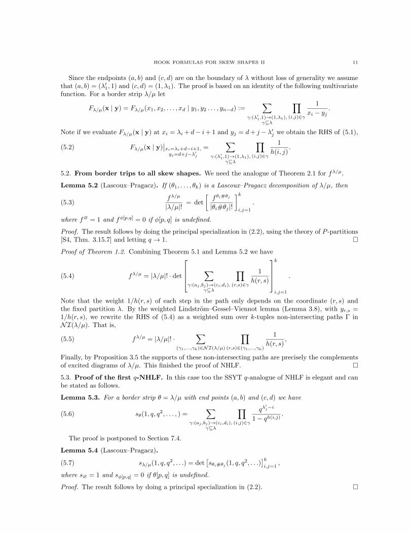
Proof. We can write xk − xk−1 = (xk − yj)− (xk−1− yj) for any j. Let γ be a path from A to B, andsuppose that it crosses from row k to row k − 1 in column j for some j. Then both points (k, j) ∈ γand (k − 1, j) ∈ γ
(6.4) (xk − xk−1)H(γ) = (xk − yj)H(γ)− (xk−1 − yj)H(γ) = H(γ \ (k, j))−H(γ \ (k − 1, j)).
Since every path from A to B crosses from row k to row k− 1 at some cell, denoted by C = (k, j), by(6.4) we have the following:
(xk − xk−1)F (A→ B) =∑
C∈Rk(λ)
(F (A→ C∗)F (C → B)− F (A→ C)F (C
∗ → B))
=∑
C∈Rk(λ)
F (A→ C∗ → C → B)−∑
C1∈Rk−1(λ)
F (A→ C1 → C∗1 → B) = ∗©
where in the last line we denote C1 = C – a box in row k − 1, and we note that the existence of theboxes below and above is implicit in the specified path functions F .
Let us now rewrite the RHS. in the last equation in a different way. Note that the paths A →C∗ → C → B can be thought as paths from A to B without their outer corner on row k, and, likewise,the paths A → C1 → C∗1 → B are paths A → B without the inner corner on row k − 1. However,they can both be thought as composed of two paths, A → A1 and B1 → B, where A1 is the lastbox on row k (or row k + 1 if C was the only cell on row k), B1 is the first box on row k − 1 (orthe box above C, in row k − 2) and A1’s top right vertex is the same as B1’s bottom left (i.e. theboxes have that common vertex), or as in the second case B1 is one box above A1. In the case ofA → C∗ → C → B = A → A1, B1 → B, we must have that A1 is not the last box in the row (for C
14 ALEJANDRO MORALES, IGOR PAK, GRETA PANOVA
to exist), and for A→ C1 → C∗1 → B = A→ A1, B1 → B there are no restrictions. Thus
(xk − xk−1)F (A→ B) = ∗©=
∑A1 6=(k,λk),B1
F (A→ A1)F (B1 → B) −∑A1,B1
F (A→ A1)F (B1 → B)
=∑
j:A1=(k+1,j),B1=(k−1,j)
F (A→ A1)F (B1 → B)−,∑
j:A1=(k,j),B1=(k−2,j)
(F (A→ A1)F (B1 → B)− F (A→ D∗k → B)
),
where all terms cancel except for the cases where A1, C,B1 are in the same column, and when C is anouter corner of λ on row k, denoted by Dk (if such corner exists).
Finally, since xd − x1 =∑k(xk − xk−1), we have
(xd − x1)F (A→ B) =∑k
(xk − xk−1)F (A→ B)
=∑
k,j:A1=(k+1,j),B1=(k−1,j)
F (A→ A1)F (B1 → B) −∑
k,j:A1=(k,j),B1=(k−2,j)
(F (A→ A1)F (B1 → B)− F (A→ D∗k → B)
)
= −∑k
F (A→ D∗k → B),
since all other terms cancel across the various values for k, and we obtain the desired identity. �
We continue with the proof of Lemma 6.1. In a path γ : A→ B the first step from A is either rightto cell Ar or up to cell Au. Note that in the first case A is then an inner corner of λ/µ. Thus
F (A→ B) =1
xd − y1(F (Ar → B) + F (Au → B)) .
By induction the term F (Au → B) becomes
(6.5) F (A→ B) =1
xd − y1
(F (Ar → B) +
1
x1 − y1
∑C
F (Au → C∗ → B)
).
On the other hand, since a step to Ar indicates that A is an inner corner then the RHS of (6.3)equals
1
x1 − y1
∑C
F (A→ C∗ → B) =1
x1 − y1
[F (Ar → B) +
1
xd − y1
∑C
F (A∗ → C∗ → B)
].
Again, depending on the first step of the paths we split F (A∗ → C∗ → B) into F (Ar → C∗ → B) andF (Au → C∗ → B) so the above equation becomes
(6.6)1
x1 − y1
∑C
F (A→ C∗ → B)
=1
x1 − y1
[F (Ar → B) +
1
xd − y1
∑C
(F (Ar → C∗ → B) + F (Au → C∗ → B)
)].
Finally, by (6.5) and (6.6) if we subtract the LHS and RHS of (6.3) the terms with Au → C∗ → Bcancel. Collecting the terms with Ar → B we obtain
(6.7) F (A→ B) − 1
x1 − y1
∑C
F (A→ C∗ → B)
=x1 − xd
(x1 − y1)(xd − y1)F (Ar → B) − 1
(x1 − y1)(xd − y1)
∑C
F (Ar → C∗ → B1) .
HOOK FORMULAS FOR SKEW SHAPES II 15
Lastly, the RHS above is zero since by Lemma 6.3 we have
(x1 − xd)F (Ar → B) =∑C
F (Ar → C∗ → B).
Thus the desired relation (6.3) follows.
6.3. Proof of NHLF for border strips. In this section we use Lemma 6.1 to prove Theorem 5.1.Let Hλ/µ denote the RHS of (5.2). We prove by induction on n = |λ/µ| that fλ/µ = n! ·Hλ/µ.We start with (6.2) and evaluate xi = λi + d− i+ 1 and yj = d+ j − λ′j , by (5.2) we obtain
n ·Hλ/µ =∑µ→ν
Hλ/ν .
Multiplying both sides by (n− 1)! and using induction we obtain
n! ·Hλ/µ =∑µ→ν
fλ/ν .
By (6.1) the result follows.
7. Second proof of NHLF for border strips
In this section we give another proof of the NHLF for border strips based on another multivariateidentity involving factorial Schur functions. The proof consists of two steps. First we show that a ratioof an evaluation of factorial Schur functions equals the weighted sum of paths Fθ(x | y). Second weshow how the ratio of factorial Schur functions properly specialized equals fλ/µ and sλ/µ(1, q, q2, . . .).
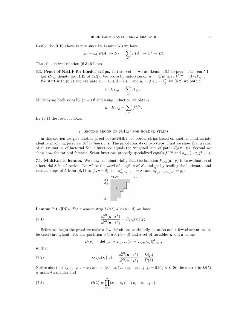
7.1. Multivarite lemma. We show combinatorially that the function Fλ/µ(x | y) is an evaluation of
a factorial Schur function. Let zλ be the word of length n of x’s and y’s by reading the horizontal andvertical steps of λ from (d, 1) to (1, n− d): i.e. zλλi+d−i+1 = xi and zλλ′j+n−d−j+1 = yj :
x1x2
xd
y1y2 yn−d
λ
.
Lemma 7.1 ([IN]). For a border strip λ/µ ⊆ d× (n− d) we have
(7.1)s
(d)µ (x | zλ)
s(d)λ (x | zλ)
= Fλ/µ(x | y).
Before we begin the proof we make a few definitions to simplify notation and a few observations tobe used throughout. For any partition ν ⊆ d× (n− d) and a set of variables x and z define
D(ν) := det[(xi − z1) . . . (xi − zνj+d−j)]di,j=1,
so that
(7.2) Gλ/µ(x | y) :=s
(d)µ (x | zλ)
s(d)λ (x | zλ)
=D(µ)
D(λ).
Notice also that zλj+1+d−j = xj and so (xi− z1) . . . (xi− zλj+d−j) = 0 if j < i. So the matrix in D(λ)is upper-triangular and
(7.3) D(λ) =
d∏i=1
(xi − z1) · · · (xi − zλi+d−i).
16 ALEJANDRO MORALES, IGOR PAK, GRETA PANOVA
7.2. Proof of multivariate lemma. To prove Lemma 7.1 we verify that both sides of (7.1) satisfythe following trivial path identity. The first step of a path γ : (λ′1, 1)→ (1, λ1) is either (0, 1) (up) or(1, 0) (right) provided λd > 1. So
(7.4) (xd − y1)Fλ/µ(x | y) = Fλ−λd/µ−µd−1(x1, . . . , xd−1 | y) + Fλ−1/µ−1(x | y2, . . . , yn−d),
where the second term on the RHS vanishes if λd = 1.
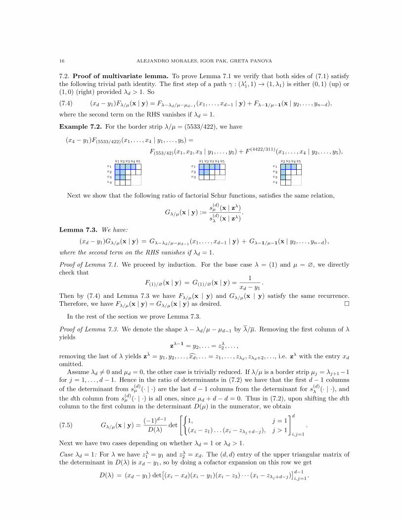
Example 7.2. For the border strip λ/µ = (5533/422), we have
(x4 − y1)F(5533/422)(x1, . . . , x4 | y1, . . . , y5) =
F(553/42)(x1, x2, x3 | y1, . . . , y5) + F (4422/311)(x1, . . . , x4 | y2, . . . , y5),y1y2y3y4y5
x1
x2
x3
x4
x1
x2
x3
x4
y2y3y4y5
x1
x2
x3
y1y2y3y4y5
Next we show that the following ratio of factorial Schur functions, satisfies the same relation,
Gλ/µ(x | y) :=s
(d)µ (x | zλ)
s(d)λ (x | zλ)
.
Lemma 7.3. We have:
(xd − y1)Gλ/µ(x | y) = Gλ−λd/µ−µd−1(x1, . . . , xd−1 | y) + Gλ−1/µ−1(x | y2, . . . , yn−d) ,
where the second term on the RHS vanishes if λd = 1.
Proof of Lemma 7.1. We proceed by induction. For the base case λ = (1) and µ = ∅, we directlycheck that
F(1)/∅(x | y) = G(1)/∅(x | y) =1
xd − y1.
Then by (7.4) and Lemma 7.3 we have Fλ/µ(x | y) and Gλ/µ(x | y) satisfy the same recurrence.Therefore, we have Fλ/µ(x | y) = Gλ/µ(x | y) as desired. �
In the rest of the section we prove Lemma 7.3.
Proof of Lemma 7.3. We denote the shape λ− λd/µ− µd−1 by λ/µ. Removing the first column of λyields
zλ−1 = y2, . . . = zλ2 , . . . ,
removing the last of λ yields zλ = y1, y2, . . . , xd, . . . = z1, . . . , zλd , zλd+2, . . ., i.e. zλ with the entry xdomitted.
Assume λd 6= 0 and µd = 0, the other case is trivially reduced. If λ/µ is a border strip µj = λj+1−1for j = 1, . . . , d − 1. Hence in the ratio of determinants in (7.2) we have that the first d − 1 columns
of the determinant from s(d)µ (· | ·) are the last d − 1 columns from the determinant for s
(d)λ (· | ·), and
the dth column from s(d)µ (· | ·) is all ones, since µd + d − d = 0. Thus in (7.2), upon shifting the dth
column to the first column in the determinant D(µ) in the numerator, we obtain
(7.5) Gλ/µ(x | y) =(−1)d−1
D(λ)det
[{1, j = 1
(xi − z1) . . . (xi − zλj+d−j), j > 1
]di,j=1
.
Next we have two cases depending on whether λd = 1 or λd > 1.
Case λd = 1: For λ we have zλ1 = y1 and zλ2 = xd. The (d, d) entry of the upper triangular matrix ofthe determinant in D(λ) is xd − y1, so by doing a cofactor expansion on this row we get
D(λ) = (xd − y1) det[(xi − xd)(xi − y1)(xi − z3) · · · (xi − zλj+d−j)
]d−1
i,j=1.
HOOK FORMULAS FOR SKEW SHAPES II 17
By factoring xi − z2 = xi − xd from each row above we get
D(λ) = (xd − y1) det[(xi − y1)(xi − z3) · · · (xi − zλj+d−j)
]d−1
i,j=1
d−1∏i=1
(xi − xd) .
Since zλ1 = y1 and zλj = zλj+1 for j = 2, . . . , d− 1, then by relabelling we get
(7.6) D(λ) = (xd − y1)D(λ)
d−1∏i=1
(xi − xd) .
For µ we have µd = µd−1 = 0 so the matrix in D(µ) has a dth column of ones
D(µ) = det
. . . (x1 − z1) · · · (x1 − zµj+d−j) · · · (x1 − y1) 1. . . (x2 − z1) · · · (x2 − zµj+d−j) · · · (x2 − y1) 1...
...0 · · · 0 (xd − y1) 1
Then, by adding (xd − y1) to each entry in the (d− 1)th column, the determinant remains unchangedbut the last row becomes 0 . . . 01,
D(µ) = det
1, j = d
xi − xd, j = d− 1
(xi − z1) . . . (xi − zµj+d−j), j < d− 1
d
i,j=1
Next, we do a cofactor expansion on the last row and then we factor xi − z2 = xi − xd from each row,
D(µ) = det
[{xi − xd, j = d− 1
(xi − z1)(xi − z2) . . . (xi − zµj+d−j), j < d− 1
]d−1
i,j=1
= det
[{1, j = d− 1
(xi − z1) (xi − xd) . . . (xi − zµj+d−j), j < d− 1
]d−1
i,j=1
d−1∏i=1
(xi − xd).
Again, since zλ1 = y1 and zλj = zλj+1 for j = 2, . . . , d− 1, we have by relabeling
(7.7) D(µ) = D(µ)
d−1∏i=1
(xi − xd).
We now combine (7.6) and (7.7) in (xd − y1)Gλ/µ(· | ·),
(xd − y1)Gλ/µ(x | y) = (xd − y1)D(µ)
∏d−1i=1 (xi − xd)
(xd − y1)D(λ)∏d−1i=1 (xi − xd)
= Gλ/µ(x1, . . . , xd−1 | y),
confirming the desired identity in this case as well since the term for λ− 1/µ− 1 is vacuously zero.
Case λd > 1: Using z1 = y1 we have
Gλ−1/µ−1(x | y2, . . . , yn−d) =(−1)d−1
D(λ− 1)det
[{1, j = 1
(xi − z2) . . . (xi − zλj+d−j), j > 1
]di,j=1
=(−1)d−1
D(λ)det
[{1, j = 1
(xi − z2) . . . (xi − zλj+d−j), j > 1
]di,j=1
·d∏i=1
(xi − y1)
=(−1)d−1
D(λ)det
[{(xi − y1), j = 1
(xi − z1) . . . (xi − zλj+d−j), j > 1
]di,j=1
18 ALEJANDRO MORALES, IGOR PAK, GRETA PANOVA
Similarly, we have:
(7.8) Gλ/µ(x1, . . . , xd−1 | y)
=(−1)d−2
D(λ)det
[{(xi − xd), j = 1
(xi − z1) . . . (xi − zλj−1+d−j−1), 2 ≤ j ≤ d− 1
]d−1
i,j=1
·λd∏j=1
(xd − yj)
Next, we add the two determinants in (7.5) and (7.8) using the multilinearity property on the firstcolumn to obtain
(xd − y1)Gλ/µ(x | y)−Gλ−1/µ−1(x | y2, . . . , yn−d) =(−1)d−1
D(λ)×det
[{(xd − y1), j = 1
(xi − z1) . . . (xi − zλj+d−j), j > 1
]di,j=1
− det
[{(xi − y1), j = 1
(xi − z1) . . . (xi − zλj+d−j), j > 1
]di,j=1
=
(−1)d−1
D(λ)det
[{xd − xi, j = 1
(xi − z1) . . . (xi − zλj+d−j), j > 1
]di,j=1
=: (∗)
Consider the row i = d in the last determinant. The entries there are all 0, except when j = d:when j = 1 we have xd − xi = 0 for i = d, when j ∈ [2, d− 1] we have λj + d− j ≥ λd + 1, and since
zλd+1 = xd we have∏λj+d−jr=1 (xd− zr) = 0. Using the cofactor expansion we compute the determinant
in the last equation as the principal minor of the matrix times the (d, d) entry:
(∗) =(−1)d−1
D(λ)det
[{xd − xi, j = 1
(xi − z1) . . . (xi − zλj+d−j), j > 1
]d−1
i,j=1
(xd − z1) · · · (xd − zλd).
We now compare this with equation (7.8), realizing that z1, . . . , zλd = y1, . . . , yλd , so the lastexpression coincides with Gλ/µ(x | y) as desired. Notice also that if j < i, we have λj + d − j ≥λi + d− i+ 1, and since xi = zλi+d−i+1, the terms above are 0 when j < i and j 6= 1. �
7.3. Proof of NHLF for border strips.
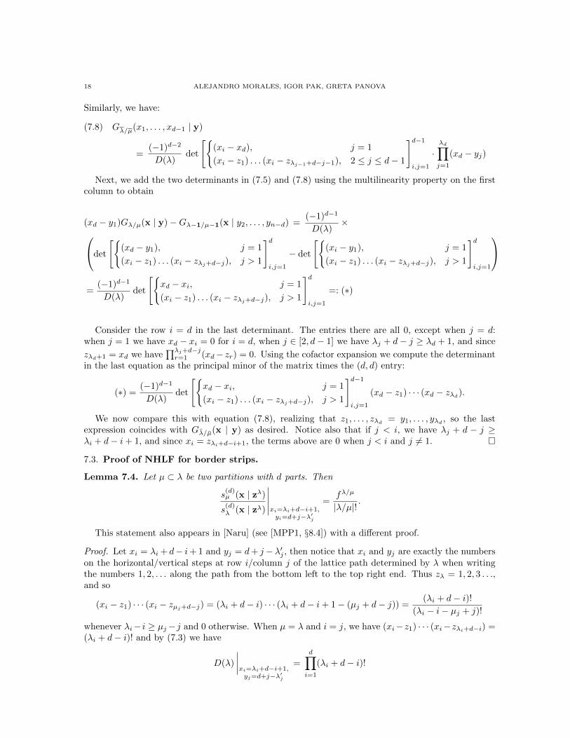
Lemma 7.4. Let µ ⊂ λ be two partitions with d parts. Then
s(d)µ (x | zλ)
s(d)λ (x | zλ)
∣∣∣∣∣xi=λi+d−i+1,yi=d+j−λ′j
=fλ/µ
|λ/µ|! .
This statement also appears in [Naru] (see [MPP1, §8.4]) with a different proof.
Proof. Let xi = λi + d− i+ 1 and yj = d+ j − λ′j , then notice that xi and yj are exactly the numberson the horizontal/vertical steps at row i/column j of the lattice path determined by λ when writingthe numbers 1, 2, . . . along the path from the bottom left to the top right end. Thus zλ = 1, 2, 3 . . .,and so
(xi − z1) · · · (xi − zµj+d−j) = (λi + d− i) · · · (λi + d− i+ 1− (µj + d− j)) =(λi + d− i)!
(λi − i− µj + j)!
whenever λi− i ≥ µj−j and 0 otherwise. When µ = λ and i = j, we have (xi−z1) · · · (xi−zλi+d−i) =(λi + d− i)! and by (7.3) we have
D(λ)
∣∣∣∣xi=λi+d−i+1,yj=d+j−λ′j
=
d∏i=1
(λi + d− i)!

HOOK FORMULAS FOR SKEW SHAPES II 19
Then, by definition and (7.2), we have
Gλ/µ(x | y)
∣∣∣∣∣xi=λi+d−i+1,yj=d+j−λ′j
=D(µ)
D(λ)
∣∣∣∣∣xi=λi+d−i+1,yj=d+j−λ′j
=det[(λi + d− i)!/(λi − i− µj + j)!
]di,j=1∏d
i=1(λi + d− i)!
= det
[1
(λi − i− µj + j)!
]di,j=1
Multiplying the last determinant by |λ/µ|!, we recognize the exponential specialization of the Jacobi-Trudi identity for the ordinary sλ/µ giving fλ/µ (a formula due to Aitken, see e.g. [S4, Cor. 7.16.3]).Hence we get the desired formula. �
Second proof of Theorem 5.1. We start with the relation from Lemma 7.1 and evaluate xi = λi+d−i+1and yj = d+ j − λ′j . In the RHS by (5.2) we immediately obtain the RHS of (5.1).
Next, we do the same evaluation on the ratio of factorial Schur functions applying Lemma 7.4 thatgives the ratio of factorial Schurs as fλ/µ/|λ/µ|!. �
7.4. SSYT q-analogue for border strips. To wrap up the section we show how the tools developedto prove Theorem 5.1 also yield the SSYT q-analogue for border strips.
Corollary 7.5 ((first q-NHLF) for border strips). For a border strip θ = λ/µ with end points (a, b)and (c, d) we have
(7.9) sθ(1, q, q2, . . . , ) =
∑γ:(aj ,bj)→(ci,di),
γ⊆λ
∏(i,j)∈γ
qλ′j−i
1− qh(i,j).
Proof. We start with (7.1) from Lemma 7.1 and evaluate both sides at xi = qλi+d−i+1 and yj =
qd+j−λ′j . The path series Fλ/µ(x | y) gives the RHS of (7.9)
Fλ/µ(x | y)∣∣xi=q
λi+d−i+1,
yj=qd+j−λ′j
=∑
γ:(aj ,bj)→(ci,di),γ⊆λ
∏(i,j)∈γ
qλ′j−i
1− qh(i,j).
Next, by [MPP1, §4] the evaluation of the ratio of the factorial Schur functions gives the principalspecialization of the Schur function, the LHS of (7.9)
s(d)µ (x | zλ)
s(d)λ (x | zλ)
∣∣∣∣∣xi=qλi+d−i+1,
yj=qd+j−λ′j
= sθ(1, q, q2, . . . ).
�
7.5. Lascoux–Pragacz identity for factorial Schur functions. Lemma 7.1 holds for connectedskew shape λ/µ in terms of non-intersecting paths Γ = (γ1, . . . , γk) in NI(λ/µ) (i.e. complements ofexcited diagrams).
Fλ/µ(x | y) :=∑
Γ∈NI(λ/µ)
∏(r,s)∈Γ
1
xr − ys=
∑D∈E(λ/µ)
∏(r,s)∈[λ]\D
1
xr − ys.
Ikeda and Naruse [IN] showed algebraically the following identity that we call the multivariate NHLF.
Theorem 7.6 ([IN]). For a connected skew shape λ/µ ⊆ d× (n− d) we have
(7.10)s
(d)µ (x | zλ)
s(d)λ (x | zλ)
= Fλ/µ(x | y).
20 ALEJANDRO MORALES, IGOR PAK, GRETA PANOVA
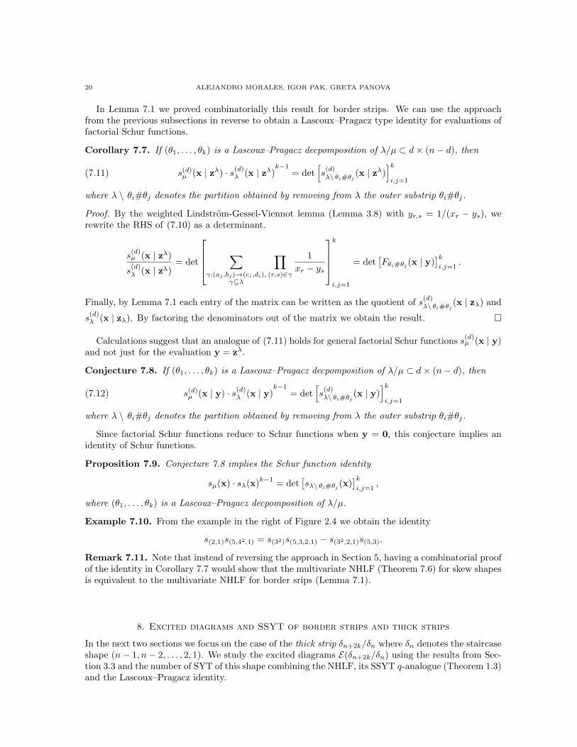
In Lemma 7.1 we proved combinatorially this result for border strips. We can use the approachfrom the previous subsections in reverse to obtain a Lascoux–Pragacz type identity for evaluations offactorial Schur functions.
Corollary 7.7. If (θ1, . . . , θk) is a Lascoux–Pragacz decpomposition of λ/µ ⊂ d× (n− d), then
(7.11) s(d)µ (x | zλ) · s(d)
λ (x | zλ)k−1
= det[s
(d)λ\ θi#θj (x | z
λ)]ki,j=1
where λ \ θi#θj denotes the partition obtained by removing from λ the outer substrip θi#θj.
Proof. By the weighted Lindstrom-Gessel-Viennot lemma (Lemma 3.8) with yr,s = 1/(xr − ys), werewrite the RHS of (7.10) as a determinant.
s(d)µ (x | zλ)
s(d)λ (x | zλ)
= det
∑γ:(aj ,bj)→(ci,di),
γ⊆λ
∏(r,s)∈γ
1
xr − ys
k
i,j=1
= det[Fθi#θj (x | y)
]ki,j=1
.
Finally, by Lemma 7.1 each entry of the matrix can be written as the quotient of s(d)λ\ θi#θj (x | zλ) and
s(d)λ (x | zλ). By factoring the denominators out of the matrix we obtain the result. �
Calculations suggest that an analogue of (7.11) holds for general factorial Schur functions s(d)µ (x | y)
and not just for the evaluation y = zλ.
Conjecture 7.8. If (θ1, . . . , θk) is a Lascoux–Pragacz decpomposition of λ/µ ⊂ d× (n− d), then
(7.12) s(d)µ (x | y) · s(d)
λ (x | y)k−1
= det[s
(d)λ\ θi#θj (x | y)
]ki,j=1
where λ \ θi#θj denotes the partition obtained by removing from λ the outer substrip θi#θj.
Since factorial Schur functions reduce to Schur functions when y = 0, this conjecture implies anidentity of Schur functions.
Proposition 7.9. Conjecture 7.8 implies the Schur function identity
sµ(x) · sλ(x)k−1
= det[sλ\ θi#θj (x)
]ki,j=1
,
where (θ1, . . . , θk) is a Lascoux–Pragacz decpomposition of λ/µ.
Example 7.10. From the example in the right of Figure 2.4 we obtain the identity
s(2,1)s(5,42,1) = s(32)s(5,3,2,1) − s(32,2,1)s(5,3).
Remark 7.11. Note that instead of reversing the approach in Section 5, having a combinatorial proofof the identity in Corollary 7.7 would show that the multivariate NHLF (Theorem 7.6) for skew shapesis equivalent to the multivariate NHLF for border srips (Lemma 7.1).
8. Excited diagrams and SSYT of border strips and thick strips
In the next two sections we focus on the case of the thick strip δn+2k/δn where δn denotes the staircaseshape (n− 1, n− 2, . . . , 2, 1). We study the excited diagrams E(δn+2k/δn) using the results from Sec-tion 3.3 and the number of SYT of this shape combining the NHLF, its SSYT q-analogue (Theorem 1.3)and the Lascoux–Pragacz identity.

HOOK FORMULAS FOR SKEW SHAPES II 21
8.1. Excited diagrams and Catalan numbers. We start enumerating the excited diagrams of theshape δn+2k/δn.
Corollary 8.1. We have: e(δn+2/δn) = Cn, e(δn+4/δn) = CnCn+2 − C2n+1,
(8.1) e(δn+2k/δn) = det[Cn−2+i+j ]ki,j=1 =
∏1≤i<j≤n
2k + i+ j − 1
i+ j − 1.
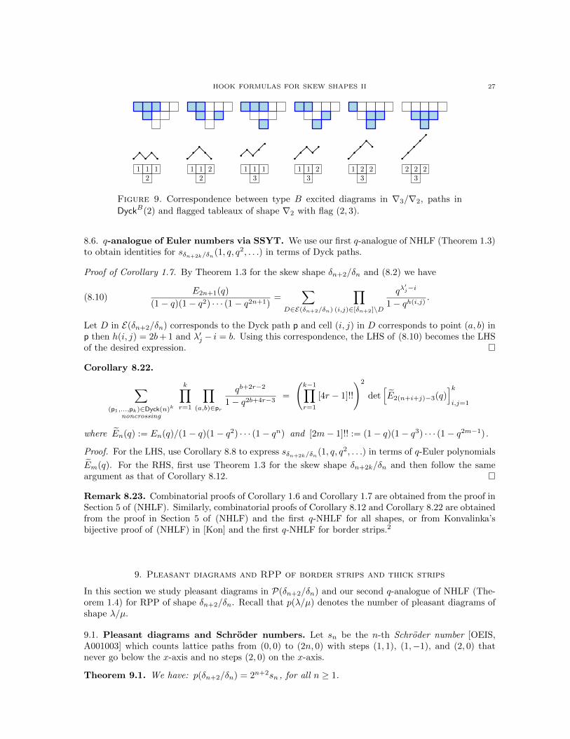
Proof. We start with the case k = 1 for the zigzag border strip δn+2/δn. By Proposition 3.5 thecomplement of excited diagrams of δn+2/δn are paths γ : (n+1, 1)→ (1, n+1), γ ⊆ δn+2. By rotatingthese paths 45◦ clockwise one obtain the Dyck paths in Dyck(n) as illustrated in Figure 5. Thuse(δn+2/δn) = Cn.
For general k, the shape δn+2k/δn has a Lascoux–Pragacz decomposition into k maximal borderstrips (θ1, . . . , θk) where θi is the zigzag strip from (n + 2k − 2i − 1, 1) to (1, n + 2k − 2i − 1) (seeFigure 6: Left). Then by Theorem 3.3 we have
e(δn+2k/δn) = det[e(θi#θj)
]ki,j=1
.
The cutting strip τ of the decomposition of δn+2k/δn is the zigzag θ1. The strips θi#θj in thedeterminant, being substrips of θ1, are themselves zigzags. The strip θi#θj in θ1 consists of the cellswith content from 2 + 2j − n− 2k to n+ 2k − 2i− 2. So the strip is a zigzag δm+2/δm of size 2m+ 1where m = n+ 2k+ i+ j+ 2. Since we already know shapes δm+2/δm have Cm excited diagrams thenthe above determinant becomes
e(δn+2k/δn) = det[Cn+2k−i−j−2
]ki,j=1
= det[Cn+i+j−2
]ki,j=1
,
where the last equality is obtained by relabelling the matrix. This proves the first equality.To prove the second equality we use the characterization of excited diagrams as flagged tableaux.
By [MPP1, Prop. 3.6], excited diagrams in E(δn+2k/δn) are in bijection with flagged tableaux of shapeδn with flag (k + 1, k + 2, . . . , k + n − 1). By subtracting i to all entries in row i, these tableaux areequivalent to reverse plane partitions of shape δn with entries ≤ k which are counted by the givenproduct formula due to Proctor (unpublished research announcement 1984; see [FK]). �
Remark 8.2. Note that by [MPP1, Prop. 3.6], excited diagrams in E(δn+2k+1/δn) are in correspon-dence with flagged tableaux of shape δn with flag (k + 1, k + 2, . . . , k + n − 1), thus |E(δn+2k/δn)| =|E(δn+2k+1/δn)|. In what follows the formulas for the even case δn+2k are simpler than those of theodd case so we omit the latter.
1 12
1 13
1 22
1 23
2 23
Figure 5. Correspondence between excited diagrams in δ5/δ3, Dyck paths in Dyck(3)and flagged tableaux of shape δ3 with flag (2, 3).
From the first determinantal formula for e(λ/µ) (Proposition 3.1) we easily obtain the followingcurious determinantal identity (see also §10.4).
Corollary 8.3. We have:
det
[(n− i+ j
i
)]n−1
i,j=1
= Cn .

22 ALEJANDRO MORALES, IGOR PAK, GRETA PANOVA
Proof. By Corollary 8.1, we have |E(δn+2/δn)| = Cn. We apply Proposition 3.1 to the shape δn+2/δn,where the vector fδn+2/δn = (2, 3, . . . , n), see §3.2. This expresses |E(δn+2/δn)| as the given determi-nant, and the identity follows. �
Next we give a description of the excited diagrams of the shape δn+2k/δn. Let FanDyck(k, n) bethe set of tuples (p1, . . . , pk) of k noncrossing Dyck paths from (0, 0) to (2n, 0) (see Figure 6: Right).We call such tuples k-fans of Dyck paths. It is known [SV] that fans of Dyck pahts are counted by thedeterminant of Catalan numbers and the product formula in (8.1).
Corollary 8.4. We have e(δn+2k/δn) = |FanDyck(k, n)| and the complements of the excited diagramscorrespond to k-fans of paths in FanDyck(k, n).
Proof. By Proposition 3.5 the complements of excited diagrams in E(δn+2k/δn) correspond to k-tuplesof nonintersecting paths in NI(δn+2k/δn) (paths obtained via ladder moves from the original paths(γ∗1 , . . . , γ
∗k) of the Kreiman outer decomposition of δn+2k/δn).
The path γ∗i consists of zigzag path p∗i of 2n+1 cells bookended by a vertical and horizontal segmentof k − i cells each (see Figure 6:Middle). Because the excited/ladder moves preserve the contents ofthe cells of δn, the path γi in (γ1, . . . , γk) ∈ NI(δn+2k/δn) will consist of a Dyck path pi bookendedby the same vertical and horizontal segments as in γ∗i . Thus the map (γ1, . . . , γk) 7→ (p1, . . . , pk)denoted by ϕ is a correspondence between NI(δn+2k/δn) and FanDyck(k, n). See Figure 6, right, foran example. �
Remark 8.5. Fans of Dyck paths in FanDyck(k, n) are equinumerous with k-triangulations of an(n+ 2k)-gon [Jon] (see also [S5, A12] and [SS] for a bijection for general k).
θ1θ2θ3γ∗1
γ∗2
γ∗3 7→
ϕ
Figure 6. Left, Middle: the Lascoux–Pragacz and the Kreiman outer decompositionsof the shape δ3+6/δ3. Right: the hook-lengths of an excited diagram of δ3+6/δ3corresponding to the 3-fan of Dyck paths on the right. Each gray area has cells withproduct of hook-lengths (3!! · 7!!).
8.2. Determinantal identity of Schur functions of thick strips. Observe that SYT of shapeδn+2/δn are in bijection with alternating permutations of size 2n+ 1. These permutations are countedby the odd Euler number E2n+1. Thus,
fδn+2/δn = E2n+1 .
Let En(q) be as in the introduction, the q-analogue of Euler numbers.1
Example 8.6. We have: E1(q) = E2(q) = 1, E3(q) = q2 + q, E4(q) = q4 + q3 + 2q2 + q, andE5(q) = q8 + 2q7 + 3q6 + 4q5 + 3q4 + 2q3 + q2 .
1In the survey [S3, §2], our En(q) is denoted by E?n(q).

HOOK FORMULAS FOR SKEW SHAPES II 23
By the theory of (P, ω)-partitions, we have:
(8.2) E2n+1(q) = sδn+2/δn(1, q, q2, . . .) ·2n+1∏i=1
(1− qi) .
Next we apply the Lascoux–Pragacz identity to the shape δn+2k/δn.
Corollary 8.7 (Lascoux–Pragacz for δn+2k/δn). We have:
sδn+2k/δn(x) = det[sδn+i+j/δn−2+i+j
(x)]ki,j=1
.
Proof. By Theorem 2.1 for the shape δn+2k/δn we have
sδn+2k/δn(x) = det[sθi#θj (x)
]ki,j=1
,
where (θ1, . . . , θk) is the decomposition of the shape δn+2k/δn into k maximal border strips. As in theproof of Corollary 8.1, the strip θi#θj has shape δm+2/δm for m = n + 2k − i − j + 2. Thus, afterrelabelling the matrix, the above equation becomes the desired expression. �
Corollary 8.8. We have:
sδn+2k/δn(1, q, q2, . . .) = det[E2(n+i+j)−3(q)
]ki,j=1
,
where
En(q) :=En(q)
(1− q)(1− q2) · · · (1− qn).
Proof. The result follows from Corollary 8.7 and equation (8.2). �
Taking the limit q → 1 in Corollary 8.8 we get corresponding identities for fδn+2k/δn .
Corollary 8.9. We have:
fδn+2k/δn
|δn+2k/δn|!= det
[E2(n+i+j)−3
]ki,j=1
, where En :=Enn!
.
Remark 8.10. Baryshnikov and Romik [BR] gave similar determinantal formulas for the number ofstandard Young tableaux of skew shape (n+m− 1, n+m− 2, . . . ,m)/(n− 1, n− 2, . . . , 1), extendingthe method of Elkies (see e.g. [AR, Ch. 14]).
In a different direction, one can use Corollary 8.9 when n = 1, 2 to obtain the following determinantformulas for Euler numbers in terms of for fδ2k+1 and fδ2k , which of course can be computed by a HLF(cf. [OEIS, A005118]).
Corollary 8.11. We have:
det[E2(i+j)−1
]ki,j=1
=fδ2k+1(2k+1
2
)!, det
[E2(i+j)+1
]ki,j=1
=fδ2k((
2k2
)− 1)!.
8.3. SYT and Euler numbers. We use the NHLF to obtain an expression for fδn+2/δn = E2n+1 interms of Dyck paths.
Proof of Corollary 1.6. By the NHLF, we have
(8.3) fδn+2/δn = |δn+2/δn|!∑
D∈E(δn+2/δn)
∏u∈D
1
h(u),
where D = [δn+2/δn] \D. Now |δn+2/δn| = (2n + 1)! and by Corollary 8.1 (complements of) exciteddiagrams D of δn+2/δn correspond to Dyck paths γ in Dyck(n). In this correspondence, if u ∈ Dcorresponds to point (a, b) in γ then h(u) = 2b+ 1 (see Figure 5). Translating from excited diagramsto Dyck paths, (8.3) becomes the desired Equation (EC). �
24 ALEJANDRO MORALES, IGOR PAK, GRETA PANOVA
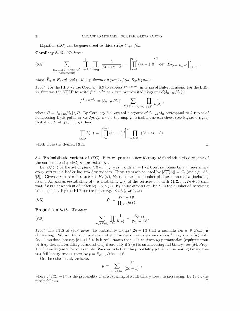
Equation (EC) can be generalized to thick strips δn+2k/δn.
Corollary 8.12. We have:
(8.4)∑
(p1,...,pk)∈Dyck(n)k
noncrossing
k∏r=1
∏(a,b)∈pr
1
2b+ 4r − 3=
[k−1∏r=1
(4r − 1)!!
]2
det[E2(n+i+j)−3
]ki,j=1
,
where En = En/n! and (a, b) ∈ p denotes a point of the Dyck path p.
Proof. For the RHS we use Corollary 8.9 to express fδn+2k/δn in terms of Euler numbers. For the LHS,we first use the NHLF to write fδn+2k/δn as a sum over excited diagrams E(δn+2k/δn) :
fδn+2k/δn = |δn+2k/δn|!∑
D∈E(δn+2k/δn)
∏u∈D
1
h(u),
where D = [δn+2k/δn] \D. By Corollary 8.4, excited diagrams of δn+2k/δn correspond to k-tuples ofnoncrossing Dyck paths in FanDyck(k, n) via the map ϕ. Finally, one can check (see Figure 6 right)that if ϕ : D 7→ (p1, . . . , pk) then∏
u∈Dh(u) =
[ k−1∏r=1
(4r − 1)!!
]2 ∏(a,b)∈pr
(2b+ 4r − 3) ,
which gives the desired RHS. �
8.4. Probabilistic variant of (EC). Here we present a new identity (8.6) which a close relative ofthe curious identity (EC) we proved above.
Let BT (n) be the set of plane full binary trees τ with 2n+ 1 vertices, i.e. plane binary trees whereevery vertex is a leaf or has two descendants. These trees are counted by |BT (n)| = Cn (see e.g. [S5,§2]). Given a vertex v in a tree τ ∈ BT (n), h(v) denotes the number of descendants of v (includingitself). An increasing labelling of τ is a labelling ω(·) of the vertices of τ with {1, 2, . . . , 2n+ 1} suchthat if u is a descendant of v then ω(v) ≤ ω(u). By abuse of notation, let fτ is the number of increasinglabelings of τ . By the HLF for trees (see e.g. [Sag3]), we have:
(8.5) fτ =(2n+ 1)!∏v∈τ h(v)
.
Proposition 8.13. We have:
(8.6)∑
τ∈BT (n)
∏v∈τ
1
h(v)=
E2n+1
(2n+ 1)!.
Proof. The RHS of (8.6) gives the probability E2n+1/(2n + 1)! that a permutation w ∈ S2n+1 isalternating. We use the representation of a permutation w as an increasing binary tree T (w) with2n+ 1 vertices (see e.g. [S4, §1.5]). It is well-known that w is an down-up permutation (equinumerouswith up-down/alternating permutations) if and only if T (w) is an increasing full binary tree [S4, Prop.1.5.3]. See Figure 7 for an example. We conclude that the probability p that an increasing binary treeis a full binary tree is given by p = E2n+1/(2n+ 1)!.
On the other hand, we have:
p =∑
τ∈BT (n)
fτ
(2n+ 1)!,
where fτ/(2n+ 1)! is the probability that a labelling of a full binary tree τ is increasing. By (8.5), theresult follows. �
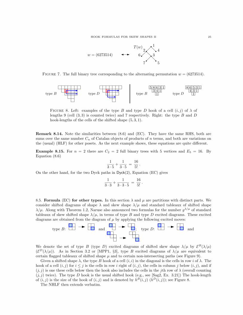
HOOK FORMULAS FOR SKEW SHAPES II 25
w = (6273514)
12
6 3
7 5
4T (w)
Figure 7. The full binary tree corresponding to the alternating permutation w = (6273514).
14
81135
36
13
51136
48
type B type D type B type D
Figure 8. Left: examples of the type B and type D hook of a cell (i, j) of λ oflengths 9 (cell (3, 3) is counted twice) and 7 respectively. Right: the type B and Dhook-lengths of the cells of the shifted shape (5, 3, 1).
Remark 8.14. Note the similarities between (8.6) and (EC). They have the same RHS, both aresums over the same number Cn of Catalan objects of products of n terms, and both are variations onthe (usual) (HLF) for other posets. As the next example shows, these equations are quite different.
Example 8.15. For n = 2 there are C2 = 2 full binary trees with 5 vertices and E5 = 16. ByEquation (8.6)
1
3 · 5 +1
3 · 5 =16
5!.
On the other hand, for the two Dyck paths in Dyck(2), Equation (EC) gives
1
3 · 3 +1
3 · 3 · 5 =16
5!.
8.5. Formula (EC) for other types. In this section λ and µ are partitions with distinct parts. Weconsider shifted diagrams of shape λ and skew shape λ/µ and standard tableaux of shifted shapeλ/µ. Along with Theorem 1.2, Naruse also announced two formulas for the number gλ/µ of standardtableaux of skew shifted shape λ/µ, in terms of type B and type D excited diagrams. These exciteddiagrams are obtained from the diagram of µ by applying the following excited moves:
type B: and ; type D: and
.
We denote the set of type B (type D) excited diagrams of shifted skew shape λ/µ by EB(λ/µ)(ED(λ/µ)). As in Section 3.2 or [MPP1, §3], type B excited diagrams of λ/µ are equivalent tocertain flagged tableaux of shifted shape µ and to certain non-intersecting paths (see Figure 9).
Given a shifted shape λ, the type B hook of a cell (i, i) in the diagonal is the cells in row i of λ. Thehook of a cell (i, j) for i ≤ j is the cells in row i right of (i, j), the cells in column j below (i, j), and if(j, j) is one these cells below then the hook also includes the cells in the jth row of λ (overall counting(j, j) twice). The type D hook is the usual shifted hook (e.g., see [Sag2, Ex. 3.21]) The hook-lengthof (i, j) is the size of the hook of (i, j) and is denoted by hB(i, j) (hD(i, j)); see Figure 8.
The NHLF then extends verbatim.
26 ALEJANDRO MORALES, IGOR PAK, GRETA PANOVA
Theorem 8.16 (Naruse [Naru]). Let λ, µ be partitions with distinct parts, such that µ ⊂ λ. We have
gλ/µ = |λ/µ|!∑
S∈EB(λ/µ)
∏(i,j)∈[λ]\S
1
hB(i, j),(8.7)
= |λ/µ|!∑
S∈ED(λ/µ)
∏(i,j)∈[λ]\S
1
hD(i, j),(8.8)
where hB(i, j) and hD(i, j) are the shifted hook-lengths of type B and type D, respectively.
Example 8.17 (shifted thick zigzag strip). The shifted analogue of the staircase is the trapezoid∇n = (2n− 1, 2n− 3, . . . , 1). The analogue of the thick strip is the shifted skew shape ∇n+k/∇n. Thenumber of type B excited diagrams of this shape has a product formula analogous to (8.1).
Proposition 8.18.
(8.9) |EB(∇n+k/∇n)| =k∏h=1
n∏i=1
n∏j=1
h+ i+ j − 1
h+ i+ j − 2.
Proof. As in the standard shape case, the type B excited diagrams correspond to shifted flaggedtableaux of trapezoid shape ∇n with entries in row i ≤ i+ k. By subtracting i to all entries in row iof such tableaux they are equivalent to plane partitions of trapezoid shape ∇n with entries ≤ k. Bya result of Proctor [Pro], recently proved bijectively in [HPPW], these are equinumerous with planepartitions in a n × n × k box (see also [HW]). Thus, by MacMahon’s boxed plane partition formulathe result follows. �
In the case k = 1 we obtain |EB(∇n+1/∇n)| =(
2nn
)(see Figure 9). When k = n, |EB(∇2n/∇n)|
counts the number of plane partitions that fit inside the n× n× n box (see e.g. [OEIS, A08793]).
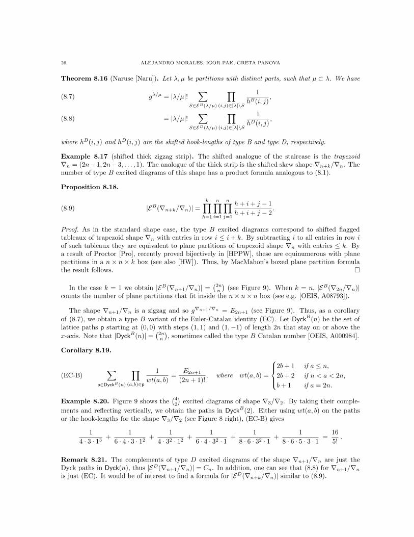
The shape ∇n+1/∇n is a zigzag and so g∇n+1/∇n = E2n+1 (see Figure 9). Thus, as a corollary
of (8.7), we obtain a type B variant of the Euler-Catalan identity (EC). Let DyckB(n) be the set oflattice paths p starting at (0, 0) with steps (1, 1) and (1,−1) of length 2n that stay on or above the
x-axis. Note that |DyckB(n)| =(
2nn
), sometimes called the type B Catalan number [OEIS, A000984].
Corollary 8.19.
(EC-B)∑
p∈DyckB(n)
∏(a,b)∈p
1
wt(a, b)=
E2n+1
(2n+ 1)!, where wt(a, b) =
2b+ 1 if a ≤ n,2b+ 2 if n < a < 2n,
b+ 1 if a = 2n.
Example 8.20. Figure 9 shows the(
42
)excited diagrams of shape ∇3/∇2. By taking their comple-
ments and reflecting vertically, we obtain the paths in DyckB(2). Either using wt(a, b) on the pathsor the hook-lengths for the shape ∇3/∇2 (see Figure 8 right), (EC-B) gives
1
4 · 3 · 13+
1
6 · 4 · 3 · 12+
1
4 · 32 · 12+
1
6 · 4 · 32 · 1 +1
8 · 6 · 32 · 1 +1
8 · 6 · 5 · 3 · 1 =16
5!.
Remark 8.21. The complements of type D excited diagrams of the shape ∇n+1/∇n are just theDyck paths in Dyck(n), thus |ED(∇n+1/∇n)| = Cn. In addition, one can see that (8.8) for ∇n+1/∇nis just (EC). It would be of interest to find a formula for |ED(∇n+k/∇n)| similar to (8.9).
HOOK FORMULAS FOR SKEW SHAPES II 27
1 12
1 22
1 13
1 23
2 23
1 1 1 1 1 2 23
2
Figure 9. Correspondence between type B excited diagrams in ∇3/∇2, paths in
DyckB(2) and flagged tableaux of shape ∇2 with flag (2, 3).
8.6. q-analogue of Euler numbers via SSYT. We use our first q-analogue of NHLF (Theorem 1.3)to obtain identities for sδn+2k/δn(1, q, q2, . . .) in terms of Dyck paths.
Proof of Corollary 1.7. By Theorem 1.3 for the skew shape δn+2/δn and (8.2) we have
(8.10)E2n+1(q)
(1− q)(1− q2) · · · (1− q2n+1)=
∑D∈E(δn+2/δn)
∏(i,j)∈[δn+2]\D
qλ′j−i
1− qh(i,j).
Let D in E(δn+2/δn) corresponds to the Dyck path p and cell (i, j) in D corresponds to point (a, b) inp then h(i, j) = 2b+ 1 and λ′j − i = b. Using this correspondence, the LHS of (8.10) becomes the LHSof the desired expression. �
Corollary 8.22.
∑(p1,...,pk)∈Dyck(n)k
noncrossing
k∏r=1
∏(a,b)∈pr
qb+2r−2
1− q2b+4r−3=
(k−1∏r=1
[4r − 1]!!
)2
det[E2(n+i+j)−3(q)
]ki,j=1
where En(q) := En(q)/(1− q)(1− q2) · · · (1− qn) and [2m− 1]!! := (1− q)(1− q3) · · · (1− q2m−1).
Proof. For the LHS, use Corollary 8.8 to express sδn+2k/δn(1, q, q2, . . .) in terms of q-Euler polynomials
Em(q). For the RHS, first use Theorem 1.3 for the skew shape δn+2k/δn and then follow the sameargument as that of Corollary 8.12. �
Remark 8.23. Combinatorial proofs of Corollary 1.6 and Corollary 1.7 are obtained from the proof inSection 5 of (NHLF). Similarly, combinatorial proofs of Corollary 8.12 and Corollary 8.22 are obtainedfrom the proof in Section 5 of (NHLF) and the first q-NHLF for all shapes, or from Konvalinka’sbijective proof of (NHLF) in [Kon] and the first q-NHLF for border strips.2
9. Pleasant diagrams and RPP of border strips and thick strips
In this section we study pleasant diagrams in P(δn+2/δn) and our second q-analogue of NHLF (The-orem 1.4) for RPP of shape δn+2/δn. Recall that p(λ/µ) denotes the number of pleasant diagrams ofshape λ/µ.
9.1. Pleasant diagrams and Schroder numbers. Let sn be the n-th Schroder number [OEIS,A001003] which counts lattice paths from (0, 0) to (2n, 0) with steps (1, 1), (1,−1), and (2, 0) thatnever go below the x-axis and no steps (2, 0) on the x-axis.
Theorem 9.1. We have: p(δn+2/δn) = 2n+2sn , for all n ≥ 1.

28 ALEJANDRO MORALES, IGOR PAK, GRETA PANOVA
27 26 26 25 26
Figure 10. Each Dyck path p of size n with m excited peaks (denoted in gray) yields22n−m+2 pleasant diagrams. For n = 3, we have C5 = 5 and s3 = 11. Thus, there are|E(δ3+2/δ3)| = C3 = 5 excited diagrams and p(δ3+2/δ3) = 25s3 = 352 pleasantdiagrams.
The proof is based on the following corollary which is in turn a direct application of Theorem 4.3.A high peak of a Dyck path p is a peak of height strictly greater than one. We denote by HP(p) theset of high peaks of p, and by NP(p) the points of the path that are not high peaks. We use 2S denotethe set of subsets of S.
Corollary 9.2. The pleasant diagrams in P(δn+2/δn) are in bijection with⋃p∈Dyck(n)
(HP(p)× 2NP(p)
).
Proof. By Corollary 8.4 for the zigzag strip δn+2/δn we have NI(δn+2/δn) is the set of Dyck pathsDyck(n). Then by Theorem 4.3, we have:
P(δn+2/δn) =⋃
p∈Dyck(n)
(Λ(p)× 2p\Λ(p)
).
Lastly, note that the excited peaks of a Dyck path are exactly the high peaks so Λ(p) = HP(p) andp \ Λ(p) = NP(p). �
Proof of Theorem 9.1. It is known (see [Deu]), that the number of Dyck paths of size n with k−1 highpeaks equals the Narayana number N(n, k) = 1
n
(nk
)(nk−1
). On the other hand, Schroder numbers sn
can be written as
(9.1) sn =
n∑k=1
N(n, k)2k−1
(see e.g. [Sul]). By Lemma 9.2, we have:
(9.2) p(δn+2/δn) =∑
p∈Dyck(n)
2|NP(p)| .
Suppose Dyck path γ has k − 1 peaks, 1 ≤ k ≤ n. Then |NP(γ)| = 2n + 1 − (k − 1). Therefore,equation (9.2) becomes
p(δn+2/δn) = 2n+2n∑k=1
N(n, k)2n−k = 2n+2n∑k=1
N(n, n− k + 1)2n−k = 2n+2sn ,
where we use the symmetry N(n, k) = N(n, n− k + 1) and (9.1). �
In the same way as |E(δn+2k/δn)| is given by a determinant of Catalan numbers, preliminary com-putations suggest that p(δn+2k/δn) is given by a determinant of Schroder numbers.
Conjecture 9.3. We have: p(δn+4/δn) = 22n+5(snsn+2 − s2n+1). More generally, for all k ≥ 1, we
have:p(δn+2k/δn) = 2(k2) det
[sn−2+i+j
]ki,j=1
, where sn = 2n+2sn .
2Jang Soo Kim has a direct proof of Corollary 1.7 using continued fractions and orthogonal polynomials (private
communication).
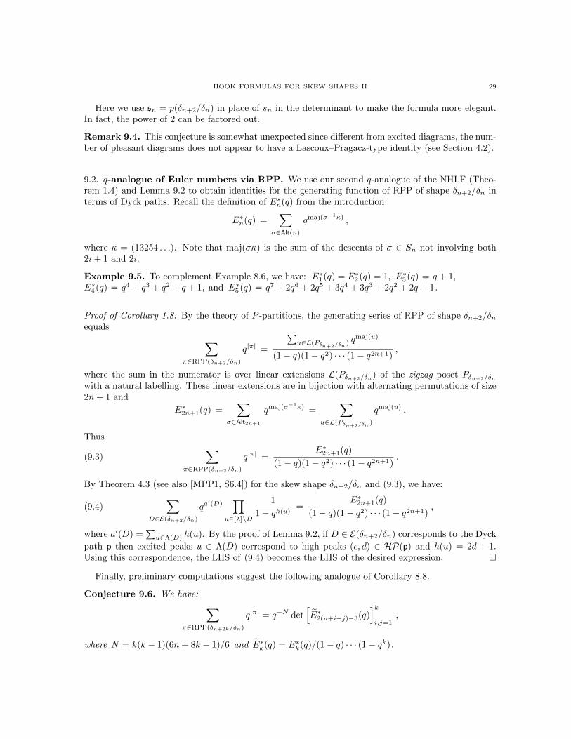
HOOK FORMULAS FOR SKEW SHAPES II 29
Here we use sn = p(δn+2/δn) in place of sn in the determinant to make the formula more elegant.In fact, the power of 2 can be factored out.
Remark 9.4. This conjecture is somewhat unexpected since different from excited diagrams, the num-ber of pleasant diagrams does not appear to have a Lascoux–Pragacz-type identity (see Section 4.2).
9.2. q-analogue of Euler numbers via RPP. We use our second q-analogue of the NHLF (Theo-rem 1.4) and Lemma 9.2 to obtain identities for the generating function of RPP of shape δn+2/δn interms of Dyck paths. Recall the definition of E∗n(q) from the introduction:
E∗n(q) =∑
σ∈Alt(n)
qmaj(σ−1κ) ,
where κ = (13254 . . .). Note that maj(σκ) is the sum of the descents of σ ∈ Sn not involving both2i+ 1 and 2i.
Example 9.5. To complement Example 8.6, we have: E∗1 (q) = E∗2 (q) = 1, E∗3 (q) = q + 1,E∗4 (q) = q4 + q3 + q2 + q + 1, and E∗5 (q) = q7 + 2q6 + 2q5 + 3q4 + 3q3 + 2q2 + 2q + 1.
Proof of Corollary 1.8. By the theory of P -partitions, the generating series of RPP of shape δn+2/δnequals ∑
π∈RPP(δn+2/δn)
q|π| =
∑u∈L(Pδn+2/δn
) qmaj(u)
(1− q)(1− q2) · · · (1− q2n+1),
where the sum in the numerator is over linear extensions L(Pδn+2/δn) of the zigzag poset Pδn+2/δn
with a natural labelling. These linear extensions are in bijection with alternating permutations of size2n+ 1 and
E∗2n+1(q) =∑
σ∈Alt2n+1
qmaj(σ−1κ) =∑
u∈L(Pδn+2/δn)
qmaj(u) .
Thus
(9.3)∑
π∈RPP(δn+2/δn)
q|π| =E∗2n+1(q)
(1− q)(1− q2) · · · (1− q2n+1).
By Theorem 4.3 (see also [MPP1, S6.4]) for the skew shape δn+2/δn and (9.3), we have:
(9.4)∑
D∈E(δn+2/δn)
qa′(D)
∏u∈[λ]\D
1
1− qh(u)=
E∗2n+1(q)
(1− q)(1− q2) · · · (1− q2n+1),
where a′(D) =∑u∈Λ(D) h(u). By the proof of Lemma 9.2, if D ∈ E(δn+2/δn) corresponds to the Dyck
path p then excited peaks u ∈ Λ(D) correspond to high peaks (c, d) ∈ HP(p) and h(u) = 2d + 1.Using this correspondence, the LHS of (9.4) becomes the LHS of the desired expression. �
Finally, preliminary computations suggest the following analogue of Corollary 8.8.
Conjecture 9.6. We have: ∑π∈RPP(δn+2k/δn)
q|π| = q−N det[E∗2(n+i+j)−3(q)
]ki,j=1
,
where N = k(k − 1)(6n+ 8k − 1)/6 and E∗k(q) = E∗k(q)/(1− q) · · · (1− qk) .
30 ALEJANDRO MORALES, IGOR PAK, GRETA PANOVA
10. Final remarks
10.1. Other known formulas for fλ/µ are the Jacobi–Trudi identity, the Littlewood–Richardson rule,and the Okounkov–Olshanski formula [OO]. We discuss these and other less known formulas for fλ/µ
coming from equivariant Schubert structure constants in [MPP1, §9].The Jacobi-Trudi identity is one of the first nontrivial formulas to count fλ/µ. In this paper we have
unveiled a strong relation between the Lascoux–Pragacz identity for Schur functions and the NHLFfor fλ/µ. As mentioned in Section 7.5, Hamel and Goulden [HaG] unified these two identities intoan exponential family of determinantal identities of Schur functions. Chen–Yan–Yang [CYY] gave amethod to transform among these identities. It would be of interest if other formulas for fλ/µ, likethe ones mentioned above, are related to special cases of Hamel–Goulden identities.
10.2. In [Kon], Konvalinka gives a new proof of the NHLF. Specifically, he presents a bumpingalgorithm on bicolored flagged tableaux of shape µ to prove the Pieri–Chevalley formula for generalskew shapes (see [IN, §8.4] and [MPP2]). For the border strips this approach is different from ourproof of Lemma 6.1. In fact, our proof uses the underlying single path in the excited diagrams of aborder strip to perform cancelations. While Konvanlinka’s proof is substraction-free, it involves aninsertion on the inner partition µ that could be arbitrary even for a border strip.
It is worth noting that both proofs of Lemma 5.1 are quite technical. Initially, this came as a surpriseto us, and our effort to understand the underlying multivariate algebraic identities led to [MPP2]. Letus also mention that in [IN], the authors use the Pieri–Chevalley formula for Kostant polynomials toprove the analogue of Lemma 6.1 for all skew shapes.
10.3. There is a very large literature on alternating permutations, Euler numbers, Dyck paths, Cata-lan and Schroder numbers, which are some of the classical combinatorial objects and sequences. Werefer to [S3] for the survey on the first two, to [S5] for a thorough treatment of the last three, andto [GJ, OEIS, S4] for various generalizations, background and further references.
Finally, the first q-analogue En(q) of Euler numbers we consider is standard in the literature andsatisfies a number of natural properties, including a q-version of equation (1.1) (see e.g. [GJ, §4.2]).However, the second q-analogue E∗n(q) appears to be new. It would be interesting to see how it fits withthe existing literature of multivariate Euler polynomials and statistics on alternating permutations.
10.4. The curious Catalan determinant in Corollary 8.3 appeared in the first arXiv version of [MPP1].However, the proof here is more self contained as a direct application of Theorem 3.3. This Catalandeterminant is both similar and related3 to another Catalan determinant in [AL, proof of Lemma 1.1].In fact, both determinants are special cases of more general counting results, and both can be provedby the Lindstrom–Gessel–Viennot lemma.
10.5. The connection between alternating permutations and symmetric functions of border strips goesback to Foulkes [Fou], and has been repeatedly generalized and explored ever since (see [S3]). It isperhaps surprising that Corollary 1.6 is so simple, since the other two positive formulas in Section 10.1become quite involved. For the LR-coefficients, let partition ν ` 2n+ 1 be such that ν1, `(ν) ≤ n+ 1.
It is easy to see that in this case the corresponding LR-coefficient is nonzero: cδn+2
δn ν> 0, suggesting
that summation over all such ν would can be hard to compute.
10.6. The proof in [MPP1] of the skew RPP q-analogue of Naruse (Theorem 1.4) is already bijectiveusing the Hillman–Grassl correspondence. It would be interesting to see if for RPP the case for borderstrips implies the case for all connected skew shapes. Note that we do not know of a Lascoux–Pragaczanalogue of (5.7) for skew RPP. Such an identity might not exists since the number of pleasant diagrams(the supports of arrays obtained from Hillman–Grassl applied to skew RPP) does not appear to have aLascoux–Pragacz type identity as discussed in Section 4.2. On the other hand, Conjecture 9.3 suggeststhat there might be such a formula in some cases.
3The connection was found by T. Amdeberhan (personal communication).

HOOK FORMULAS FOR SKEW SHAPES II 31
Acknowledgements. We are grateful to Per Alexandersson, Dan Betea, Sara Billey, Jang Soo Kim,Matjaz Konvalinka, Leo Petrov, Eric Rains, Luis Serrano, Richard Stanley and Alex Yong for usefulcomments and help with the references. We are also thankful to Tewodros Amdeberhan, BrendonRhoades and Emily Leven for discussions on the curious Catalan determinants. The first author issupported by an AMS-Simons travel grant. The second and third authors were partially supported bythe NSF.
References
[AR] R. Adin and Y. Roichman, Standard Young tableaux, in Handbook of Enumerative Combinatorics (M. Bona,
editor), CRC Press, Boca Raton, 2015, 895–974.
[AL] T. Amdeberhan and E. Leven, Multi-cores, posets, and lattice paths, Adv. Appl. Math. 71 (2015), 1–13.[AJS] H.H. Andersen, J.C. Jantzen and W. Soergel, Representations of quantum groups at p-th root of unity and of
semisimple groups in characteristic p: independence of p, Asterisque, 220, 321.
[BR] Y. Baryshnikov and D. Romik, Enumeration formulas for Young tableaux in a diagonal strip, Israel J. Math.178 (2010), 157–186.
[BGR] A. Borodin, V. Gorin and E. M. Rains, q-distributions on boxed plane partitions, Selecta Math. 16 (2010),
731–789.[CYY] W. Y. C. Chen, A. L. B. Yan and G.-G. Yang, Transformations of border strips and Schur function determi-
nants, J. Algebraic Combin. 21 (2005), 379–394.
[SV] M. de Sainte-Catherine and X. G. Viennot, Enumeration of certain Young tableaux with bounded height, inLecture Notes Math. 1234, Springer, Berlin, 1986, 58–67.
[Deu] E. Deutsch, An involution on Dyck paths and its consequences, Discrete Math. 204 (1999), 163–166.[Eli] S. Elizalde, A bijection between 2-triangulations and pairs of non-crossing Dyck paths, J. Combin. Theory,
Ser. A 114 (2007), 1481–1503.
[Fis] I. Fischer, A bijective proof of the hook-length formula for shifted standard tableaux, arXiv:math/0112261.[FK] S. Fomin, A.N. Kirillov, Reduced words and plane partitions, J. of Algebraic Combin. 6 (1997), 311–319.
[Fou] H. O. Foulkes, Tangent and secant numbers and representations of symmetric groups, Discrete Math. 15
(1976), 311–324.[FRT] J. S. Frame, G. de B. Robinson and R. M. Thrall, The hook graphs of the symmetric group, Canad. J. Math. 6
(1954), 316–324.
[GV] I. M. Gessel and X. G. Viennot, Determinants, paths and plane partitions, preprint (1989); available attinyurl.com/zv3wvyh.
[GJ] I. P. Goulden and D. M. Jackson, Combinatorial enumeration, John Wiley, New York, 1983.
[GK] W. Graham and V. Kreiman, Excited Young diagrams, equivariant K-theory, and Schubert varieties, Trans.AMS 367 (2015), 6597–6645.
[GNW] C. Greene, A. Nijenhuis and H. S. Wilf, A probabilistic proof of a formula for the number of Young tableauxof a given shape, Adv. Math. 31 (1979), 104–109.
[HW] Z. Hamaker and N. Williams, Subwords and plane partitions, Proceedings FPSAC 2015, 241–252.
[HPPW] Z. Hamaker, R. Patrias, O. Pechenik, and N. Williams, Doppelgangers: bijections of plane partitions,arXiv:1602.05535.
[HaG] A. M. Hamel and I. P. Goulden, Planar decompositions of tableaux and Schur function determinants, European
J. Combin. 16 (1995), 461–477.[HiG] A. P. Hillman and R. M. Grassl, Reverse plane partitions and tableau hook numbers, J. Combin. Theory,
Ser. A 21 (1976), 216–221.[IN] T. Ikeda and H. Naruse, Excited Young diagrams and equivariant Schubert calculus, Trans. AMS 361 (2009),
5193–5221.
[Jin] E.Y. Jin, Outside nested decompositions of skew diagrams of skew diagrams and Schur functions determinants,
arXiv:1606.01764
[Jon] J. Jonsson, Generalized triangulations and diagonal-free subsets of stack polyominoes, J. Combin. Theory,
Ser. A 112 (2005), 117–142.[K1] C. Krattenthaler, Bijective proofs of the hook formulas for the number of standard Young tableaux, ordinary
and shifted, Electron. J. Combin. 2 (1995), RP 13, 9 pp.
[Kon] M. Konvalinka, A bijective proof of the hook-length formula for skew shapes, preprint 2016.[Kre1] V. Kreiman, Schubert classes in the equivariant K-theory and equivariant cohomology of the Grassmannian,
arXiv:math.AG/0512204.
[Kre2] V. Kreiman, Schubert classes in the equivariant K-theory and equivariant cohomology of the LagrangianGrassmannian, arXiv:math.AG/0602245.
[LasP] A. Lascoux and P. Pragacz, Ribbon Schur functions, European J. Combin. 9 (1988), 561–574.

32 ALEJANDRO MORALES, IGOR PAK, GRETA PANOVA
[MPP1] A.H. Morales, I. Pak and G. Panova, Hook formulas for skew shapes I. q-analogues and bijections,
arXiv:1512.08348.[MPP2] A.H. Morales, I. Pak and G. Panova, Hook formulas for skew shapes III. Multivariate formulas from Schubert
calculus, in preparation.
[MPP3] A.H. Morales, I. Pak and G. Panova, Hook formulas for skew shapes IV. Increasing tableaux and factorialGrothendieck polynomials, in preparation.
[MS] A. I. Molev and B. E. Sagan, A Littlewood-Richardson rule for factorial Schur functions, Trans. AMS 351(1999), 4429–4443.
[Naru] H. Naruse, Schubert calculus and hook formula, talk slides at 73rd Sem. Lothar. Combin., Strobl, Austria,
2014; available at tinyurl.com/z6paqzu.[NPS] J.-C. Novelli, I. Pak and A. V. Stoyanovskii, A direct bijective proof of the hook-length formula, Discrete
Math. Theor. Comput. Sci. 1 (1997), 53–67.
[OO] A. Okounkov and G. Olshanski, Shifted Schur functions, St. Petersburg Math. J. 9 (1998), 239–300.[Pak] I. Pak, Hook length formula and geometric combinatorics. Sem. Lothar. Combin. 46 (2001), Art. B46f, 13 pp.
[Pro] R. A. Proctor, Shifted plane partitions of trapezoidal shape. Proc. AMS 89 (1983), 553–559.
[Rem] J. B. Remmel, Bijective proofs of formulae for the number of standard Young tableaux, Linear and MultilinearAlgebra 11 (1982), 45–100.
[Sag1] B. E. Sagan, Enumeration of partitions with hooklengths, European J. Combin. 3 (1982), 85–94.
[Sag2] B. E. Sagan, The Symmetric Group, Springer, 2000.[Sag3] B. E. Sagan, Probabilistic proofs of hook length formulas involving trees, Sem. Lothar. Combin. 61A (2009),
Art. B61Ab, 10 pp.[Sage] The Sage-Combinat community. Sage-Combinat: enhancing Sage as a toolbox for computer exploration in
algebraic combinatorics, 2013. http://combinat.sagemath.org.
[SS] L. Serrano and C. Stump, Maximal fillings of moon polyominoes, simplicial complexes, and Schubert polyno-mials, Electron. J. Combin. 19 (2012), RP 16, 18 pp.
[OEIS] N. J. A. Sloane, The Online Encyclopedia of Integer Sequences, oeis.org.
[S1] R. P. Stanley, Theory and applications of plane partitions, Part 2, Stud. Appl. Math. 50 (1971), 259–279.[S2] R. P. Stanley, Plane partitions, past, present, and future, Proceedings Third International Conference (New
York 1985), 397–401.
[S3] R. P. Stanley, A survey of alternating permutations, in Combinatorics and graphs, AMS, Providence, RI, 2010,165–196.
[S4] R. P. Stanley, Enumerative Combinatorics, vol. 1 (second ed.) and vol. 2 (first ed.), Cambridge Univ. Press,
2012 and 1999.[S5] R. P. Stanley, Catalan Numbers, Cambridge Univ. Press, 2015.
[Sul] R. A. Sulanke, The Narayana distribution, J. Statist. Plann. Inference 101 (2002), 311–326.
[Wac] M. Wachs, Flagged Schur functions, Schubert polynomials, and symmetrizing operators, J. Combin. Theory,Ser. A 40 (1985), 276–289.
[Zei] D. Zeilberger, A short hook-lengths bijection inspired by the Greene–Nijenhuis–Wilf proof, Discrete Math. 51(1984), 101–108.