Hong Su, Ph.D. Summitech Engineering, Inc. Virtual ... · Virtual Automotive Product Development...

Hong Su, Ph.D. Summitech Engineering, Inc. Virtual Automotive Product Development Using Frequency Domain Simulation Techniques

Technical BackgroundTime vs. frequency domainFrequency characteristics Frequency response analysis

Durability virtual testsDynamic loadsStructural durability evaluation

NVH virtual testsVibration response performanceAcoustic and noise performance

Conclusions

Virtual Automotive Product Development Using Frequency Domain Simulation Techniques

Data in Time and Frequency Domains

Frequency domain PSD data

Time domain data Same Vehicle load Data

But in different domainsRelated by FFT techniqueAs Fourier transform pairs

( ) ( ) ( )[ ] ( ) ( )dttxtxT

limtxtxERT

Tτττ +=+= ∫∞→ 0

1

( ) ( ) ττω ωτ deRS i−∞

∞−∫=

( ) ( ) ωωπ

τ ωτ deSR i∫∞

∞−=

21

Example: PG Belgium Block Road

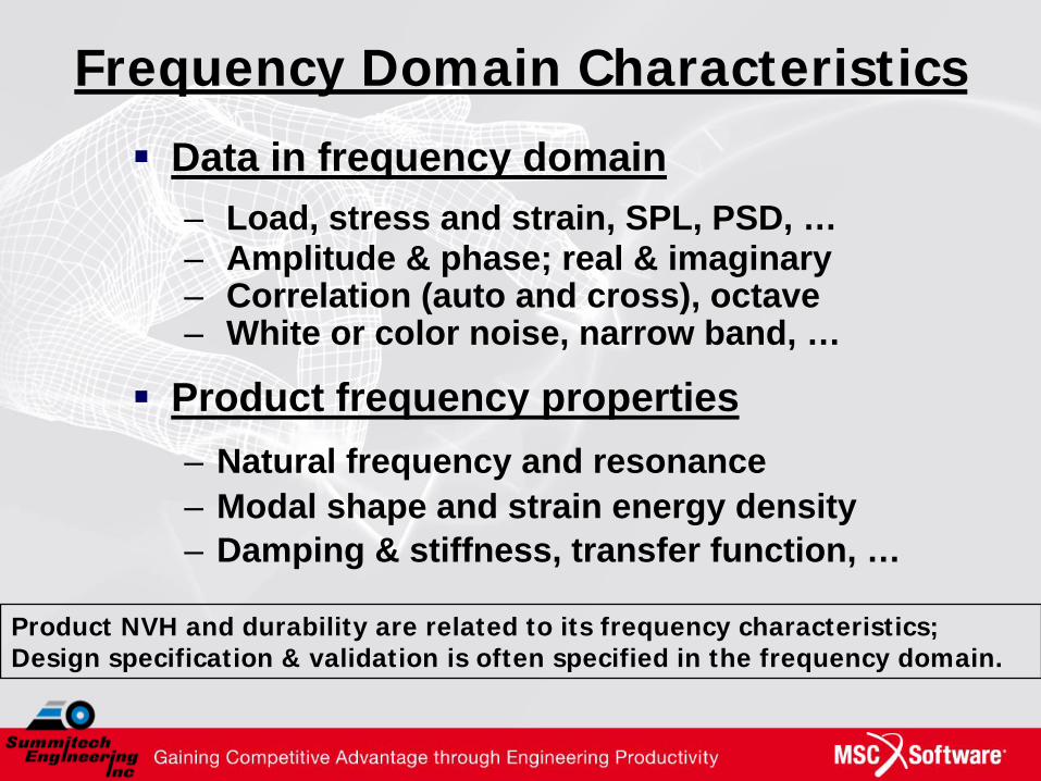
Frequency Domain Characteristics

Data in frequency domain– Load, stress and strain, SPL, PSD, …– Amplitude & phase; real & imaginary– Correlation (auto and cross), octave – White or color noise, narrow band, …

Product frequency properties– Natural frequency and resonance – Modal shape and strain energy density– Damping & stiffness, transfer function, …

Product NVH and durability are related to its frequency characteristics;Design specification & validation is often specified in the frequency domain.

Product Performance SimulationsTime domain simulation

0A system of nonlinear differential equations0Solve for response {x(t)} in time steps

Frequency domain simulation

0A system of localized linear algebra equations0Solve for response {X(w)} in frequency points

[ ] ( ){ } ( )[ ] ( ){ } ( )[ ] ( ){ } ( ){ }tptxTxxKtxTxxCtxM =++ ,,,, &&&&&

( ){ } ( )[ ] ( ){ }ωωω PHX ⋅=

( )[ ] [ ] ( )[ ] ( )[ ]( ) 12 ,,,,,, −++−= jleqjleq PTXKPTXCiMH ωωωωω

2G 4G 8G

Cold Case (-40C)

{i[C]w+([K]-[M]w 2̂)}, 2g_cold

{i[C]w+([K]-[M]w 2̂)}, 4g_cold

{i[C]w+([K]-[M]w^2)}, 8g_cold

Ambient (23C)

{i[C]w+([K]-[M]w 2̂)}, 2g_room

{i[C]w+([K]-[M]w 2̂)}, 4g_room

{i[C]w+([K]-[M]w^2)}, 8g_room

Hot Case (120C)

{i[C]w+([K]-[M]w 2̂)}, 2g_hot

{i[C]w+([K]-[M]w 2̂)}, 4g_hot

{i[C]w+([K]-[M]w^2)}, 8g_hot

Vibration Load LevelTemperature Case

Example: Localized Nonlinear FE Model (An Array of Local Models of An EIS)

( )[ ] [ ] ( )[ ] ( )[ ]( ) 12 ,,,,,, −++−= jleqjleq PTXKPTXCiMH ωωωωω

A system of localized linear equations in the frequency domain

Test conditions (I):

• Load level = 2g

• Temperatures:• Cold = -40ºC• Ambient = 23ºC• Hot = 120ºC

AIS Result Correlation, 2gzup1co

0.0

2.0

4.0

6.0

8.0

10.0

10 100 1000

Frequency (Hz)

Acc

e (g

)

Test

CAE

AIS Result Correlation, 2gzup1am

0.0

1.0

2.0

3.0

4.0

5.0

10 100 1000

Frequency (Hz)

Acc

e (g

)

Test

CAE

AIS Result Correlation, 2gzup1ht

0.0

1.0

2.0

3.0

10 100 1000

Frequency (Hz)

Acc

e (g

)

Test

CAE

Example: Localized Nonlinear FE Model EIS Assembly (Result Correlation I)

Test conditions (II):

• Load level = 4g

• Temperatures:• Cold = -40ºC• Ambient = 23ºC• Hot = 120ºC


0.0

2.0

4.0

6.0

8.0

10.0

10 100 1000

Frequency (Hz)

Acc

e (g

)

Test

CAE


0.0

2.0

4.0

6.0

8.0

10 100 1000

Frequency (Hz)

Acc

e (g

)

Test

CAE

AIS Result Corre la tion, 4gzup1ht

0.0

2.0

4.0

6.0

10 100 1000

Fre quency (Hz)

Acc

e (g

)

Test

CAE

Example: Localized Nonlinear FE Model EIS Assembly (Result Correlation II)

Test conditions (III):

h

Load level = 8g

h

Temperatures:h Cold = -40ºCh Ambient = 23ºCh Hot = 120ºC


0.0

5.0

10.0

15.0

20.0

10 100 1000

Frequency (Hz)

Acc

e (g

)

Test

CAE


0.0

4.0

8.0

12.0

16.0

10 100 1000

Frequency (Hz)

Acc

e (g

)

Test

CAE

AIS Result Correlation, 8gzup1ht

0.0

3.0

6.0

9.0

12.0

10 100 1000

Frequency (Hz)

Acc

e (g

)

Test

CAE

Example: Localized Nonlinear FE Model EIS Assembly (Result Correlation III)

A Flow Chart of CAE Virtual Tests (Frequency Domain)

KLT load level cases and temperature cases

Generate vibration load tables (Nastran)

Localized FE model H(K,C,ω), for case l,j

Generate SED matrix, hotspots

and FEM bulk data

Run frequency response simulation

(SOL111)

Yes: Process and sort element stress results

Evaluate structural fatigue damage

Engine load, environment and

duty cycles

CAD data: geometry and

BOM

Material S/N data

Set damage model and parameters

Output: Estimated

durability life

CAE material property database

Is the error acceptable?

No: Update model control

parameters

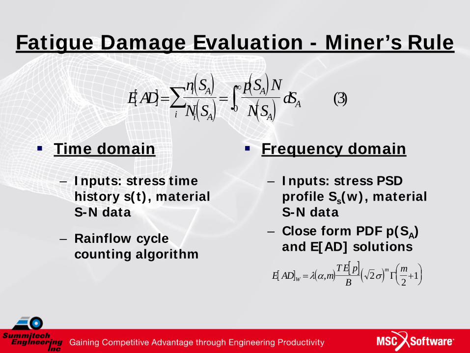
Fatigue Damage Evaluation - Miner’s Rule

Time domain

– Inputs: stress time history s(t), material S-N data

– Rainflow cycle counting algorithm

Frequency domain

– Inputs: stress PSD profile Ss (w), material S-N data

– Close form PDF p(SA ) and E[AD] solutions

[ ]( )( )

( )( )E AD

n SN S

pS NNS

dSi A

i Ai

A

AA= =∑ ∫

∞

03( )

[ ] ( ) [ ] ( )E AD mT E p

Bm

W

m= +

⎛⎝⎜

⎞⎠⎟λ α σ, 2

21Γ




Conclusions


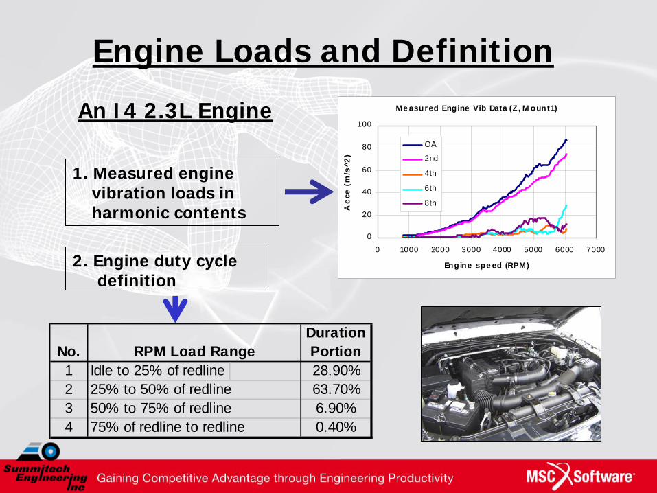
Engine Loads and Definition

2. Engine duty cycle definition

No.Duration Portion

1 Idle to 25% of redline 28.90%2 25% to 50% of redline 63.70%3 50% to 75% of redline 6.90%4 75% of redline to redline 0.40%

RPM Load Range

Me asured Engine Vib Data (Z , M ount1)

0

20

40

60

80

100

0 1000 2000 3000 4000 5000 6000 7000

Engine spe ed (RPM)

Acc

e (m

/s^2

)

OA

2nd

4th

6th

8th

An I4 2.3L Engine

1. Measured enginevibration loads in harmonic contents

Vibration Test Load Specification (Engine-mount Product, Random PSD format)

Test load specification based on1. Measured engine data 2. Duty cycle definition 3. Frequency analysis, and 4. Equivalent damage techniques

Random Vibration Load (Engine Mount)

1.0E-05

1.0E-04

1.0E-03

1.0E-02

1.0E-01

1.0E+00

10 100 1000

Frequency (Hz)

Acc

e PS

D (g

^2/H

z)

Frequency PSD(Hz) (g^2/Hz)

20 2.00E-0565 2.00E-01200 2.00E-01285 1.50E-031000 1.50E-03

RMS (g) = 5.7Test Duration = 100 hours

Ref: "Vibration Test Specification for Automotive Products," SAE Paper 2006-01-0729, by H. Su

Vibration Test Load Specification (Engine-mount Product, Swept Sine format)

Test load specification based on1. Measured engine data 2. Duty cycle definition 3. Frequency analysis, and 4. Equivalent damage techniques

Frequency Acceleration(Hz) (G)

20 1.165 9.56

200 9.56285 1.321000 1.32

Type of sweep = LogTime per sweep (min) = 20

Sweep speed (Oct/min) = 0.565Number of sweeps = 300

Test Duration (hours) = 100

Sine Vibration Load (Engine Mount, Z)

0

2

4

6

8

10

10 100 1000Frequency (Hz)

Acc

e (g

)

Left Mount

Rear Mount

Right Mount

Front Mount

FE Model of An Engine Suspension System

EM01 Rear-Bushing Dynamic Stiffness

0

100

200

300

400

500

600

700

800

0 200 400 600 800 1000

Frequency (Hz)St

iffne

ss (N

/mm

)

R-Direction

P-Direction

Q-Direction

EM01 Rear-Bushing Dynamic Damping

0.00

0.05

0.10

0.15

0.20

0 200 400 600 800 1000

Frequency (Hz)

Dam

ping

(N.s

/mm

)

R-Direction

P-Direction

Q-Direction

Nonlinear Rubber Bushing Damping Frequency Properties

Nonlinear Rubber Bushing Stiffness Frequency Properties

Suspended Engine and

TransmissionNonlinear rubber bushing properties are modeled by MSC.Nastran CBUSH elements and PBUSH tables

Durability Virtual Test of Engine Suspension

Sine Vibration Load (Engine Mount, Z)

0

2

4

6

8

10

10 100 1000

Frequency (Hz)

Acc

e (g

)

Bracket Stress Response

Engine Vibration Load Input

Right Mount Structure

Bracket Stress Distribution

Swept Sine Stress Response (E3017)

0

50

100

150

200

250

1 10 100 1000Frequency (Hz)

Stre

ss (M

Pa)

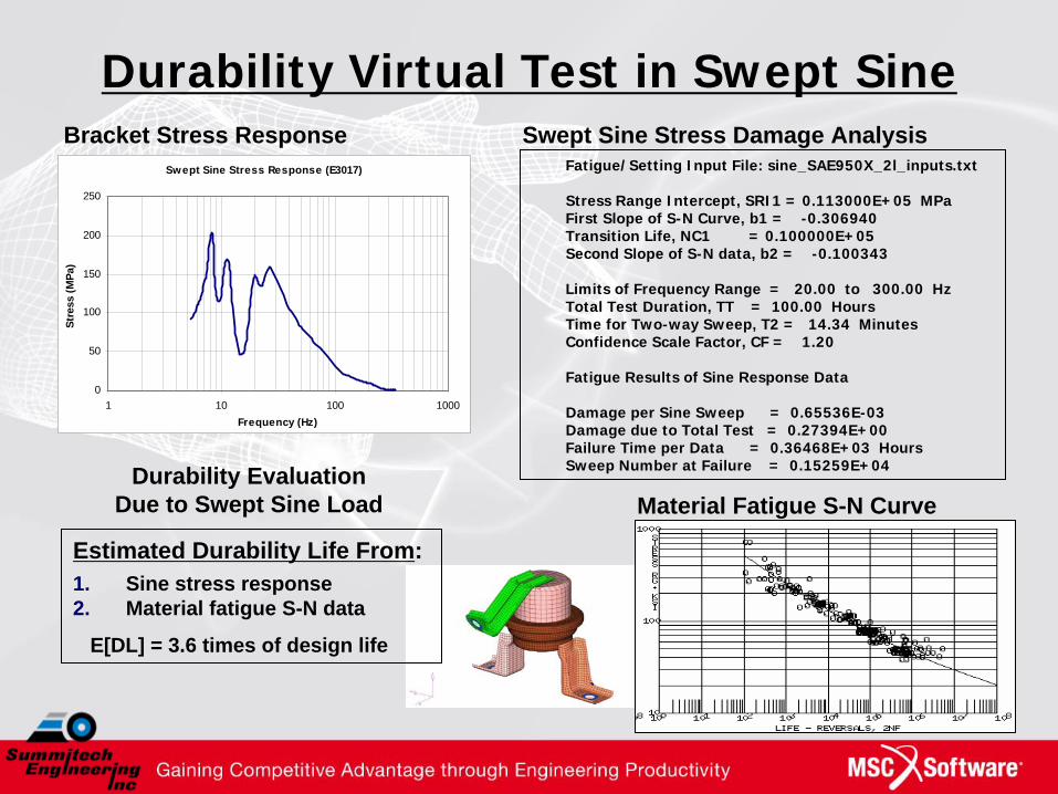
Durability Virtual Test in Swept SineBracket Stress Response

Material Fatigue S-N Curve

Estimated Durability Life From: 1. Sine stress response 2. Material fatigue S-N data

E[DL] = 3.6 times of design life

Fatigue/Setting Input File: sine_SAE950X_2l_inputs.txt

Stress Range Intercept, SRI1 = 0.113000E+05 MPaFirst Slope of S-N Curve, b1 = -0.306940Transition Life, NC1 = 0.100000E+05Second Slope of S-N data, b2 = -0.100343

Limits of Frequency Range = 20.00 to 300.00 HzTotal Test Duration, TT = 100.00 HoursTime for Two-way Sweep, T2 = 14.34 MinutesConfidence Scale Factor, CF = 1.20

Fatigue Results of Sine Response Data

Damage per Sine Sweep = 0.65536E-03Damage due to Total Test = 0.27394E+00Failure Time per Data = 0.36468E+03 HoursSweep Number at Failure = 0.15259E+04Durability Evaluation

Due to Swept Sine Load

Swept Sine Stress Damage AnalysisSwept Sine Stress Response (E3017)

0

50

100

150

200

250

1 10 100 1000Frequency (Hz)

Stre

ss (M

Pa)

Durability Virtual Test in Random PSD

Load: Power Hop HillPart: LR UCA BracketMaterial: SAE950XElement: 53691RMS = 55.08 MPaIrF, a = 0.412

Bracket stress response in PSDElement 53691 (Bracket, LR UCA (-Y))

1.E-01

1.E+00

1.E+01

1.E+02

1.E+03

1.E+04

1.E+05

0.01 0.10 1.00 10.00 100.00Frequency (Hz)

Stre

ss P

SD (M

Pa^2

/Hz)

Estimated Durability Life From: 1. Stress response PSD 2. Material fatigue S-N data

E[DL] = 2.3 times of design life

Random PSD stress durabilityBracket stress distribution

Durability EvaluationIn random PSD

Ref: "Automotive CAE Durability Analysis Using Random Vibration Approach," MSC Paper 2000-64, by H. Su




Conclusions


Left Mount

Rear Mount

Right Mount

Engine Point Mobility

NVH Evaluation of Engine Suspension

NVH PM of EM01 Engine Suspension System (Z)

0

0.05

0.1

0.15

0.2

0.25

0.3

0 20 40 60 80 100

Frequency (Hz)

Poin

t Mob

ility

(m

m/s

.N)

NVH Tr of Engine Suspension System (Z)

0

1

2

3

4

0 10 20 30 40 50Frequency (Hz)

Tran

smis

sibi

lity

(|Ao/

Ai|)

EM01 Right-Bushing Dynamic Damping

0.00

0.30

0.60

0.90

1.20

1.50

0 200 400 600 800 1000

Frequency ( Hz)

R-Direction

P-Direction

Q-Direction

Front Mount

Engine Vibration Transmissibility

High damping at Right Mount

Coupled Structure-Acoustic Analysis (An Engine Induction System, FEM/BEM)

Engine Acoustic Source (Piston/TB,

WN, v=1mm/s)

Inlet Orifice Opening 2

Inlet Orifice Opening 1

Helmholtz Resonator 1




Quarter Wave Tuner 5

Cover of Air Cleaner Box

Tray of Air Cleaner Box

CAE Tools:

MSC.Nastran (FEM)LMS.SysNoise (BEM)

Structure and Acoustic Cavity Modes (An Engine Induction System, Cont’d)

Engein-Values of an AIS Assembly

0 100 200 300 400 500 600 700 800 900 1000

Frequency (Hz)

Structure Modes

Fluid Cavity Modes

Point Mobility at AIS Tray -X Panel

0.00

0.01

0.02

0.03

0.04

0.05

0 100 200 300 400 500 600 700 800Frequency (Hz)

Mob

ility

(m/s

/N)

Structure mode at 736 Hz

Acoustic cavity mode at 430 Hz

Sound Pressure Level at Inlet Orifices (An Engine Induction System, Cont’d)

U387 AIS Inlet Noise SPL (Piston/TB)

50

60

70

80

90

100

110

0 100 200 300 400 500 600 700 800 900 1000

Frequency (Hz)

SPL

(dB

)U387 AIS Inlet Noise SPL (Inlet_1)

10

15

20

25

30

35

40

45

50

55

60

0 100 200 300 400 500 600 700 800 900 1000

Frequency (Hz)

SPL

(dB

)

SPL 100 mm from Inlet 1Inlet Noise Distribution (760Hz)

U387 AIS Inlet Noise SPL (Inlet_2)

10

15

20

25

30

35

40

45

50

55

60

0 100 200 300 400 500 600 700 800 900 1000

Frequency (Hz)

SPL

(dB

)

SPL 100 mm from Inlet 2

SPL at Piston/TB

Shell Radiated Noise Prediction (An Engine Induction System, Cont’d)

Noise Level at AIS Tray -X Panel (N4940)

-10

0

10

20

30

40

50

60

70

0 200 400 600 800 1000Frequency (Hz)

SPL

(dB

)

Radiated and Inlet Noise Level Comparison (0.1m Away)

-10

0

10

20

30

40

50

60

0 200 400 600 800 1000Frequency (Hz)

SPL

(dB

)

Inlet_1 Noise Inlet_2 Noise Radiated,Tray -X Panel

Structural vibration velocity distribution (730Hz)

Shell noise SPL distribution (R=0.7m, 730Hz)

ConclusionsPractical simulation techniques for virtual automotive product development in frequency domain are presented. Examples of auto products virtual tests are provided to demonstrate applications, such as

Test load specification (random PSD or swept sine format)Nonlinear system frequency response analysis Durability evaluation in PSD or sine stressVibration response and isolation performanceAcoustic performance evaluation (air or structure borne)

Presentation reveals the benefits from virtual product development:

Faster, lower cost and better products

Dr. Hong SuEmail: [email protected] Tel. 734 448 2312

mailto:[email protected]

Hong Su, Ph.D. Summitech Engineering, Inc. Virtual ... · Virtual Automotive Product Development...

Documents

Transcript of Hong Su, Ph.D. Summitech Engineering, Inc. Virtual ... · Virtual Automotive Product Development...