Honey Bee Resource Allocation
17
Honey bee social foraging algorithms for resource allocation: Theory and application Nicanor Quijano a,Ã , Kevin M. Passino b a Departamento de Ingenierı ´ a Ele´ctrica y Electro ´nica, Universidad de los Andes, Carrera 1 Este # 19A-40, Edificio Mario Laserna, Bogota ´, Colombia b Department of Electrical and Computer Engineering, The Ohio State University, 2015 Neil Avenue, Columbus, OH 43210, USA a r t i c l e i n f o Article history: Received 12 December 2008 Accepted 5 May 2010 Available online 1 June 2010 Keywords: Ideal free distribution Honey bee social foraging Evolutionarily stable strategy Dynamic resource allocation Temperatu re control a b s t r a c t A model of honey bee social foraging is introduced to create an algorithm that solves a class of dynamic resource allocation problems. We prove that if several such algorithms (‘‘hives’’) compete in the same problem domain, the strategy they use is a Nash equilibrium and an evolutionarily stable strategy. Moreover, for a single or multiple hives we prove that the allocation strategy is globally optimal. To illustrate the practical utility of the theoretical results and algorithm we show how it can solve a dynamic voltage allocation problem to achi eve a maximum unifo rmly elevated temperat ure in an interconnected grid of temperature zones. & 2010 Elsevier Ltd. All rights reserved. 1. Intro duct ion In the last two decades there has been an increasing interest in understand ing how some organisms generate different patterns, and ho w some of th em use col lec tive beh avi ors to sol ve pr obl ems (Bonabeau et al., 1999). In engi neer ing, this ‘‘bi oinsp ired ’’ desi gn approa ch (Pass ino, 2005 ) has been use d to exp loi t the evol ved ‘‘tricks’’ of nature to construct robust high performance technologi- cal sol uti ons . On e of the mo st popu lar bio ins pir ed de sig n ap pr oac hes is what is called ‘‘Swarm Intelligence’’ (SI) (Bonabeau et al., 1999; Kenn edy and Eber hart, 2001 ). SI gro up s tho se techni que s ins pir ed by the collect ive behavio r of soci al inse ct colo nies , as well as oth er ani ma l socie tie s that ar e able to solve lar ge- sca le distributed pro blems. Some of the algorit hms that have been deve lope d are insp ired on the collect ive foragin g beha vior of ants ( Dorigo and Maniezzo, 1996), bees (Nak rani and Tove y, 2003; Teod orov ic and Dell’orco, 2005; Walker, 2004), or the general social interaction of different ani ma l societies (e. g., sch oo l of fish es) ( Kenn edy and Eberhart , 1995). For instance , the ant colo ny opt imiz atio n (ACO ) algorithms introduced by Dorigo and colleagues (e.g., see Dorigo and Blum, 2005; Bonabeau et al., 1999; Dorigo and St ¨ utzle, 2004; Dorigo et al., 2002) mimic ant foraging behavior and have been used in the solution to classical optimization problems (e.g., discrete combina- torial optimization problems, Dorigo et al., 1996) and in engineering applicatio ns (e.g., Scho onde rwo erd et al., 1996; Reimann et al., 2004). An ot he r ap pr oa ch that mimi cs the be havior of social org anisms is the part icle swar m opt imiz atio n (PS O) tech nique , whe re the beh avi or of di ffe re nt types of soc ial int era cti ons (e .g., flo ck of birds) is mimicked in order to create an optimization method that is able to solve continuous optimization problems (Poli et al., 2007). Many applications have applied this type of optimization method (see Poli, 2007 for an extensive literature review on the field). For instance, in Han et al. (2005) the authors use the PSO technique in order to optimally select the parameters of a PID controller, while in Juang and Hsu (2005) the PSO is used in order to design a recurrent fuzzy controller used to perform temperature control using a field- pr ogr ammab le gat e ar ray (FP GA). The pr ima ry goa l of this pa pe r is to show that another SI technique (i.e., honey bee social foraging) can be exploited in a bioinspired design approach to (i) solve a dynamic resource allocation problem (Ibaraki and Katoh, 1988) by viewing it from an evolutionary game-theoretic perspective, and (ii) provide novel stra tegi es for mult izon e temp erature cont rol, an imp ortant industrial engineering application. It should be pointed out that the ACO is desi gn ed an d succ es sf ul for pr imar il y st atic discre te opt imiz atio n prob lems , like for shor test paths and henc e is not dir ect ly app lic abl e to dyn ami c continuous res our ce all oca tio n pro blems. In the other hand, PSO has been used for cont inuous optimization problems. Even though we might be able to formulate our problem using an objective function and solve it with PSO, the main objective of this paper is not to compare with optimization methods as it has usually been in this area ( Poli, 2007). In this paper, we aim to study the game-theoretic development of the honey bee social foraging (rather than optimization), and the implementation of those game-theoretic methods. Our model of honey bee social foraging relies on experimental studies (Seeley, 1995) and some ideas from other mathematical models of the process. A differential equation model of functional AR TIC LE IN PR ESS Contents lists available at ScienceDirect journal homepage: www.elsevier.com/locate/engappai Engineering Applications of Artificial Intelligence 0952-1976 /$ - see front matter & 2010 Elsevier Ltd. All rights reserved. doi:10.1016/j.engappai.2010.05.004 Ã Corr espo nding auth or. Tel.: +57 13394949x3631; fax: +57 1 3324 316. E-mail addresses: nquijano@u niandes.edu.c o (N. Quijano) , [email protected] (K.M. Passino). Engineering Applications of Artificial Intelligence 23 (2010) 845–861
-
Upload
tanasa-alin -
Category
Documents
-
view
224 -
download
0
Transcript of Honey Bee Resource Allocation

8/6/2019 Honey Bee Resource Allocation
http://slidepdf.com/reader/full/honey-bee-resource-allocation 1/17
Honey bee social foraging algorithms for resource allocation:
Theory and application
Nicanor Quijano a,Ã, Kevin M. Passino b
a Departamento de Ingenierıa Electrica y Electronica, Universidad de los Andes, Carrera 1 Este # 19A-40, Edificio Mario Laserna, Bogota, Colombiab Department of Electrical and Computer Engineering, The Ohio State University, 2015 Neil Avenue, Columbus, OH 43210, USA
a r t i c l e i n f o
Article history:
Received 12 December 2008Accepted 5 May 2010Available online 1 June 2010
Keywords:
Ideal free distribution
Honey bee social foraging
Evolutionarily stable strategy
Dynamic resource allocation
Temperature control
a b s t r a c t
A model of honey bee social foraging is introduced to create an algorithm that solves a class of dynamic
resource allocation problems. We prove that if several such algorithms (‘‘hives’’) compete in the sameproblem domain, the strategy they use is a Nash equilibrium and an evolutionarily stable strategy.
Moreover, for a single or multiple hives we prove that the allocation strategy is globally optimal. To
illustrate the practical utility of the theoretical results and algorithm we show how it can solve a
dynamic voltage allocation problem to achieve a maximum uniformly elevated temperature in an
interconnected grid of temperature zones.
& 2010 Elsevier Ltd. All rights reserved.
1. Introduction
In the last two decades there has been an increasing interest in
understanding how some organisms generate different patterns, and
how some of them use collective behaviors to solve problems(Bonabeau et al., 1999). In engineering, this ‘‘bioinspired’’ design
approach (Passino, 2005) has been used to exploit the evolved
‘‘tricks’’ of nature to construct robust high performance technologi-
cal solutions. One of the most popular bioinspired design approaches
is what is called ‘‘Swarm Intelligence’’ (SI) (Bonabeau et al., 1999;
Kennedy and Eberhart, 2001). SI groups those techniques inspired by
the collective behavior of social insect colonies, as well as other
animal societies that are able to solve large-scale distributed
problems. Some of the algorithms that have been developed are
inspired on the collective foraging behavior of ants (Dorigo and
Maniezzo, 1996), bees (Nakrani and Tovey, 2003; Teodorovic and
Dell’orco, 2005; Walker, 2004), or the general social interaction of
different animal societies (e.g., school of fishes) (Kennedy and
Eberhart, 1995). For instance, the ant colony optimization (ACO)algorithms introduced by Dorigo and colleagues (e.g., see Dorigo and
Blum, 2005; Bonabeau et al., 1999; Dorigo and Stutzle, 2004; Dorigo
et al., 2002) mimic ant foraging behavior and have been used in the
solution to classical optimization problems (e.g., discrete combina-
torial optimization problems, Dorigo et al., 1996) and in engineering
applications (e.g., Schoonderwoerd et al., 1996; Reimann et al.,
2004). Another approach that mimics the behavior of social
organisms is the particle swarm optimization (PSO) technique,
where the behavior of different types of social interactions (e.g., flock
of birds) is mimicked in order to create an optimization method that
is able to solve continuous optimization problems (Poli et al., 2007).
Many applications have applied this type of optimization method(see Poli, 2007 for an extensive literature review on the field). For
instance, in Han et al. (2005) the authors use the PSO technique in
order to optimally select the parameters of a PID controller, while in
Juang and Hsu (2005) the PSO is used in order to design a recurrent
fuzzy controller used to perform temperature control using a field-
programmable gate array (FPGA). The primary goal of this paper is to
show that another SI technique (i.e., honey bee social foraging) can
be exploited in a bioinspired design approach to (i) solve a dynamic
resource allocation problem (Ibaraki and Katoh, 1988) by viewing it
from an evolutionary game-theoretic perspective, and (ii) provide
novel strategies for multizone temperature control, an important
industrial engineering application. It should be pointed out that the
ACO is designed and successful for primarily static discrete
optimization problems, like for shortest paths and hence is notdirectly applicable to dynamic continuous resource allocation
problems. In the other hand, PSO has been used for continuous
optimization problems. Even though we might be able to formulate
our problem using an objective function and solve it with PSO, the
main objective of this paper is not to compare with optimization
methods as it has usually been in this area (Poli, 2007). In this paper,
we aim to study the game-theoretic development of the honey bee
social foraging (rather than optimization), and the implementation
of those game-theoretic methods.
Our model of honey bee social foraging relies on experimental
studies (Seeley, 1995) and some ideas from other mathematical
models of the process. A differential equation model of functional
ARTICLE IN PRESS
Contents lists available at ScienceDirect
journal homepage: www.elsevier.com/locate/engappai
Engineering Applications of Artificial Intelligence
0952-1976/$ - see front matter & 2010 Elsevier Ltd. All rights reserved.
doi:10.1016/j.engappai.2010.05.004
à Corresponding author. Tel.: +57 1 3394949x3631; fax: +57 1 3324316.
E-mail addresses: [email protected] (N. Quijano), [email protected]
(K.M. Passino).
Engineering Applications of Artificial Intelligence 23 (2010) 845–861
8/6/2019 Honey Bee Resource Allocation
http://slidepdf.com/reader/full/honey-bee-resource-allocation 2/17

8/6/2019 Honey Bee Resource Allocation
http://slidepdf.com/reader/full/honey-bee-resource-allocation 3/17
ARTICLE IN PRESS
temperature grid using a honey bee social foraging algorithm.
We illustrate the dynamics of the foraging algorithm by showing
how it can successfully eliminate the effects of ambient
temperature disturbances. Moreover, we show that even if two
hives have imperfect information they can be used as a feedback
control that will still achieve an IFD.
The paper is organized as follows. First, in Section 2 we
introduce the honey bee social foraging algorithm. In Section 3
we perform a theoretical analysis of the hives’ achieved IFDequilibrium. In Section 4 we apply the honey bee social foraging
algorithm to a multizone temperature control experiment and
show how the IFD emerges under a variety of conditions.
2. Honey bee social foraging algorithm
Modeling social foraging for nectar involves representing the
environment, activities during bee expeditions (exploration and
foraging), unloading nectar, dance strength decisions, explorer
allocation, recruitment on the dance floor, and accounting for
interactions with other hive functions. The experimental studies
we rely on are summarized in Seeley (1995). Our primary sources
for constructing components of our model are as follows: dancestrength determination, dance threshold, and unloading area
(Seeley and Towne, 1992; Seeley, 1994; Seeley and Tovey, 1994);
dance floor and recruitment rates (Seeley et al., 1991); and
explorer allocation and its relation to recruitment (Seeley, 1983;
Seeley and Visscher, 1988). Table 1 summarizes all notation used
for the model that is explained next.
2.1. Foraging profitability landscape
We assume that there are a fixed number of B bees involved in
foraging. For i ¼1,2,y,B bee i is represented by yiAR
2 which is its
position in two-dimensional space. During foraging, bees sample
a ‘‘foraging profitability landscape’’ which we think of as a spatial
distribution of forage sites with encoded information on foraging
profitability that quantifies distance from hive, nectar sugar
content, nectar abundance, and any other relevant site variables.
The foraging profitability landscape is denoted by J f ðyÞ. It has a
value J f ðyÞA½0,1� that is proportional to the profitability of nectar
at a location specified by yAR2. Hence, J f ðyÞ ¼ 1 represents a
location with the highest possible profitability, J f ðyÞ ¼ 0 repre-sents a location with no profitability, and 0o J f ðyÞo1 represents
locations of intermediate profitability. For y¼ ½y1,y2�>, the y1 and
y2 directions for our example foraging area are for convenience
scaled to [À 1,1] since the distance from the hive is assumed to be
represented in the landscape. We assume the hive is at ½0,0�>.
As an example of the type of foraging profitability landscape
we could have four forage sites centered at various positions that
are initially unknown to the bees (e.g., site 1 could be at
½1:5,2:0�>). The ‘‘spread’’ of each site characterizes the size of the
forage site, and the height is proportional to the nectar
profitability. For example, we could use cylinders with heights
N j f A½0,1� that are proportional to nectar profitability, and the
spread of each site can be defined by the radius of the cylinders e f .
Below, we will say that bee i, yi ¼ ½yi1,yi
2�>, is ‘‘at forage site 1’’ if ffiffiffiffiffiffiffiffiffiffiffiffiffiffiffiffiffiffiffiffiffiffiffiffiffiffiffiffiffiffiffiffiffiffiffiffiffiffiffiffiffiffiffiffiffiffiffiffiffiffiffiffiffiffiffiffiffiffiðy
iÀ½1:5,2�>Þ>ðy
iÀ½1:5,2�>Þ
q oe f . We use a similar approach for
other sites.
2.2. Bee roles and expeditions
Let k be the index of the foraging expedition and assume that
bees go out at one time and return with their foraging profitability
assessments at one time (an asynchronous model with randomly
spaced arrivals and departures will behave in a qualitatively
similar manner). Our convention is that at time k ¼0 no
expeditions have occurred (e.g., start of a foraging day), at time
k¼1 one has occurred, and so on. All bees, i ¼1,2,y,B, have
yið0Þ ¼ ½0,0�> so that initially they are at the hive.
Let x j(k) be the number of bees at site j at k. We assume that the
profitability of being at site j, which we denote by s j for a bee at a
location in site j, decreases as the number of bees visiting that site
increases. A typical choice (Fretwell and Lucas, 1970; Giraldeau and
Caraco, 2000) is to represent this by letting, for each j,
s jðkÞ ¼a j
x jðkÞ
In this case, we could assume that a j is the number of nutrients
per second at the jth site. With this representation we think of a site
as a choice for the hive, with the site degrading in profitability via
the visit of each additional bee, a common assumption in theoretical
ecology. In IFD theory s j is called the ‘‘suitability function’’ (Fretwell
and Lucas, 1970).Of the B bees involved in the foraging process, we assume that
there are B f (k) ‘‘employed foragers’’ (ones actively bringing nectar
back from some site and that will not follow dances). Initially,
B f (0)¼0 since no foraging sites have been found. We assume that
there are Bu(k)¼Bo(k)+ Br (k) ‘‘unemployed foragers’’ with Bo(k)
that seek to observe the dances of employed foragers on the dance
floor and Br (k) that rest (or are involved in some other activity).
Initially, Bu(0)¼B, which with the rules for resting and observing
given below will set the number of resters and observers. We
assume that there are Be(k) ‘‘forage explorers’’ that go to random
positions in the environment, bring their nectar back if they find
any, and dance accordingly, but were not dedicated to the site
(of course they may become dedicated if they find a relatively
good site).
Table 1
Notation.
Variable Description
B Number of bees
yi Position in two dimensional space of the ith bee
J f ðyÞ Foraging profitability landscape
x j(k) Number of bees at site j at step k
B f Employed foragers
Bu Unemployed foragers
Bo Bees that seek to observer the dances
Br Bees that rest
Be Forage explorers
F i(k) Foraging profitability assessment by employed forager i
w f i Profitability assessment noise
en Lower threshold on site profitability
L f i Number of waggle runs of bee i at step k
b Parameter that affects the number of dances produced for anabove-threshold profitability
F t (k) Total nectar profitability assessment at step k
F qi (k) Quantity of nectar gathered for F i(k)
F tq(k) Total quantity nectar influx to the hive at step k
W i(k) Wait time that the bee i experiences
c, ww i
(k)
Scale factor, and random variable that represents variations in the
wait time
F i
tqðkÞEstimate of the total nectar influx
d Proportionality constant related to the site abandonment rate
pr (I ,k) Probability that bee i will dance for the site
B fd Number of employed foragers with above-threshold profitability
that dance
po Probability that an unemployed forager will become an observer
Lt (k) Total number of waggle runs on the dance floor at step k
pe(k) Probability of an observer becomes an explorer
pi(k) Probability of an observer will follow the dance of bee i
N. Quijano, K.M. Passino / Engineering Applications of Artificial Intelligence 23 (2010) 845–861 847
8/6/2019 Honey Bee Resource Allocation
http://slidepdf.com/reader/full/honey-bee-resource-allocation 4/17
ARTICLE IN PRESS
We ignore the specific path used by the foragers on expeditions
and what specific activities they perform. We assume that a bee
simply samples the foraging profitability landscape once on its
expedition and hence this sample represents its combined overall
assessment of foraging profitability for location yiðkÞ. It is this value
that it holds when it returns to the hive. It also brings back
knowledge of the forage location which is represented with yiðkÞ for
the kth foraging expedition. Let the foraging profitability assessment
by employed forager (or forage explorer) i be
F iðkÞ ¼
1 if J f ðyiðkÞÞ þ wi
f ðkÞZ1
J f ðyiðkÞÞ þwi
f ðkÞ if 14 J f ðyiðkÞÞ þwi
f ðkÞ4en
0 if J f ðyiðkÞÞ þ wi
f ðkÞren
8>>><>>>:
where wi f (k) is the profitability assessment noise. Here, we let w f
i(k)
be uniformly distributed on (Àw f ,w f ) with w f ¼0.1
(to represent up to a 710% error in profitability assessment). The
value en40 sets a lower threshold on site profitability. Here,
en ¼ 0:1. For mid-range above-threshold profitabilities the bees will
on average have an accurate profitability assessment since the
expected value with respect to k of wi f (k), E [wi
f (k)]¼0. Let F i(k)¼0 for
all unemployed foragers.
2.3. Dance strength determination
Let L f i(k) be the number of waggle runs of bee i at step k, what is
called ‘‘dance strength.’’ The Bu(k) unemployed foragers have
L f i(k)¼0. All employed foragers and forage explorers that have
F i(k)¼0 will have L f i(k)¼0 since they did not find a location above
the profitability threshold en so they will not seek to be unloaded
and will not dance; these bees will become unemployed foragers.
2.3.1. Unload wait time
Next, we will explain dance strength decisions for the
employed foragers and forage explorers with F iðkÞ4en. To do
this, we first model wait times to get unloaded and how they
influence the ‘‘dance threshold.’’ Define F t ðkÞ ¼P
Bi ¼ 1 F iðkÞ as thetotal nectar profitability assessment at step k for the hive.
Foragers at profitable sites tend to gather a greater quantity of
nectar than at low profitability sites. Let F qi (k) be the quantity of
nectar (load size) gathered for a profitability assessment F i(k). We
assume that F iqðkÞ ¼ aF iðkÞ where a40 is a proportionality
constant. We choose a¼ 1 so that F iqðkÞA½0,1�, with F qi (k)¼1
representing the largest nectar load size. Notice that if we let
F tq(k) be the total quantity of nectar influx to the hive at step k,
F tqðkÞ ¼XB
i ¼ 1
F iqðkÞ ¼ aXB
i ¼ 1
F iðkÞ ¼ aF t ðkÞ
so the total hive nectar influx is proportional to the total nectar
profitability assessment. Also, F tqðkÞA½0,aB� since each successful
forager contributes to the total nectar influx.The average wait time to be unloaded for each bee with
F iðkÞ4en is proportional to the total nectar influx. Suppose that
the number of food-storer bees is sufficiently large so the wait
time W i(k) that bee i experiences is given by
W iðkÞ ¼ cmaxfF tqðkÞ þwiwðkÞ,0g ¼cmaxfaF t ðkÞ þwi
wðkÞ,0g ð1Þ
where c40 is a scale factor and ww i (k) is a random variable that
represents variations in the wait time a bee experiences. We
assume that ww i (k) is uniformly distributed on ( Àww ,ww ). Since
F tqðkÞA½0,aB�, cðaB þwwÞ is the maximum value of the wait
time which is achieved when total nectar influx is maximum. For
the experiments in Seeley and Tovey (1994) (July 12 and 14 data)
the maximum wait time is about 30 s (and we know that it must
be under this value or bees will tend to perform a tremble dance
rather than a waggle dance to recruit unloaders, Seeley, 1995);
hence, we choose cðaB þwwÞ ¼ 30. Note that 7cww seconds is
the variation in the number of seconds in wait time due to the
noise and ww should be set accordingly. We let cww ¼ 5 to get a
variation of 75s. If B¼ 200 is known, we have two equations and
two unknowns, so combining these we have cB þcww ¼ 30,
which gives c ¼ 25=200 and ww ¼40.
That there is a linear relationship between wait times and total
nectar influx for sufficiently high nectar influxes is justified viaexperiments described in Seeley and Tovey (1994) and Seeley
(1995, p. 112). Deviations from linearity come from two sources,
the ww i (k) noise and the ‘‘max’’ in Eq. (1). Each successful forager
has a different and inaccurate individual assessment of the total
nectar influx since each individual bee experiences different wait
times in the unloading area. The noise wiw (k) in Eq. (1) represents
this. Some foragers can get lucky and get unloaded quickly and
this will give them the impression that nectar influx is low. Other
foragers may be unlucky and slow to get unloaded and this will
result in an impression that there is a very high nectar influx.
2.3.2. The dance decision function
Next, we assume that the ith successful forager converts the
wait time it experienced into a scaled version of an estimate of thetotal nectar influx that we define as
F i
tqðkÞ ¼ dW iðkÞ ð2Þ
So, we are assuming that each bee has an internal mechanism for
relating the wait time it experiences to its guess at how well all
the other foragers are doing (Seeley, 1995). The proportionality
constant for this is d40 and since W iðkÞA½0,cðaB þwwÞ� ¼ ½0,30� s
we have F i
tqðkÞA½0,30d�.
So, how does total nectar influx influence the dance strength
decision, and in particular the dance threshold? In order to decide
how long to dance, the bee takes into account a set of forage site
variables that determine the energetic profitability (e.g., distance
from hive, sugar content of nectar, nectar abundance), together
with a set of general foraging conditions that determine thethreshold of dance response (e.g., colony’s nectar influx, weather,
time of day) (Seeley, 1995). Here, we build on this by defining a
‘‘decision function’’ for each bee that shows how the dance
threshold for each individual bee shifts based on the ith bee’s
estimate of total nectar influx. The decision function is
Li f ðkÞ ¼ maxfbðF iðkÞÀF
i
tqðkÞÞ,0g ð3Þ
which is shown in Fig. 1. The parameter b40 affects the number
of dances produced for an above-threshold profitability.
In Fig. 1, ÀbF i
tqðkÞ is the intercept on the dance strength axis.
The diagonal bold line in Fig. 1 shifts based on the bee’s
estimation of total nectar influx since this is proportional to
F i
tqðkÞ. Notice that since the line’s slope is b, and since we take the
maximum with zero in Eq. (3), the lowest value of nectarprofitability F i(k) that the ith bee will decide to still dance for is
the ‘‘dance threshold’’ F i
tqðkÞ and from Eq. (2), the bee’s scaled
estimate of the total nectar influx. Note that changing b does not
shift the dance threshold. The parameter b will, however, have the
effect of a gain on the rate of recruitment for sites above the dance
threshold. In the case where F tqðkÞ ¼ F i
tqðkÞ ¼ 0 there is no nectar
influx to the hive and it has been found experimentally (Seeley,
1995) that in such cases, if a bee finds a highly profitable site, she
can dance with 100 or more waggle runs. Hence, we choose
b ¼ 100 so L f i(k)¼ 100 waggle runs in this case. Then,
Li f ðkÞA½0,b� ¼ ½0,100� waggle runs for all i and k.
The dance threshold in Eq. (2) is defined using the parameter d.
What value would we expect a bee to hold for d? Since the nectar
profitability F iðkÞA½0,
1�, d needs to be defined so that^F
i
tqðkÞA½0,
1�
N. Quijano, K.M. Passino / Engineering Applications of Artificial Intelligence 23 (2010) 845–861848

8/6/2019 Honey Bee Resource Allocation
http://slidepdf.com/reader/full/honey-bee-resource-allocation 5/17
ARTICLE IN PRESS
so that the dance threshold is within the range of possible nectar
profitabilities. This means that we need
0odr 130 ð4Þ
To gain insight into how to pick d in this range notice that d is
proportional to the site abandonment rate: (i) if d% 0, then the
dance threshold F i
tqðkÞ % 0 independent of wait times and so sites
of significantly inferior relative profitability will never be
abandoned, something that does not occur in nature; and (ii) if
d% 130 ¼ 0:0333, then almost all sites are not danced for since the
dance threshold is so high and the foraging process fails
completely, something that does not occur in nature. Hence, d
must be somewhere in the middle of the range in Eq. (4); in
simulations we tuned the value of d to match experiments and
found d¼ 0:02.
2.3.3. Dance/no-dance choice
The set of bees that, after dance strength determination as
outlined in the previous section, have Li f ðkÞ40 are ones that
consider dancing for their forage site. Here, we let pr ði,kÞA½0,1�
denote the probability that bee i with Li f ðkÞ40 will dance for the
site it is dedicated to. We assume that
pr ði,kÞ ¼f
bLi
f ðkÞ
where fA½0,1� (which ensures that pr ði,kÞA½0,1�). We choose
f¼ 1 since it resulted in matching the qualitative behavior of what is found in experiments. For low nectar influx,
(waggle-dancing) bees will tend to dance and (waggle-dancing
and non-waggle-dancing) bees stay at discovered forage sites. As
nectar influx increases, waggle-dancing bees will only dance for
the most profitable sites, and inferior sites will be abandoned by
all bees. Hence, a bee with an above-threshold profitability is
more likely to dance the further its profitability is above the
threshold as seen in experiments (Seeley, 1995). In this way,
relatively high quality new discoveries will typically be danced
for, but as more bees are recruited for that site and hive nectar
influx increases, it will become less likely that bees (e.g., the
recruits) will dance for it and this will limit the number of dancers
for all sites. Relatively low quality sites are not as likely to be
danced for; however, bees that decide not to dance will still go
back to the site and remain an employed forager for it. If bee i
dances, then it uses a dance strength of L f i(k). If it does not dance,
we force L f i(k)¼0 and the bee simply remains an employed forager
for its last site. We let B fd(k) denote the number of employed
foragers with above-threshold profitability that dance.
2.4. Explorer allocation and forager recruitment
2.4.1. Resters and observers
The bees that either were not successful on an expedition, or
were successful enough to get unloaded but judged that the
profitability of their site was below the dance threshold, become
unemployed foragers. Some of these bees will start to rest and
other dance ‘‘observers’’ will actively pursue getting involved in
the foraging process by seeking a dancing bee to get recruited.
Here, at each k we let poA½0,1� denote the probability that an
unemployed forager or currently resting bee will become an
observer bee; hence 1 À po is the probability that an unemployed
forager will rest or a currently resting bee will continue to rest. It
has been seen experimentally (Seeley, 1983) that in times where
there are no forage sites being harvested there can be about 35%
of the bees performing as forage explorers, but when there aremany sites being harvested there can be as few as 5%. Hence, we
choose po¼0.35 so that when all bees are unemployed, 35% will
explore. In Anderson (2001) the author shows how the optimal
proportion of explorers and resters depends on the profitability of
available forage, and the ability to find it.
2.4.2. Explorers and recruits
Here, we assume that an observer bee on the dance floor
searches for dances to follow and if it does not find one after some
length of time, it gives up and goes exploring. To model explorer
allocation based on wait-time cues, we assume that wait-time is
assumed to be proportional to the total number of waggle runs on
the dance floor. Let
Lt ðkÞ ¼XB f ðkÞ
i ¼ 1
Li f ðkÞ
be the total number of waggle runs on the dance floor at step k.
We take the Bo(k) observer bees and for each one, with probability
pe(k) we make it an explorer. We choose
peðkÞ ¼ exp À1
2
L2t ðkÞ
s2
ð5Þ
Notice that if Lt (k)¼0, there is no dancing on the cluster so that
pe(k)¼1 and all the observer bees will explore (e.g., Lt (0)¼0 so
initially all observer bees will choose to explore). If Lt (k) is low,
the observer bees are less likely to find a dancer and hence willnot get recruited to a forage site. They will, in a sense, be
‘‘recruited to explore’’ by the lack of the presence of any dance. As
Lt (k) increases, they become less likely to explore and, as
discussed below, will be more likely to find a dancer and get
recruited to a forage site. Here, we choose s¼ 1000 since it
produces patterns of foraging behavior in simulations that
correspond to experiments.
The explorer allocation process is concurrent with the
recruitment of observer bees to forage sites. Observer bees are
recruited to forage sites with probability 1 À pe(k) by taking any
observer bee that did not go explore and have it be recruited. To
model the actual forager recruitment process we view Li f (k) as the
‘‘fitness’’ of the forage site that the ith bee visited during
expedition k. Then, the probability that an observer bee will
L (k)i
F (k)i
F (k)tq-
F (k) = W (k)tq
Slope=
Dance
strength,
number of
waggle
runs
Nectar profitability
for bee i
Nectar influx
increase
Nectar influx
decreasef
^
^ i
iDance threshold
for bee i
iδ
β
β
Fig. 1. Dance strength function.
N. Quijano, K.M. Passino / Engineering Applications of Artificial Intelligence 23 (2010) 845–861 849

8/6/2019 Honey Bee Resource Allocation
http://slidepdf.com/reader/full/honey-bee-resource-allocation 6/17
ARTICLE IN PRESS
follow the dance of bee i is defined to be
piðkÞ ¼Li
f ðkÞPB f ðkÞ
i ¼ 1 Li f ðkÞ
ð6Þ
In this manner, bees that dance stronger will tend to recruit more
foragers to their site.
To summarize, Algorithm 1 shows the pseudo-code of the
honey bee social foraging algorithm described above.
Algorithm 1. Honey bee social foraging algorithm
1: Set the parameter values.
2: for Fixed number of expeditions do
3: Determine number of bees at each forage site, and
compute the suitability of each forage site.
4: for Each employed forager and explorer do
5: Define a noisy assessment according to the location.
6: if Bee is successful in getting an above profitability
site then
7: if Bee is an employed forager then
8: Stays that way.
9: else if Bee is an explorer then
10: Bee becomes an employed forager.
11: end if 12: else
13: Bee becomes an observer or rester.
14: end if
15: end for
16: Compute the total nectar profitability, and the total
nectar influx.
17: for All employed foragers do
18: Compute wait time W i, and the noise for unload wait
time ww .
19: Compute estimate of scaled total nectar influx F tq.
20: Compute dance decision function Li f .
21: if Li f ¼0 then
22: Bee i becomes unemployed.
23: else if Employed forager should not recruit then24: Li
f ¼0. Bee i is removed from those that dance.
25: end if
26: end for
27: Determine Lt . Employed foragers and successful forager
explorers may dance based on sampling of profitability.
28: Send all employed foragers back to their previous site
(after recruiter go to the dance floor) for the next
expedition.
29: for Unemployed foragers do
30: Since the unemployed foragers do not dance, we set
W i ¼ Li f ¼ F
i
tq ¼ 0.
31: We split the unemployed foragers in resters and
observers.32: end for
33: Set pe.
34: for Unemployed foragers do
35: if rando pe then
36: Bee becomes an explorer. Set location for explorer
to go to on the next expedition.
37: end if
38: end for
39: for Unemployed observers do
40: Recruit the unemployed forager by some employed
one, in a proportional manner to how strong the
dancing of that employed forager is relative to how much
overall strength of dancing is occurring on the dance
floor.
41: Recruit the unemployed to a noisy position of the
employed forager.
42: end for
43: end for
2.5. Discussion
We have conducted extensive simulations to validate thequalitative characteristics of our model of social foraging by honey
bees. In particular, we have shown that the model represents
achievement of the IFD of foragers per relative site profitabilities
(Seeley, 1995) for a range of suitability functions, ‘‘cross-inhibition’’
seen in Seeley et al. (1991) and Camazine and Sneyd (1991) (the
main experiments used in model validation for all other bee foraging
models discussed earlier), reallocation when new forage sites
suddenly appear or disappear, or when site qualities change
(Seeley, 1995; Seeley et al., 1991; Camazine and Sneyd, 1991). In
the interest of brevity we do not include these simulations here
since: (i) our focus is not on model validation (i.e., accurate
representation of numerical data from experiments on honey bee
social foraging) but on bioinspired design based on the main
algorithm features; and (ii) the key qualitative features of the
allocation dynamics are all illustrated in our implementation of the
bee algorithm for multizone temperature control in the next section.
3. Equilibrium analysis of hive allocations
In Section 2 we explained how the honey bee social foraging
algorithm achieves the ideal free distribution (IFD). In this section
we prove that the hives’ IFD is a global optimum point. For that,
some assumptions have to be made. In the previous section we
saw how bees in different roles were allocated to different forage
sites by their behavior in the hive. In the following analysis we
assume that there exists a fixed number of hives n in an
environment, that each hive contains a fixed amount of employed
forager bees B f i, i ¼1,2,y,n, and that all bees are allocated to N different sites (i.e., we ignore the components of the process
associated with searching for forage sites).
3.1. The n-hive game
3.1.1. Nash equilibrium
Let xi j40 denote the number of bees that the ith hive allocates
to the jth (forage) site choice, where i¼1,2,y,n and j¼1,2,y,N .
We assume for simplicity thatPN
j ¼ 1 xi j ¼ B f , for all i, is the total
amount of bees the ith hive can allocate. Also, assume that a j40
is the constant quality of site j (e.g., in the classical IFD it is the
input rate of nutrients to the jth site, in applications, this constant
could be proportional to site profitability). Hence, in an n-hive
game each hive has N pure strategies corresponding to choosingthe sites j¼1,2,y,N . But the strategy is the number of bees it
allocates to each site, or for hive i, the strategy is
xi ¼ ½ xi1, xi
2, . . . , xiN �
>
wherePN
j ¼ 1 xi j ¼ B f , for each i ¼1,2,y,n. Notice that xi is an
element of the simplex
D x ¼ x ¼ ½ x1, . . . , xN � :
XN
j ¼ 1
x j ¼ B f , x jZ0, j ¼ 1,2, . . . ,N
8<:
9=;
The strategy x ¼ ½ x1, x2
, . . . , xn�> is a Nash equilibrium if the
following is valid for all yia xi, i ¼1,2,y,n:
f ð yij xÀiÞr f ð xij xÀiÞ ð7Þ
N. Quijano, K.M. Passino / Engineering Applications of Artificial Intelligence 23 (2010) 845–861850

8/6/2019 Honey Bee Resource Allocation
http://slidepdf.com/reader/full/honey-bee-resource-allocation 7/17
ARTICLE IN PRESS
where x-i denotes the vector of all other strategies except strategy
xi, and f ðÁ,ÁÞ is the fitness payoff. Eq. (7) means that the hive must
allocate the bees using the optimum strategy x so that its gain is
maximum in terms of fitness payoff. Notice that if the inequality
in Eq. (7) is strict, we have what is called a strict Nash equilibrium.
3.1.2. Evolutionarily stable strategies (ESS) for a finite population of
hivesThe original formulation of an evolutionarily stable strategy
(ESS) introduced in Maynard Smith and Price (1973) and Maynard
Smith (1982) assumes that the population size (number of hives)
is infinite and hence does not apply here. There have been a
number of studies that treat the ESS concept for a large and finite
population sizes (e.g., Riley, 1979; Neill, 2004; Crawford, 1990).
However, the seminal work is contained in Maynard Smith (1988)
and Schaffer (1988) where the authors state the equilibrium and
stability conditions similar to the ones defined in Hofbauer and
Sigmund (1998). The n-hive game that we set up in this case can
be seen as a game ‘‘against the field’’ (Maynard Smith, 1982), i.e.,
the population size is equal to the contest size. We can define the
ESS for finite populations as follows.
Definition 3.1. Let y be a mutant strategy, and P x, y a population
set made up of n À2 x-strategists and only one y-strategist. Let
f ( y,P x) be the fitness of a single y-strategist in a population set P xof n À1 x-strategists. The mixed incumbent strategy
x ¼ ½ x1, x2
, . . . , xn�> is one-stable ESS if the following condition
holds:
f ð y,P xÞo f ð x,P x, yÞ ð8Þ
for all ya x.
This is what is known as the equilibrium condition for the game
against the field for a finite population size (Schaffer, 1988). It is
clear that this condition only tests if the population of hives
cannot be invaded by only one mutant. If we have more than one
mutant, we have to check another condition. This condition is
usually known as the stability condition, and it says that a
strategy is Y-stable if the incumbent strategy cannot be invaded by
a total of up to Y identical mutant strategists (Schaffer, 1988). It is
said that the ESS is globally stable whenever Y ¼n À1. Here, we
assume that there is only one mutant since mutants are rare;
hence, we do not need to check the stability condition.
3.1.3. Hive/bee fitness definitions
Before we show that the IFD is a strict Nash equilibrium, we
need to define the payoff of hive i. First, let us define the
contribution to the fitness of hive i at site j as
f ið jÞ ¼ a j xi
jPnk ¼ 1 xk
j
¼ a j xi
j
xi j
þPn
k ¼ 1,ka i xk j
ð9Þ
Eq. (9) can be divided into two parts. First, we have the proportion
of bees allocated by the ith hive to site j, with respect to the total
number of bees allocated to that site by all hives. Then, there is
the a j term that can be seen as a constant that is proportional to
the profitability of the site. If a j is in nutrients per second, then
this quantity is the amount of nutrients per second hive i gets for
investing x ji bees at site j, while the other n À1 hives investPn
k ¼ 1,ka i xk j bees at the same site. Hence, the fitness (payoff) of
hive i, i ¼1,2,y,n, is
f i ¼ XN
j ¼ 1
f ið jÞ ¼ XN
j ¼ 1
xi j
a j
Pn
k ¼ 1
xk
j
ð10Þ
The IFD is achieved when the fitness of hives i and i0 are equal, for
all ia i0, as in
f i ¼XN
j ¼ 1
f ið jÞ ¼XN
j ¼ 1
f i0
ð jÞ ¼ f i0
ð11Þ
Using Eq. (10), Eq. (11) can be satisfied if the hive allocate bees
equally in every site so that
xi j ¼ xi0
j ð12Þ
for all i, i0 ¼ 1,2, . . . ,n. If each hive chooses the IFD, then for each
i¼1,2,y,n, for j ¼1,2,y,N ,
xi jPN
k ¼ 1 xik
¼a jPN
k ¼ 1 ak
ð13Þ
Notice that sincePN
k ¼ 1 xik ¼ B f for all i ¼1,2,y,n, Eq. (12) holds.
Eq. (13) is a generalization of the input matching rule (Parker and
Sutherland, 1986; Parker, 1978) to the n-hive game. In Quijano
and Passino (2007) the authors have shown the equivalence
between the input and the habitat matching rule for a general
case of suitability functions. We can use the same ideas as in
Quijano and Passino (2007) to prove that Eq. (13) can also be
written as
xika j ¼ xi
jak
for all k, j¼1,2,y, N , and i ¼1,2,y,n.
Eq. (9) defines the fitness for multiple hives. However, when
there is only a single hive, the definition for the payoff changes.
For that, we can assume that each bee is identical and represented
by a small e x40 so that there is an arbitrarily large (integer)
number n40 of bees in the hive, where
ne x ¼ B f
Given the concept of an individual bee e x40 at site j, j¼1,2,y,N ,
we define this bee’s fitness as f ð jÞ ¼ a j=n j. If a j is nutrients
per second, f ( j) is the number of nutrients per second that a bee
gets at site j. Notice that
f ð jÞ ¼a j
n j¼ e x
a j
e xn j¼ e x
a j
x jð14Þ
These ideas will be helpful in Section 3.3.
3.2. The multiple hive IFD is a strict Nash equilibrium and ESS
In the next theorem1 we show that the IFD in Eq. (13) is a strict
Nash equilibrium. This implies by Eq. (8) that the IFD is a one-
stable ESS, because the IFD is the best strategy whenever one
mutant hive plays against n À1 incumbents in an n-hive game.
Theorem 3.1. For the n-hive game if the x ji
, j¼1,2,y,N , i ¼1,2,y,n,are all given by the IFD in Eq. (13), then hives are using a strict Nash
equilibrium strategy to allocate the bees. Hence, the IFD in Eq. (13) is
a finite population one-stable ESS .
This result shows that if the IFD is used by all hives, no hive can
unilaterally deviate and improve its fitness. While the IFD is often
discussed as if it were with respect to a number of animals (e.g.,
bees) being allocated (e.g., see Giraldeau and Caraco, 2000), this
seems to be the first proof that in an n-hive game the IFD is a strict
Nash equilibrium (hence, a one-stable ESS). It is interesting to note
that if we think of achievement of Eq. (13) by each hive as
‘‘individual-level’’ IFD achievement, then for all j¼1,2,y,N ,
1
Proofs of all theorems are in the Appendix.
N. Quijano, K.M. Passino / Engineering Applications of Artificial Intelligence 23 (2010) 845–861 851

8/6/2019 Honey Bee Resource Allocation
http://slidepdf.com/reader/full/honey-bee-resource-allocation 8/17
ARTICLE IN PRESS
and i ¼1,2,y,n,
xi j
XN
k ¼ 1
ak ¼ a j
XN
k ¼ 1
xik
and if we sum over i,
Xn
i ¼ 1
xi j
!X
N
k ¼ 1
ak
!¼ a j
Xn
i ¼ 1 XN
k ¼ 1
xik
!
or for all j ¼1,2,y,N ,Pni ¼ 1 xi
jPni ¼ 1
PN k ¼ 1 xi
k
¼a jPN
k ¼ 1 ak
ð15Þ
Eq. (15) can be interpreted as a ‘‘hive population-level’’ or
‘‘environment-wide’’ IFD. Clearly, however, Eq. (13) is only one
way to achieve this population-level IFD (as the next example will
show). Finally, note that there may be strategies, not all the same
and different from the IFD in Eq. (13), but that the hives could use
and (i) still get the same fitness as each other and as the
fitness achieved at the IFD in Eq. (13), and (ii) achieve the
population-level IFD in Eq. (15). For example, if N ¼n ¼2, B f ¼1,
a1¼a2¼1, x11 ¼ x2
2 ¼ 14, and x1
2 ¼ x21 ¼ 3
4, f 1¼ f 2¼1 and this is the
same fitness that results if thexi
j ¼
1
2,j
¼1,2,i
¼1,2, IFD strategyfrom Eq. (13) is used. Also, Eq. (15) holds for the alternative
strategy choice.
3.3. Optimality of the single and multiple hive IFD
The results in Section 3.2 show that the IFD is a local optimum
point in a game-theoretic sense. Here, we show that the
IFD is a global optimum point for both a single hive and multiple
hives.
3.3.1. Single-hive allocation
First, we take the perspective that a single hive wants to
allocate some number of bees B f to N choices (sites) in order to
optimize its payoff (fitness). We drop the superscript and use x j.The percentage of the total number of bees to site j is x j=B f ,
j ¼1,2,y,N . Using Eq. (14), the total payoff can be written as
J ¼XN
j ¼ 1
x j
B f
a j
x j
¼
PN j ¼ 1 a j
B f ð16Þ
Due to the cancellation of the x j in Eq. (16), J is a constant. Hence,
any allocation involving all x j nonzero gives the same total return
to the hive. This is a consequence of the ‘‘continuous input’’
assumption for the IFD formulation that says that all nutrients
arrive at a constant rate and are immediately consumed
(Fretwell and Lucas, 1970). Eq. (16) also shows that a hive cannot
use the strategy of maximizing J in order to determine how to
allocate the number of bees. Does there exist a payoff function
that the hive can try to optimize that does guide it tomaximize its payoff? Next, we show two approaches to answer
this question.
First, assume that a j40, x j40, and note that a j= x j is the return
per investment of x j. Suppose that the hive wants to maximize its
return from each investment, under the constraint thatPN j ¼ 1 x j ¼ B f and x j40. One approach is to try to maximize the
minimum fitness as defined by Eq. (14), i.e., solve the optimiza-
tion problem
maxmina1
x1,
a2
x2, . . . ,
aN
xN
subject to XN
j ¼ 1
x j ¼ B f
x j40, j ¼ 1,2, . . . ,N ð17Þ
The terms e xa j= x j are the fitnesses for any bee that chooses site j,
j¼1,2,y,N . Consider a single individual e x40. If this bee is at site
j and e xa j= x joe xak= xk, jak, then it can move to site k (i.e., change
strategies). The ‘‘max min’’ represents that multiple bees
simultaneously shift strategies to improve their fitness since at
least some bees with lowest fitness shift sites (and if
e xa j= x j ¼ e xak= xk for some j and k the min can be achieved atmultiple sites). It has been shown in Quijano and Passino (2007)
that the hive should invest its effort according to an IFD as it is the
global maximum for that optimization problem and hence will
maximize the hive’s payoff.
Second, viewing the hive’s effort allocation strategy as being
adaptive (i.e., shaped by natural selection) it makes sense that it
would be appropriately modeled as the optimization of some
payoff (fitness) (Stephens and Krebs, 1986). However, could other
payoff functions be used besides the one in Eq. (17)? Generally,
the answer to this question should be yes. Eq. (17) relates decision
variables x j to payoff J and other equally valid relationships
between these two could lead to optimal effort distributions,
possibly even the IFD. To illustrate this point in a concrete way we
introduce another candidate payoff function J .To develop this J suppose that a j40 and x j40 for j¼1,2,y,N ,
and note that x j=a j is the amount of bees allocated to site j per the
return from site j. For instance, if a j is in units of nutrients
per second, and a hive allocated x j in units of ‘‘bees per second’’ it
takes of the nutrients, then x j=a j is in units of bees per nutrients. A
hive wants to invest as few as possible bees, yet get as much
return as possible. Hence, it wants to allocate bees so that it gets
as many nutrients per bee as possible. If x j=B f is the percentage of
the total number of bees allocated to site j, and if the hive tries to
minimize
J ¼XN
j ¼ 1
x j
B f
x j
a j
¼
1
B f
XN
j ¼ 1
x2 j
a jð18Þ
then it will maximize its return on investment by minimizing its
losses. Or, from another perspective, it minimizes the average
number of bees per nutrient across all sites. The next result shows
that if a hive seeks to minimize J in Eq. (18), then it will achieve an
IFD.
Theorem 3.2. The point
x j ¼a jB f PN k ¼ 1 ak
is the global minimizer for the constrained optimization problem
defined as
minimize J ¼1
B f
XN
j ¼ 1
x2 j
a j
subject toXN
j ¼ 1
x j ¼ B f
x j40, j ¼ 1,2, . . . ,N
3.3.2. Multiple hive allocations
Theorem 3.2 shows that the IFD is achieved for a single-hive
allocation. Now, we want to prove that the IFD is also reached for
the case when we have multiple hives that want to allocate bees
across different sites. From the proof of Theorem 3.1 it should be
clear that there are an infinite number of points x ji
, j ¼1,2,y,N ,
N. Quijano, K.M. Passino / Engineering Applications of Artificial Intelligence 23 (2010) 845–861852

8/6/2019 Honey Bee Resource Allocation
http://slidepdf.com/reader/full/honey-bee-resource-allocation 9/17
ARTICLE IN PRESS
i¼1,2,y,n, that result inPni ¼ 1 xi
jPN k ¼ 1
Pni ¼ 1 xi
k
¼a jPN
k ¼ 1 ak
ð19Þ
which is the achievement of an IFD by the aggregate of the
number of bees’ allocation. In the next theorem, we show that the
optimum payoff value is given by what we call the population-
level IFD in Eq. (19).
Theorem 3.3. If the population IFD is achieved by the distribution of
the bees that achieve Eq. (19) then, if one of the n hives deviates and
the others stay the same, the one that deviates cannot improve its
payoff .
The optimization problem can be interpreted as one hive
allocating some number of bees at the site where n À 1 hives have
allocated the bees in such a way that they are at the IFD. For each
hive, the total number of bees across the N sites is equal toPN j ¼ 1 xi
j ¼ B f , for all i ¼1,2,y,n. Since the n À 1 are at the IFD, it is
clear that if we add an nth hive, it can allocate all its bees across
the N sites using a strategy that leads to the population-level IFD.
In other words, this last hive that disrupts everybody else’s return
gets the same payoff that all the other hives get if it plays a
strategy such that the population-level IFD is achieved.
3.4. Discussion
The previous analysis is based on the hypothesis that we have
full static information. This means that we did not analyze the
cases where there is noise, lack of information when strategies are
chosen, or when the fitness functions in (9) or (14) have
dynamics. Analysis for these cases remains a (challenging)
research direction. In the next section, we motivate the impor-
tance of addressing these theoretical questions by showing that
multiple poorly informed socially foraging honey bee hives can
achieve an IFD in an application where there is significant noise.
4. Engineering application: dynamic resource allocation for
multizone temperature control
In this section we introduce an engineering application that
illustrates the basic features of the dynamical operation of the
honey bee social foraging algorithm. First, we describe the
hardware used and some implementation issues. Next, we
provide data from three experiments that demonstrate the
achievement of the ideal free distribution and the effects of
cross-inhibition and imperfect information flow.
4.1. Experiment and honey bee social foraging algorithm design
We implemented the multizone temperature control gridshown in Fig. 2. A zone contains a lamp and a National
Semiconductors LM35CAZ temperature sensor. The temperature
is acquired using four analog inputs with 16 bits resolution each
on a dSPACE DS1104 card. Although we cannot guarantee that the
four sensors have the same characteristics, they have 70:2 3C
typical accuracy, and 70:5 3C guaranteed. The lamps are turned
on or off by the controller using four analog outputs of the DS1104
card and a DS2003 Darlington device that drives the amount of
current necessary to turn on a lamp. The lamps change their
intensities drastically when we apply more than 1.6 V. We addedby software a DC value of 1.25 V, which implies that there is a
range where the lamps are off even if we allocate a small amount
of energy in a zone.
We assume that there is a fixed total amount of voltage V tot (the resource) that can be split up and applied to the zones. The
goal is to allocate this fixed amount of voltage in a way that (i)
makes the temperatures in all zones the same, and (ii) maximally
elevates the temperature across the grid. In other words, we want
a maximum uniform temperature. Achievement of this goal is
complicated by interzone effects (e.g., lamps affecting the
temperature in neighboring zones), ambient temperature and
wind current challenges (from overhead vents), zone component
differences, and sensor noise. These effects demand that voltage
be dynamically allocated. For example, if there is an ambient
temperature increase in zone 4 in Fig. 2 the voltage applied to the
lamp in zone 4 should decrease and that voltage should be
allocated across the other three zones.
Given the hardware description and the model, we choose a
honey bee social foraging algorithm as follows:
1. We assume that there are a fixed number of bees involved in
the foraging process, B. Each bee corresponds to a quanta of
energy, which in this case corresponds to a certain amount of
volts, of the V tot available volts, that will be specified below.
2. We assume that the foraging landscape is composed of four
forage sites, which correspond to the zones j, j¼1,2,3,4.
3. Let T d be a temperature value that cannot be achieved in the
experiment (here we use T d ¼ 29 3C). Let T j be the temperaturein zone j, and let
e j ¼ T dÀT j
be the temperature error for zone j. We assume that the ‘‘best’’
(most profitable) forage site corresponds to the zone that has
the highest error. Bees (quanta of voltage) that are allocated to
better sites will raise the temperature there. Repetitive
allocation will result in persistently raising the minimum
temperature.
4. We assume that the profitability assessment of each site F j(k)
is proportional to e j and given by
F jðkÞ ¼
1 if e jðkÞZ1
ge jðkÞ if enoge jðkÞo1
0 otherwise8><>: ð20Þ
Zone 4Zone 3
Sensor
Lamp
Sensor
Lamp
Sensor
Lamp
Zone 2
Sensor
Lamp
Zone 1
Fig. 2. Layout for the multizone temperature control grid experiment.
N. Quijano, K.M. Passino / Engineering Applications of Artificial Intelligence 23 (2010) 845–861 853

8/6/2019 Honey Bee Resource Allocation
http://slidepdf.com/reader/full/honey-bee-resource-allocation 10/17
ARTICLE IN PRESS
We let g¼ 18 since given T d the temperature error e jo8 3C so
ge jo1 with g¼ 18. Then we know that F jðkÞA ½0,1�. We let
en ¼ 0:1 since this means that sensor inaccuracies are not
interpreted as profitability differences and, so that with
T d ¼ 29 3C any temperature error is profitable for allocation.
5. The waiting time defined in Eq. (1) has two tunable
parameters, c and ww . In this case, we have tuned these
values and we chose c¼ 0:25 and ww ¼20.
6. We also chose a¼ 1, f¼ 1, po¼0.35, s ¼ 1000, d¼ 0:02, andb ¼ 100 to ensure that bees are persistently recruited to
achieve the bee (voltage) allocation and persistently explore
sites for more temperature error. The particular values chosen
were explained in Section 2, and these values did not need to
be retuned for the application.
The experimental results shown below were obtained on different
days with different ambient room temperatures.
4.2. Experiment 1: one hive IFD achievement
In this experiment we seek the maximum uniform tempera-
ture when we have V tot ¼2.5 V of resource available. We assume
that there is one hive that has 200 bees, which are equivalent toV tot . In other words, we assume that each bee is equivalent to
0.0125 V. Fig. 3 shows the experimental results for the tempe-
ratures (top plots), and the numbers of bees allocated in each zone
(bottom plots), when the room temperature is T a ¼ 22 3C.
Fig. 4 illustrates how the bees are allocated to various roles.
The top plot shows how the number of employed foragers B f increases drastically at the beginning, but then it drops until it
arrives to a steady-state. The bottom plot shows the number of
explorers Be, and we can see how it stays high to ensure persistent
search for temperature error. From the data obtained, it can also
be seen that many bees get recruited. This implies that these bees
find a site and they do not abandon it, which provides good
temperature regulation.
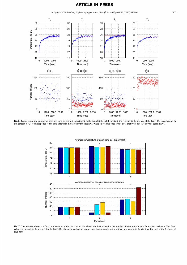
Fig. 7, which will be used to compare the results of all the
experiments, shows the average temperature (top plot) and the
average number of bees (bottom plot) for the last 100 s. The datafor experiment 1 show how an ideal free distribution is achieved.
As we can see, the final temperature reached by all zones is
around 27 3C. In terms of the average number of bees for the last
100 s, we can see that the voltage allocated is around 1.7 V (DC
offset included), which is equivalent to 35 bees per zone.
However, due to the differences between sensors and lamps,
more bees are allocated in the fourth zone (i.e., zone 4 is more
difficult to heat). This result is consistent with the experimental
results shown below.
4.3. Experiment 2: one hive with disturbances, IFD, cross-inhibition,
and site truncation
The second experiment is similar to the first one, but we add
two disturbances to the system. These disturbances are created by
two extra lamps, one placed next to zone 1 and another placed
next to zone 4. We start the experiment at a room temperature of
T a ¼ 20:6 3C. Fig. 5 shows the results. The numbers in the top left
and top right plots represent the disturbance types applied to the
0 1000 2000 300018
20
22
24
26
28
30
T e m p e r a t u r e ,
d e g
C
T1
Time (sec)
0 1000 2000 300018
20
22
24
26
28
30
T2
Time (sec)
0 1000 2000 300018
20
22
24
26
28
30
T3
Time (sec)
0 1000 2000 300018
20
22
24
26
28
30
T4
Time (sec)
0 1000 2000 3000
0
20
40
60
80
100
N u m b e r o f b e e s
x1
Time (sec)
0 1000 2000 3000
0
20
40
60
80
100
x2
Time (sec)
0 1000 2000 3000
0
20
40
60
80
100
x3
Time (sec)
0 1000 2000 3000
0
20
40
60
80
100
x4
Time (sec)
Fig. 3. Temperature and number of bees per zone when there is one hive and no disturbances. The top plots show the temperature in each zone, and the average of the last
100 s (solid constant line). The stems in the bottom plots represent the number of bees that were allocated to each zone.
N. Quijano, K.M. Passino / Engineering Applications of Artificial Intelligence 23 (2010) 845–861854

8/6/2019 Honey Bee Resource Allocation
http://slidepdf.com/reader/full/honey-bee-resource-allocation 11/17
ARTICLE IN PRESS
0 500 1000 1500 2000 2500 3000
0
50
100
150
200
Bf
Time (sec)
0 500 1000 1500 2000 2500 3000
0
1020
30
40
50
60
70
Be
Time (sec)
Fig. 4. Number of employed foragers B f and the average of the last 100 s (top plot). The bottom plot shows the number of explorers Be and the average of the last 100 s.
0 500018
20
22
24
26
28
30
T e m p e r a t u r e ,
d e g C
T1
Time (sec)
0 500018
20
22
24
26
28
30
T2
Time (sec)
0 500018
20
22
24
26
28
30
T3
Time (sec)
0 500018
20
22
24
26
28
30
T4
Time (sec)
0 50000
20
40
60
80
100
120
N u m b e r o f b e e s
x1
Time (sec)
0 50000
20
40
60
80
100
120
x2
Time (sec)
0 50000
20
40
60
80
100
120
x3
Time (sec)
0 50000
20
40
60
80
100
120
x4
Time (sec)
21
33
Fig. 5. Temperature and number of bees per zone for the second experiment. In the top plot the solid constant line represents the average of the last 100 s in each zone. The
numbers 1–3 correspond to the disturbances. The stems in the bottom plot represent the number of bees that were allocated to each zone.
N. Quijano, K.M. Passino / Engineering Applications of Artificial Intelligence 23 (2010) 845–861 855

8/6/2019 Honey Bee Resource Allocation
http://slidepdf.com/reader/full/honey-bee-resource-allocation 12/17
8/6/2019 Honey Bee Resource Allocation
http://slidepdf.com/reader/full/honey-bee-resource-allocation 13/17
ARTICLE IN PRESS
1 2 3
18
20
22
24
26
28
30
Average temperature of each zone per experiment
T e m p e r a t u r e ,
d e g C
1 2 3
0
20
40
60
80
100
120
140 Average number of bees per zone per experiment
Experiment
N u m b e r o f B e e s
Fig. 7. The top plot shows the final temperature, while the bottom plot shows the final value for the number of bees in each zone for each experiment. This final
value corresponds to the average for the last 100 s of data. In each experiment, zone 1 corresponds to the left bar, and zone 4 to the right bar for each of the 3 groups of
four bars.
0 1000 200018
20
22
24
26
28
30
T e m p e r a t u r e ,
d e g C
T1
Time (sec)
0 1000 200018
20
22
24
26
28
30
T2
Time (sec)
0 1000 200018
20
22
24
26
28
30
T3
Time (sec)
0 1000 200018
20
22
24
26
28
30
T4
Time (sec)
0 1000 2000 30000
50
100
150
x1
1(o)
Time (sec)
N u m b e r o f b e e s
0 1000 2000 30000
50
100
150
x2
1(o), x
2
2(x)
Time (sec)
0 1000 2000 30000
50
100
150
x3
1(o), x
3
2(x)
Time (sec)
0 1000 2000 30000
50
100
150
x4
2(x)
Time (sec)
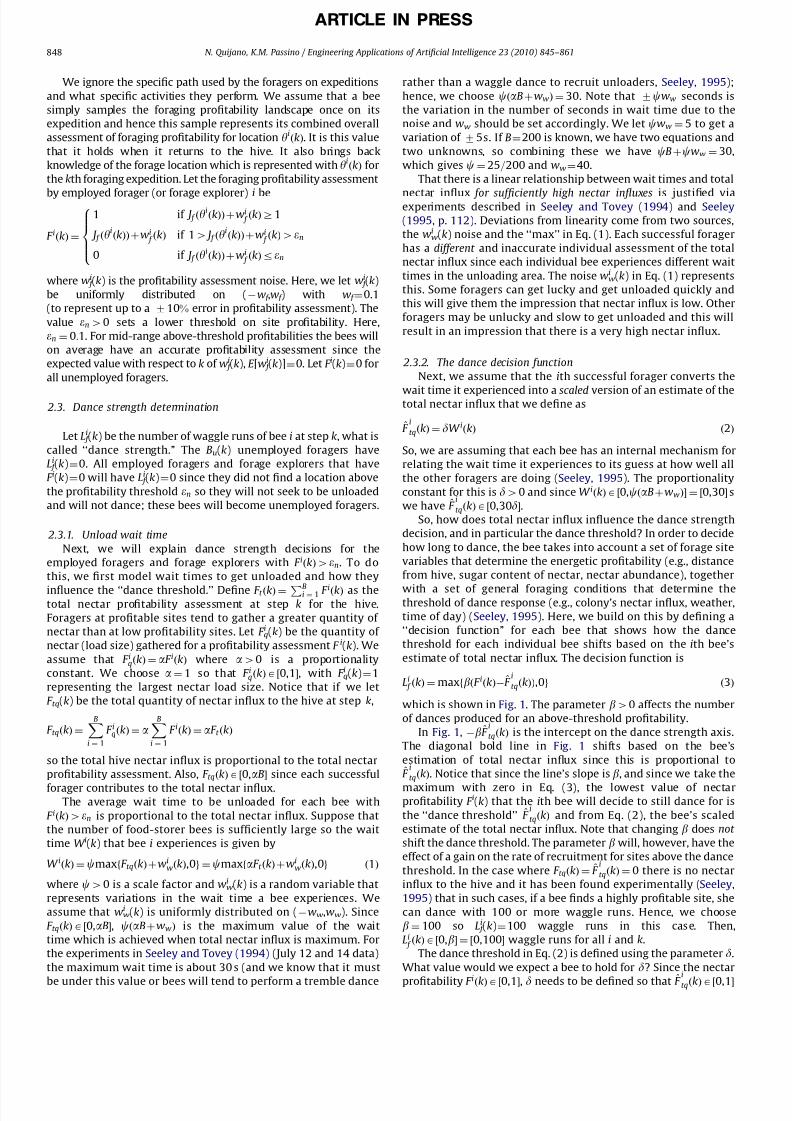
Fig. 6. Temperature and number of bees per zone for the last experiment. In the top plot the solid constant line represents the average of the last 100 s in each zone. In
the bottom plot, ‘‘o’’ corresponds to the bees that were allocated by the first hive, while ‘‘x’’ corresponds to the bees that were allocated by the second hive.
N. Quijano, K.M. Passino / Engineering Applications of Artificial Intelligence 23 (2010) 845–861 857
8/6/2019 Honey Bee Resource Allocation
http://slidepdf.com/reader/full/honey-bee-resource-allocation 14/17
ARTICLE IN PRESS
practically the same number of bees visited sites 1, 2, and 3 (45,
31, 34 visited on average zones 1 through 3, respectively, while 60
bees where allocated to zone 4 due to sensor differences). When
disturbance 1 is applied, more bees start visiting sites 1, 2, and 3,
while the number of bees in zone 4 reduces drastically. The same
thing happens when disturbances 2 and 3 are applied. It is clear
that in any of these cases one or two zones becomes less
profitable (the temperature increases due to the disturbance, and
hence the error decreases), which implies that the hive has toreduce the number of bees recruited to these poorer sites. This is
given in the algorithm by a reduction of the number of dances for
those zones where the error is smaller, which leads to a reduction
in the number of bees that are recruited to these sites.
Experiment 3 shows how another IFD is achieved over all
zones, even though there is not perfect information (see Fig. 7).
As we can see in Fig. 6, the final temperature in all zones is prac-
tically the same (taking into account the sensor differences
accuracy). However, as we mentioned before, hive 2 must use
more of its bees to raise the temperature in zone 4, and that is
why the number of bees allocated by this hive to zones 2 and 3 is
small. This problem can be seen also as having a zone with a
disturbance. In this case, zone 4 needs more energy, which
implies that more bees are allocated by the second hive to it. Thus,
the middle zones are not visited as much by the bees since they
are less profitable. They are also not as profitable as zone 1, and
that is why a smaller amount of bees are allocated to zones 2 and
3 by hive 1 (compared to those that are allocated in zone 1 as it
can be seen in the bottom plot in Fig. 6). However, the total
number of bees (those allocated by hives 1 and 2) leads to prac-
tically the same numbers of bees in zones 2 and 3, and the grid
reaches a maximum uniform temperature.
In all these cases, the temperature grid reached an equilibrium.
If we compare the experimental results with the theoretical
results (Section 3), we can see that the equilibrium point for the
first experiment is similar to what is shown in Theorem 3.2. In
this case, the a j can be seen as the temperature error, because it is
clear that the hive will allocate more bees where the error is
higher. For the last experiment a population level type IFD as in
(19) is achieved, again with a j proportional to the temperature
error. We have proven in Theorem 3.3 that the IFD was the
optimum point, and the experiments illustrate that this equili-
brium was reached for n¼2 hives.
5. Conclusions
In this paper we provided a novel bio-inspired resource
allocation method, developed theory to explain key properties
of the algorithm, and studied an application that illustrates the
validity of the theoretical properties. The application that we have
used is a multizone temperature control grid, where the control
objective is to seek the maximum uniform temperature. InQuijano and Passino (2007) the authors use the same testbed to
show how the replicator dynamics model leads to an ideal free
distribution (IFD). Here, the honey bee social foraging algorithm
gives us similar results, and also helped us to illustrate dynamic
re-allocation, cross-inhibition, and the IFD. We leave as an
important future direction the comparative analysis with the
performance of other methods for the experimental testbed.
Clearly, there are other applications for the social foraging method
for allocation, for instance, in the area of formation control and
task allocation of multiple agents.
The game and optimization theoretic theory that characterizes
properties of the social foraging algorithm is a key contribution of
this paper. One of the most important concepts in this paper is the
IFD concept from theoretical ecology. We have shown that the IFD
is a strict Nash equilibrium for an n-hive game and a one-stable
ESS. In other words, in an n-hive game the IFD is reached
whenever n À1 hives are using it as a strategy and only one hive is
not using it. This hive has to choose the IFD strategy to obtain as
much as the other hives. Since this is only a local concept, we
extend our results to show that the IFD is a global optimum point
for both a single hive and multiple hives. In this case we have
limited our analysis to an optimality perspective. It is our intent to
develop in the future a dynamical model of IFD achievement(e.g., adaptive dynamics such as a replicator dynamics model,
Hofbauer and Sigmund, 1998).
Finally, it is clear that in the implementation we have limited
our system and drawn some analogies that might not seem real
from a biological perspective. For instance, consider the informa-
tion structure of the algorithm (i.e., what characteristics are
present to provide information to the algorithm and between
components of the algorithm). In a honey bee hive, the forage
allocation process does not need a centralized entity that makes
the decisions and allocates bees to each site, i.e., the hive is a
decentralized system (Seeley, 1995). However, if we analyze the
honey bee social foraging algorithm, and more precisely Eqs. (1),
(5) and (6), it is clear that the algorithm is not totally
‘‘individual-based’’ (e.g., Eq. (5) has to know a noisy version of
the total number of waggle runs in order to decide how many
observer bees will become an explorer). It is our intent to consider
in the future a more fully distributed version that faithfully
respects what is known by individuals. Also, other large-scale
optimization problems will be considered to show the applic-
ability of our algorithm. Finally, it is our hope to in the future
conduct a more complete mathematical and experimental
evaluation of the robustness of our distributed dynamical
control system.
Acknowledgements
This research was supported in part by the OSU Office of
Research. We would like to thank Thomas D. Seeley for a numberof fruitful conversations on the biology of honey bee social
foraging. Also, we would like to thank Jorge Finke for checking the
simulation code for the honey bee social foraging algorithm and
for some suggestions on the manuscript.
The authors would like to thank NIST for support for
development of the temperature control experiment. Also, we
would like to thank the OSU office of Research for partial financial
support via an interdisciplinary research grant.
Appendix A. Proofs of theorems
A.1. Proof of Theorem 3.1
We will show that if x ià ¼ ½ xiÃ1 , xiÃ
2 , . . . , xiÃN �
>, where
xià j ¼ B f a j=
PN j ¼ 1 a j for all j¼1,2,y,N , and i ¼1,2,y,n, then a single
hive mutant y ia xià will have a lower fitness for the moment,
when yiAD xÀ@D x (i.e., strictly inside the simplex). This is
equivalent to show that Eq. (7) is satisfied for all i ¼1,2,y,n.
But, it can also be seen as a constrained optimization problem of
the form
maximize f i ¼XN
j ¼ 1
xi j
a jPnk ¼ 1 xk
j
subject toXN
j ¼ 1
xi j ¼ B f , i ¼ 1,2, . . . ,n
x
i
j4
0,
j ¼ 1,
2, . . . ,
N
N. Quijano, K.M. Passino / Engineering Applications of Artificial Intelligence 23 (2010) 845–861858

8/6/2019 Honey Bee Resource Allocation
http://slidepdf.com/reader/full/honey-bee-resource-allocation 15/17
ARTICLE IN PRESS
xk j ¼
B f a jPN m ¼ 1 am
, ka i, k ¼ 1,2, . . . ,n ð21Þ
This is a nonlinear optimization problem that we will solve using
Lagrange multiplier theory (e.g., Bertsekas, 1995).
First, since xi j40 the constraint is inactive, so it can be ignored.
Second, replace in Eq. (10) the constraint xk j ¼ B f a j=
PN m ¼ 1 am, for
all ka i to get
f i ¼XN
j ¼ 1
xi j
a j
xi j þf j
where
f j ¼Xn
k ¼ 1,ka i
B f a jPN m ¼ 1 am
¼ ðnÀ1ÞB f a jPN
m ¼ 1 am
ð22Þ
The problem in Eq. (21) becomes
maximize f i
subject to XN
j ¼ 1
xi j ¼ B f , i ¼ 1,2, . . . ,n
Now, we define the vector x ¼ ½ xi1, xi
2, . . . , xiN �
> which constitutes
the points for which we want to find an extremizer point.
Let hð xÞ ¼PN
j ¼ 1 xi jÀB f . The gradient of f i with respect to x is
equal to
r f ið xÞ ¼@ f i
@ xi1
,
@ f i
@ xi2
, . . . ,
@ f i
@ xiN
" #>
r f ið xÞ ¼a1f1
ð xi1 þf1Þ2
,
a2f2
ð xi2 þf2Þ2
, . . . ,
aN fN
ð xiN þfN Þ
2
" #>
Also, @h=@ xi j ¼ 1 for all j¼1,2,y,N . Let là be the
Lagrange multiplier for this constrained optimizationproblem. Then, we have to solve the following set of equations
for xià j 40:
a1f1
ð xiÃ1 þf1Þ2
þlü 0
^
aN fN
ð xiÃN þfN Þ
2þl
ü 0
xiÃ1 þ xiÃ
2 þ Á Á Á þ xiÃN ¼ B f
For any i, j ¼ 1,2, . . . ,N we have from the previous equations that
aifi
ð xiÃ
iþf
iÞ2
¼a jf j
ð xià j
þf j
Þ2
Using Eq. (22),
a2
i
ð xiÃ
i
PN m ¼ 1 am þB f ai
ðnÀ1ÞÞ2¼
a2
j
ð xiÃ
j
PN m ¼ 1 am þB f a j
ðnÀ1ÞÞ2
Since a j40 and xi j40, j¼1,2,y,N , i ¼1,2,y,n, and n41,
ai
xiÃ
j
XN
m ¼ 1
am þB f a jðnÀ1Þ
!¼ a
jxiÃ
i
XN
m ¼ 1
am þB f aiðnÀ1Þ
!
Simplifying, we get that for all i, j ¼ 1,2, . . . ,N ,
ai
xiÃ
j
¼ a j
xiÃ
i
After some algebraic manipulations, this implies that for all
i ¼ 1,2, . . . ,N ,
xiÃ
i¼
B f aiPN m ¼ 1 am
ð23Þ
In order to see that xiÃ
idefined in Eq. (23) is a local maximum
we need to prove the second order sufficiency condition. For that,
we need to analyze the Hessian of f j (because the Hessian of h( x) is
0). In this case,
r 2 f jð xÞ ¼
À2a1f1
ð xi1 þf1Þ3
0 . . . 0
0À2a2f2
ð xi2 þf2Þ3
. . . 0
^ ^ & ^
0 0 . . .À2aN fN
ð xiN þfN Þ
3
2666666666664
3777777777775
It is clear that the Hessian of f i( x) for x jin, j¼1,2,y,N , i ¼1,2,y,n,
in Eq. (23) is negative definite since a j40, x j40, n41 and f j40,
j¼1,2,y,N . Therefore we can conclude that the extremizer points
defined in Eq. (23) are global maximizers (because it is clear that
the cost function is convex on the simplex D x). Hence, x jin
definedby Eq. (23) (which is equivalent to Eq. (13)) is a strict Nash
equilibrium. Also, since it is a strict Nash equilibrium, Eq. (8)
holds. Therefore, the IFD is a one-stable ESS for the finite
population in a game against the field.
A.2. Proof of Theorem 3.2
As in the case for the proof of Theorem 3.1, x j40 is an inactive
constraint so it can be ignored. Let hð xÞ ¼PN
j ¼ 1 x jÀB f . For this
case, we will have that the gradient of h( x) is equal to
r hð xÞ ¼ ½1,1, . . . ,1�>
and the gradient for J ( x) is given by
r J ð xÞ ¼2 x1
B f a1,
2 x2
B f a2, . . . ,
2 xN
B f aN
>
Let lÃ
be the Lagrange multiplier for this constrained optimization
problem. Then, we have to solve the following set of equations for
xà j 40:
2 xÃ1
B f a1þlÃ
¼ 0
^
2 xÃN
B f aN þl
Ã
¼ 0
xÃ1 þ xÃ
2 þ Á Á Á þ xÃN ¼ B f
As in the proof of Theorem 3.1 this implies that
ak xÃ
j ¼ a j xÃk
for all j,k ¼ 1,2, y, N , which implies that
xà j ¼
B f a jPN j ¼ 1 a j
ð24Þ
In order to see that x jn defined in Eq. (24) is a local minimum we
need to prove the second order sufficiency condition. For that, we
need to analyze the Hessian of J (because the Hessian of h( x) is 0).
N. Quijano, K.M. Passino / Engineering Applications of Artificial Intelligence 23 (2010) 845–861 859
8/6/2019 Honey Bee Resource Allocation
http://slidepdf.com/reader/full/honey-bee-resource-allocation 16/17
ARTICLE IN PRESS
In this case,
r 2 J ð xÃÞ ¼
2
B f a10 . . . 0
02
B f a2. . . 0
^ ^ & ^
0 0 . . .2
B f
aN
266666666664
377777777775
Since, B f 40 and a j40, j¼1,2,y,N , r 2 J ð xÃÞ is positive definite,
which implies by the second-order sufficient condition that xn j in
Eq. (24) is a local minimizer. However, we know that the cost
function J is defined over a simplex D x, which is nonempty,
convex, and a closed subset of RN . Using this fact, and since the
Hessian of J ( xn) is positive definite, we can conclude that the local
minimum in Eq. (24) is also global (Bertsekas, 1995).
A.3. Proof of Theorem 3.3
From an optimization point of view, the problem that we want
to solve is the same as
maximize f i
subject toXN
j ¼ 1
x ji ¼ B f , i ¼ 1,2, . . . ,n
xi j40, j ¼ 1,2, . . . ,N
xi j ¼
nB f a jPN j ¼ 1 a j
ÀXn
k ¼ 1,ka i
xk j , ia i ð25Þ
Let hð xÞ ¼PN
j ¼ 1 xi jÀB f , and since xi
j40 that constraint is
inactive, so it can be ignored. Using Lagrange multipliers, we
need to find first the gradient of the cost function and the gradient
of the constraint. In this case, we have
r f i ¼@ f i
@ xi1
,
@ f i
@ xi2
, . . . ,
@ f i
@ xiN
" #>
where
@ f i
@ xi j
¼a j
Pnk ¼ 1,ka i xk
j
ð xi j þ
Pnk ¼ 1,ka i xk
j Þ2
The gradient of h( x) is r hð xÞ ¼ ½1,1, . . . ,1�>. Therefore, we have to
solve the following set of equations for xià j 40:
a1
Pnk ¼ 1,ka i xkÃ
1
ð xiÃ1 þ
Pnk ¼ 1,ka i xkÃ
1 Þ2þlÃ
¼ 0
^
aN
Pnk ¼ 1,ka i xkÃ
N
ð xiÃN þ
Pnk ¼ 1,ka i xkÃ
N Þ2þl
ü 0
xiÃ1 þ xiÃ
2 þ . . . xiÃN ¼ B f
Then, for any i, j ¼ 1,2, . . . ,N ,
ai
Pnk ¼ 1,ka i xkÃ
i
ð xiÃi
þPn
k ¼ 1,ka i xkÃ
iÞ2
¼a
j
Pnk ¼ 1,ka i xkÃ
j
ð xiÃ
jþPn
k ¼ 1,ka i xkÃ
jÞ2
Replacing the constraint in Eq. (25),
ai
nPaiPN
j ¼ 1 a j
À xiÃ
i !n2B2
f a2
j
ðPN
j ¼ 1 a jÞ
2¼ a
j
nPa j
PN
j ¼ 1 a j
À xiÃ
j !n2B2
f a2
i
ðPN
j ¼ 1 a jÞ
2
which implies that
a j xiÃ
i¼ a
i xiÃ
j
xiÃi
¼a
iB f PN
j ¼ 1 a j
ð26Þ
The point in Eq. (26) is an extremizer for the optimization
problem defined in (25). Now, let us prove that (26) is indeed a
global maximizer for this problem. For that, we need to analyzeonly the Hessian of our cost function because r 2hð xÞ ¼ 0. That is,
r 2 f ið xÃÞ ¼
À2a1
Pnk ¼ 1,ka i xkÃ
1
ð xi1 þ
Pnk ¼ 1,ka i xkÃ
1 Þ30
^ & ^
0À2aN
Pnk ¼ 1,ka i xkÃ
N
ð xiN þ
Pnk ¼ 1,ka i xkÃ
N Þ3
266666664
377777775
Clearly, since a j40, B f 40, xià j 40,
Pnk ¼ 1,ka i xkÃ
1 40, and n41, the
Hessian is negative definite. Therefore we can conclude that
the extremizer points defined in Eq. (26) are global maxi-
mizers (because it is clear that the cost function is convex on
the simplex D x).
Replacing the optimum point, we can notice that theconstraint becomes xi
j ¼ nB f a j=PN
j ¼ 1 a jÀPn
k ¼ 1,ka ixk
j that is
equivalent to Eq. (19).
References
Alaeddine, M., Doumanidis, C.C., 2004a. Distributed parameter thermal controll-ability: a numerical method for solving the inverse heat conduction problem.International Journal for Numerical Methods in Engineering 59 (7), 945–961.
Alaeddine, M., Doumanidis, C.C., 2004b. Distributed parameter thermal systemcontrol and observation by Green–Galerkin methods. International Journal forNumerical Methods in Engineering 61 (11), 1921–1937.
Anderson, C., 2001. The adaptive value of inactive foragers and the scout-recruitsystem in honey bee (Apis mellifera) colonies. Behavioral Ecology 12 (1), 111.
Bas-ar, T., Olsder, G.J., 1999. Dynamic Noncooperative Game Theory. SIAM,Philadelphia, PA.
Bartholdi, J., Seeley, T.D., Tovey, C., VandeVate, J., 1993. The pattern and
effectiveness of forager allocation among flower patches by honey beecolonies. Journal of Theoretical Biology 160, 23–40.
Bertsekas, D.P., 1995. Nonlinear Programming. Athena Scientific Press, Belmont,MA.
Bonabeau, E., Dorigo, M., Theraulaz, G., 1999. Swarm Intelligence: From Natural toArtificial Systems. Oxford University Press, New York, NY.
Camazine, S., Sneyd, J., 1991. A model of collective nectar source selection byhoney bees: self-organization through simple rules. Journal of TheoreticalBiology 149, 547–571.
Chong, C., Sivakumar, A., Low, M., Gay, K., 2006. A bee colony optimizationalgorithm to job shop scheduling. In: Proceedings of the 37th Conference onWinter Simulation N/A, pp. 1954–1961.
Cox, M., Myerscough, M., 2003. A flexible model of foraging by a honey bee colony:the effects of individual behavior on foraging success. Journal of TheoreticalBiology 223, 179–197.
Crawford, V.P., 1990. Nash equilibrium and evolutionary stability in large- andfinite-population ‘‘Playing the Field Models’’. Journal of Theoretical Biology145, 83–94.
de Vries, H., Biesmeijer, J.C., 1998. Modeling collective foraging by means of individual behavior rules in honey-bees. Behavioral Ecology and Sociobiology44, 109–124.
de Vries, H., Biesmeijer, J.C., 2002. Self-organization in collective honeybeeforaging: emergence of symmetry breaking, cross inhibition, and equalharvest-rate distribution. Behavioral Ecology and Sociobiology 51, 557–569.
Demetriou, M.A., Paskaleva, A., Vayena, O., Doumanidis, H., 2003. Scanningactuator guidance scheme in a 1-d thermal manufacturing process. IEEETransactions on Control Systems Technology 11 (5), 757–764.
Dorigo, M., Blum, C., 2005. Ant colony optimization theory: a survey. TheoreticalComputer Science 344 (2–3), 243–278.
Dorigo, M., Gambardella, L., Middendorf, M., Stutzle, T., 2002. Guest editorial:special section on ant colony optimization. IEEE Transactions on EvolutionaryComputation 6 (4), 317–319.
Dorigo, M., Maniezzo, V., 1996. The ant system: optimization by a colony of cooperating agents. IEEE Transactions on Systems, Man, and Cybernetics, PartB 26 (1), 29–41.
Dorigo, M., Maniezzo, V., Colorni, A., 1996. Ant system: optimization by a colonyof cooperating agents. IEEE Transactions on Systems, Man, and Cybernetics,
Part B 26 (1), 29–41.
N. Quijano, K.M. Passino / Engineering Applications of Artificial Intelligence 23 (2010) 845–861860
8/6/2019 Honey Bee Resource Allocation
http://slidepdf.com/reader/full/honey-bee-resource-allocation 17/17
ARTICLE IN PRESS
Dorigo, M., Stutzle, T., 2004. Ant Colony Optimization. MIT Press, Cambridge, MA.Dukas, R., Edelstein-Keshet, L., 1998. The spatial distribution of colonial food
provisioners. Journal of Theoretical Biology 190, 121–134.Emami-Naeini, A., Ebert, J., de Roover, D., Kosut, R., Dettori, M., Porter, L.M.L.,
Ghosal, S., 2003. Modeling and control of distributed thermal systems. IEEETransactions on Control Systems Technology 11 (5), 668–683.
Fretwell, S.D., Lucas, H.L., 1970. On territorial behavior and other factorsinfluencing habitat distribution in birds. Acta Biotheoretica 19, 16–36.
Giraldeau, L.A., Caraco, T., 2000. Social Foraging Theory. Princeton University Press,Princeton, NJ.
Han, P., Huang, Y., Jia, Z., Wang, D., Li, Y., 2005. Mixed H2/HN optimal PID control
for superheated steam temperature system based on PSO optimization.Proceedings of 2005 International Conference on Machine Learning andCybernetics, 2005, vol. 2; 2005, pp. 960–964.
Hofbauer, J., Sigmund, K., 1998. Evolutionary Games and Population Dynamics.Cambridge University Press, Cambridge, UK.
Ibaraki, T., Katoh, N., 1988. Resource Allocation Problems: Algorithmic Approaches.The MIT Press, Cambridge, MA.
Jones, P.D., Duncan, S.R., Rayment, T., Grant, P.S., 2003. Control of temperatureprofile for a spray deposition process. IEEE Transactions on Control SystemsTechnology 11 (5), 656–667.
Juang, C.-F., Hsu, C.-H., 2005. Temperature control by chip-implemented adaptiverecurrent fuzzy controller designed by evolutionary algorithm. IEEE Transac-tions on Circuits and Systems I: Regular Papers 52 (11), 2376–2384.
Karaboga, D., 2005. An idea based on honey bee swarm for numerical optimization.Technical Report-tr06, Erciyes University, Engineering Faculty, ComputerEngineering Department.
Kennedy, J., Eberhart, R., 1995. Particle swarm optimization. Proceedings IEEEInternational Conference on Neural Networks, vol. 4; 1995, pp. 1942–1948.
Kennedy, J., Eberhart, R., 2001. Swarm Intelligence. Morgan Kaufmann PublishersInc., San Francisco, CA, USA, p. 512.Maynard Smith, J., 1982. Evolution and the Theory of Games. Cambridge
University Press, Cambridge, UK.Maynard Smith, J., 1988. Can a mixed strategy be stable in a finite population?
Journal of Theoretical Biology 130 247–251.Maynard Smith, J., Price, G.R., 1973. The logic of animal conflict. Nature 246,
15–18.Mitchell, M., 1996. An Introduction to Genetic Algorithms. MIT Press, Cambridge,
MA.Nakrani, S., Tovey, C., 2003. On honey bees and dynamic allocation in an internet
server colony. In: Proceedings of 2nd International Workshop on theMathematics and Algorithms of Social Insects.
Neill, D.B., 2004. Evolutionary stability for large populations. Journal of TheoreticalBiology 227, 397–401.
Pankiw, T., 2005. The honey bee foraging behavior syndrome: quantifying theresponse threshold model of division of labor. In: Swarm IntelligenceSymposium, 2005. SIS 2005. Proceedings 2005. IEEE N/A, pp. 1–6.
Parker, G.A., 1978. Searching for mates. In: Krebs, J.R., Davies, N.B. (Eds.),
Behavioural Ecology: An Evolutionary Approach, pp. 214–244.Parker, G.A., Sutherland, W.J., 1986. Ideal free distribution when individuals differ
in competitive ability: phenotype-limited ideal free models. Animal Behaviour34, 1222–1242.
Passino, K.M., 2005. Biomimicry for Optimization, Control, and Automation.Springer-Verlag, London.
Passino, K.M., Seeley, T.D., 2006. Modeling and analysis of nest-site selection byhoney bee swarms: the speed and accuracy trade-off. Behavioral Ecology andSociobiology 59 (3), 427–442.
Pham, D., Ghanbarzadeh, A., Ko, E., Otri, S., Rahim, S., Zaidi, M., 2006. The beesalgorithm, a novel tool for complex optimisation problems. In: Proceedings of the 2nd International Virtual Conference on Intelligent Production Machinesand Systems (IPROMS 2006) N/A, N/A.
Poli, R., 2007. An analysis of publications on particle swarm optimizationapplications. Technical Report CSM-469, Department of Computer Science,University of Essex.
Poli, R., Kennedy, J., Blackwell, T., 2007. Particle swarm optimization. SwarmIntelligence 1, 33–57.
Quijano, N., Gil, A.E., Passino, K.M., 2005. Experiments for dynamic resourceallocation, scheduling, and control. IEEE Control Systems Magazine 25,63–79.
Quijano, N., Passino, K.M., 2007. The ideal free distribution: theory and engineeringapplication. IEEE Transactions on Systems, Man, and Cybernetics—Part B 37(1), 154–165.
Reimann, M., Doerner, K., Hartl, R., 2004. D-Ants: savings based ants divide andconquer the vehicle routing problem. Computers and Operations Research 31(4), 563–591.
Riley, J.G., 1979. Evolutionary equilibrium strategies. Journal of Theoretical Biology76, 109–123.
Ross, P.E., 2004. Beat the heat. IEEE Spectrum Magazine 41 (5), 38–43.Schaffer, M.E., 1988. Evolutionary stable strategies for a finite population
and a variable contest size. Journal of Theoretical Biology 132,469–478.
Schaper, C.D., El-Awady, K., Tay, A., 1999a. Spatially-programmable temperaturecontrol and measurement for chemically amplified photoresist processing.SPIE Conference on Process, Equipment, and Materials Control in IntegratedCircuit Manufacturing, vol. 3882; 1999, pp. 74–79.
Schaper, C.D., Kailath, T., Lee, Y.J., 1999b. Decentralized control of wafertemperature for multizone rapid thermal processing systems. IEEE Transac-tions on Semiconductor Manufacturing 12 (2), 193–199.
Schoonderwoerd, R., Holland, O.E., Bruten, J.L., Rothkrantz, L.J.M., 1996. Ant-basedload balancing in telecommunications networks. Adaptive Behavior 5 (2),169–207.
Seeley, T., Camazine, S., Sneyd, J., 1991. Collective decision-making in honey bees:how colonies choose among nectar sources. Behavioral Ecology and Socio-
biology 28, 277–290.Seeley, T., Towne, W., 1992. Tactics of dance choice in honeybees:Do foragers compare dances? Behavioral Ecology and Sociobiology 3059–69.
Seeley, T., Visscher, P., 1988. Assessing the benefits of cooperation in honey beeforaging: search costs, forage quality, and competitive ability. BehavioralEcology and Sociobiology 22, 229–237.
Seeley, T.D., 1983. Division of labor between scouts and recruits in honeybeeforaging. Behavioral Ecology and Sociobiology 12, 253–259.
Seeley, T.D., 1994. Honey bee foragers as sensory units of their colonies. BehavioralEcology and Sociobiology 34, 51–62.
Seeley, T.D., 1995. The Wisdom of the Hive. Harvard University Press, Cambridge,MA.
Seeley, T.D., Tovey, C., 1994. Why search time to find a food-storer bee accuratelyindicates the relative rates of nectar collecting and nectar processing in honeybee colonies. Animal Behaviour 47, 311–316.
Stephens, D., Krebs, J., 1986. Foraging Theory. Princeton University Press,Princeton, NJ.
Sumpter, D., Pratt, S., 2003. A modelling framework for understanding social insect
foraging. Behavioral Ecology and Sociobiology 53, 131–144.Teodorovic, D., Dell’orco, M., 2005. Bee colony optimization—a cooperative
learning approach to complex transportation problems. Advanced OR and AIMethods in Transportation N/A, 51–60.
Teodorovic, D., Dell’orco, M., 2008. Mitigating traffic congestion: solving the ride-matching problem by bee colony optimization. Transportation Planning andTechnology 31 (2), 135–152.
Walker, R., 2004. Honeybee search strategies: adaptive exploration of aninformation ecosystem. Evolutionary Computation, 19–23 June 2004.CEC2004. Congress on 1, vol. 1, pp. 1209–1216.
Wedde, H., Farooq, M., 2005. The wisdom of the hive applied to mobile ad-hocnetworks. In: Swarm Intelligence Symposium, 2005. SIS 2005. Proceedings2005 IEEE N/A, pp. 341–348.
Zaheer-uddin, M., Patel, R.V., Al-Assadi, S.A.K., 1993. Design of decentralized robustcontrollers for multizone space heating systems. IEEE Transactions on ControlSystems Technology 1 (4), 246–261.
N. Quijano, K.M. Passino / Engineering Applications of Artificial Intelligence 23 (2010) 845–861 861


![[PPT]Honey Bee Anatomy & Biology - Illinois State Universitywenning/HIBA/Workshop PPTs/Honey Bee... · Web viewHoney Bee Apis mellifera Anatomy & Biology Honey Bee External Anatomy](https://static.fdocuments.net/doc/165x107/5b0a09fe7f8b9aba628b8dcf/ppthoney-bee-anatomy-biology-illinois-state-wenninghibaworkshop-pptshoney.jpg)