Homework 7 - Solution - Purdue Universityovitek/STAT526-Spring11_files/pdfs/hw7... · Data were...

STAT 526 - Spring 2011 Olga VitekHomework 7 - Solution

Each part of the problems 5 points

1. [Methods qualifying exam, August 2009: use paper and pencil.] Data were collected to study a typeof damage caused by waves to the forward section of certain cargo-carrying vessels. The values of thefollowing variables were recorded:

type: ship type (coded as A to E);

year: year of construction (1960, 1965, 1970, 1975);

period: period of operation (1960-74, 75-79);

service: aggregate months of service

incidents: number of damage incidents

Call:

glm(formula = incidents ~ offset(log(service)) + type + year + period, family=poisson, data=wdships)

Deviance Residuals:

Min 1Q Median 3Q Max

-1.6768 -0.8293 -0.4370 0.5058 2.7912

Coefficients:

Estimate Std. Error z value Pr(>|z|)

(Intercept) -6.40590 0.21744 -29.460 < 2e-16 ***

typeB -0.54334 0.17759 -3.060 0.00222 **

typeC -0.68740 0.32904 -2.089 0.03670 *

typeD -0.07596 0.29058 -0.261 0.79377

typeE 0.32558 0.23588 1.380 0.16750

year65 0.69714 0.14964 4.659 3.18e-06 ***

year70 0.81843 0.16977 4.821 1.43e-06 ***

year75 0.45343 0.23317 1.945 0.05182 .

period75 0.38447 0.11827 3.251 0.00115 **

(Dispersion parameter for poisson family taken to be 1)

Null deviance: 146.328 on 33 degrees of freedom

Residual deviance: 38.695 on 25 degrees of freedom

AIC: 154.56

(a) Describe the model used in the above analysis (in terms of the distribution for the responsevariable, and the relation of independent variable to the response).

Answer:

The distribution for the response is

Yiind∼ Poisson(λi)

logλi = log(Servicei) +

5∑j=2

βtijtypeij +

4∑k=2

βyikyearik + βp

i2periodi2

1

where parameter for baseline (βtAtypeA, βy

60year60, βp60−74period60−74)

(b) Give the best reason to use offset(log(service)) in the above data analysis.

Answer:

Service measures the aggregate number of months each ship has been in service. This is a measureof the amount of exposure each ship has had to wave damage and hence represents a differentinterval in time for each response (the number of damage incidents). It is accounted for as anoffset in the Poisson regression context.

(c) Does the model fit the data well? Please explain.

Answer:

H0 : logλi = log(Servicei) +X ′β

Ha : logλi 6= log(Servicei) +X ′β

residual deviance= 38.695 > χ225,0.95 = 37.65 Therefore, reject H0 and we conclude that the model

does not fit well.

(d) Should we consider allowing the dispersion parameter to vary? Please explain.

Answer:

φ = 38.69525 = 1.5478 > 1 So, the dispersion parameter should be allowed to vary.

(e) We define year60 <- (year==1960), and rerun the above model with year60 replacing year.The residual deviance is reported as 42.329. Please construct a hypothesis test to state which ofthese two models is better.

Answer:

H0 : new model with ”year60”

Ha : stated model with ”year”

test statistic= 42.329 − 38.693 = 3.634 < χ22,0.95 = 5.99 Therefore, fail to reject H0 and we

conclude that replacing ”year” with ”year60” leads to a better-fitting model.

2. [Methods qualifying exam, January 2007: use paper and pencil.]

The following table contains the counts of leukemia in five counties of California from 1996 to 2000 aswell as the county population in 2000.

2

County Count (ni) Population (xi)Marin 22 247289

Contra Costa 146 948816Alameda 226 1443741

San Francisco 47 776733San Mateo 52 70716

Assume the count Ni with observed value ni follows a Poisson distribution with parameter λi timesthe county population xi, i = 1, . . . , 5. Derive the Pearson and deviance goodness-of-fit tests for thenull hypothesis that the λi are all the same.

Answer:

Here we assume ni ∼ Poisson(θxi). Then, the MLE of θ is

θ =

∑5i=1 ni∑5i=1 xi

= 0.0001414

Thus, the predicted values of ni(ni) are 34.96, 134.13, 204.10, 109.81, 10.00. The Pearson χ2 statisticis

X2 =

5∑i=1

(ni − ni)2

ni= 220.6 > χ2

4,o.95 = 9.49

Therefore reject H0 and we conclude that at least one county has a different λi from the others.

and the deviance goodness of fit is

G2 = 2

5∑i=1

nilognini

= 142.14

Therefore, reject H0 and we have the same conclusion.

3. [Methods qualifying exam, January 2005: use paper and pencil.] During nesting, each female horseshoecrab has a single male crab in the nest but other males reside nearby. These other males are known assatellite crabs. A study was done to investigate whether the size of the female influences the numberof satellite crabs.

The investigators measured each females carapace width and grouped them by 8 width intervals (themidpoints of these intervals are given in the table). The total number of female crabs is given as casesand the total number of satellite crabs is given by satell. The sample mean and variance within eachinterval is also given.

Width Cases Satell Mean Variance22.69 14 14 1.00 2.7723.84 14 20 1.43 8.8824.77 28 67 2.39 6.5425.84 39 105 2.69 11.3826.79 22 63 2.86 6.8827.74 24 93 3.87 8.8128.67 18 71 3.94 16.8830.41 14 72 5.14 8.29

3

A log-linear model was fit to the data as follows:

> g <- glm(satell=width+offset(log(cases)), family=poisson)

> summary(g)

with output

Coefficients:

Estimate Std. Error t-value

Intercept -3.5354702 0.57602076 -6.137748

width 0.1727192 0.02123161 8.135004

The null deviance is 72.37717 on 7 degrees of freedom. The residual deviance is 6.516796 on 6 degreesof freedom.

(a) Can you tell if this model fits the data?

Answer:

Yes, the model fits the data since residual deviance is 6.51. Based on χ26 distribution, it is small

enough.

(b) Explain why an offset of this form was used in this model.

Answer:

The goal of the study is to find the relationship between the number of satellites and the widthof the female crab. However the study measured locations where there were several female crabs,and the difference in the number of satellites per location can be due to the difference in thenumber of females. Therefore we add an offset to account for the difference in the number offemales.

(c) Suppose the model satell=width was fit to the ungrouped data (i.e. without an offset). Fromthe information given, state a problem that might arise.

Answer:

This model considers the number of cases instead of the ratio as the response variable. It will givea large predicted value for number of satell of crabs with a particular measurement of width.Result can not be explained according to the size influences the number of satellite crabs.

4. The dataset arrests.txt on the course website reports the number of individuals stopped duringpolice checks in 75 precincts in New York city.

• The units i are precincts and ethnic groups (i = 1, . . . , n = 3× 75).

• The outcome of interest is stops, i.e. the number of stops of members of that ethnic group andprecincts

• past.arrests is the number of past arrests of people from that ethnic group and precinct in theprevious year

• precinct is the id of the precinct

4

• eth is the id of the ethnic group (1=african americans, 2=hispanic, 3=white)

• crime is the indicator of the type of the crime

One would like to know whether there is a difference in the average number of police stops by precinct

and by ethnicity, while treating past.arrests as a measure of “exposure”.

(a) Specify the model that is appropriate for this problem in mathematical notation, and state theassumption. Obtain the model fit. (Hint: use offset= option in glm).

Answer:The response of interest is measured in counts. Therefore an appropriate model is based onPoisson distribution with an offset:

log[E(y)] = log(λi) = log(µiθi) = log(µi) + log(θi)

= log(past.arrestsi) + β0 +

3∑j=2

βeijethnicityij +

75∑j=2

βpikprecinctik

The assumptions include

i. Yi ∼ Poisson(λi), where λi = µiθi.

ii. µi: the exposure, which is past.arrests in this case. It is multiplicative.

iii. θi: the rate, following Poisson regression model.

iv. Observations are independent of each other.

v. At each level, E(Yi) = V ar(Yi).

And the model fit is below,

R code and output

mfull <- glm(formula = stops ~ factor(eth) + factor(precinct),

family=poisson, data=stop, offset=log(past.arrests))

summary(mfull)

Coefficients:


(Intercept) -1.378863 0.051019 -27.026 < 2e-16 ***

factor(eth)2 0.010183 0.006802 1.497 0.134377

factor(eth)3 -0.419023 0.009435 -44.412 < 2e-16 ***

factor(precinct)2 -0.149049 0.074030 -2.013 0.044078 *

factor(precinct)3 0.559956 0.056758 9.866 < 2e-16 ***


...



---

Signif. codes: 0 *** 0.001 ** 0.01 * 0.05 . 0.1 1


5

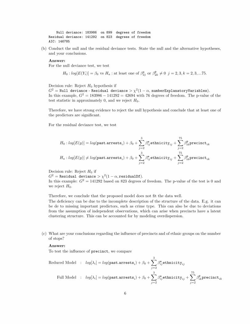
Null deviance: 183986 on 899 degrees of freedom

Residual deviance: 141292 on 823 degrees of freedom

AIC: 146785

(b) Conduct the null and the residual deviance tests. State the null and the alternative hypotheses,and your conclusions.

Answer:For the null deviance test, we test

H0 : log[E(Yi)] = β0 vs Ha : at least one of βe2j or βp2k 6= 0 j = 2, 3, k = 2, 3, ...75.

Decision rule: Reject H0 hypothesis ifG2 = Null deviance - Residual deviance > χ2(1− α, numberExplanatoryVariables).In this example, G2 = 183986 − 141292 = 42694 with 76 degrees of freedom. The p-value of thetest statistic in approximately 0, and we reject H0.

Therefore, we have strong evidence to reject the null hypothesis and conclude that at least one ofthe predictors are significant.

For the residual deviance test, we test

H0 : log[E(y)] = log(past.arrestsi) + β0 +

3∑j=2

βeijethnicityij +

75∑j=2

βpikprecinctik

Ha : log[E(y)] 6= log(past.arrestsi) + β0 +

3∑j=2

βeijethnicityij +

75∑j=2

βpikprecinctik

Decision rule: Reject H0 ifG2 = Residual deviance > χ2(1− α, residualDf).In this example: G2 = 141292 based on 823 degrees of freedom. The p-value of the test is 0 andwe reject H0.

Therefore, we conclude that the proposed model does not fit the data well.

The deficiency can be due to the incomplete description of the structure of the data. E.g. it canbe de to missing important predictors, such as crime type. This can also be due to deviationsfrom the assumption of independent observations, which can arise when precincts have a latentclustering structure. This can be accounted for by modeling overdispersion.

(c) What are your conclusions regarding the influence of precincts and of ethnic groups on the numberof stops?

Answer:

To test the influence of precinct, we compare

Reduced Model : log[λi] = log(past.arrestsi) + β0 +

3∑j=2

βeijethnicityij

Full Model : log[λi] = log(past.arrestsi) + β0 +

3∑j=2

βeijethnicityij +

75∑j=2

βpikprecinctik

6

The decision rule is: Reject H0 hypothesis if

G2 = ResidualDeviance(Reduced)− ResidualDeviance(Full) > χ2(1− α, p− q)

In this example: G2 = 42011, and the p-value based on the χ2 distribution, with 74 degrees offreedom is 0 < 0.05.

Therefore, we reject the null hypothesis and conclude that at the precint a significant predictorof the number of police stops.

To test the influence of ethnicity,

Reduced Model : log[λi] = log(past.arrestsi) + β0 +

75∑j=2

βpikprecinctik

Full Model : log[λi] = log(past.arrestsi) + β0 +

3∑j=2

βeijethnicityij +

75∑j=2

βpikprecinctik

The decision rule is: Reject H0 hypothesis if

G2 = ResidualDeviance(Reduced)− ResidualDeviance(Full) > χ2(1− α, p− q).

In this example: G2 = 2469.4 and P-value based on the χ2 distribution, with degree of freedomof 2 is 0 < 0.05.

Therefore, we reject the null hypothesis and conclude that at the ethnicity is a significant predictorof the number of police stops.

R code and output

## without precint

>influ.prec <- glm(stops ~ factor(eth), family=poisson, data = stop,

offset=log(past.arrests))

>anova(influ.prec, mfull)

Model 1: stops ~ factor(eth)

Model 2: stops ~ factor(eth) + factor(precinct)

Resid. Df Resid. Dev Df Deviance

1 897 183303

2 823 141292 74 42011

## without ethnicity

>influ.eth <- glm(stops ~ factor(precinct), family=poisson, data = stop,

offset=log(past.arrests))

>anova(influ.eth, mfull)

Model 1: stops ~ factor(precinct)

Model 2: stops ~ factor(eth) + factor(precinct)

Resid. Df Resid. Dev Df Deviance

1 825 143762

2 823 141292 2 2469.4

(d) For each precinct and ethnicity, the dataset contains separate entries for crime type. Since crimetype is not used as a predictor, these entries are viewed as independent replicates. Will there be

7

a change in (i) the values of null and residual deviance, (ii) the estimates of the parameters, and(iii) comparisons between nested models if we combine all the entries from a same precinct andethnicity (i.e. add the number of stops and past arrests across all the crime types)? Explain thereasons for your answers, and show numeric output to support your conclusions.

Answer:

i. null and residual deviance are different.before combining, (a) after combining, (d)

null deviance 183986 46120.9df 899 224residual deviance 141292 3427.1df 823 148

ii. parameter estimates are the same.

before combining, (a) after combining, (d)(Intercept) 1-1.378863 -1.378863factor(eth)2 0.010183 0.010183factor(eth)3 -0.419023 -0.419023factor(precint)2 -0.149049 -0.149049factor(precint)3 0.559956 0.559956...

......

factor(precint)74 1.151469 1.151469factor(precint)75 1.571238 1.571238

iii. comparison between nested models is the same.

before combining, (a) after combining, (d)G2 42694 with 76 df 42693.8 with 76 dfp-value ≈ 0 ≈ 0

Since this only changes constants in the log-likelihood equation, it only makes change in (i).

R code and output

>stops.sum <- as.vector(t( tapply(stop$stops, list(stop$precinct,stop$eth), sum) ))

>past.arrests.sum <- as.vector(t( tapply(stop$past.arrests, list(stop$precinct,stop$eth), sum) ))

>XX <- data.frame(unique(stop[,c("pop", "precinct", "eth")]),

stops=stops.sum, past.arrests=past.arrests.sum)

>fit.sum <- glm(stops~ factor(eth) + factor(precinct), family=poisson, data=XX, offset=log(past.arrests))

>summary(fit.sum)

Deviance Residuals:


-11.1396 -3.0893 -0.1934 2.0990 10.4185

Coefficients:


(Intercept) -1.378863 0.051019 -27.026 < 2e-16 ***

factor(eth)2 0.010183 0.006802 1.497 0.134377

factor(eth)3 -0.419023 0.009435 -44.412 < 2e-16 ***

factor(precinct)2 -0.149049 0.074030 -2.013 0.044078 *


8

...




---

Signif. codes: 0 *** 0.001 ** 0.01 * 0.05 . 0.1 1


Null deviance: 46120.9 on 224 degrees of freedom

Residual deviance: 3427.1 on 148 degrees of freedom

AIC: 5287.8

(e) Answer the same questions as in (d), while removing the offset from the model. Explain thereasons for your answers, and show numeric output to support your conclusions.

Answer:

i. null and residual deviance are different.before combining after combining

null deviance 182217 123333df 899 224residual deviance 113372 54487df 823 148

ii. parameter estimates are the same except for the intercept, which will reflect different baselines.

before combining, (a) after combining, (d)(Intercept) 3.934514 5.320809factor(eth)2 -0.447714 -0.447714factor(eth)3 -1.414281 -1.414281factor(precint)2 -0.103919 -0.103919factor(precint)3 1.426389 1.426389...

......

factor(precint)74 1.237433 1.237433factor(precint)75 -0.178692 -0.178692

iii. comparison between nested models is the same. While the absolute values of the deviancesare different, the difference in residual deviances between nested model remains the same.

before combining, (a) after combining, (d)G2 68846 with 76 df 68846 with 76 dfp-value ≈ 0 ≈ 0

R code and output

> mfull2 <- glm(formula = stops ~ factor(eth) + factor(precinct),

family=poisson, data=stop)

> summary(mfull2)

Deviance Residuals:


-26.137 -8.894 -3.454 3.095 54.180

9

Coefficients:


(Intercept) 3.934514 0.051031 77.101 < 2e-16 ***

factor(eth)2 -0.447714 0.006061 -73.872 < 2e-16 ***

factor(eth)3 -1.414281 0.008558 -165.263 < 2e-16 ***

factor(precinct)2 -0.103919 0.074022 -1.404 0.160352


...


factor(precinct)75 -0.178692 0.075514 -2.366 0.017965 *

---

Signif. codes: 0 *** 0.001 ** 0.01 * 0.05 . 0.1 1




AIC: 118864

> fit.sum2 <- glm(stops~ factor(eth) + factor(precinct), family=poisson, data=XX)

> summary(fit.sum2)

Deviance Residuals:


-36.603 -12.500 -2.412 8.935 38.919

Coefficients:


(Intercept) 5.320809 0.051031 104.267 < 2e-16 ***

factor(eth)2 -0.447714 0.006061 -73.872 < 2e-16 ***

factor(eth)3 -1.414281 0.008558 -165.263 < 2e-16 ***

factor(precinct)2 -0.103919 0.074022 -1.404 0.160352


...


factor(precinct)75 -0.178692 0.075517 -2.366 0.017969 *

---

Signif. codes: 0 *** 0.001 ** 0.01 * 0.05 . 0.1 1




AIC: 56348

(f) For the following questions, consider the original dataset and the model with offset specified in(a). What is the estimated expected number of stops by police for white individuals from the firstprecinct?

Answer:Given X23 = 1, X22 = 0, and all the X3k = 0, the expected rate of stops given the modelis Exp{−1.379 − 0.419} = 0.1656. To obtain the offset, we combine the number of past ar-rests over all types of crimes for white individuals from the first precinct, i.e. the offset =135+16+107+123=381, (where 135, 16, 107 and 123 are the numbers of past arrests in the4 replicates with these values of the covariates). Therefore, the expected number of stops is381× 0.1656 = 63.0936

10

(g) Using diagnostics plots, explore the quality of model specification, and discuss the presence ofinfluential observations or of outliers.

Answer:Since the predictors are categorical, the quality of model specification focuses on residual variation,presence of outliers and on overdispersion. The residual plot on the response scale displays nonconstant variance (as expected in the case of the Poisson model) of residuals. However it also showssystematic over- or under-prediction of observations with a large predicted mean. The patternpersists when standardizing the residuals. The pattern does not change if deviance residuals areused instead. This points to the fact that other important predictors should be included.

The QQ plots of residuals and of Cooks distance show potentially outlying observations. Howeverthese observations should be examined after the deficiencies of functional form are addressed.

0 200 400 600 800 1000 1400

-1000-500

0500

1000

1500

predicted value

residuals

y − y

0 200 400 600 800 1000 1400

-40

-20

020

4060

predicted count

jack

nife

resi

dual

s

y − y

sd(y)

0.0 0.5 1.0 1.5 2.0 2.5 3.0

010

2030

4050

60

Jacknife residuals QQ

Half-normal quantiles

Sor

ted

Dat

a

530830

0.0 0.5 1.0 1.5 2.0 2.5 3.0

05

1015

Cooks distance QQ

Half-normal quantiles

Sor

ted

Dat

a

830

532

(h) Test for overdispersion and state your conclusions. What could be the reasons for overdispersionin this problem?

11

Answer:The estimate of overdispersion is obtained using

φ =X2

ResidualDF

where X2 is the generalized Pearson X2 statistic. In the case of Poisson model, it can be calculatedas

X2 =∑i

(yi − yi√

yi)2

(or equivalently, as a sum of squared Pearson residuals)

In this example, φ = 260.9587, the P-value of χ2 at 260.9587 with df as 823 is 1. Therefore, wereject the null hypothesis of no overdispersion.

There are serval potential reasons for the existance of overdispersion.

i. Poisson distribution is not actually appropriate for this model. The variance of the observa-tions do not equal to the mean.

ii. The observations may be non-independent, and cluster according to a latent variable.

R code and output

>yhat <- predict (mfull, type="response")

>z <- (stop$stops-yhat)/sqrt(yhat)

>cat ("overdispersion ratio is ", sum(z^2)/(823), "\n")

>cat ("p-value of overdispersion test is ", pchisq (sum(z^2), 823), "\n")

overdispersion ratio is 260.9587

p-value of overdispersion test is 1

(i) What would be a recommended correction for overdispersion in this case? Can you correct foroverdispersion without fitting a new model?

Answer:A possible way to correct overdispersion is to multiply all the standard errors of the parameter

estimates by

√φ = 16.61. After the multiplication, the estimated variances are given in the

following list.

• The parameter estimates: they are unchanged,

• Estimated (co)variances: multiplied by√φ = 16.61.

• Residuals deviance: scaled (=divided) by√φ = 16.61.

12

Homework 7 - Solution - Purdue Universityovitek/STAT526-Spring11_files/pdfs/hw7... · Data were...

Documents

Transcript of Homework 7 - Solution - Purdue Universityovitek/STAT526-Spring11_files/pdfs/hw7... · Data were...