1 /32

Holter Monitoring for QT: Types of Analyses and Endpoints

The RR Bin Method in Depth

Fabio Badilini*, PhD, Pierre Maison-Blanche+, MD

* AMPS-LLC, New York, USA + Hopital Lariboisiere, Paris, France

keywords: QT interval, Holter, comparison at identical heart rate

Summary

The chapter describes in details the mathematical background of the so-called Holter bin

method with particular emphasis given to the technical aspects of the method both in terms of signal

processing and in terms of data management.

The phenomenon of QT hysteresis and the way it is handled by the Holter bin method is

described. Finally, a brief overview of the pharmaceutical trials where the method was implemented

is given.

2 /32

1. Background

Many non-cardiovascular drugs have the adverse effect to delay cardiac repolarization, a

phenomenon that can be quantified in humans on the surface electrocardiogram (ECG) by the QT

interval (1,2). Despite a number of limitations associated with its assessment, the drug-induced

prolongation of QT interval is considered an important marker for the risk of life-threatening

arrhythmias (torsades de pointe) (3,4).

An additional challenge associated with the measurement of the QT interval is its intrinsic

property of being inversely related to heart rate (QT interval shortens as heart rate increases) (5,6), a

characteristic that justifies the need for a way to normalize QT interval changes whenever the heart

rate also changes. This normalization is more commonly known as QT correction and the never

ending debate on which regression formula should be used to define the best model (or formula) to

normalize the QT interval is far from being resolved.

While waiting for more reliable and more reproducible markers of drug-induced delayed

repolarization, we thus need to define methodologies capable to reliably capture changes in the

QT intervals while minimizing the risks associated with correction formula or regression models.

The so-called Holter bin approach (also known as the RR bin method) is one of the methods

that have been proposed in the pharmaceutical arena.

In this chapter, the technical characteristics of the Holter bin method used to assess drug-related

changes in both the QRS and the QT intervals (7, 8), will be described in details. The method

presented is part of a larger research package called WinAtrec designed to cover various aspects in

continuous ECG monitoring analysis.

3 /32

2. The Holter bin method

2.1 General concepts

2.1.1 Interfacing with commercial systems

WinAtrec entry point is validated Holter data. This means that all beat validation and editing

(positioning and labeling) are assumed to be correctly performed beforehand, on the commercial

system environment. In general, commercial systems store ECG waveform and the validated

annotation information on disk files with proprietary (and sometimes compressed) data formats.

The interface between WinAtrec and these commercial systems depends on data organization;

some systems include tools for the export of ECG and annotations information into public domain

formats (such as ISHNE or MIT) which are directly supported by WinAtrec. Others simply provide

the format description of their internal file structures and authorize the usage. In general, the first

step is thus to perform a reformatting form the original formats of ECGs and annotation files

(different for each separate vendor) to an unique internal format used by WinAtrec which, for the

ECG waveforms, is that proposed by the ISHNE society (9).

2.1.2 Smoothing of annotation files

Proper implementation of the RR Holter bin approach requires a correct computation of the

continuous (beat-to-beat) averaged heart rate need to compensate for non-sinus events, noise,

intermittent data and similar conditions typical of Holter recordings. To handle these situations,

WinAtrec computes a so-called smoothed annotation file, where the original (raw) sequence of beat

labels is replaced by a new interpolated sequence. The portions of the raw annotation file where

interpolation is applied can be based on one or more user-selectable set of events (for example

sequences of ventricular and/or supraventricular beats, pauses, and short RR intervals). The position

of beat labels to be inserted is then computed using a cubic-spline interpolation technique by

considering the last and first three valid RR interval before and after the portion to be smoothed.

4 /32

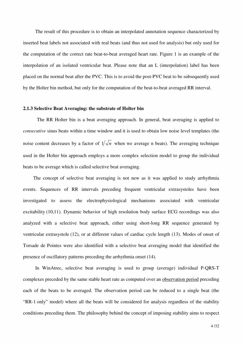
The result of this procedure is to obtain an interpolated annotation sequence characterized by

inserted beat labels not associated with real beats (and thus not used for analysis) but only used for

the computation of the correct rate beat-to-beat averaged heart rate. Figure 1 is an example of the

interpolation of an isolated ventricular beat. Please note that an L (interpolation) label has been

placed on the normal beat after the PVC. This is to avoid the post-PVC beat to be subsequently used

by the Holter bin method, but only for the computation of the beat-to-beat averaged RR interval.

2.1.3 Selective Beat Averaging: the substrate of Holter bin

The RR Holter bin is a beat averaging approach. In general, beat averaging is applied to

consecutive sinus beats within a time window and it is used to obtain low noise level templates (the

noise content decreases by a factor of n1 when we average n beats). The averaging technique

used in the Holter bin approach employs a more complex selection model to group the individual

beats to be average which is called selective beat averaging.

The concept of selective beat averaging is not new as it was applied to study arrhythmia

events. Sequences of RR intervals preceding frequent ventricular extrasystoles have been

investigated to assess the electrophysiological mechanisms associated with ventricular

excitability (10,11). Dynamic behavior of high resolution body surface ECG recordings was also

analyzed with a selective beat approach, either using short-long RR sequence generated by

ventricular extrasystole (12), or at different values of cardiac cycle length (13). Modes of onset of

Torsade de Pointes were also identified with a selective beat averaging model that identified the

presence of oscillatory patterns preceding the arrhythmia onset (14).

In WinAtrec, selective beat averaging is used to group (average) individual P-QRS-T

complexes preceded by the same stable heart rate as computed over an observation period preceding

each of the beats to be averaged. The observation period can be reduced to a single beat (the

“RR-1 only” model) where all the beats will be considered for analysis regardless of the stability

conditions preceding them. The philosophy behind the concept of imposing stability aims to respect

5 /32

the restitution curve of ventricular repolarization which demonstrates how full adaptation of QT

interval to changes in heart rate is only achieved after a time period that can be longer than a minute

(15). Thus, despite an identical RR interval, beats occurring "in the middle of heart rate changes"

may have a different repolarization shape than those occurring at stable heart rate. Most of all, they

will have a different QT duration. This phenomenon, known as hytesresis will be covered in details

in Section 3.

One simple way to define stability is to impose the averaged RR interval computed over the

observation period (RRPer) to match with the immediately preceding RR interval (RR -1):

RR -1 = RRPer ± th1 (1)

where th1 is a user-selectable threshold set by default to 15 msec. Alternatively, stability may

require the equivalence of RR intervals calculated over more subperiods, or imply the usage of

other variables such for example heart rate variability parameters (16). Recently, more sophisticated

definitions based on the usage of the best fit model applied on a per-case basis have been

proposed (17).

Given a rule of selection and the time period where to apply it (for example a circadian period

or a the peak concentration of a compound), the algorithm used in the Holter bin determines a

family of averaged templates, one per class of RR intervals (from here the terminology RR bins).

The stratification (bin) resolution is user selectable and can be as small as 10 milliseconds which is

appropriate for systems with high sampling rate. The total number of templates obtained within a

family depends on bin resolution and on the effective range of heart rates available in the time

period analyzed. Figure 2 summarizes the process of beat/selection allocation of Holter bin method:

starting from the RR interval measurements, individual beats are allocated (averaged) in the bin

whenever they meet the selection criterion imposed. At the end of the process, a single QT interval

6 /32

(or other quantitative parameter) is measured on the averaged waveform. Figure 3 shows a cascade

display of a family of templates together with the associated histograms of RR bins

2.1.4 Correcting the trigger jitter of annotation files

Commercial Holter systems implement proprietary algorithms and mathematical definitions

for QRS fiducial markers (for example the center of mass or maximum velocity in the QRS).

Because of these differences, consistency in the positioning of QRS fiducials cannot be assumed

a-priori. Even worse, a so-called trigger jitter effect, which can be defined as an inconsistent

positioning of the fiducial QRS markers (even between a beat and the next), is known to affect

many systems. Trigger jitter would typically produce larger (longer) and smaller (less amplitude)

QRS complexes. In addition, even the RR bin assignment would be affected as the sequence of RR

intervals would also be modified by a wrongly positioned fiducial point.

All methods that implement some form of beat averaging, thus including Holter bin, should

include proper signal pre-processing to avoid (or to correct for) trigger jittering. In WinAtrec, the

correction algorithm is based on a complete re-analysis of the QRSs positions and on the

application of a parabolic interpolation to reliably define the apex of the QRS complex of each

beat (16,18). Figure 4 is a real-case example where trigger jitter is overtly seen within a few

seconds of data; the strip in the upper part is extracted before the correction and the lower strip after

the correction. Figure 5 shows the effect of trigger jittering in an extreme case: the two overlaid

templates are the averages of QRS complexes from the same time window before (light pen) and

after (black pan) trigger jitter correction (from the same ECG subject of Figure 4). The before-

correction template is clearly affected by BOTH a distorted QRS (smaller amplitude plus an artifact

S wave) and even a T wave alteration. The importance of applying proper trigger jitter correction is

apparent.

7 /32

2.1.5 Proper beat alignment

Most commercial systems produce digital ECGs at a relatively low sampling rate (in the

range of 200 Hz). When performing beat averaging single beats need to be aligned (superimposed)

on the top of each other. This process, even when the effect of trigger jitter has been compensated,

can still determine small distortions in the averaged complexes, due to the random positioning of

the alignment (fiducial) markers associated with sampling rate.

To cope with this problem all individual beats to be averaged are oversampled (at 400 Hz)

and resynchronized with respect to the apex of the R-wave as estimated by the peak of the fitted

parabola (16,18). More details on the mathematic model used to perform this realignment can be

found in the original article that introduced selective beat averaging (16).

Of note, this resampling procedure is not applied with the aim to increase or to add

information (a purely utopian goal) but only with the intent to produce better alignment of

individual beats before averaging. To give a quantitative ballpark, on a commercial system with a

sampling rate in the range of 200Hz (i.e. digital samples 5 msec apart) an averaged complex

obtained without realignment can produce QRS complexes from 3 to 8 msec longer than that of the

individual beats used for the averaging (data extrapolated from WinAtrec validation

documentation).

2.1.6 Measurements on averaged waveforms versus beat-to-beat measurements.

Even after reducing the variability linked with heart rate variations (using bin stratification),

hysteresis (imposing stability) or autonomic factors (focusing on well-defined circadian periods),

some residual variability related to other factors (on for all the short-term respiratory related

variations) will still characterize the individual beats used for averaging. It is thus legitimate to

question how representative a measurement performed on an averaged waveform can be with

respect to the population of measurements from the individual beats used to obtained the averaged

waveform.

8 /32

WinAtrec validation addressed this specific issue on both real and on simulated data and we

will report three significant examples. In Figure 6a, results from a real case example are reported:

the distribution of beat-to-beat QT measurements is displayed together with the single-value

QT measurement (vertical line) obtained on the waveform derived averaging all the individual beats

from a 8-hour time window (12:00-20:00; RR interval range: 610-1230). In both cases (i.e. on

beat-to-beat and on the averaged waveform) the QT interval was measured by the same algorithm

implemented in WinAtrec used in fully-automatic (no user overreading) mode. In this algorithm,

the T wave offset definition is based on first derivative adaptive threshold (16).

Of note, the averaged waveform of this experiment was intentionally derived without using

any selection criteria (no RR bin stratification, no stability imposed), and thus maximizing all

sources of variability. Indeed, the range of QT intervals is fairly large and also contains the

algorithm “mistakes” (in the small tail of the left hand of the distribution, and above 500 msec on

the right hand). The range of beat-to-beat QT intervals typically seen with RR bin is of course much

smaller and reduced to only few milliseconds, particularly when a stable model is imposed.

The beat-to-beat distribution of Figure 6a is not symmetric and it has faster descend at

QT intervals higher than then mean value (423 msec) and with a small tail centred around 300

msec. The median and the mode (most frequent) values were respectively 420 and 411 msec. The

measurement derived from the averaged waveform was 410 msec thus reflecting the mode (most

frequent value) of the distribution.

The same behaviour is confirmed on simulated data. In Figure 6b and 6c, the distribution of

individual QT intervals was predetermined to have respectively a rectangular and a triangular shape

centred at 400 msec and covering the 350-450 msec range. Like in the real case example, the

QT interval measured on the averaged template matched with the mode of the distribution (which

for these two simulations also correspond the mean and median values).

These results indicate that from a pure mathematical standpoint, and at least with respect to

the measurement algorithm implemented in WinAtrec, measurements performed on the averaged

9 /32

waveform reflect the most frequent values of the measurements from the individual beats used for

the averaging, and thus are not biased by extremes values from the individual beat population.

2.2 Audit Trail of RR Holter bin

One of the big concerns with the implementation of Holter bin approach in clinical trials is

that of a proper audit trail on the individual beats used (averaged). For each period analyzed,

WinAtrec automatically generates a log file where a beat-to-beat report is stored. The log file

includes an header where user selectable options chosen are reported (for example the length of the

observation period, bin resolution, span of RR interval considered). The header is followed by a

beat-to-beat table where time of occurrence, beat label, RR interval, and bin allocation of each

individual beat in the analyzed period is reported. This table allows a-posteriori verification of

proper bin allocation and verification of proper beat exclusion (based on either beat labeling or on

stability criteria). The table is followed by a summary where basic statistics (total number of

included/excluded beats) and number of individual beats averaged in each bin are reported. Figure 7

is an extract of the Holter bin beat-to-beat report from a real case.

3. The hysteresis dilemma

Repolarization duration does not respond instantaneously to sudden heart rate changes and the

QT interval takes time to adapt to heart rate changes. This phenomenon is well known and has been

observed and described since many years (15). During exercise, hysteresis is very easily seen in the

QT/RR plane as the state map curves follow two completely separate patterns during the exercise

and the recovery phases (19). The most critical consequences of this phenomenon is that using the

preceding RR interval, either for correcting or even, as in our case, to decide bin allocation, may be

quite dangerous. In Figure 8, an ideal model for hysteresis is shown on the QT/RR plane (each

circle identifying a singe beat): in the centre we have a steady-state (QT1, RR1) pair. If we imagine

an ideal step increase in heart rate (i.e. a sudden acceleration) the RR interval will jump from RR1 to

10 /32

RR3 (RR3 < RR1 ) while the QT interval will take time to reach the new steady state value QT3.

During the adaptation phase QT intervals are longer than at steady state value QT3. Conversely, an

ideal step decrease in HR (a sudden deceleration), will trigger a jump increase in RR (RR2 > RR1 ),

and an adaptation phase with observed QT intervals shorter that the new steady state QT interval

(QT2). These shorter/longer QT intervals during adaptation times will have two major

consequences:

1) During adaptation, for a fixed RR interval we would observe several different values of QT

with a consequent altered correction mechanism (if we correct the QT interval). In the

context of an averaging approach such as the Holter bin, individual beats with different

QT intervals would be included in the same RR bin.

2) ANY QT/RR regression model fitted to all observed data would produce altered results

with weaker (less steep) slopes observed when keeping all (stable and unstable)

observations.

The model of Figure 8 is purely ideal, as we do not have sudden step changes in a daily

standard scenario (the closest we can get would be using pacemakers or running an exercise-test

protocol). On the other hand, the hypotheses derived can be verified on real data. Figure 8 has been

obtained from a normal subject with substantial physical activity during the recording. The

averaged RR interval in the period analyzed in the example was 700 msec (see the histogram in

upper right corner of the Figure). The superimposed waveforms shown in Figure 8 were obtained

respectively averaging all the beats with a preceding RR interval of 630 msec (dark pen waveform),

and only averaging the beats preceded by a stable heart rate (light pen waveform). Thus, the RR bin

shown (RR=630), corresponds to an heart rate faster than the mean heart rate of the explored period,

and potentially includes both steady-state values (for the RR=630 level) and adapting periods that

we could assume to be acceleration sequences. The “ALL” beat (unstable) waveform overtly shows

11 /32

a longer QT interval than the stable waveform, confirming the hypotheses of the model. Of note, the

number of averaged beats in the stable waveform is significantly smaller than that in the unstable

waveform (70 versus 151).

The example shown in Figure 9 was taken intentionally as an extreme case with “a lot” of

hysteresis (a normal subject which was active during the period analyzed). However, the same type

of results (observing shorter QT intervals whenever the heart rate is below the averaged heart rate

and longer QT intervals in heart rate ranges above the mean heart rate), can be confirmed in

general, although in many cases (particularly when the subject analyzed was forced to keep resting

condition by the clinical protocol) the differences between the stable and unstable model were

minimal.

Ideally, the amount of hysteresis should be quantified on a case by case basis and a stable

model should be imposed anytime the hysteresis would cross a certain threshold. Certainly, a good

way to minimize the problem would be to carefully define protocols aimed to minimize a-priori the

presence of hysteresis (for example limiting physical activity and make sure the ECGs analyzed

would be taken only after stable heart rate conditions).

What needs to be clear is that hysteresis is not a methodological pitfall of an approach more

than another, but rather a physiologic phenomenon that can affect the data on a case-by-case

magnitude. We strongly believe that the Holter bin method, through the intrinsic concept of

selective beat averaging, is actually one of the existing methods that better control the presence of

hysteresis. Clearly the price paid to take this into account can be that of excluding a significant

amount of beats that, depending on the definition of stability imposed, can become a big percentage

of total available data.

Table 1 reports the results from a real case example that help us to understand the price of

hysteresis. Data from the table are taken from a normal subject and are based on a 2-hour time

period (16:00-18:00),with an averaged heart rate of 60 beats per minute (RR=1000). The RR Holter

bin algorithm was run using a “RR-1 only” model (i.e. no control of hysteresis or all beats included)

12 /32

and using the stability criteria from section 2.1.3 with a progressively increasing observation period

(10, 20, 30 and 60 seconds). In the second column of the table the QT interval from the RR bin at

the averaged RR of the considered period (RR1000) is reported with (in parenthesis) the number of

individual beats averaged. Last columns also report the QT interval associated with two RR bins

away from the averaged RR, respectively RR1050 and RR950.

Model QTRR1000 (n) QT1050 (n) QT950 (n)

RR-1 only 345 (1406) 358 (318) 345 (213)

10 seconds 345 (1048) 360 (152) 345 (124)

20 seconds 345 (988) 360 (122) 343 (87)

30 seconds 345 (982) 362 (105) 343 (84)

60 seconds 345 (967) 362 (79) 340 (49)

Table I: The price of hysteresis

The price “paid” to impose stability is apparent. Even with a short observation period (10

seconds), the “loss” of beats is already significant, although more important (in percent) away from

the averaged RR (in the RR1000 bin the number of included beats changed from 1406 to 1048, a 25%

loss; in the RR1050 bin it changed from 318 to 152 beats, a 52% loss). This loss of beats

progressively augmented by increasing the length of the observation, although it was less

pronounced in the central RR bin. With 60 seconds observation period, the loss was 31%, 75%, and

77% respectively for the RR1000, RR950 and RR1050 bins, with an overall total loss of 842 beats out of

1937 initially available (43%). In the central (averaged RR) bin, the QT interval did not change with

the imposed stability whereas it progressively increased and decreased in the RR1050 and RR950 bins.

This observation is perfectly in line with the ideal model previously described, i.e. without

hysteresis control the QT interval is longer at faster heart rates (shorter RR intervals) and shorter at

lower heart rates (longer RR intervals).

In the Alfusozin study, the study that gave the visibility of this technology to the

pharmaceutical world, the Holter bin method was applied using the “only RR-1” model, i.e. without

13 /32

using the stable model and hysteresis was intentionally minimized at the protocol level (8). This

decision (whose discussion is beyond the scope of this chapter) led to some confusion and

criticisms which created the misconception that the Holter bin approach cannot correct hysteresis or

(even worse) that hysteresis is a problem specific to this method. All the arguments reported should

have clarified that this is definitely not the case.

4. QT/RR relation with the holter bin method

An intrinsic feature of the Holter bin method is that only a single QT interval will be derived

from a given RR interval. In the QT/RR plane this characteristics leads to a plot with a limited

number of QT/RR pairs (one per each bin). A thorough discussions on the advantages and problems

of this is beyond the scope of this chapter and has been exhaustively covered in literature. Actually,

the method itself was initially developed with the purpose of better assessing QT dynamicity, and in

particular the QT/RR relationship. The most important and well-accepted findings can be

summarized as follows:

• When the inspected period (i.e. the period where the method is applied) is well defined from

an autonomic nervous system perspective (for example avoiding to mix day and night) the

QT/RR relationship is strongly linear with high correlation coefficients (16,20,21,22)

• The relationship is stronger (i.e. steeper) if we focus on stable heart rate conditions. In other

words mixing stable heart rate and hysteresis periods lead to a different QT/RR

relationship (18). Figure 10 show the QT/RR plot from a real case example and are

extracted from a 4 hour period. In Figure 10a all the beats (n=19846) were included whereas

in Figure 10b a 60 seconds stability period was imposed (n=7412, i.e. almost 2/3 of total

beats were excluded). While remaining in both cases highly linear (r = 0.96), the slope of the

stable model was significantly steeper (again in perfect line with the model of Figure 7).

14 /32

Assessment of QT dynamicity has been one of the initial focuses of WinAtrec and several works

confirming the above statements have been published on the matter, both on healthy subjects

(20,23) and in pathological populations (21,22).

5. Working with RR bin templates: the serial approach

One of the strongest and most practical opportunities offered by the Holter bin approach is

certainly its intrinsic orientation toward serial analysis, i.e. toward the comparison of records taken

at different time points.

Indeed, the fact of sorting all the analyzed periods by heart rate and to obtain a single reference

waveform for each RR interval bin facilitates the superimposition and quantitative comparison of

templates obtained under different conditions during the same recording (for example day versus

night or comparison between periods with different drug concentrations), or across recordings taken

at separate time-matched periods (e.g. baseline versus drug). It is thus possible to compare

parameters and measurements from ECG waveforms from different periods (the so-called

comparison at identical heart rate), without the need to normalize or correct the observations (e.g.

the QT intervals) for heart rate changes.

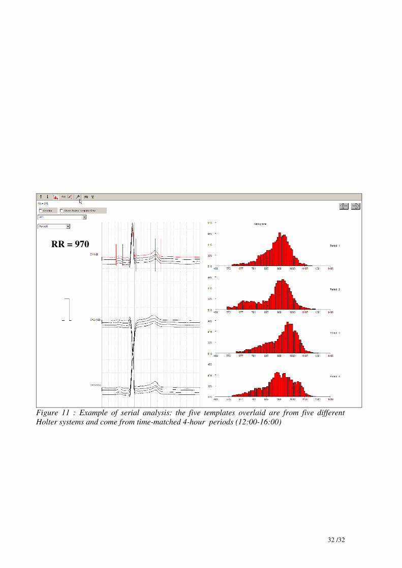
An example of this serial analysis comparison at identical heart rate is shown in Figure 11 where

ALL the templates (i.e. from all the families) of a given RR bin are overlaid. The user can make

direct assessment of the QT changes throughout the periods at the same heart rate.

In the example of the Figure, there are five separate time matched periods and the overlapped

templates are those associated to the bin RR = 970 (which is common to all five periods). User can

jump to the next or previous RR bin by using the arrow buttons in the upper right part of the screen.

The output of this comparison at identical heart rate is a serial table where each measurement

variable chosen for the analysis is repeated (columns) over each RR bin (rows). This worksheet

organization enables easy derivation of statistics (e.g. delta of variables when comparing)

15 /32

6. Limitations of Holter bin method and possible evolution

From a pharmacological point of view, the most relevant limitation of the Holter bin

approach is that long-enough period of stable conditions (in particular, plasma concentrations) are

required to populate an acceptable number of bins. This may become a problem with compounds

characterized by a fast response where important periods to be captured (such as the peak

concentration period) would be just too short to apply the method. Under these circumstances, a

more standard beat-to-beat approach, or even a time-based averaging applied over short durations

may be more suitable. WinAtrec can already generate time-based templates and apply the same type

of comparative analysis (in particular the serial approach described in section 5) available form the

Hotler RR bin method.

The architecture of the method facilitates the extension toward other selection criterion

models. For example, the selection of bins could be based on different physical activity periods with

the use of an activity status index, considering different sleep conditions (25) or focusing over

awakening periods (26). The support for these more sophisticated stratification criteria would

require additional biomedical sensors that could become available with continuous ECG recording.

Alternatively, selection could be driven by the occurrence of specific events, such as arrhythmias or

ischemia. As a future direction it may also be interesting to take into account, in addition to the

dependence of the actual QT value on a certain number of previous RR intervals, also the action of

inputs capable to modify QT interval independently of RR interval changes (27).

Last, the Holter bin approach should not be seen as a method limited to the analysis of

repolarization but rather as a technique suited for the quantitative analysis of electrocardiograms in

the broad sense. Interestingly enough, the first application of the method in a pharmaceutical

clinical trial was for the analysis of QRS intervals (see next section).

7. Holter bin method usage in pharmaceutical trials

16 /32

7.1 Usage of Holter bin method for assessment of drug-induced QT prolongation in class III

antiarrhytmic agent.

The objective of this study was to study the influence of heart rate on dofetilide-induced

QT prolongation among healthy volunteers (24). Ten healthy volunteers underwent two 24-hour

ECG recordings, one in the absence of dofetilide and the other after a single oral dose of 0.5 mg

dofetilide. Two 4-hour periods were defined during the second recording: Dh, which corresponded

to stable high concentration of the drug, and D1, which corresponded to low concentration of the

drug. Corresponding baseline recording periods, Ch and C1, matched by time with Dh and D1 were

selected from the control ECG recording in the absence of dofetilide. Rate-independent changes in

QT duration were analyzed using the Holter bin method with a 60 seconds stable model. The serial

comparison approach described on section 5 was used both to compare in-between recordings

(comparison between different concentration periods) and across recordings (baseline versus drug).

During Dh, dofetilide induced a mean 12% lengthening of ventricular repolarization.

Dynamic ECG analysis showed that this prolongation increased as RR intervals became longer, a

phenomenon known as reverse rate dependence. However, QT prolongation persisted at the shortest

(600 ms) RR intervals that could be analyzed. More interestingly, during D1, dynamic ECG

analysis showed a persistent, although small, effect of dofetilide on both QT prolongation (3%) and

reverse rate dependence of this effect. The study concluded that Dofetilide prolongs QT duration,

and this class III effect is influenced by heart rate. The Holter bin method was shown to be sensitive

to detect small changes during low concentration periods.

17 /32

7.2 Usage of Holter bin method for QRS interval changes assessment: the flecainide extended

release study.

This study was conducted in the Lariboisiere Hospital between 1999 and 2002 (7,28). The

goal of this trial was to inspect pharmacodynamic equivalence of flecainide acetate immediate-

release (IR) and controlled-release (CR) formulations as assessed from QRS duration in patients

previously treated with the IR formulation (ref). Patients were blindly randomized to the IR group

(100 mg b.i.d, n = 25) and to the CR group (200 mg o.d, n = 23) and ECG parameters were

measured at baseline and at Week 8 from 24-hour Holter.

The Holter bin approach was used to derive QRS interval durations at different classes of

constant RR intervals (bin resolution: 10 msec; stability period: 1 minute) over the entire 24 hours.

Using Hodges-Lehmann estimates of the difference between IR and CR groups for percent change

in QRS duration between baseline and Week 8 was 1.6% [-0.1; 3.7], indicating that both

formulations were pharmacodynamically equivalent. Median QRS values (102 ms versus 100.1 ms

at baseline; 103.15 ms versus 99 ms at week 8) as well as first and third quartiles were very similar

in both groups (Table II). The correlation between QRS duration and RR classes at baseline was

highly significant (p < 0.0001). The study conclusion was in favour of pharmacologic equivalence

between the two different concentration formulations.

Flecainide IR (N = 25)

Flecainide CR (N = 23)

Baseline (ms)

Median (ms) 102.00 100.10

Q1; Q3 (ms) 98.00; 110.38 95.43; 109.92

Week 8

Median (ms) 103.15 99.00

Q1; Q3 (ms) 98.00; 109.00 94.24; 105.36

% change between baseline and Week 8

Median 0.04 -0.5

Q1; Q3 -0.88; 2.74 -2.33; 0.92

Hodges-Lehman estimate [95% CI] 0.9 [-0.4; 2.2] -0.7 [-2.7; 0.2]

Hodges-Lehman estimate of

IR - CR [95% CI]

1.6 [-0.1; 3.7]

Q1; Q3: First and third quartiles. IR: Immediate-release formulation. CR: Controlled-release formulation.

95% CI: 95% confidence interval.

Table II: Results for the flecainide extended release study

18 /32

7.3 Usage of Holter bin method for QT interval changes assessment: the Alfusozin study

This crossover study included two single doses of the α1-adrenergic receptor blocker

alfuzosin, placebo and a QT-positive control arm (moxifloxacin 400 mg) in 48 healthy subjects (8).

Bazett, Fridericia, population-specific (QTcN) and subject-specific (QTcNi) correction formulae

were applied to 12-lead ECG recording data. QT1000 intervals (QT at RR=1000 msec) were

obtained from Holter recordings using custom software to perform time-matched, subject-specific,

rate-independent QT analysis.

The Holter bin approached was applied to analyze a 4-hour period centred around the peak

concentration of alfusozin. At the therapeutic dose (10 mg), alfuzosin did not induce any

significant change in the QT1000 (+0.1 msec 95%CI[-2.5;2.6]), QTcN (+0.5 msec

95%CI[-2.0;3.0]) or QTcNi intervals (+0.5 msec 95%CI[-2.0;2.9]). Alfuzosin at a supra maximal

dose 40 mg induced a small but significant QT1000 increase of 2.9 msec 95%CI[0.3;5.5]. This

increase was lower than that induced by moxifloxacin at the therapeutic dose (+7.0 msec

95%CI[4.4;9.6]). Alfuzosin 40 mg increased heart rate by 3.7 bpm, concordant with the greater

increase observed with the Bazett formula. The direct Holter-based QT interval measurement

method is sensitive to detect small drug-induced QT changes. Alfuzosin produced a slight non

significative increase in heart rate and did not significantly prolong QT interval at the therapeutic

dose. Alfuzosin's effect on QT interval at 4 times the therapeutic dose was less than 5 msec.

19 /32

References

1. Viskin S. Long QT syndromes and torsade de pointes. Lancet. 1999;354:1625-33.

2. Crouch MA, Limon L, Cassano AT. Clinical relevance and management of drug-related QT

interval prolongation. Pharmacotherapy. 2003;23:881-908.

3. Redfern WS, Carlsson L, Davis AS, Lynch WG, MacKenzie I, Palethorpe S et al. Relationships

between preclinical cardiac electrophysiology, clinical QT interval prolongation and torsade de

pointes for a broad range of drugs: evidence for a provisional safety margin in drug development.

Cardiovasc Res. 2003;58:32-45.

4. Vos MA, van Opstal JM, Leunissen JD, Verduyn SC. Electrophysiologic parameters and

predisposing factors in the generation of drug-induced Torsade de Pointes arrhythmias. Pharmacol

Ther. 2001;92:109-22.

5. Franz MR, Swerdlow CD, Liem LB, Schaefer J. Cycle length dependence of human action

potential duration in vivo: effects of single extrastimuli, sudden sustained rate acceleration and

deceleration, and different steady state frequency. J Clin Invest 1988;82:972-9.

6. Viitasalo M, Karjalainen J. QT Intervals at heart rates from 50 to 120 beats per minutes during

24-hour electrocardiographic recordings in 100 healthy men. Circulation 1992;86:1439-42.

7. Coumel P, Maison-Blanche P, Tarral E, Perier A, Milliez P, Leenhardt A. Pharmacodynamic

equivalence of two flecainide acetate formulations in patients with paroxysmal atrial fibrillation by

QRS analysis of ambulatory electrocardiogram. J Cardiovasc Pharmacol. 2003 May;41(5):771-9.

8. http://www.fda.gov/cder/foi/nda/2003/021287_uroxatral_toc.htm

9. Badilini F, "The ISHNE Holter Sandard Output File Format", A.N.E., 1998; 3(3):263-266.

10. Zimmermann M, Maison Blanche P, Cauchemez B, Leclercq JF, Coumel P Determinants of the

spontaneous ectopic activity in repetitive monomorphic idiopathic ventricular tachycardias. J Am

Coll Cardiol 1986; 7(6): 1219-1927.

11. Albrecht P, Cohen RJ, Mark RG. A stochastic characterization of chronic ventricular ectopic

activity. IEEE Trans Biomed Eng 1988; 35:539-50.

20 /32

12. Narayanaswamy S, Berbari EJ, Lander P, Lazzara R. Selective beat averaging and spectral

analysis of beat intervals to determine the mechanisms of premature ventricular contractions. In

Comp in Cardiology Proceedings 1993: 81-4.

13. Romberg D, Patterson H, Theres H, Lander P, Berbari R, Baumann G. Analysis of alternans in

late potentials. J Electrocardiol 1995; 28 (suppl): 198-201.

14. Locati E, Maison Blanche P, Dejode P, Cauchemez B, Coumel P. Spontaneous Sequences of

onset of Torsade de Pointes in patients with acquired prolonged ventricular repolarization:

quantitative analysis of Holter recordings. J Am Coll Cardiol 1995; 25: 1564-75.

15. Franz MR, Swerdlow CD, Liem LB, Schaefer J. Cycle length dependence of human action

potential duration in vivo: effects of single extrastimuli, sudden sustained rate acceleration and

deceleration, and different steady-state frequency. J Clin Invest 1988; 82: 972-9.

16. Badilini F, Maison-Blanche P, Childers R, Coumel P. QT interval analysis on ambulatory

electrocardiogram recordings: a selective beat averaging approach. Med Biol Eng Comput

1998:36:1-10.

17. Pueyo E, Smetana P, Hnatkova K, Laguna P, Malik M. Time for QT adaptation to RR changes

and relation to arrhythmic mortality reduction in amiodarone-treated patients. Proc in Computers in

Cardiology 2002; 565-8.

18 Merri M, Farden D, Mottely JG, Titlebaum EL. Sampling frequency of the electrocardiogram for

the spectral analysis of heart rate variability. IEEE Trans Biomed Eng 1990; 37: 99-106.

19 Sarma JSM, Venkataraman K, Samant DR, Cadgil U. Hysteresis in the human RR-QT

relationship during exercise and recovery. Pace 1987; 10: 485-491

20. Extramiana F, Maison-Blanche P, Badilini F, Pinoteau J, Deseo T, Coumel P. Circadian

modulation of QT rate dependence in healthy volunteers. J Electrocardiol 1999;32:33-43.

21. Extramiana F, Neyroud N, Huikuri HV, Koistinen MJ, Coumel P, Maison-Blanche P. QT

interval and arrhythmic risk assessment after myocardial infarction. Am J Cardiol 1999;83:266-269.

21 /32

22. Extramiana F, Maison-Blanche

P, Tavernier

R, Jordaens

L, Leenhardt

A, Coumel

P. Cardiac

effects of chronic oral beta-blockade: lack of agreement between heart rate and QT interval

changes. Ann Noninvasive Electrocardiol. 2002;7:379-388.

23. Lande G, Funck-Brentano C, Ghadanfar M, Escande D. Steady-state versus non-steady-state

QT-RR relationships in 24-hour Holter recordings. Pacing Clin Electrophysiol. 2000

Mar;23(3):293-302.

24. Lande G, Maison-Blanche P, Fayn J, Ghadanfar M, Coumel P, Funck-Brentano C. Dynamic

analysis of dofetilide-induced changes in ventricular repolarization. Clin Pharmacol Ther. 1998

Sep;64(3):312-21.

25. Verrier RL, Stone PH, Pace-Schott EF, Hobson A. Sleep related cardiovascular risk: new home-

based monitoring technology for improved diagnosis and therapy. A.N.A. 1997; 2:158-75.

26. Toivonen L, Helenious K, Vitasalo M. Electrocardiographic replarization durino stress from

awakening on alarm call. J Am Coll Cardiol 1997;30:774-9.

27. Porta A, Baselli G, Caiani E, Malliani A, Lombardi F, Cerutti S, Quantifying electrocardiogram

RT-RR variability interactions, Med. Biol. Eng. Comput., 1998, 36, pp. 27-34.

28. Badilini F, Blanche PM, Ngo P, Coumel P, Leenhardt A. Computerized QRS analysis from 24

hour ambulatory monitoring to assess pharmacodynamic changes. J Electrocardiol. 2003;36

Suppl:109-10.

22 /32

Figure 1: Example of interpolation: The two L-labelled beats will not be used by the RR bin method

but only for the computation of the beat-to-beat averaged heart rate.

23

/3

2

������

����

����

�����

���

�����

����

�����

�����

�����

�« ��

� »�

����

����

����

���

����

����

����

���

�

�����

����

�� ��

�����

�����

����

����

�����

��� ��

�����

������

��

������

�� �����

����

�����

�����

�����

����

�� � ����� � ����� ����� ������ � ����� � ����

��� ����F

igu

re 2

24 /32

Figure 3: Cascade display of a family of RR bin templates with the associated histogram

25 /32

Figure 4: ECG strip shown before (upper panel) and after (lower panel) jitter correction. Before

correction, the positioning of beat labels fluctuates form one beat to another whereas after

correction they are stabilized. Even the RR interval sequence is seriously affected with changes up

to 100 msec long.

26 /32

Figure 5: averaged complexes from the ECG of Figure X-1. The waveform in light is that obtained

averaging beats before jitter correction; the bold waveform is the that obtained averaging the same

beats after correction. The distortions (resulting is a smaller and wider QRS and in a longer QT

intervals) are apparent.

smaller QRS

longer QT wider QRS

27 /32

A

0

10

20

30

40

50

60

70

320 340 360 380 400 420 440 460 480

B

0

10

20

30

40

50

60

70

80

C

Figure 6: Comparison between beat-to-beat distributions and single-value (from the averaged

waveform) of QT intervals from a real case example (panel A) and from two simulation

experiments based on triangular (panel B) and rectangular (panel C) beat-to-beat distributions.

� ���� �������� �������� � ��������������� � �� ����!���"

������������ � �� ����!���" � ���� �������� �������� � ��#

350 450

� ���� �������� �������� � �#�

28 /32

Figure 7: Extract of Holter bin beat-to-beat report

beat- by beat report

Summary of bin

analysis

Summary

Statistics

29

/3

2

RR

1

RR

2

RR

3

dec

eler

atio

n

Sta

ble

pai

r (Q

T1, R

R1)

Adap

tati

on p

has

e

Unst

able

pai

rs

Sta

ble

pai

r (R

R2, Q

T2)

RR

1,Q

T1

RR

3,Q

T3

RR

3, Q

Tad

apt.

> Q

T3

RR

Q

T

ac

cele

rati

on

Sta

ble

pai

r (R

R3, Q

T3)

Adap

tati

on p

has

e

Unst

able

pai

rs

RR

1,Q

T1

RR

Q

T

“ST

AB

LE

” S

LO

PE

“UN

ST

AB

LE

” S

LO

PE

RR

2, Q

Tad

apt.

< Q

T2

Fig

ure

8

QT

RR

2,Q

T2

QT

1

QT

2

QT

3

QT

RR

30

/3

2

RR

= 7

00

RR

= 6

30

63

063

0

unst

able

stab

le

RR

< R

R

=>

QT

un

stab

le >

QT

stab

le

Per

iod

: 1

4:0

0 -

16

:00

Sam

e E

CG

, sa

me

tim

e p

erio

d,

On

ly d

iffe

ren

ce i

n u

sag

e o

f st

able

mo

del

Fig

ure

9

31 /32

Figure 10: QT/RR plots using the “RR-1 only” model with all beats included (panel A), and using

60 second stable model (panel B)

N = 19846

N = 7412

32 /32

Figure 11 : Example of serial analysis: the five templates overlaid are from five different

Holter systems and come from time-matched 4-hour periods (12:00-16:00)

RR = 970