ACTAUNIVERSITATIS

UPSALIENSISUPPSALA

2018

Digital Comprehensive Summaries of Uppsala Dissertationsfrom the Faculty of Science and Technology 1675

Holographic Wilson Loops

Quantum String Corrections

DANIEL RICARDO MEDINA RINCON

ISSN 1651-6214ISBN 978-91-513-0350-5urn:nbn:se:uu:diva-349210

Dissertation presented at Uppsala University to be publicly examined in Room FB53,AlbaNova Universitetscentrum, Roslagstullsbacken 21, Stockholm, Wednesday, 13 June2018 at 10:30 for the degree of Doctor of Philosophy. The examination will be conductedin English. Faculty examiner: Professor Gianluca Grignani (Università di Perugia).

AbstractMedina Rincon, D. R. 2018. Holographic Wilson Loops. Quantum String Corrections.Digital Comprehensive Summaries of Uppsala Dissertations from the Faculty of Science andTechnology 1675. 67 pp. Uppsala: Acta Universitatis Upsaliensis. ISBN 978-91-513-0350-5.

The gauge-string duality has been one of the most exciting areas in theoretical physics as itconnects strongly coupled field theories with weakly interacting strings. The present thesisconcerns the study of Wilson loops in this correspondence. Wilson loops are observables arisingin many physical situations like the propagation of particles in gauge fields, the problem ofconfinement, etc. In the gauge-string correspondence these observables have a known physicaldescription at both sides, making them ideal probes for the duality. Remarkable progressfrom localization has lead to predictions at all orders in the coupling for certain Wilson loopconfigurations in supersymmetric field theories. Being the string theory weakly interacting, inprinciple we can use perturbation theory to calculate the corresponding quantities. However,current string calculations have only been successful at leading order and in rare cases, nextto leading order. At next to leading order the difficulties encountered include divergences,ambiguous boundary conditions, mismatch with field theory results, etc. The research presentedin this thesis aims at a better understanding of these issues. The first calculation presented hereconcerns the Wilson line in N=2*, a massive deformation of N=4 SYM. The string theory dualto this configuration is a straight line in the type IIB Pilch-Warner background. Using techniquesfor functional determinants, we computed the 1-loop string partition function obtaining perfectmatching with localization. This constitutes a first test of the correspondence at the quantumlevel for nonconformal theories. The second calculation in this thesis corresponds to the ratioof the latitude and circular Wilson loops in AdS5xS5. An IR anomaly related to the singularnature of the conformal gauge is shown to solve previously found discrepancies with field theoryresults.

Keywords: Gauge-string correspondence, AdS/CFT, Wilson loops, String theory

Daniel Ricardo Medina Rincon, Department of Physics and Astronomy, Theoretical Physics,Box 516, Uppsala University, SE-751 20 Uppsala, Sweden.

© Daniel Ricardo Medina Rincon 2018

ISSN 1651-6214ISBN 978-91-513-0350-5urn:nbn:se:uu:diva-349210 (http://urn.kb.se/resolve?urn=urn:nbn:se:uu:diva-349210)

Dedicated to my parents and my sister

List of papers

This thesis is based on the following papers, which are referred to inthe text by their Roman numerals.

I X. Chen-Lin, D. Medina-Rincon and K. Zarembo, QuantumString Test of Nonconformal Holography, JHEP 1704 (2017) 095,[arXiv:1702.07954 [hep-th]].

II A. Cagnazzo, D. Medina-Rincon and K. Zarembo, Stringcorrections to circular Wilson loop and anomalies, JHEP 1802(2018) 120, [arXiv:1712.07730 [hep-th]].

Papers not included in the thesis

III G. Arutyunov, M. Heinze and D. Medina-Rincon, Integrability ofthe η-deformed Neumann-Rosochatius model, J. Phys. A 50(2017) no.3 035401, [arXiv:1607.05190 [hep-th]].

IV G. Arutyunov, M. Heinze and D. Medina-Rincon,Superintegrability of Geodesic Motion on the Sausage Model, J.Phys. A 50 (2017) no.24 244002, [arXiv:1608.06481 [hep-th]].

V D. Medina-Rincon, A. A. Tseytlin and K. Zarembo, Precisionmatching of circular Wilson loops and strings in AdS5 × S5,arXiv:1804.08925 [hep-th].

Reprints were made with permission from the publishers.

Contents

1 Introduction . . . . . . . . . . . . . . . . . . . . . . . . . . . . . . . . . . . . . . . . . . . . . . . . . . . . . . . . . . . . . . . . . . . . . . . . . . . . . . 9

2 String theory in curved backgrounds . . . . . . . . . . . . . . . . . . . . . . . . . . . . . . . . . . . . . . . . 132.1 Green-Schwarz type IIB superstring . . . . . . . . . . . . . . . . . . . . . . . . . . . . . . . . 132.2 Strings on AdS5 × S5

. . . . . . . . . . . . . . . . . . . . . . . . . . . . . . . . . . . . . . . . . . . . . . . . . . . . . 162.3 The Pilch-Warner background . . . . . . . . . . . . . . . . . . . . . . . . . . . . . . . . . . . . . . . . 17

3 Wilson loops in AdS/CFT . . . . . . . . . . . . . . . . . . . . . . . . . . . . . . . . . . . . . . . . . . . . . . . . . . . . . . . 203.1 The AdS/CFT duality . . . . . . . . . . . . . . . . . . . . . . . . . . . . . . . . . . . . . . . . . . . . . . . . . . . . 213.2 Wilson loops in field theory . . . . . . . . . . . . . . . . . . . . . . . . . . . . . . . . . . . . . . . . . . . . 223.3 Wilson loops in string theory . . . . . . . . . . . . . . . . . . . . . . . . . . . . . . . . . . . . . . . . . . 23

3.3.1 The classical action . . . . . . . . . . . . . . . . . . . . . . . . . . . . . . . . . . . . . . . . . . . . 253.3.2 The semiclassical partition function . . . . . . . . . . . . . . . . . . . . 26

3.4 Loop configurations . . . . . . . . . . . . . . . . . . . . . . . . . . . . . . . . . . . . . . . . . . . . . . . . . . . . . . . . 283.4.1 The Wilson line . . . . . . . . . . . . . . . . . . . . . . . . . . . . . . . . . . . . . . . . . . . . . . . . . 283.4.2 The circular Wilson loop . . . . . . . . . . . . . . . . . . . . . . . . . . . . . . . . . . . . 293.4.3 The latitude Wilson loop . . . . . . . . . . . . . . . . . . . . . . . . . . . . . . . . . . . . 30

4 Functional determinants . . . . . . . . . . . . . . . . . . . . . . . . . . . . . . . . . . . . . . . . . . . . . . . . . . . . . . . . . . 324.1 Zeta function & heat kernel . . . . . . . . . . . . . . . . . . . . . . . . . . . . . . . . . . . . . . . . . . . . 334.2 Determinants & conformal factors . . . . . . . . . . . . . . . . . . . . . . . . . . . . . . . . . . . 354.3 Isospectral operators . . . . . . . . . . . . . . . . . . . . . . . . . . . . . . . . . . . . . . . . . . . . . . . . . . . . . . 374.4 Phaseshifts & determinants . . . . . . . . . . . . . . . . . . . . . . . . . . . . . . . . . . . . . . . . . . . . 38

5 Wilson line in the Pilch-Warner background . . . . . . . . . . . . . . . . . . . . . . . . . . . . . 415.1 The classical partition function . . . . . . . . . . . . . . . . . . . . . . . . . . . . . . . . . . . . . . . 415.2 The semiclassical partition function . . . . . . . . . . . . . . . . . . . . . . . . . . . . . . . . 42

5.2.1 Bosonic operators . . . . . . . . . . . . . . . . . . . . . . . . . . . . . . . . . . . . . . . . . . . . . . . 425.2.2 Fermionic operators . . . . . . . . . . . . . . . . . . . . . . . . . . . . . . . . . . . . . . . . . . . 435.2.3 Putting everything together . . . . . . . . . . . . . . . . . . . . . . . . . . . . . . . . 45

5.3 The spectral problems . . . . . . . . . . . . . . . . . . . . . . . . . . . . . . . . . . . . . . . . . . . . . . . . . . . . 465.4 Numerics . . . . . . . . . . . . . . . . . . . . . . . . . . . . . . . . . . . . . . . . . . . . . . . . . . . . . . . . . . . . . . . . . . . . . . . 48

6 Ratio of latitude and circular Wilson loops in AdS5 × S5. . . . . . . . . . 50

6.1 The classical partition function . . . . . . . . . . . . . . . . . . . . . . . . . . . . . . . . . . . . . . . 516.2 The semiclassical partition function . . . . . . . . . . . . . . . . . . . . . . . . . . . . . . . . 51

6.2.1 The phaseshifts . . . . . . . . . . . . . . . . . . . . . . . . . . . . . . . . . . . . . . . . . . . . . . . . . . 536.2.2 Invariant regulators . . . . . . . . . . . . . . . . . . . . . . . . . . . . . . . . . . . . . . . . . . . . 56

6.2.3 Conformal factors . . . . . . . . . . . . . . . . . . . . . . . . . . . . . . . . . . . . . . . . . . . . . . 576.3 Putting everything together . . . . . . . . . . . . . . . . . . . . . . . . . . . . . . . . . . . . . . . . . . . . 58

7 Conclusions and open problems . . . . . . . . . . . . . . . . . . . . . . . . . . . . . . . . . . . . . . . . . . . . . . . . 59

Acknowledgments . . . . . . . . . . . . . . . . . . . . . . . . . . . . . . . . . . . . . . . . . . . . . . . . . . . . . . . . . . . . . . . . . . . . . . . . . 61

Svensk sammanfattning . . . . . . . . . . . . . . . . . . . . . . . . . . . . . . . . . . . . . . . . . . . . . . . . . . . . . . . . . . . . . . . . 62

References . . . . . . . . . . . . . . . . . . . . . . . . . . . . . . . . . . . . . . . . . . . . . . . . . . . . . . . . . . . . . . . . . . . . . . . . . . . . . . . . . . . . 64

1. Introduction

The research presented in this thesis concerns string theory and quantumfield theory in the framework of the gauge-string correspondence. Thiscorrespondence has been one of the most exciting areas in theoreticalphysics for the last decades and basically states the equivalence betweencertain quantum field theories and string theory in curved background.On one side of the correspondence we have gauge field theories, theyare quantum field theories which have a “gauge group” as a symmetry,and which constitute the building blocks of the Standard Model andof our current understanding of the universe. On the other side of thecorrespondence is string theory, a candidate for a theory of quantumgravity and an area which has enriched various fields of mathematicsover the years.

The prime example of the gauge-string correspondence is the so-calledAdS/CFT duality put forward by Maldacena [1], which proposes theexact correspondence between string theory in AdS5 × S5 and N = 4supersymmetric Yang-Mills (SYM). One of the remarkable features ofthe proposal is that it connects two theories with different dimension-ality: A string theory in five-dimensional Anti-de Sitter space and afour-dimensional field theory living in its boundary. But even more sur-prising is the fact that the map between the two theories is such thatN = 4 SYM at large values of the coupling constant is mapped toweakly coupled strings. This phenomenon has significant implicationsas some of the most challenging problems in field theory involve strongcoupling, a regime where perturbation theory proves insufficient. There-fore, through this duality we can gain new insights into strongly-coupledquantum field theories by studying string theory in curved background.

At present moment the AdS/CFT duality remains a conjecture, asthere is no mathematical proof despite the large amount of evidence sup-porting it. However, its possible implications in physics and mathemat-ics can not be overstated as it could give us new insights into strongly-coupled phenomena like the confinement of quarks and the descriptionof the mass spectrum of hadronic particles, a problem for which there isno theoretical explanation and is considered by the Clay MathematicalInstitute to be among the seven Millennium Prize problems.

The focus of the present thesis is in further developing the tools forthe string theory computation of a certain class of observables: Wilson

9

loops. In quantum field theory Wilson loops are observables arising inmany physical situations like the propagation of particles in the presenceof gauge fields and are also very convenient for understanding stronglycoupled phenomena, like confinement. Mathematically, they are definedthrough the trace of a path-ordered exponential transported along acontour C. There are several techniques for the calculation of thesequantities in field theory, for instance perturbation theory or latticesimulations using computers. However, if one desires a better analyticunderstanding of these observables at strong coupling, a regime whereperturbation theory breaks down, it is necessary to use more sophisti-cated techniques. Due to the strong/weak nature of the gauge-stringcorrespondence, insights into this type of computations for a stronglycoupled field theory can be achieved by computing the correspondingquantities in weakly coupled string theory.

As beautiful as this idea sounds, in practice it is very difficult asstring theory in curved backgrounds has many open questions and evenin perturbation theory only the first and, in very few backgrounds andconfigurations, second (also called 1-loop) terms have been successfullycomputed. In the string theory formalism, the dual to the Wilson loopis given by the path integral of a string which ends on a curve C at theboundary of AdS. At first order in the coupling parameter, contributionscome from the string action evaluated at a classical solution. Meanwhile,the 1-loop term comes from the contribution of second-order fluctuationsaround the classical solution, a problem which in principle reduces tothe evaluation of determinants of differential operators. The difficultiesin this type of calculations are many, both from a technical standpoint(divergencies, possible zero-modes, choice of boundary conditions, etc.)and from a conceptual point of view as string theory has not only manyfields, but also many symmetries, making the evaluation of the pathintegral difficult as double counting must be avoided.

Fortunately, due to remarkable progress in the field theory side com-ing from the use of localization and matrix models [2], there are exactpredictions at all orders in the coupling constant for a few cases wherethe field theory and the Wilson loop have a very high degree of symme-try. These cases provide an ideal set up to deepen our understandingof how these computations should be done in string theory and serveas perfect tests for new techniques. The hope is that by learning fromthese computations, we can extend our knowledge of perturbative stringtheory calculations further and eventually make predictions for stronglycoupled field theories.

The simplest Wilson loop configuration there is corresponds to a stringwhose geometry is a straight line in Anti-de Sitter space, also calledWilson line. This configuration has a trivial expectation value when the

10

field theory in question is N = 4 SYM: 〈W 〉 = 1. The later is due tothe large amount of supersymmetry preserved by this configuration as itis 1/2 BPS, thus preserving 16 Poincare supercharges. From the stringtheory perspective, this configuration was first studied for the case ofAdS5 × S5 in the pioneering work [3], where the expectation value ofthe Wilson line was computed up to 1-loop in string theory obtainingperfect matching with the field theory prediction.

This test of the AdS/CFT duality, as well as the related technicalmachinery developed for string theory in curved backgrounds, opensthe door to the possibility of testing other gauge-string dualities. Thequantum field theory described by N = 4 SYM is in a way a “toy model”of the field theories describing our universe, as N = 4 SYM has a largeamount of supersymmetry and has conformal symmetry. As a “toymodel”, N = 4 SYM is very useful since it is a perfect testing ground inwhich to test approaches to more complex theories, but at the end of theday one would like to extend current techniques to field theories closerto reality. One such theory is N = 2∗ Yang-Mills, a cousin of N = 4SYM whose field content has a massive multiplet breaking conformalsymmetry. This field theory has a string theory dual, the so-called Pilch-Warner background [4, 5], which is a distant cousin of AdS5 × S5 witha considerably more complicated field content. Unlike AdS5 × S5, thePilch-Warner background is not integrable making calculations in thisstring theory a very non-trivial task.

Despite the much more complicated field content and the technical dif-ficulties involved, in paper I we successfully calculated the 1-loop contri-bution to the string partition function corresponding to the Wilson linein the Pilch-Warner background and showed its divergence-free nature.By making use of methods from spectral functions, theory of differentialoperators and identities for isospectral operators, we managed to dra-matically simplify the calculation and reproduce the field theory resultof [6]. Furthermore, with these new mathematical tools in hand, wereproduced the earlier result for the Wilson line in AdS5 × S5 [3, 7] inan elegant and relatively simple manner. The perturbative calculationin I, first of its kind for nonconformal theories, serves as a showcasefor the power of spectral function methods in string theory Wilson loopcalculations. Moreover, it paves the way for precision testing of thegauge-string correspondence for nonconformal theories.

The second simplest Wilson loop configuration is perhaps a circularWilson loop in AdS, a problem whose all-loop answer is known fromfield theory but whose string theory calculation in AdS5 × S5 at 1-loophas been an open question for almost a decade. In the field theory side,the result at all orders in perturbation theory was first conjectured inthe foundational work [8], and then proven using localization in [2]. In

11

the string theory side of the duality, the picture is much less clear asseveral attempts coming from Gel’fand Yaglom [9, 10] and heat kernelmethods [7] had led to diverging results and mismatch with field theorypredictions. These perplexing results suggest that perhaps the tech-niques used, or the way they are implemented, are not adequate for theproblem at hand. Possible explanations of why past calculations havefailed are also attributed to the possibility of zero-modes of the “ghost”operators appearing from the gauge fixing procedure, or ignorance onwhat are the right boundary conditions of these spectral problems. Fur-thermore, if one considers the circle to have a winding k, the situationgets even worse as previous calculations have all found different results[9, 11].

In order to leave the question of ghost zero-modes aside, whose contri-butions are related to the string world-sheet geometry, previous studiesconsidered the ratio of two circular Wilson loops: the one mentionedabove living entirely on AdS and at a point in S5, and one which ad-ditionally extends in a S2 ⊂ S5 describing a latitude. Using Gel’fandYaglom, previous independent perturbative 1-loop computations failedto reproduce the results from localization in field theory [12, 13], and aperturbative heat kernel approach only reproduced the first term in a se-ries expansion of the 1-loop result for small latitude angle [14]. Recently,a similar computation using zeta function regularizarion also obtaineda mismatch with the field theory prediction [15]. In paper II, usingcontour integration methods and the spectral function methods appliedpreviously in the Pilch-Warner calculation of paper I, we obtained thesame 1-loop result as existing Gel’fan Yaglom computations [12, 13] plusan additional contribution, successfully solving this open problem. Theadditional piece at the heart of the problem comes from careful consider-ation of the conformal transformation required for the evaluation of thefunctional determinants in the cylinder. This beautiful result highlightsthe importance and desperate need for a better understanding of themathematical machinery required for these perturbative string theorycalculations.

This thesis is organized as follows: In chapter 2 the basic string theoryconcepts required are introduced, in chapter 3 Wilson loops are intro-duced in the context of the gauge-string correspondence. Chapter 4briefly reviews several techniques used for the computation of functionaldeterminants. Chapters 5 and 6 concern the string theory 1-loop compu-tation of the straight line in the Pilch-Warner background and the ratioof latitude and 1/2 BPS circular Wilson loops in AdS5 × S5. Finally, inchapter 7 the main results are summarized and several open problemsare mentioned.

12

2. String theory in curved backgrounds

Originally, string theory started in the 1960’s as a model of hadrons butit later became apparent that this theory could describe a consistenttheory of quantum gravity. General relativity, the theory which explainsgravitational interactions, is (at least perturbatively) non-renormalizablewhich is a problematic issue as it would require the introduction of in-finitely many parameters to absorb divergences. The later problem canbe solved by the radical proposal of replacing point-like particles by one-dimensional objects called “strings”. This proposal leads to a smootherUV behaviour and the existence of a massless spin two particle called“graviton” which interacts according to covariance laws of general rela-tivity. Besides being a consistent theory of quantum gravity perturba-tively, string theories lead to gauge groups that can include the StandardModel, consequently opening the exciting possibility of unifying gravityand the other fundamental forces under a single theoretical framework.

In addition to the mathematical consistency and possibilities of grandunification, string theory exhibits many interesting features to be stud-ied. Among these are the existence of extra dimensions, supersymmetryand dualities. String theory has several formulations connected by anintricate web of dualities. In the present thesis we will focus exclusivelyon type IIB string theory as this is the one relevant for the calcula-tions presented later. We will start by introducing this string theoryin the Green-Schwarz formulation in section 2.1. Later in sections 2.2and 2.3, we present the two supergravity backgrounds considered in ourcalculations: AdS5×S5 and the Pilch-Warner background, respectively.

2.1 Green-Schwarz type IIB superstring

A string is described by a 1+1 dimensional “worldsheet” moving in a10 dimensional “target space” (see examples in figure 2.1). The coordi-nates along the worldsheet will be denoted by τ and σ, where τ is theproper time coordinate while σ is the spatial coordinate along the string.The metric tensor along the worldsheet will be denoted by hij where{i, j} ∈ {1, 2}, while in the target space the coordinates are denoted by

13

Figure 2.1. Wordsheets of an open spinning string and of a closed string.

Xμ = Xμ(τ, σ) and the metric tensor by Gμν with {μ, ν} ∈ {1, .., 10}.The most general bosonic Lagrangian density is given by

LB =1

2

√hhij∂iX

μ∂jXνGμν +

i

2εij∂iX

μ∂jXνBμν , (2.1)

where the worldsheet metric is in Euclidean signature, Gμν is the tar-get space metric in the string frame and Bμν is an antisymmetric B-field.

Additionally, there is a term coupling the dilaton Φ to the worldsheetmetric

LFT =1

4π

√hR(2)Φ, (2.2)

where R(2) denotes the worldsheet Ricci scalar. The role of this term,usually referred as Fradkin-Tseytlin term, is not fully understood in theliterature for the case of the Green-Schwarz string [16] but will play akey role in the computation of paper I. The bosonic action resultingfrom both of these contributions is

SB =

∫d2σ

(√λ

2πLB + LFT

). (2.3)

The fermionic action for the Green-Schwarz string in a generic back-ground is known perturbatively up to fourth order in fermions [17], how-ever, for our purposes it is sufficient to consider the expression up to

14

second order. For the type IIB superstring this fermionic piece is [16]

L(2)F = ΨI

(√hhijδIJ + iεijτ

IJ

3

)/Ei

(δJKDj +

τJK

3

8∂jX

νHνρλΓρλ

+eΦ

8FJK /Ej

)ΨK . (2.4)

In the expression above H is the NS-NS three-form and the fermionic field ΨI

with I ∈ {1, 2} is a 32-component Majorana-Weyl spinor subject to the con-straint Γ11ΨI = ΨI . We use the notations /Ei = ∂iX

μEμνΓν and Γμ1μ2...μn =

Γ[μ1Γμ2 ...Γμn] where Eμν is the veilbein and Γμ are Dirac matrices, while Dj

and FJK are defined by [16]

Dj = ∂j +1

4∂jX

μωμαβΓαβ ,

FJK =

2∑n=0

1

(2n+ 1)!F

μ1μ2...μ2n+1

(2n+1) Γμ1μ2...μ2n+1σJK(2n+1) ,

where F(i) are the R-R field strengths, ωμαβ denotes the spin-connection and

σ(n) are 2× 2 matrices defined in terms of the Pauli matrices τi by

σ(1) = −iτ2 , σ(3) = τ1 , σ(5) = − i

2τ2 .

In order to notationally distinguish target space indices and those of its cor-responding tangent space, we have added a hat to the later. Naturally, thehatted and unhatted indices are connected by means of the vielbein Eν

μ.

The NS-NS three-form is defined by H = dB, while the R-R fluxes are givenin terms of the superpotentials C(i) by

F(1) = dC(0),

F(3) = dC(2) + C(0)dB,

F(5) = dC(4) + C(2) ∧ dB,

where the five-form is self-dual ∗F(5) = F(5) and the fluxes satisfy the Bianchiidentities

dF(i) = F(i−2) ∧ dB ∀i ∈ {3, 5}.In order to consistently define a supergravity background in which strings prop-agate, one must specify its field content which for the type IIB case amountsto

Gμν , Bμν , Φ, F(1), F(2), F(5),

which must satisfy the supergravity equations.

15

Figure 2.2. Images of anti-de Sitter space and the sphere.

Naturally, the string action resulting from equations (2.1), (2.2) and (2.4),has many symmetries including invariance under Poincare transformations,reparametrizations of the worldsheet, Weyl transformations and κ-symmetry.These symmetries can be used to choose a convenient gauge where for instancethe worldsheet metric is diagonal and the fermionic degrees of freedom arereduced in half, as will be discussed later.

2.2 Strings on AdS5 × S5

As discussed earlier, superstrings propagate in 10 dimensional supergravitybackgrounds. For type IIB supergravity the most studied example is perhapsAdS5 × S5 due to the prominent role it plays in the AdS/CFT duality. Here,we will briefly review its geometry, field content and its symmetries.

The metric of AdS5 in Poincare coordinates is written as

ds2AdS =1

z2(dx2

μ + dz2), (2.5)

where μ = {1, .., 4} and z � 0.Meanwhile, in Hopf coordinates S5 is described by

ds2S = dψ2 + sin2ψ dϕ2 + cos2ψ(dφ2

3 + cos2φ3 dφ21 + sin2φ3 dφ

22

), (2.6)

where {ψ, φ3} ∈ [0, π2

]and {ϕ, φ1, φ2} ∈ [0, 2π).

16

In order to visualize these spacetimes more easily, it is sometimes convenientto use “global coordinates” given by [18]

X1 + iX2 = sinψ cosφ3eiφ1 ,X3 + iX4 = sinψ sinφ3e

iφ2 , X5 + iX6 = cosψeiϕ,

Yn =xn

z∀n ∈ {0, ..., 3} , Y4 =

−1 + z2 + x2μ

2z, Y5 =

1 + z2 + x2μ

2z.

In these coordinates the metric tensors of (2.5) and (2.6) can be written as

ds2AdS = ηMNdYMdYN with ηMN = (−1,+1, ...,+1,−1) ,

ds2S = δMNdXMdXN with δMN = (+1,+1, ...,+1,+1) ,

with the coordinates satisfying

δMNXMXN = 1, −ηMNYMYN = 1.

In figure 2.2 the AdS2 and S2 spacetimes are presented in these coordinates.

The field content of AdS5 × S5 is relatively simple since the only non-zerofield besides Gμν is the R-R five-form F(5). The later takes the value

F(5) =1

z5dx0 ∧ dx1 ∧ dx2 ∧ dx3 ∧ dz

+ sinφ3 cosφ3 sinψ cos3ψ dψ ∧ dϕ ∧ dφ1 ∧ dφ2 ∧ dφ3.

Mathematically, AdS5 and S5 can be seen as the cosets

AdS5 =SO (4, 2)

SO (4, 1), S5 =

SO (6)

SO (5),

where in order to include fermions one replaces the orthogonal groups with spingroups. In general, type IIB superstring theory in the AdS5 × S5 backgroundis a sigma-model with a target space given by the coset

PSU (2, 2|4)SO (4, 1)× SO (5)

,

where SO (4, 1)× SO (5) is the group of local Lorentz transformations andPSU (2, 2|4) contains the bosonic subgroup SO (4, 2)×SO (6). Naturally N =4 SYM, the gauge theory dual of AdS5 × S5, has the same symmetry group.

2.3 The Pilch-Warner backgroundWe will now present the main features and field content of the Pilch-Warnerbackground. This supergravity background has for field theory dual N = 2∗,which is a massive deformation of N = 4 super Yang-Mills. Unlike AdS5 ×S5,in the Pilch-Warner background all fields of type IIB supergravity take a non-trivial value and the background itself is non-integrable due to it being much

17

less symmetric.

The metric tensor for the Pilch-Warner background in the Einstein frameis1 [4, 5]

ds2E =(cX1X2)

14

√A

[A

c2 − 1dx2 +

1

A (c2 − 1)2 dc2 +

1

cdθ2 +

cos2 θ

X2dφ2

+A sin2 θ dΩ2

], (2.7)

where c ∈ [1,∞) and dΩ2 denotes the metric of a deformed three sphere

dΩ2 =σ21

cX2+

σ22 + σ2

3

X1. (2.8)

In equation (2.8) the one-forms σi, with i ∈ {1, 2, 3}, satisfydσi = εijkσj ∧ σk,

and are defined in the SU(2) group-manifold representation of S3

σi =i

2tr(g−1τidg), g ∈ SU(2),

where τi are the Pauli matrices.In equation (2.7) the functions A, X1 and X2 are given by

A = c− c2 − 1

2ln

c+ 1

c− 1,

X1 = sin2 θ + cA cos2 θ,

X2 = c sin2 θ +A cos2 θ.

The dilaton-axion for the Pilch-Warner background is given by

e−Φ − iC(0) =1 + B1− B , B = e 2iφ

√cX1 −

√X2√

cX1 +√X2

, (2.9)

while the two-form potential A(2) = C(2) + iB is defined as

A(2) = eiφ (a1 dθ ∧ σ1 + a2 σ2 ∧ σ3 + a3 σ1 ∧ dφ) , (2.10)

with

a1 (c, θ) =i

c

(c2 − 1

)1/2sinθ ,

a2 (c, θ) = iA

X1

(c2 − 1

)1/2sin2θ cosθ ,

a3 (c, θ) = − 1

X2

(c2 − 1

)1/2sin2θ cosθ.

1Compared to the references [4, 5, 19] in our notation A = ρ6. Additionally the angleθ was redefined by θ → π/2− θ.

18

Meanwhile, the four-form potential C(4) is defined as

C(4) = 4ω dx0 ∧ dx1 ∧ dx2 ∧ dx3, (2.11)

with

ω (c, θ) =AX1

4(c2 − 1)2 .

From the above equations it is relatively easy to compute the different type IIBR-R and NS-NS fluxes of the theory.

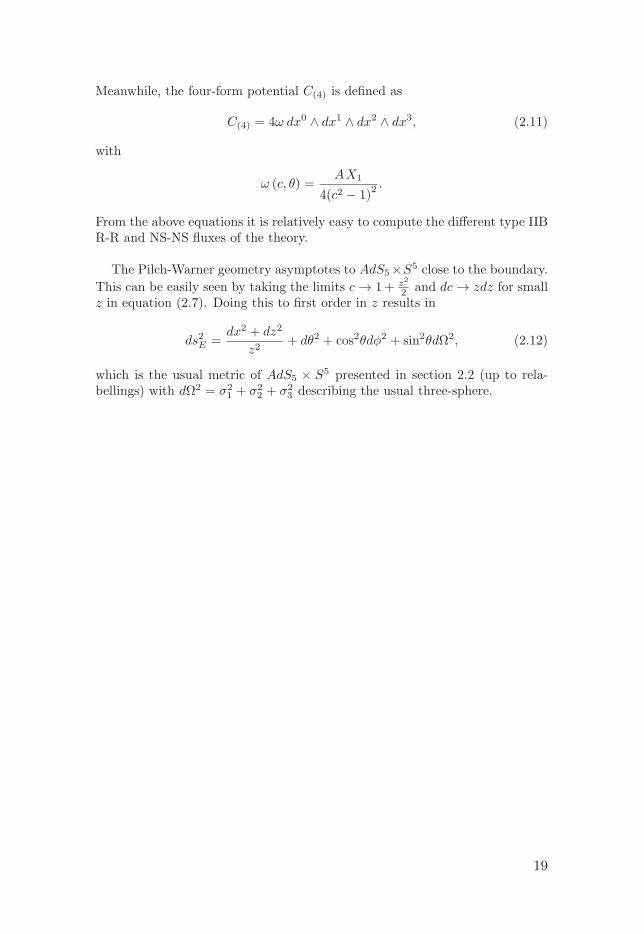
The Pilch-Warner geometry asymptotes to AdS5×S5 close to the boundary.

This can be easily seen by taking the limits c → 1+ z2

2 and dc → zdz for smallz in equation (2.7). Doing this to first order in z results in

ds2E =dx2 + dz2

z2+ dθ2 + cos2θdφ2 + sin2θdΩ2, (2.12)

which is the usual metric of AdS5 × S5 presented in section 2.2 (up to rela-bellings) with dΩ2 = σ2

1 + σ22 + σ2

3 describing the usual three-sphere.

19

3. Wilson loops in AdS/CFT

The concept of Wilson loop was originally introduced by K. Wilson in the1970’s in an attempt to better understand the problem of confinement in quan-tum chromodynamics (QCD) in a non-perturbative manner [20], a problemthat to this day is still unsolved and is one of the Millennium prize problems.Wilson loops are useful for the study of gauge field theories as these observ-ables contain information on the underlying theory and can also play the roleof order parameter in the study of confinement.

In the last decades Wilson loops have been commonly used in the study of theAdS/CFT duality as a clearer picture of Wilson loops appeared at both sides ofthe duality due to the D3-brane picture. The holographic dual of Wilson loopswas proposed in the works [21, 22]. In the string theory picture, the dual tothe Wilson loop is given by the partition function of a string embedded in AdSsuch that its worldsheet ends at the boundary on the contour described by thefield theory loop. In the strong coupling limit, the string theory calculation ofWilson loops corresponds to the study of minimal areas of classical strings inAdS5 × S5.

Having a holographic picture of these observables, it is in principle possibleto test the AdS/CFT duality by computing Wilson loop expectation valuesat both sides of the correspondence (see for instance [23]). Due to advancesfrom supersymmetric localization [2], expressions are known for several Wilsonloop configurations in supersymmetric theories at all orders in the coupling.The aim of the present thesis is to further expand these tests by doing thecorresponding string calculations beyond leading order.

It is also important to mention that interest in Wilson loops in AdS/CFTgoes beyond testing the duality as Wilson loops over light-like polygons areconjectured to be dual to scattering amplitudes [24, 25, 26]. This surprisingfeature allows for the possibility of transferring knowledge from Wilson loops tothe study of other observables. Study of hidden symmetries of Wilson loops isalso an active area of research as the AdS/CFT duality connects Wilson loopsin N = 4 SYM to integrable classical strings on AdS5 × S5. In this setup,progress has been made in studying Yangian symmetry at strong and weakcoupling [27, 28], as well as in the study of the master and bonus symmetries[29, 30].

In this chapter, we will introduce several important physical concepts rele-vant for the calculations of papers I and II. Section 3.1 presents a very briefintroduction to the AdS/CFT duality. In section 3.2 we review the conceptof Wilson loop in field theories and in particular for the case of N = 4 superYang-Mills. Later, in section 3.3 the string theory picture of the MaldacenaWilson loop is presented. Finally, in section 3.4 we introduce the Wilson loop

20

configurations studied in papers I and II, namely; the Wilson line, the circularWilson loop and the latitude Wilson loop.

3.1 The AdS/CFT dualityIn physics, dualities are of great value as they provide a bridge between a prioritotally different physical theories. By providing a link between two equivalentdescriptions, dualities increase our understanding of theories at a fundamentallevel. The gauge-string correspondence has several realizations, the AdS/CFTduality proposed by Maldacena is the classic example, but there are other du-alities connecting for instance AdS4 × CP 3 and ABJM [31], or N = 2∗ andstring theory in the Pilch-Warner background.

In its “strongest version” the AdS/CFT duality states the exact equivalenceof N = 4 super Yang-Mills with SU(N) gauge group and type IIB superstringtheory on AdS5 × S5. In the field theory side the parameters of the theoryare the rank of the gauge group N and the value of its coupling constant gYM.Meanwhile, on the string theory side the parameters of the theory are thestring coupling constant gs and the ratio L/

√α′ with L denoting the radius of

curvature of AdS5 × S5 and α′ being related to the string length squared [32].According to the AdS/CFT dictionary, the parameters of these two theoriesare connected by

λ = g2YMN =L4

α′2, g2YM = 4πgs, (3.1)

where we introduced the ’t Hooft coupling constant λ. For practical reasons itis difficult to test this duality for arbitrary values of these parameters, thus itis convenient for calculation purposes to take certain limits. Non-perturbativeresults in string theory are few, thus it is sometimes convenient to explore theweak coupling limit of string theory gs � 1 for fixed values of L/

√α′, which

physically amounts to considering classical strings. From the r.h.s. of (3.1)we see that this corresponds to the Yang-Mills coupling gYM being very small,and from the l.h.s. of (3.1) this would imply having λ/N to be small too. Thelater can be achieved by considering N → ∞ for a fixed value of λ, whichis referred to as the ’t Hooft limit. From the field theory side all non-planarFeynman diagrams vanish in this limit and consequently it is also called the“planar limit”. Thus, in this limit, classical strings in AdS5×S5 are dual to theplanar limit of N = 4 SYM: This is usually referred to as the “strong version”of the duality.

Having already taken the limits of N → ∞ and gs → 0, there are only twoarbitrary parameters left in the duality: λ in the N = 4 SYM side and L/

√α′

on the AdS5 × S5 side of the duality. As we mentioned in the introductionof chapter 1, quantum field theories at strong coupling concern some of themost challenging problems in theoretical physics, as perturbation theory breaksdown. Taking the strong coupling limit corresponds to doing λ → ∞ in thefield theory side and

√α′/L → 0 on the string theory side. Being L the radius

21

of curvature of AdS5×S5 and α′ being given by the square of the string length,√α′/L → 0 corresponds to considering strings of point-particle nature. The

later are described by type IIB supergravity in AdS5×S5. The duality betweensupergravity in AdS5×S5 and the N = 4 SYM in this planar and λ → ∞ limitis usually referred to as the “weak version” of the duality.

It is important to keep in mind the above limits as the aim of the present the-sis is to study Wilson loop perturbative computations in string theory, whichamounts to considering string theory in the limit gs → 0. In principle, dueto localization, the Wilson loop configurations studied here are understood forarbitrary values of λ in the field theory side. However, in the string theory sideonly the classical contributions are fully understood, being the semiclassicalcontributions the object of study of the present thesis.

A natural check of the duality concerns the symmetries on both sides. Asdiscussed in section 2.2, string theory in AdS5 × S5 has PSU(2, 2|4) symme-try. In the field theory side one has the same symmetry, though it emergesin a different way. N = 4 SYM is a conformal theory preserving N = 4 su-persymmetry: Supersymmetry in this case implies the existence of 16 Poincaresupercharges and conformal symmetry is responsible for an additional 16 super-charges, all of these symmetries form PSU(2, 2|4). Naturally, having the samesymmetry is not a sufficient condition for the two theories to be equivalent, butit is a necessary condition.

An additional feature of the correspondence is also the fact that it realizesthe holographic principle. The later is an idea in physics which states that theinformation contained in a d-dimensional volume is encoded in its d−1 bound-ary area. In the AdS/CFT duality the way to think about it is by consideringAdS5 as the “bulk” gravitational theory, while 4-dimensional N = 4 SYM livesat its “boundary”; being the two theories equivalent, all the information con-tained in the “bulk” of AdS is encoded in its lower dimensional gauge theorydual N = 4 SYM.

Finally, we conclude by mentioning that due to the ever increasing literatureon the topic, any review on the AdS/CFT duality falls short of presenting acomplete picture. However, it is worth mentioning that the duality has foundapplications in many areas of physics; providing new insights into relativistichydrodynamics [33, 34], the quark-gluon plasma [35], condensed matter sys-tems [36, 37, 38], etc. By offering the possibility of studying quantitativelystrongly coupled physical phenomena, the duality is a potential window tounderstanding physics that would be unaccessible by other methods.

3.2 Wilson loops in field theoryIn field theory, Wilson loops are operators describing the parallel transportof a very massive quark along a closed path C and physically correspond tothe phase factor acquired by the quark field in such process. For the case ofYang-Mills with SU(N) as gauge group, the formula describing the Wilson loop

22

operator in the fundamental representation is [32]

W (C) =1

Ntr P exp

[∮C

ds (iAμxμ)

], (3.2)

where Aμ(s) is the gauge field lying in the Lie algebra, xμ(s) is a parametriza-tion of C, P denotes path-ordering of the fields in terms of s, and the trace istaken over the fundamental representation. By definition W (C) is a non-localoperator and it is also gauge-invariant.

The expectation value of Wilson loop operators 〈W (C)〉, which is the phys-ical quantity we will be interested in, plays an important role as it gives infor-mation on the field theory in question. In principle, knowledge of all Wilsonloop configurations is sufficient for reconstructing the gauge potentials of thetheory [39]. For instance, the quark anti-quark potential can be written interms of the Wilson loop expectation value

V (R) = − limT→∞

1

Tln 〈W (C (R, T ))〉 ,

where the contour C is a rectangle of sides R and T , with R � T .

The Wilson loop operator for the case of N = 4 super Yang-Mills wasproposed by Maldacena and it is given by [21, 22]

W (C) =1

Ntr P exp

[∮C

ds(iAμx

μ + |x|Φini)]. (3.3)

Compared to (3.2) the Maldacena Wilson loop introduces an extra coupling inthe exponential, which depends on the scalar fields Φi of N = 4 SYM and ona unit-norm six-vector ni(s) that maps every point in C to a point in S5.

A priori such a formulation for Wilson loops in N = 4 super Yang-Mills isnon-trivial as this field theory has massless matter and transforms under theadjoint representation. To circumvent these issues the proposal in [21] startswith a SU(N + 1) N = 4 SYM field theory and introduces massive quarksby means of a breaking of symmetry SU(N + 1) → SU(N) × U(1) such thatthe corresponding W-bosons acquire a mass and transform in the fundamen-tal representation of SU(N). This breaking of symmetry from SU(N + 1) issuch that the scalars of this theory, which are valued in su(N + 1), break intothe massless scalars of su(N) plus fields transforming in the fundamental (andanti-fundamental) representation of su(N) which have mass due to the Higgsmechanism. The phase factor in the propagator of such fields in backgroundgauge and scalar fields is in fact the Maldacena Wilson loop [40].

3.3 Wilson loops in string theoryThe string theory dual of the Maldacena Wilson loop expectation value is givenby the partition function of a string whose worldsheet Σ ends on a contour C at

23

Figure 3.1. Holographic picture of a Wilson loop: The string worldsheet is inthe bulk of AdS and encloses C at the boundary.

the boundary of AdS, as seen in Figure 3.1. The superstring partition functionis given by [21]

〈W (C)〉 = Z =

∫DXμDΨDhij e−SString(h,X,Ψ),

where the integration is carried over the target space coordinates Xμ, thefermionic fields Ψ and the worldsheet metric hij .

At a glance it is easy to see that the expression above is not well defined asit has overcounting over physically equivalent configurations which are relatedby Weyl and diffeomorphism transformations. Therefore, in order to makesense of the path integral, it is necessary to do gauge-fixing. We first fix theworldsheet metric to be given by the metric induced by a classical solutionXcl

μ (τ, σ) ending at the required geometry in the boundary of AdS

hij = ∂iXclμ (τ, σ) Gμν (Xcl) ∂jXcl

ν (τ, σ) , (3.4)

where the classical string solution satisfies the boundary condition

Xclμ (τ, σ)|∂Σ = xμ (s) ,

with the r.h.s. being previously defined in section 3.2. In order for this gauge-fixing procedure to produce the correct measure of the path integral, it isnecessary to introduce the Faddeev-Popov ghosts. Additionally, it is also nec-essary to fix the fermionic κ-symmetry in order not to double count fermionicdegrees of freedom. There are many ways to fix the later, here we do as in[3, 9] and impose Ψ1 = Ψ2 = Ψ. These considerations result in

〈W (C)〉 = Z =

∫DXμDΨ e−SString(X,Ψ) det1/2P †P,

24

where the determinant on the right is due to the Faddeev-Popov procedure.

Following the semiclassical quantization procedure of [3] for the Green-Schwarz string, we expand the string embedding coordinates Xμ around theclassical solution Xμ

cl

Xμ = Xμcl + δXμ = Xμ

cl + Eaμξa, (3.5)

where δXμ denote quantum fluctuations around the classical solution and ξa

their corresponding projection into tangent space. The later will be the defaultbasis in which to consider bosonic fluctuations since fermions are only definedin the tangent space and, due to supersymmetry, both path integrals shouldbe treated in a similar manner.

By expanding the bosonic Lagrangian density (2.1) up to second orderin fluctuations and integrating by parts, one finds the structure LB (X) =LB (Xcl)+ ξKBξ where linear terms in ξ vanish due to the equations of motionand KB denotes second order differential operators. Meanwhile, the expansionin fluctuations for the fermionic piece (2.4) results in LF (X,Ψ) = ΨKFΨ withKF denoting differential operators linear in derivatives. By replacing in thepath integral it is easy to see that both fermionic and bosonic integrals are ofGaussian type, thus obtaining

〈W (C)〉 = Z = e−SString(Xcl)det1/2KF

det1/2 KB

det1/2P †P. (3.6)

The expression above for the string partition function is composed of two pieces,each one with a different functional dependence on λ. We now present the mainfeatures of each.

3.3.1 The classical action

The contribution coming from the classical action SString(Xcl) is obtained byevaluating equations (2.1) and (2.2) at the classical solution. Physically, thiscontribution corresponds to the leading term of the Wilson loop expectationvalue at strong coupling (λ 1) and its dependence on the ’t Hooft couplingis of the form SString(Xcl) =

√λ Const. In the literature, such classical contri-

butions are well understood and in general agree with field theory predictions.For the case of the AdS5 × S5 background, classical contributions have a

nice geometrical interpretation. Due to the absence of B-field and dilaton, theonly non-vanishing contribution comes from the Polyakov action evaluated atthe classical solution. The later is understood to have the following structure

〈W (C)〉 λ�1= exp

[−√λ

2πAren (C)

],

where Aren denotes the “renormalized” area of the worldsheet. In principle,direct evaluation of the Polyakov string at the classical solution results in adivergent result. The reason for this divergence resides in the existence of the

25

1/z2 singularity of the metric tensor at the boundary. The way to regularize thisdivergence is by considering the integration volume to start from a small cutoffz = ε close to the boundary. The regularization procedure can be summarizedby considering

Aren (C) = limε→0

[A (C)|z�ε −

L

ε

],

where L denotes the perimeter around C. Another way to think about the reg-ularization procedure is by implementing the Legendre transform of Z, whichamounts to dropping the 1/ε divergences in the final result [40].

It is important to keep in mind that for more complicated supergravity back-grounds with non-trivial dilaton, like the Pilch-Warner background, one has anadditional contribution coming from the Fradkin-Tseytlin term. This contri-bution is classical in nature and will play an important role in the calculationsof paper I.

3.3.2 The semiclassical partition function

Contributions to the semiclassical partition function come from the evaluationof the functional determinants in (3.6) and will be the focus of the presentthesis.

In principle, provided that the functional determinants considered do nothave zero modes, the semiclassical partition function would have a dependenceon λ of the form λ0. If the spectrum in one of the determinants has zero modes,each would contribute with a factor λ−1/4 to the determinant. The later canbe seen more clearly through the use of collective coordinates when evaluatingthe determinants [41].

Before proceeding, we will briefly present some features of the individual con-tributions to the semiclassical partition function. The fermionic contributioncomes from fixing κ-symmetry and evaluating the terms in between Ψ and Ψ in(2.4) at the classical solution. In principle, being Ψ a 16-component spinor, theresulting differential operator will be a 16×16 matrix. The later can be usuallyreduced to much simpler 2× 2 blocks by choosing a convenient representationof Dirac matrices. Naturally, the choice of gauge and Dirac matrices does notchange the physics of the problem, but the expressions involved become muchsimpler. The resulting differential operators KF will be linear in derivativeswith respect to τ and σ. Since it is customary (although not necessary) toconsider determinants of operators of a Laplace type −∇μ∇μ, the fermionicoperators in KF are sometimes squared and one studies the determinant of thelater [42].

The bosonic contribution comes from expanding the ten coordinates in (2.1)around the classical solution. Depending on the field content involved, it issometimes convenient to use the following expression from which one can readthe differential operators after partial integration and projecting the fluctua-

26

tions to tangent space [43]

L(2)B =

1

2

√h[Gμν (Xcl)Diξ

μDiξν +Rμναβ (∂iXμcl)(∂iXβ

cl

)ξνξα

−1

2(∂iX

αcl)(∂jX

βcl

)εijξμξν∇μHναβ +

1

4(∂iX

νcl)(∂iXβ

cl

)HμναH

αβλξ

μξλ],

where εij is the Levi-Civita tensor, ∇ is the covariant derivative, hij wasdefined in equation (3.4) and

Diξμ = ∂iξ

μ + Γμνα (Xcl) (∂iX

αcl) ξ

ν +1

2εi

j (∂jXνcl)H

μναξ

α.

When evaluating the functional determinants it is important to remember thateach spectral problem corresponds to a differential operator, a set of boundaryconditions and an inner product. The inner product is important in the evalu-ation of the functional determinants as the later should only have contributionsfrom normalizable fluctuations. The norm of fluctuations (in tangent space) isgiven by the inner product⟨

ξa, ξb⟩=

∫∫ √h ξaξbdτdσ.

The Faddeev-Popov determinant results from the Gaussian integration ofthe ghost action. The later is of the form [3, 44]

LFP =1

2

√hhij

(∇kεi∇kεj − R(2)

2εiεj

).

After projecting on the worldsheet tangent space using the worldsheet veilbein

(εi = eijεj) and integrating by parts, it can be shown that the resulting opera-

tor is the same as the bosonic differential operator along directions longitudinalto the string worldsheet.

The fact that the ghost and bosonic longitudinal modes result in the samedifferential operator does not imply that the resulting determinants are thesame and that their contributions cancel. The reason for this is that the spec-trum also depends on the boundary conditions imposed, and the later are notthe same for ghosts and bosonic longitudinal modes [3]. The difference in thespectrum of ghosts and longitudinal modes is sometimes attributed for themismatch in semiclassical string partition function calculations. In particular,presence of zero modes in one of the operators is commonly assumed to beresponsible for lnλ terms when evaluating ln 〈W (C)〉 [23].

In order to avoid these ambiguities we evaluate the ratio of two Wilson loopswith the same geometry in paper II, where the corresponding contributions areexpected to cancel between latitude and circular Wilson loops. Meanwhile, forthe case of the straight line the ratio of ghost and longitudinal mode deter-minants is assumed to cancel. This is motivated by the fact that ghost zeromodes are not normalizable in this case and that similar ghost/longitudinalmode cancelations have lead to correct results in string theory [9, 45]. Thus,from now on when mentioning bosonic operators we refer exclusively to those

27

along the eight directions transversal to the string worldsheet.

From the considerations above, the quantity that we will study is

〈W (C)〉 = Z = e−SString(Xcl)det1/2KF

det1/2 KB

. (3.7)

In order to evaluate the determinants, we will impose Dirichlet boundary con-ditions at the boundary of AdS. In principle, an eigenfunction of a second orderdifferential operator is given by the superposition of two solutions. In our pro-cedure we choose those solutions that vanish at the boundary and are wellbehaved in its neighbourhood. Due to the 2× 2 nature of fermionic operators,it is often the case that one component vanishes while the other does not atthe boundary. For this fermionic cases we choose the superposition which isfinite approaching the boundary, as usually one of them diverges. More detailson the boundary conditions imposed are presented in chapters 5 and 6. Thetechnique used to evaluate the corresponding determinants is introduced laterin chapter 4.

3.4 Loop configurationsWe now present the Wilson loop configurations considered in papers I and II.Their geometry and localization predictions are shown for each case, and wecomment on the state of the corresponding string theory calculations.

3.4.1 The Wilson line

This Wilson loop operator corresponds to an infinite straight line with a contourparametrized by xμ(s) = (s, 0, 0, 0). When the field theory considered is N = 4SYM the result is

〈W (C)〉line = 1. (3.8)

The above result is a consequence of the Wilson loop operator commuting withhalf of the 16 supercharges, making it BPS, and thus being protected fromquantum corrections [8]. From the holographic perspective, this is perhaps thebest understood configuration as the classical and semiclassical string parti-tion functions in AdS5 × S5 have been shown to reproduce the field theoryresult using several methods for the evaluation of determinants [3, 7, 9]. Thecorresponding classical string solution is given by

zcl = σ, x0cl = τ, (3.9)

while other coordinates vanish such that the classical string describes an in-finitely long line in AdS with σ ∈ [0,∞) and τ ∈ [0, 2π].

28

The Wilson line was considered in [6] for the case of N = 2∗ obtaining thefollowing field theory prediction at strong coupling

ln 〈W (C)〉line = ML

[√λ

2π− 1

2+O

(1√λ

)], (3.10)

where M is the mass parameter and L is the length of C. In [46] the first term onthe r.h.s. was successfully matched with the classical string partition functionof the Pilch-Warner background. Obtaining the λ0 term in string theory is themain result of paper I. In the process, we also reproduced the result (3.8) in asimple and elegant manner. The classical string solution for the Pilch-Warnerbackground has naturally the same geometry and is parametrized by ccl = σand x0

cl = τ in the coordinates of section 2.3.

3.4.2 The circular Wilson loop

The circular Wilson loop operator is 1/2 BPS and its parametrization is givenby

xμ (s) = (cos s, sin s, 0, 0) , ni (s) = (0, 0, 1, 0, 0, 0) .

In the field theory side, in N = 4 SYM the expectation value for this operatorwas conjectured to be described by a Gaussian matrix model in [8, 23] andits result was proven using supersymmetric localization in [2]. The expectationvalue for this Wilson loop is known for all values of the rank of the gauge group(N) and all values of λ. In the planar limit the result is

〈W (C)〉circle =2√λI1

(√λ), (3.11)

which has the following behaviour at strong coupling

ln 〈W (C)〉circle =√λ− 3

4lnλ− 1

2ln

π

2+O

(1√λ

). (3.12)

In the string theory side, this Wilson loop is described by the following classicalsolution describing a circle in the boundary of AdS

xμcl =

(cos τ

coshσ,sin τ

coshσ, 0, 0

), zcl = tanhσ, ψcl = 0, ϕcl = any,

while the angles φi with i ∈ {1, 2, 3} are arbitrary constants. In the expressionabove σ ∈ [0,∞) and τ ∈ [0, 2π].

The string theory computation of (3.12) in AdS5 × S5 has only been suc-cessful at leading order in λ. The first term in equation (3.12) is reproduced byconsidering the string action evaluated at the classical solution. The lnλ termhas been conjectured to be produced by the normalization of ghost zero-modesin the partition function. Meanwhile, the remaining term in (3.12) is under-stood to come from fluctuations around the classical solution. Despite several

29

attempts [7, 9, 10], exact matching of (3.12) with string theory calculations hasnot been achieved for the last term, while the lnλ term has not been properlyexplained.

This Wilson loop can also be studied in the case when it has a winding k,in which case the equations (3.11) and (3.12) are valid after the substitutionλ → k2λ. The dependence on k is also a mystery from the string theory sideas calculations based on Gel’fand-Yaglom [9] and heat kernel methods [11, 14]have lead to discrepancies with localization results.

3.4.3 The latitude Wilson loop

The latitudeWilson loop operator describes a family of Wilson loops parametrizedby an angle θ0 describing a latitude in a S2 ⊂ S5 and finishing in a circle atthe boundary of AdS. The operator is 1/4 BPS and is parametrized by

xμ (s) = (cos s, sin s, 0, 0) , ni (s) = (sin θ0 cos s, sin θ0 sin s, cos θ0, 0, 0, 0) .

It is easy to see that the above Wilson loop in N = 4 SYM reduces to the1/2 BPS circular Wilson loop described in section 3.4.2 when θ0 = 0, while forθ0 = π/2 it corresponds to the Wilson loop studied in [47]. The predictionsfrom localization for its expectation value are obtained through the substitutionλ → λ cos2θ0 resulting in [48]

〈W (C)〉latitude =2√

λ cos θ0I1

(√λ cos θ0

)in the large N limit and

ln 〈W (C)〉latitude =√λ− 3

4lnλ− 3

2ln cos θ0 − 1

2ln

π

2+O

(1√λ

)at strong coupling.

The corresponding classical string solution describes a circle in the boundaryof AdS and extends into an S2 ⊂ S5

xμcl =

(cos τ

coshσ,sin τ

coshσ, 0, 0

), zcl = tanhσ,

cosψcl = tanh (σ + σ0) , ϕcl = τ, (3.13)

where τ ∈ [0, 2π], {σ, σ0} ∈ [0,∞) and σ0 is written in terms of θ0 as

tanhσ0 = cos θ0.

The string theory computation of this Wilson loop has not been consideredindependently as the particular case θ0 = 0 is already problematic. Instead,efforts have been done on studying the ratio between the semiclassical partitionfunctions of a latitude with arbitrary angle θ0 and the case θ0 = 0 (which wasdescribed in section 3.4.2). The hope is that since both worldsheets have thesame topology, measure factors and possible ghost contributions would cancel.

30

This ratio of Wilson loops is understood at leading order in λ in terms ofthe classical actions [48]. However, computations of the semiclassical stringpartition function in AdS5×S5 led to discrepancies with the localization resultwhen the determinants were evaluated using the Gel’fand-Yaglom method [12,13]. Agreement was reached at first order in perturbation theory for very smallθ0 using a series expansion of the heat kernel [14], and more recently using zetafunction regularization [15]. In paper II perfect agreement was reached withthe localization prediction for this ratio at all orders in θ0.

31

4. Functional determinants

As we discussed in the previous chapter, in the framework of the gauge-stringduality, the string theory computation of Wilson loops consists in the eval-uation of a string partition function around a classical string configuration.At first order at strong coupling, contributions come from the minimal areadescribed by the string worldsheet. Meanwhile, computation of 1-loop cor-rections to the string partition function reduces to the problem of evaluatingdeterminants of several differential operators. The later is a highly non-trivialtask as determinants of differential operators themselves are usually divergentquantities.

Evaluation of determinants of differential operators plays an important rolein theoretical physics, as it is a technique appearing extensively in many areasof physics and mathematics. Motivation to study such techniques in physicscomes for example from the study of effective actions appearing in relativisticand non-relativistic many-body physics, tunnelling and nucleation processes[49, 50], lattice gauge theories, gauge fixing and Faddeev-Popov determinants,evaluation of entanglement entropy, etc. Despite the widespread appearance offunctional determinants in mathematical physics, exact results are only knownfor few cases like the Klein-Gordon or Dirac operators on spheres or tori. Fordifferential operators on arbitrary backgrounds the picture is not so clear andat times one has to rely heavily on approximation methods.

Historically, the recurrent appearance of differential operators in theoreticalphysics came partly due to the appearance of Quantum Mechanics [42]. Later,it became known that the spectrum of such operators can be described in termsof spectral functions, the most commonly used being the heat kernel. Thismethod played an important role in the understanding of quantum correctionsdue to the work of DeWitt in the 1960’s [43]. Later, it was realized thatinformation on the spectrum of differential operators could be encompassedin terms of the zeta function of the operator. More sophisticated techniqueslike the Gel’fand-Yaglom method [51] have received widespread use, as theyallow for the computation of functional determinants without requiring fullknowledge of the eigenfunctions in question.

In this chapter we will briefly discuss the main features of some of thesemethods in section 4.1. In section 4.2, based on the previous section, we reviewsome results for the contribution of conformal factors to functional determi-nants relevant for the calculation in paper II. Section 4.3 presents identitieswhich will simplify the calculation in paper I. Then in section 4.4 we motivatethe method based on the scattering phaseshifts, which will be used later forthe calculation of 1-loop string corrections of Wilson loops in papers I and II.

32

4.1 Zeta function & heat kernelDue to the large amount of literature on the subject, we only present the mainfeatures of these techniques which will be useful later in section 4.2. Heat ker-nel and zeta function techniques will not be explicitly used in this thesis for theevaluation of determinants. However, identities from these approaches will beuseful in the calculation of paper II for a check on the underlying assumptions.The presentation of the topic in this section is largely based on [42, 43] withmany details deliberately swept under the rug.

Let K be a self-adjoint second order differential operator, its determinantcan be written in the form

ln detK = −ζ ′ (0;K) , (4.1)

where ζ(s;K) is the zeta function of K. The later is usually defined in termsof the eigenvalues λ of K through

ζ (s;K) =∑λ

λ−s, (4.2)

where we assume that λ ∈ R and λ > 0.From the equation above, explicit knowledge of all eigenvalues λ would in

principle lead to the calculation of the determinant. However, it is not im-mediate that this series converges as for large values of λ the r.h.s. of (4.2)converges if Re s > n/2 where n denotes the dimensionality of the manifold(n = 2 in our case as the string worldsheet is 2 dimensional). Analytic exten-sion of the zeta function can be done for values of s in the rest of the complexplane. Moreover, this expression can also be extended to operators with nega-tive eigenvalues and Dirac type operators. These extensions will not be used inour work as our calculations do not rely on the zeta function method, howeverzeta function methods have recently been used in the study of latitude andcircular Wilson loops in [15] and [52].

One of the main advantages of the zeta function method is its simplicityand the fact that it is easily connected to other methods for evaluation ofdeterminants, in particular the heat kernel method. The later is a widely usedmethod based on knowledge of a function K(x, y|t) satisfying

(∂t +Kx)K (x, y|t) = 0, K (x, y|0) = δ(n) (x− y) , (4.3)

where K(x, y|t) is usually referred to as the “heat kernel”. Despite the relativesimplicity of (4.3), the heat kernel is only known for few Laplace and Diracoperators in very symmetric manifolds like the sphere or flat-space. For morecomplicated geometries, like that of the Pilch-Warner or the latitude Wilsonloop, the corresponding heat kernel is not known.

The heat kernel of the operator K can be written in the form

K (x, y|t) = 〈x| e−tK |y〉 , (4.4)

33

and tracing over x and y leads to

K (K; t) = K (1,K; t) =

∫ √h K (x, x|t) dxn

=∑λ

e−tλ, (4.5)

where in the first line we used the definition of the “heat trace”

K (f,K; t) = Tr[f e−tK] (4.6)

evaluated for a “smoothing function” f = 1. Meanwhile, the second line of(4.5) is a consequence of taking the trace of (4.4).

The bridge between the heat kernel and zeta function methods is made bythe equation

ζ (s;K) =1

Γ (s)

∞∫0

ts−1K (K; t) dt, (4.7)

which is a direct consequence of (4.2) and the second line of (4.5). Equation(4.7) connects the heat trace of the operator K with its zeta function, making itpossible to calculate detK provided one knows the heat kernel K(x, y|t). Thedeterminant of K can be written in terms of the heat trace as

ln detK = − lims→0

d

ds

1

Γ (s)

∞∫0

ts−1Tr e−tKdt. (4.8)

We conclude our presentation of the heat kernel method by introducing the“heat kernel coefficients” which are the coefficients ap in a series expansion ofthe heat trace for t → 0

K (f,K; t) =

∞∑p=0

ap (f,K) t(p−n)/2. (4.9)

The heat kernel coefficients are very useful as they depend on informationon the operator, the manifold and the boundary conditions, and can provideinformation on the functional determinants as will be shown in section 4.2.Depending on the imposed boundary conditions, an expression for the heatcoefficients may or may not be known in the literature. For later use, wepresent the coefficient a2(f,K) for Dirichlet boundary conditions

a2 (f,K) =1

(4π)n/2

⎡⎣∫M

√h Tr

(f

(R

6− E

))dxn

+

∫∂M

√g Tr

(f

3Kj

j − 1

2∇nf

)dxn−1

⎤⎦ , (4.10)

34

where Kij is the extrinsic curvature at the boundary, gij is the metric at the

boundary, ∇n the covariant derivative projected along the direction normal tothe boundary and E comes from writing the operator in “covariant form”

K = −hijDiDj + E, (4.11)

whereDi can have Riemann and gauge connections parts. When the operator ofinterest is linear in derivatives, as is usually the case for fermions, one considersthe square of the operator.

Several identities presented in this section for the heat kernel will be usefulfor a check on the assumptions of paper II. This check is based on the machinerydeveloped in the next section.

Before finishing our discussion on the main features of the heat kernelmethod, we discuss their role in string theory Wilson loop computations. De-spite the fact that the heat kernel method can not be used for the straightline computation of paper I due to ignorance on the heat kernel for the Pilch-Warner geometry, heat kernel computations of the straight line in AdS5 × S5

have successfully reproduced the field theory prediction [7].The heat kernels needed for the 1/2 BPS circular Wilson loop computation

are known [53, 54, 55, 56], but there is a mismatch with the field theory pre-diction [7]. For the case of the latitude Wilson loop studied in paper II, noexpression is know for the heat kernel, however, a perturbative result startingfrom the known heat kernel of the case θ0 = 0 led to reproducing the local-ization result at first order in perturbation theory of the ratio of circular andlatitude loops [14].

Using the heat kernel of the circular Wilson loop and the Sommerfeld for-mula, the case of the k-winding circular Wilson loop was studied in [11], leadingto a mismatch with field theory predictions. In spite of the vast mathematicalliterature on this method, its applications for the string theory calculation ofWilson loops seem rather behind.

4.2 Determinants & conformal factorsThe operators considered in paper II have a factor depending on σ in front ofthe ∂2

τ and ∂2σ derivatives. The method we use to evaluate determinants, which

will be introduced in section 4.4, requires this factor to be −1. The dependenceof determinants in terms of these factors is given through the Seeley coefficientsintroduced in the previous section. We will first show how the dependence onthe conformal factors is encoded in the heat kernel coefficients and then we willderive concrete expressions for bosonic and fermionic operators.

The bosonic operators of interest can all be written in the canonical form

K(α) = e 2αφ(−δijDiDj + E

), (4.12)

where α ∈ [0, 1] is a constant, φ is a scalar function depending on the worldsheetcoordinates, the derivative can have a “gauge” part Dj = ∂j + iAj , while Aj

and E are n× n matrices which can depend on both τ and σ.

35

On the other hand, the fermionic operators of interest in paper II are 2× 2Dirac operators of the form

D(α) = e3αφ2

(iγjDj + γ3a+ 1v

)e−

αφ2 , (4.13)

where the contraction is done with the Euclidean metric, a and v are scalarfunctions depending on the worldsheet coordinates, while Dj = ∂j + iAj withAj a 2×2 matrix that can depend on {τ, σ} and is proportional to the identitymatrix. Just as for bosons α ∈ [0, 1] is a constant parameter and φ is a scalarfunction depending on worldsheet coordinates. To make direct comparison withthe fermionic operators of paper II, it is convenient to use the following basis

γτ = −τ2, γσ = τ1, γ3 ≡ −iεμνγμγν/2 = τ3.

We are interested in how the determinants of the operators (4.12) and (4.13)change when the parameter α takes the values α = 0 and α = 1. When α = 1we will recover the operators obtained from the Green-Schwarz action, whileα = 0 produces the operators for which we will calculate the determinantswith the phaseshift method. The dependence of the determinants on α can beexplicitly shown using expressions from section 4.1 and following the argumentsin [3].

From equation (4.12) it is easy to see that

∂

∂αTr e−tK = 2t

∂

∂tTrφ e−tK. (4.14)

Differentiating (4.8) with respect to α and replacing the expression above re-sults in

d

dαln detK = 2 lim

s→0

d

ds

s

Γ(s)

∫ ∞

0

dt ts−1 Trφ e−tK. (4.15)

The integrand above can be badly behaved around t = 0. To perform thisintegral we use the expressions (4.6) and (4.9) for the heat trace, as well as theidentity ∫ ∞

0

dt tsf(t)s→0=

1

srest=0

f(t) + regular.

Doing so results ind

dαln detK = 2a2(φ|K). (4.16)

In summary, the dependence of functional determinants on the conformal fac-tor is through the DeWitt-Seeley coefficient a2.

Using equations (4.10) and (4.11), it can be shown that the DeWitt-Seeleycoefficient for the bosonic operator defined in (4.12) is

a2 (φ,K) =1

4π

∫dσ2

(αn3φδij∂i∂jφ− φ TrE

)+

n

24π

∮ds (2αφ∂nφ− 3∂nφ).

Integrating with respect to α we finally obtain

lndetK(1)

detK(0)=

1

2π

∫d2σ

(n6φδij∂i∂jφ− φTrE

)+

n

12π

∮ds (φ∂nφ− 3∂nφ) .

(4.17)

36

To compute how the determinant of the fermionic operator in (4.13) dependson the conformal factor, we must first bring it to the canonical form (4.11) bysquaring, which results in

D2(α) = e 2αφ[−∇i∇i +

α

2∂i∂

iφ+ a2 − v2

+ εij (∂ia+ αa∂iφ) γj +

(1

2εijFij + 2av

)γ3

], (4.18)

where contractions are done with the Euclidean metric δij and

∇j = Dj − ivγj − iα

2εjk∂kφγ

3. (4.19)

Following the same arguments used for bosons, it can be shown that for thefermionic operator

d

dαln detD2 = 2a2(φ|D2). (4.20)

By explicit computation using equations (4.10) and (4.18), the DeWitt-Seeleycoefficient for the fermionic operator results in

a2(φ,D2

)= − 1

2π

∫dσ2

(α6φδij∂i∂jφ+ φ

(a2 − v2

))+

1

12π

∮ds (2αφ∂nφ− 3∂nφ).

Integration over α results in the final expression for fermions

1

2ln

detD2(0)

detD2(1)=

1

2π

∫d2σ

[1

12φδij∂i∂jφ+ φ

(a2 − v2

)]− 1

12π

∮ds (φ∂nφ− 3∂nφ) . (4.21)

Equations (4.17) and (4.21) will play an important role in the computationof paper II as they give us information on how the determinants are affectedby this conformal factor, which needs to be removed in order to evaluate thedeterminants.

4.3 Isospectral operatorsDepending on the operators being studied, it is sometimes possible to makestatements on the spectrum of two operators without having to explicitly cal-culate all the set of eigenvectors and eigenvalues. Take for instance the secondorder differential operators given by

KI = L†L, KII = LL†, (4.22)

where L and L† denote operators linear in derivatives. By simple algebra it iseasy to see that

KIL† = L†KII, KIIL = LKI.

37

These relations, also called “intertwining relations” allow to map the spectrumof one operator into another. Let us consider ψI and ψII eigenfunctions of KI

and KII satisfying

KIψI = ΛIψI, KIIψII = ΛIIψII. (4.23)

It is easy to see to check that

KI

(L†ψII

)=

(KIL†)ψII = L†KIIψII = ΛII

(L†ψII

),

KII (LψI) = (KIIL)ψI = (LKI)ψI = ΛI (LψI) .

Thus, L†ψII is an eigenvalue of KI and LψI is an eigenvalue of KII. In this way,one can map the eigenvalues and eigenvectors of one operator into the other.Operators of the type (4.22) are commonly called “isospectral” operators asthe spectrum of the two can be identified up to zero modes.

In principle, when considering the evaluation of determinants it is not suf-ficient for the operators to be isospectral in order for their determinants to bethe same. To see this more clearly one may think of the eigenfunctions ψI andψII as each being a superposition of two solutions to the spectral problems in(4.23). In order for the eigenvalues of ψI and ψII to contribute to the determi-nants of KI and KII, the eigenfunctions must satisfy the boundary conditionsof the problem. Imposing boundary conditions fixes the coefficients in the su-perpositions of ψI and ψII. If the choice of boundary conditions is compatiblewith the map

ψI ∝ L†ψII, ψII ∝ LψI.

then it is possible to identify the eigenfunctions contributing to the two deter-minants and the later will be the same.

Operators of this type are commonly seen in supersymmetric quantum me-chanics. Due to the underlying supersymmetry of string theory it is not entirelysurprising to find that some of the operators appearing in semiclassical stringpartition functions share this property. The later is the case for a fraction ofthe operators appearing in the computation in paper I which will simplify thecalculations considerably.

4.4 Phaseshifts & determinantsThe method we will use to evaluate the functional determinants in papers Iand II relies on explicit calculation of the eigenfunctions and eigenvalues of thedifferential operators. The operators we are interested in can be reduced afterFourier expansion in the τ coordinate into 1-dimensional operators of the form

K = −∂2σ + V (σ) , (4.24)

with the following asymptotic behaviour

K∞ = limσ→∞K = −∂2

σ + V∞, (4.25)

38

where V∞ = V (∞) is a constant.The spectrum of this type of operators can be qualitatively divided in

three parts. The first one consist on a continuum of exponentially increas-ing/decreasing functions. The second is a continuos spectrum of oscillatingfunctions. The third is composed by a finite number of discrete bound states.Naturally, to evaluate functional determinants it is necessary to choose a setof boundary conditions and an inner product. In principle, the determinantmust only receive contributions of eigenfunctions that satisfy both the bound-ary conditions and that have a finite norm.In flat space, exponentially increasing functions, and in most cases boundstates, will not have a finite norm. Meanwhile, the boundary conditions weare interested in consist of Dirichlet boundary conditions at the origin1

ψ(σ = 0) = 0. (4.26)

This type of boundary condition excludes exponentially decreasing functionsand some of the discrete parts of the spectrum. Thus, we are left with oscillatingfunctions and a finite number of discrete eigenfunctions contributing to thedeterminant.

As discussed previously, evaluation of determinants of elliptic differentialoperators usually results in divergences. The reason for this is that the deter-minant in question consists of an infinite product of eigenvalues. Consequently,one needs a regularization prescription. One option, as for instance done in thezeta function formalism of section 4.1, consists in removing the divergent piecesin such a way that only the physically meaningful finite piece remains. Anotherpossibility, which is the one we will use, consists on considering the ratio of twodeterminants instead of evaluating individual determinants. The justificationfor this resides in the fact that in many cases the divergent pieces cancel eachother, obtaining a finite result.

An ideal differential operator to use as a regulator in the ratio is the corre-sponding asymptotic operator K∞. Given the asymptotic differential operator(4.25), it is easy to see that the spectral problem

K∞ψ∞ =(−∂2

σ + V∞)ψ∞ = E∞(p) ψ∞

has for solutions plane waves of wave number p. After imposing the boundarycondition at the origin, the asymptotic eigenfunctions are of the form

ψ∞ ∝ sin (pσ) ,

with eigenvalue

E∞ (p) = p2 + V∞.

Meanwhile, the original spectral problem

K ψ =(−∂2

σ + V (σ))ψ = E(p) ψ (4.27)

1In paper I, the coordinates are such that σ ∈ [1,∞). Consequently, the boundarycondition used is ψ(σ = 1) = 0.

39

can be seen as a Schrodinger problem with potential V (σ). Depending on thepotential V (σ), analytic solutions for ψ(σ) may be found as in paper II or onemay need to resort to numerics as in paper I. In any case, since K limits to K∞for large σ, the eigenfunctions ψ(σ) will behave as plane waves asymptotically

limσ→∞ψ(σ) ∝ sin (pσ + δ(p)) ,

where δ(p) is a phaseshift generated by the potential.Physically, one can think of the continuum spectrum of K as consisting of

plane waves coming from infinity and interacting with the potential close tothe origin. This scattering of the incident wave with the potential will producea shift depending on the momentum p of the incident wave.

To evaluate the determinant we put the system in a box, which introducesan IR regulator R that corresponds to the length of the box. At a very largeσ = R we impose the quantization condition on the scattering states

pR+ δ(p) = πn,

which basically amounts to ψ (R) = 0. This quantization condition implies adensity of states

ρ(p) =dn

dp=

δ′(p)π

+R

π.

Meanwhile, for the asymptotic operator, for which there is no scattering, thequantization condition is

pR = πn, ρ∞(p) =dn

dp=

R

π, (4.28)

due to the absence of the potential.In terms of the densities of states we have that

lndetKdetK∞ =

∑n

EBSn +

∞∫0

ln(p2 + V∞

)δ′(p)π

dp, (4.29)

where the sum is over the discrete eigenvalues of K and the integration isover the ratio of continuum of states. This equation will be used later on forevaluating the different determinants considered in papers I and II.

As we mentioned earlier, the spectral problems we will consider can be re-duced to one dimension by Fourier expanding in the worldsheet direction τ .Consequently, for the problems of interest the r.h.s. of (4.29) will have sum-mation/integration over Fourier frequencies.

Naturally, since we will consider the superstring, operators of Dirac type willenter in the calculations of papers I and II. Operators of this type are not of theform (4.24), but we can square its eigenvalues and use (4.29). The reason whythis works is that for the 2 × 2 Dirac operators considered, decoupling of thecomponents leads to spectral problems of the type (4.27) for each component.Since the components are coupled, it is not always possible to impose (4.26)to both components. Instead, we will impose this condition to only one of thecomponents picking the better behaved solution at the origin. We will discussthis in more detail when doing the calculations of chapters 5 and 6.

40

5. Wilson line in the Pilch-Warner background

In this section we compute the semiclassical string partition function for thestraight line in the Pilch-Warner background which is the main result of paperI. As we discussed in section 3.4, this configuration is dual to the Wilson lineof N = 2∗ and its prediction from localization at strong coupling is

ln 〈W (C)〉line = ML

[√λ

2π− 1

2+O

(1√λ

)]. (5.1)

Here we calculate this quantity from the string side of the gauge-string corre-spondence based on the concepts introduced in chapters 2, 3 and the techniquespresented in chapter 4. For convenience we set M = 1, dependence on this vari-able can be easily recovered by dimensional analysis.

The string theory dual to the Wilson line in N = 2∗ is given by the classicalstring solution

x1cl = τ, ccl = σ, (5.2)

with τ ∈ [−L/2,L/2] and σ ∈ [1,∞), while all other fields are set to zero. Fromthe gauge fixing procedure discussed in section 3.3, the worldsheet metric takesthe value of the induced metric (3.4) resulting in

ds2w.s. =A

σ2 − 1dτ2 +

1

A(σ2 − 1)2 dσ

2, (5.3)

where now A ≡ A (σ).

Using the field content presented in section 2.3, we proceed in sections 5.1and 5.2 to compute the classical and semiclassical pieces entering equation (3.7).Later, in section 5.3 we discuss several aspects concerning the evaluation of thefunctional determinants. Finally, in section 5.4 we discuss the end result, as wellas the numerical setup needed for its calculation. To keep the presentation briefseveral technical details are omitted here, the reader interested in technicalitiesis referred to the original work in paper I.

5.1 The classical partition functionComputation of the contribution coming from the classical partition functionfollows from our discussion in section 3.3.1

SB (Xcl) =

√λ

2π

∫reg

dτdσ

(σ2 − 1)3/2

= −√λ

2πL, (5.4)

41

where integration over τ was performed in the interval −L/2 to L/2, while forσ the interval was from 1 + ε2/2 to infinity. The later is a consequence of thecoordinate c from Pilch-Warner being related to the holographic coordinate ofAdS by c → 1 + z2/2 for small z and the cutoff ε being located at z = ε. Asdiscussed in section 3.3.1, we use the regularization prescription of removingthe 1/ε divergences in the final result. From combining (3.7) and (5.4), we seethat the result above reproduces the localization prediction (5.1) at order λ1/2.

Since the Pilch-Warner background has a non-trivial dilaton, there is a con-tribution from the Fradkin-Tseytlin term presented in equations (2.2) and (2.3).Evaluation of this term at the classical solution results in

SFT (Xcl) =L

2π

∞∫1

dσ

σ√σ2 − 1

=L

4. (5.5)

Comparison of this result with the localization prediction (5.1) shows that thisterm corresponds to half of the λ0 final result. The other half results fromthe evaluation of quantum fluctuations around the classical solution and theirrespective determinants.

Writing both contributions together, we obtain the following result for theclassical piece of the partition function

SString (Xcl) = −L

(√λ

2π− 1

4

). (5.6)

5.2 The semiclassical partition functionWe now proceed to compute the contributions coming from the semiclassicalstring partition function, just as explained in section 3.3.2. First, in sections5.2.1 and 5.2.2 we present the bosonic and fermionic operators obtained fromthe Green-Schwarz action by expanding up to second order in fluctuations.Then, in section 5.2.3 we collect all contributions and use several identities tosimplify the computation.

5.2.1 Bosonic operators

Expanding the bosonic action to second order in fluctuations and projecting inthe tangent space (recall δXμ = Eμ

a ξa), we obtain a structure of the form

SB =∑a

∫dτdσ

√h ξaKaξ

a,

42

where summation is over the eight coordinates transversal to the worldsheetand the operators Ka are given by

Kx = −∂2τ −A2(σ2 − 1)∂2

σ +A (4− 3Aσ) ∂σ, (5.7)

Kφ = Kx − 2Aσ

σ2 − 1, (5.8)

K±y = Kx + 1− A(σ2 + 1

) [4σ + 3A(σ2 − 1)

]4σ2(σ2 − 1)

± A

σ∂τ , (5.9)

where Kx corresponds to fluctuations along the three AdS coordinates transver-sal to the worldsheet, while {Kφ,K+

y ,K−y } are three operators correspondingto fluctuations in the deformed five-sphere with each having multiplicity 1, 2and 2, respectively.

In the expansion of the bosonic action, the operators K+y and K−y originally

appeared coupled as a 2 × 2 second order differential operator, but through asimilarity transformation the later was brought to a block diagonal form withK±y in the diagonal components.

In order for the operators above to have the structure K = −∂2τ + ..., we also

performed a rescaling of fluctuations of the form

ξa →√

A

σ2 − 1ξa

and used partial integration. This rescaling of fluctuations will be compensatedby a similar rescaling for fermionic operators, thus preserving the measure ofthe path integral.

In terms of these operators, the bosonic contribution to the semiclassicalpartition function (3.7) is given by

detKB = det3Kx detKφdet2K+

y det2K−y . (5.10)

5.2.2 Fermionic operators

The computation of second order fluctuations for the fermionic case amountsto evaluating equation (2.4) at the classical solution. Using the orthonormalframe

E0 ∝ dx0, E1 ∝ dx1, E2 ∝ dx2, E3 ∝ dx3, E4 ∝ dc,

E5 ∝ dθ, E6 ∝ σ1, E7 ∝ σ2, E8 ∝ σ3, E9 ∝ dφ,

the basis for Dirac matrices presented in [57], the field content of the Pilch-Warner background and the κ symmetry gauge fixing discussed in section 3.3,we obtain the following result

L(2)F =2

√h χ

[√c(1)γ

1∂τ +√c(2)γ

4∂σ + c(ω)γ4 − cRR

(5) γ14

−cRR(1) γ

149 − icNSNS(3)

(γ156 − γ178

)+ icRR

(3)

(γ569 − γ789

)]χ. (5.11)

43

In the expression above χ is a 16-component spinor, the γμ are 16×16 matricesdefined in [57] and the coefficients c(i) are defined by

c(1) =σ2 − 1

A, c(2) = A

(σ2 − 1

)2,

c(ω) = − 1

2√A

, cRR(1) = − 1

4σ

√A(σ2 − 1

),

cRR(3) = − (2σ +A)

√σ2 − 1

4σ√A

, cNSNS(3) =

√A (σ2 − 1)

4σ,

cRR(5) =

4σ − (σ2 − 1)A

4σ√A

,

where the c(1) and c(2) terms are the kinetic terms, the term with c(ω) comesfrom the spin connection, cNSNS

(3) is the contribution of the NSNS three-form,

while the coefficients {cRR(1) , c

RR(3) , c

RR(5) } are the contributions of the RR fluxes.

Since we want the coefficient in front of ∂τ in (5.11) to be σ independent,we perform the following rescaling

χ → 1

c1/4(1)

χ =

(A

σ2 − 1

)1/4

χ.

This rescaling of the sixteen spinor components compensates the scaling per-formed to the eight bosonic transversal fluctuations, leaving the measure of thepartition function unchanged.

After rescaling and choosing a convenient basis for the γμ’s, it is possible torewrite (5.11) in a 2× 2 block diagonal form

L(2)F = 2

√h

⎡⎣ 4∑j=1

(ψ2j−1 ψ2j

)τ3D0

(ψ2j−1

ψ2j

)

+6∑

j=5

(ψ2j−1 ψ2j

)τ3D+

(ψ2j−1

ψ2j

)

+

8∑j=7

(ψ2j−1 ψ2j

)τ3D−

(ψ2j−1

ψ2j

)⎤⎦ ,

where

D0 =

(∂τ −L†

−L ∂τ

), D± =

(∂τ ± 1± A

σ −L†−L ∂τ ∓ 1

), (5.12)

with the definitions

L = A√σ2 − 1 ∂σ, L† = −A

√σ2 − 1 ∂σ +

2√σ2 − 1

,

L = A√σ2 − 1 ∂σ − A

√σ2 − 1

2σ, L† = −A

√σ2 − 1 ∂σ +

4σ −A(σ2 − 1

)2σ

√σ2 − 1

.

(5.13)

44

In terms of the determinants D0 and D±, the fermionic contribution to thesemiclassical partition function is given by

detKF = det4D0 det2D+ det2D−. (5.14)

5.2.3 Putting everything together

Combining the bosonic and fermionic contributions to the semiclassical parti-tion function

det1/2KF

det1/2KB

=det2D0 detD+ detD−

det3/2Kxdet1/2Kφ detK+

y detK−y.

This expression can be greatly simplified. The first simplification comes fromrealizing that time reversal relates the following operators

K±y |τ→−τ = K∓y , D±|τ→−τ = −τ3D∓τ3.

Since the determinants are time reversal invariant, we have that

detK+y = detK−y , detD+ = detD−. (5.15)

An additional simplification comes from noticing that the bosonic operatorsKx and Kφ can be written in terms of the operators defined in (5.13)

Kx = −∂2τ + L†L, Kφ = −∂2

τ + LL†. (5.16)

Thus, these two operators are isospectral as explained in section 4.3. Thisproperty, combined with the choice of boundary conditions, implies detKx =detKφ.

Additionally, we have that squaring the operator D0

(τ3D0)2= −

(Kx 00 Kφ

)implies

det2D0 = detD20 = detKx detKφ. (5.17)

Taking all these considerations into account, the semiclassical string parti-tion function simplifies considerably

det1/2KF

det1/2KB

=det2D−det2K+

y

.

The operators K±y can also be expressed through the operators in (5.13)

K±y = −∂2τ + LL† + A

σ+ 1± A

σ∂τ .

45

Using the following identity for block matrices

det

(A BC D

)= det

(AD −BD−1CD

) if [C,D]=0= det (AD −BC) ,

we have that

detK∓y = det

(∂τ ± 1± A

σ −L−L† ∂τ ∓ 1

). (5.18)

From equations (5.12) and (5.18), we can rewrite the result for the Wilsonline as

〈W (C)〉line = e−SString(Xcl)det2 (∂τ −HF )

det2 (∂τ −HB), (5.19)

where

HB =

(1 + A

σ LL† −1

), HF =

(−1 LL† 1 + A

σ

), (5.20)

and the term in the exponent is given in (5.6).

5.3 The spectral problemsAfter Fourier expanding around the worldsheet τ direction, we are left witha one-dimensional problem. The spectral problem we are interested in corre-sponds to

HB,F χ = E χ. (5.21)

In principle, the most general solution to such equation corresponds to a su-perposition of two solutions χi with i ∈ {1, 2}. In the neighbourhood of σ → 1the solutions in each superposition will behave as

limσ→1

χi =

((σ − 1)

αi

(σ − 1)βi

), (5.22)

where αi and βi are constants. In order for χi to be an eigenvalue of HB,F , itmust satisfy equation (5.21) in the region of σ close to 1. The later imposesstrict constraints on the αi’s and βi’s of each solution χi in the superposition,fixing their values. Our boundary condition amounts to choosing the solutionχi that has larger αi and βi as physically it will be better behaved at the origin,while the other solution is potentially problematic in the limit σ → 1.

As discussed in section 4.4, we are only interested in the continuos partof the spectrum which is characterized by oscillating functions of plane-wavebehaviour for σ → ∞. Exponential functions can not satisfy the boundarycondition at σ = 1 while simultaneously being normalizable. The densityof states of the oscillating functions is parametrized by the derivative of thephaseshifts, which at large σ = R are subject to the quantization condition

pR+ δ(p) = πn ⇒ dn

dp=

δ′(p)π

+R

π. (5.23)

46

To evaluate each functional determinant we consider the ratio of the determi-nant of the operator we are interested in, over the determinant of its asymptoticoperator H∞ = limσ→∞HB,F . The later is our regularization prescriptionfor all determinants in the partition function. Introduction of the bosonicand fermionic asymptotic operators does not alter the partition function as itamounts to multiplying by 1 in a convenient way since

(H∞)2=

(−4

9∂2σ + 1

)1.

The spectral problem of the asymptotic operators is given by

H∞ χ∞ = E∞(p) χ∞,

where the components of χ∞ are plane waves with wave number p and

E∞(p) = ±√

4

9p2 + 1

is the corresponding eigenvalue parametrized in terms of p. The quantizationcondition for the asymptotic operator is

pR = πn ⇒ dn

dp=

R

π.

Consequently, the effective density of states entering the ratio of determinantswill be given by δ′(p)/π, while we parametrize the eigenvalues of KB,F byE(p) = E∞(p).

With this regularization prescription, the (regularized) determinants will begiven by

ln det (∂τ −H) =L

2π

∞∫−∞

∞∫0

[dδ+ (p)

dpln (iω − |E (p)|)

+dδ− (p)

dpln (iω + |E (p)|)

]dp

πdω,

where the sign of ± |E (p)| comes from the sign in (5.21) and δ±(p) denotes thecorresponding phaseshift. Integration by parts of this equation leads to

ln det (∂τ −H) =L

2π

∞∫−∞

∞∫0

[δ+ (p)

iω − |E (p)| −δ− (p)

iω + |E (p)|]d |E (p)|

dp

dp

πdω

= − L

2π

∞∫0

[δ+ (p) + δ− (p)

] d |E (p)|dp

dp,

where in the last step we integrated over ω picking up a half-residue at infinity.Combining the expression above with the classical contribution to the string

47

B+B-F+F-WKB

0 1 2 3 4 5 617.0

17.5

18.0

18.5

19.0

19.5

20.0

p

(p)B+B-F+F-WKB

0 5 10 15 2012

14

16

18

20

p

(p)

Figure 5.1. Numerical results for the phaseshifts.

partition function of (5.6) and replacing in (3.7), we find that

ln 〈W (C)〉line = L

(√λ

2π− 1

4− Δ

4

), (5.24)

where

Δ =4L

π

∞∫0

[δ+F (p) + δ−F (p)− δ+B (p)− δ−B (p)

] d |E (p)|dp

dp. (5.25)

5.4 NumericsDue to complicated expressions in the spectral problems, an analytical expres-sion for the phaseshifts was not found. Instead, we resulted to calculate theδ±B,F (p) numerically and then numerically integrate (5.25).

The metric has a problematic behaviour at σ = 1, thus we take a smallparameter ε = 10−6 and impose boundary conditions at σ = 1 + ε using ourknowledge from (5.22)

χi(σ = 1 + ε) =

(εαi

εβi

). (5.26)

For a given value of p, we solve numerically for the eigenfunctions with theboundary condition (5.26) and at a large value of σ = σmax we read the phase-shifts by fitting the eigenfunctions. We do this for σmax = 103 and for p in therange [pmin = 10−1, pmax = 50] in intervals of δp = 10−1, resulting in approx-imately 500 points per phaseshift. The resulting curves for each phaseshift interms of p are presented in figure 5.1.

After computing each phaseshift in terms of p, we numerically integrate ob-taining

Δ = 1.01± 0.03. (5.27)

48

Numerics

WKB

0 5 10 15 200.00

0.05

0.10

0.15

0.20

0.25

0.30

p

'(p)

Figure 5.2. Integrand Δ′ as a function of p. The area under the curve is Δ ofequation (5.25).

This result combined with (5.24) matches the localization prediction (5.1).

The integrand in (5.25) tends to zero as p becomes larger as can be seenin figure 5.2, which makes the area Δ a finite quantity. To understand thebehaviour of the integral at large p, in paper I we performed a WKB expansionof the phaseshifts

δ(p) = pδ0 + δ1 +1

pδ2 + ... (p → ∞)

and analytically evaluated the first four coefficients δi, showing explicit cance-lation up to O(p−3). This non-trivial cancellation guarantees that Δ is wellbehaved at ∞ and it also explains the similar linear behaviour obtained for allδ±B,F (p) at large p.

49

6. Ratio of latitude and circular Wilson loops inAdS5 × S5

The ratio between the expectation value of a latitude Wilson loop and a circularWilson loop in N = 4 SYM at strong coupling is according to localization

ln〈W (θ0)〉〈W (0)〉 =

√λ (cos θ0 − 1)− 3

2ln cos θ0 +O

(λ−1/2

), (6.1)

where θ0 ∈ [0, π2 ) denotes the polar angle in a S2 ⊂ S5 and λ is the ‘t Hooft

coupling constant.The string theory calculation of (6.1) in AdS5 × S5 is the main result of

paper II. Here we present how to do this computation following the formalismpresented in section 3.3 and using the functional determinant techniques ofsections 4.2 and 4.4.

As discussed in section 3.4.3, the string configuration dual to the latitudeWilson loop is described by a string solution ending in a circle at the boundaryof AdS and extending into a latitude in the five-sphere.

Following the gauge fixing prescription discussed in section 3.3, the world-sheet metric is chosen to be the metric induced by the classical solution (3.13)

ds2w.s. = Ω2(dτ2 + dσ2

), (6.2)

where τ ∈ [0, 2π], {σ, σ0} ∈ [0,∞) and

Ω2 =1

sinh2σ+

1

cosh2 (σ + σ0).

For convenience we use the parameter σ0 instead of θ0, where the two arerelated by

cos θ0 = tanhσ0. (6.3)

In terms of σ0, the localization prediction for the ratio is given by

ln〈W (σ0)〉〈W (∞)〉 =

√λ (tanhσ0 − 1)− 3

2ln(tanhσ0) +O

(λ−1/2

). (6.4)

In section 6.1 we present the contribution coming from the classical stringpartition function. Section 6.2 concerns the contributions to the semiclassicalpartition function and their calculation. The different pieces are collected insection 6.3. Several technical details are omitted in the present text, the readerinterested in them is suggested to see paper II.

50

6.1 The classical partition functionThe classical contribution to the string partition function is calculated usingthe regularization prescription of section 3.3.1

SB (Xcl(σ0)) =

√λ

2π

∫reg

Ω2dτdσ = −√λ tanhσ0, (6.5)

where the integration in τ is over the interval [0, 2π] while for σ the interval is[ε,∞). As discussed in section 3.3.1, the 1/ε divergences are dropped from thefinal result.

For the ratio of the latitude and circular Wilson loops, the relevant quantityis given by

SB (Xcl (σ0))− SB (Xcl (∞)) = −√λ (tanhσ0 − 1) , (6.6)

which perfectly matches the localization prediction (6.4) at order√λ.

6.2 The semiclassical partition functionAs discussed in section 3.3.2, contributions to the semiclassical partition func-tion are the result of considering second order fluctuations around the classicalstring solution. After Gaussian integration, the semiclassical piece is writtenin terms of the determinants of differential operators [12, 13, 14]

Z1-loop(σ0) =det1/2KB (σ0)

det1/2KF (σ0)=

det2 D+ det2 D−det3/2K1 det3/2K2 det1/2K3+ det1/2K3−

,

(6.7)where the untilded operators on the right are defined through

K =1

Ω2K, D =

1

Ω32

DΩ12 , (6.8)

and the tilded operators

K1 = −∂2τ − ∂2

σ +2

sinh2σ, (6.9)

K2 = −∂2τ − ∂2

σ − 2

cosh2 (σ + σ0), (6.10)

K3± = −∂2τ − ∂2

σ ± 2i (tanh (2σ + σ0)− 1) ∂τ

+ (tanh (2σ + σ0)− 1) (1 + 3 tanh (2σ + σ0)) , (6.11)

D± = i∂στ1 −[i∂τ ∓ 1

2(1− tanh (2σ + σ0))

]τ2

+1

Ω sinh2στ3 ∓ 1

Ω cosh2 (σ + σ0). (6.12)

51

Figure 6.1. Graphical representation of the minimal surface of the worldsheetin the induced metric (left) and on the flat metric of the cylinder (right). Theregion σ > R of area s is removed by the regularization scheme.

The operator K1 physically corresponds to three fluctuation modes in AdS, K2

to three fluctuation modes along the five-sphere, while the K3± result from themixing of one fluctuation mode from the sphere and one from AdS. The oper-ator D± is the operator resulting from the fermionic action after κ symmetrygauge fixing. In the present problem, the bosonic determinants have periodicboundary conditions in the τ coordinate, while the fermionic operators haveanti-periodic boundary conditions [9, 12, 13].

Despite the untilded operators being the original operators appearing whenexpanding the Green-Schwarz action, for the purposes of computation it iseasier to evaluate the determinants of the tilded operators. The tilded anduntilded operators are connected through the formalism explained in section4.2 and have the inner products

〈φ1 | φ2〉 =∫

dτ dσΩ2φ†1φ2, ˜〈φ1 | φ2〉 =∫

dτ dσ φ†1φ2, (6.13)

respectively. The transformation from the tilded to the untilded operators canbe seen as a conformal transformation. This transformation takes the stringfrom having the metric (6.2) of the disk, to the flat metric of an infinite cylinder.This seemingly innocent transformation changes the topology of the worldsheetsince the point σ = ∞ is regular in the induced metric but not in the flat one asseen in figure 6.1. Going from the spectral problem of the disk to the cylinderrequires an IR regularization, and it is an anomaly from this regularizationwhat solves the reported discrepancies with the localization result [12, 13].

52

The procedure for evaluating the determinant of each untilded operator isdone in several steps

detK =

(detKdet K

)anom.

(det Kdet K∞

)cyl.

det K∞. (6.14)

First, we calculate the ratio of the untilded and tilded determinants by em-ploying the results presented in section 4.2, this corresponds to the first factorin the r.h.s. of equation (6.14). Then, we proceed to evaluate the determi-nant of the tilded operator by considering its ratio with the determinant of itsasymptotic operator. The later corresponds to the second factor in the r.h.s. ofequation (6.14) and computationally amounts to evaluating the relative phase-shifts between the eigenfunctions of the two operators. Naturally, introducingthe asymptotic operator as regulator introduces the third factor in the r.h.s. of(6.14). The asymptotic operators of (6.9), (6.10), (6.11) and (6.12) are givenby

K∞ = −∂2τ − ∂2

σ, D∞ = iτ1∂σ − iτ2∂τ , (6.15)

and satisfy(D∞

)2= 1K∞.

However, due to fermions and bosons having symmetric and antisymmetricboundary conditions, the determinants of bosonic and fermionic asymptotic op-erators do not cancel, leaving the semiclassical string partition function Z(σ0)explicitly depending on the IR regulator. It is the remnant introduced by thisregulator what solves the previously found mismatch when considering the ra-tio of the latitude and circle partition functions.

As discussed previously, the semiclassical partition function of the stringdual to the latitude Wilson loop has contributions of three types

Z1-loop (σ0) = ZCF (σ0)Zδ (σ0)Z∞ (σ0) , (6.16)

the contribution from the ratio of tilded and untilded operators ZCF (σ0), theevaluation of the functional determinants in terms of phaseshifts Zδ (σ0) andthe regulators coming from the asymptotic operators Z∞ (σ0). We now proceedto evaluate each of these contributions.

6.2.1 The phaseshifts

We calculate the determinant of the tilded operators by using their correspond-ing asymptotic operators as regulators. This contribution is given by

Zδ (σ0) =∏

β=1,2

(det K∞det Kβ

)3/2 ∏α=+,−

(det Dα

det D∞

)2(det K∞det K3α

)1/2

(6.17)

and is calculated through the phaseshift method described in section 4.4.

53

The spectral problem we are interested in corresponds to

Kψ = Eψ. (6.18)

As was explained in section 4.4, we are interested in the continuum spectrum,where the eigenfunctions are oscillating functions since these will be normal-izable and satisfy the boundary conditions at the origin. We impose for theeigenfunctions ψ(σ = 0) = 0 and at large σ = R the quantization condition

pR+ δ(p, ω) = πn ⇒ dn

dp=

1

π∂pδ(p, ω) +

R

π,

where p is the wave number of ψ, ω is the frequency resulting from Fourier ex-panding in τ , n is an integer and δ(p, ω) is the phaseshift which in general candepend on ω. The dependence of the phaseshift on ω is necessary for our calcu-lations as the operators K3± have a linear derivative in τ . This linear derivativecan be seen as an ω dependent potential term after Fourier expanding.

The spectral problem for the asymptotic operator is given by

K∞ ψ∞ = (−∂στ − ∂2

σ)ψ∞ = E∞(p, ω) ψ∞,

where p denotes the wave number of the plane wave ψ∞. It is easy to see thatFourier expansion implies

E∞(p, ω) = ω2 + p2,

while the quantization condition for the asymptotic operators is

pR = πn ⇒ dn

dp=

R

π. (6.19)

Parametrizing the eigenvalues E = E∞(p, ω), the prescription from section4.4 for determinants results in

lndet Kdet K∞

=∑ω

∞∫0

ln(ω2 + p2

)∂pδ (p, ω)

dp

π

= −2∑ω

∞∫0

p

ω2 + p2δ (p, ω)

dp

π, (6.20)

where ω ∈ Z for bosons and ω ∈ Z + 1/2 for fermions. To carry out thesummation over ω it is convenient to use Matsubara frequencies, which amountsto the replacements∑

ω∈Z

1 ⇒ π

∫�C

dω

2πicotπp,

∑ω∈Z+1/2

1 ⇒ −π

∫�C

dω

2πitanπp,

where the contour C is presented in figure 6.2 and encloses the real axis inthe complex plane. After modifying the contour to encompass the upper and

54

Figure 6.2. Contours of integration used for summing Matsubara frequencies.

lower arcs, complex integration over ω picks up poles at ω = ±ip. Denotingδ±(p) = δ(p,±ip), the resulting determinants for periodic and anti-periodicboundary conditions are

lndet Kdet K∞

= −∞∫0

cothπp [δ+ (p) + δ− (p)]dp (periodic), (6.21)

lndet Kdet K∞

= −∞∫0

tanhπp [δ+ (p) + δ− (p)]dp (anti-periodic), (6.22)

respectively. We will use these expression to calculate the determinants enteringequation (6.17).

For explicit computation of the phaseshifts, the spectral problem (6.18) re-duces to

K|ω=±ip ψ = 0.

The resulting eigenfunctions for each operator are presented in paper II. Thecorresponding phaseshifts with their multiplicities give

lnZδ (σ0)

Zδ (∞)=

∞∫0

dp

[−4

(arctan

p12 + tanhσ0

− arctan2p

3

)tanπp

+

(arctan

p

1 + tanhσ0− arctan

p

2+ 3 arctan

p

tanhσ0− 3 arctan p

)cothπp

].

To perform this integral we will first differentiate with respect to σ0 on bothsides, integrate over p, and then integrate over σ0. The final integration con-stant can be fixed by a simple argument, as we will see later. Differentiating

55

the expression above we obtain

d

dσ0ln

Zδ (σ0)

Zδ (∞)=

∞∫0

dp

cosh2σ0

[4 tanh (πp) p

p2 +(12 + tanhσ0

)2− coth (πp) p

p2 + (1 + tanhσ0)2 − 3 coth (πp) p

p2 + tanh2σ0

]

=1

2− 3

2cothσ0 + tanhσ0.

Integrating in σ0 we obtain

lnZδ (σ0)

Zδ (∞)= −3

2ln (tanhσ0) + ln

(√1 + tanhσ0

)+C,

where C is a constant of integration. The later can be easily fixed by requiring

limσ0→∞

[ln

Zδ (σ0)

Zδ (∞)

]= 0,

obtaining the final result

lnZδ (σ0)

Zδ (∞)= −3

2ln (tanhσ0) + ln

√1 + tanhσ0

2. (6.23)

The result above differs from the localization prediction (6.4) by an extra termand matches the results of the Gel’fand-Yaglom computations [12, 13].

6.2.2 Invariant regulators

The contribution resulting from using the asymptotic tilded operators as reg-ulators amounts to

Z∞ (σ0) =det4D∞det4K∞

=

∏ω∈Z+1/2

det4(ω2 − ∂2

σ

)∏ω∈Z

det4 (ω2 − ∂2σ)

.

Using the phaseshift formalism and the asymptotic density of states (6.19), theabove can be written as

lnZ∞ (σ0) =4R

π

⎡⎣ ∑ω∈Z+1/2

∞∫0

ln(ω2 + p2

)dp−

∑ω∈Z

∞∫0

ln(ω2 + p2

)dp

⎤⎦= −8R

∞∫0

p (tanhπp− cothπp) dp = R, (6.24)

56

where we used Matsubara frequencies and contour integration.1

Now that we understand how does the partition function depend on theregulator R, let us examine the later in more detail. The regulator R appearsby imposing Dirichlet boundary conditions on the eigenfunctions at a large butfinite value of σ = R. Geometrically, as seen in figure 6.1, employing this regu-lator amounts to removing part of the minimal surface of the string. Naturally,the area of the worldsheet removed depends on σ0 as so does the worldsheetmetric. Thus, taking a generic σ0-independent regulator has no invariant mean-ing by itself as we need a diffeomorphism-invariant regularization.

The area s removed by this regularization procedure is given by

s =

2π∫0

∞∫R

Ω2dσdτ � 4π(1 + e−2σ0

)e−2R.

Choosing this area to remain invariant in the regularization procedure amountsto having a σ0-dependent regulator

R (σ0) = −1

2ln (1 + tanhσ0)− 1

2ln( s

8π

).

Consequently, the net contribution of IR regulators to the ratio of latitude andcircle partition functions is given by

lnZ∞ (σ0)

Z∞ (∞)= R (σ0)−R (∞) = − ln

√1 + tanhσ0

2, (6.25)

which cancels the second term in (6.23).

6.2.3 Conformal factors

The term accounting for the ratio of tilded and untilded operators is explicitlygiven by

ZCF (σ0) =∏

β=1,2

(det Kβ

detKβ

)3/2 ∏α=+,−

(detDα

det Dα

)2(det K3α

detK3α

)1/2

.

To calculate this quantity we use equations (4.17) and (4.21) with the identifi-cation that α = 1 corresponds to the untilded operators, while α = 0 the tildedones. Additional identifications needed are

φ = − lnΩ, a± =1

Ω sinh2σ, v± = ∓ 1

Ω cosh2 (σ + σ0),

E1 =2

sinh2σ, E2 = − 2

cosh2 (σ + σ0), E3± = − 2

cosh2 (2σ + σ0).

1Alternatively, a short computation of these integrals consists of comparing the in-tegrals in the first lines of (6.20) and (6.24). After the identification R = δ′(p) →δ(p) = Rp, we can then use the results (6.21) and (6.22) for periodic and anti-periodicfrequencies.

57

It is easy to see that the surface terms in (4.17) and (4.21) which contributeto ZCF (σ0) cancel between bosons and fermions. For the bulk terms we havethat the integrand is proportional to[

2

3φ∂2

σφ− φ

(3

2E1 +

3

2E2 + E3±

)]+ 4

[1

12φ∂2

σφ+ φ(a2± − v2±

)]= 0.

Consequently, we obtain

lnZCF(θ0) = 0. (6.26)

This result is to be expected as conformal anomaly cancelations are importantin string theory, making this a consistency check of our calculation.

6.3 Putting everything togetherCollecting the classical contributions (6.6) and the semiclassical contributions(6.23), (6.25), (6.26), we obtain the following result for the ratio of latitudeand circular Wilson loops

ln〈W (σ0)〉〈W (∞)〉 =

√λ (tanhσ0 − 1)− 3

2ln (tanhσ0) +O

(λ−1/2

), (6.27)

obtaining perfect agreement with the localization prediction (6.4).

58

7. Conclusions and open problems

In the present thesis we present recent developments in the computation ofWilson loops in string theory. Wilson loops play an important role in gaugetheories and particularly in the gauge-string duality as a physical descriptionexists at both sides. The later makes these observables an ideal probe for theduality as they can in principle be computed both in field theory and stringtheory. In field theory, localization has lead to the computation of severalWilson loop configurations at all orders in the coupling. In the string theoryside the picture is much less clear as only leading order contributions at strongcoupling are fully understood. The present thesis focuses on next to leadingorder contributions by computing the semiclassical string partition function oftwo Wilson loop configurations.

In paper I we computed the semiclassical string partition function for astraight line in the Pilch-Warner background, obtaining perfect agreement withlocalization predictions for N = 2∗. This 1-loop computation is first of its kindfor nonconformal theories and provides a quantitative test of N = 2∗ holog-raphy. Additionally, this calculation shades light on the role played by theFradkin-Tseytlin term in the Green-Schwarz action as its contribution was nec-essary to reproduce the field theory result. Due to the complicated expressionsinvolved, it was necessary to resort to numerics for the final answer. However,the simplicity of the final answer suggests that an analytical calculation maybe possible. The techniques developed for this calculation can also be appliedto other Wilson loop configurations, as done in paper I, where the straight lineresult for AdS5×S5 was obtained analytically in a simple and elegant manner.

Paper II concerns the holographic calculation of the ratio of latitude andcircular Wilson loops in AdS5 × S5 at strong coupling. An anomaly related tothe conformal transformation from the disk to the cylinder was shown to beresponsible for the previously found discrepancies with the field theory resultat 1-loop [12, 13]. The successful matching with the localization prediction inpaper II suggests that the assumptions of ghost/longitudinal mode cancelationsbetween the two loops are correct, as well as there being no conformal anomalycontributions or additional parameter dependent measure contributions.

Despite progress in the understanding of these calculations, many problemsremain unsolved. Wilson loops are well defined finite quantities in field theory,thus, calculation of individual Wilson loops in string theory should be welldefined. A long standing problem along these lines is the string theory 1-loopcomputation of the 1/2 BPS circular Wilson loop. A first piece of the puzzlewould consist of a proper understanding of the boundary conditions for thespectral problems at hand, in particular for longitudinal modes and ghosts.Explicit calculation shows that the second order elliptic operators involved canbe written in terms of integrable potentials like the Poschl-Teller or the Rosen-Morse potential. Thus, using techniques from integrable systems it might be

59

possible to study the spectrum of these differential operators and to track largeparts of the calculation. A full solution to the problem would additionallyrequire to “tame” the divergences present in the calculation, as the physicalproblem in question must have a finite solution.

For 1-loop string Wilson loop computations in general, the role played byzero-modes in the ghost determinant must also be carefully considered. Thisissue has been largely ignored in the present thesis and in previous computa-tions but must be eventually addressed. A possible approach to the problemcomes from the use of collective coordinates. More mathematically powerfultools could be explored, in particular index theorems which allow to connectthe spectral properties of differential operators with topology.

Finally, an even more complicated question is the development of techniquesthat would allow for the calculation of Wilson loops beyond 1-loop order instring theory. Despite the difficult challenges that this implies, exact resultsat all orders from localization and the gauge-string duality suggest that instring theory a similar mathematical mechanism may exist, of which our currentperturbative techniques are the tip of the iceberg.

60

Acknowledgements

First and foremost, I would like to thank my parents and my sister for theirnever ending love, support, enthusiasm and encouragement. To you I dedicatethis thesis and the work of the last few years.

I thank Prof. Zarembo for the opportunity of doing this PhD, for comingup with challenging problems, his patience when sharing his physical intuitionand his efforts in supporting my scientific career. Special gratitude to Prof.Arutyunov for interesting discussions from which I always learnt somethingnew, his support, collaboration, time and his always contagious enthusiasm forscience.

This work is also the result of the hard work, dedication and perseveranceof my collaborators. To you I am very thankful for.

I would like to wholeheartedly thank my friends for their moral support andencouragement. You have always put a smile on my face and brought joy tomy life.

Finally, I would like to thank the scientific and administrative personnel atNordita during my studies.

61

Svensk sammanfattning

Gauge-strangteori-korrespondensen har varit en av de mest spannande omradenainom teoretisk fysik och havdar att vissa kvantfaltteorier har en strangteorid-ual. Den overraskande naturen hos denna dualitet ar sadan att ena sidanav korrespondensen ar starkt vaxelverkande medan den andra teorin ar svagtvaxelverkande. Pa sa satt kan vi fa nya insikter om starkt kopplade faltte-orier genom att studera svagt kopplad strangteori. Detta har stor betydelseda kvantfaltteorier ar grunden for var nuvarande forstaelse av universum sam-tidigt som att manga av deras egenskaper vid stark vaxelverkan inte ar kanda,da storningsrakning inte langre ar tillampbart i detta parameteromrade.

Wilsonloopar ar observabler som dyker upp i manga omraden inom teo-retisk fysik och spelar en viktig roll i studiet av starkt vaxelverkande falt-teorier, i egenskap av en orderparameter for confinement. Inom gauge-strang-korrepsondensens ramverk spelar dessa observabler en betydande roll da de haren kand fysikalisk beskrivning pa bada sidor om dualiteten. Detta gor Wilson-loopar till ett unikt testverktyg for dualiteten eftersom att samma storhetkan raknas ut pa bada sidor. Darutover kan vidgad forstaelse av strangte-orirakningarna ge oss nya insikter inom den duala faltteorin vid stark vaxelverkan.

Da strangteorin ar svagt vaxelverkande kan vi i princip anvanda storn-ingsrakning som metod i berakningarna av Wilsonloopar. Var nuvarandeforstaelse av strangteori i krokta rumtider och vara berakningstekniker haremellertid bara varit framgangsrika till ledande ordningen och, i nagra speciellafall, andra ordningen i storningsrakning. Till andra ordningen i storningsraknin-gen reduceras berakningen av Wilsonloopar till ett antal determinanter av an-dra ordningens differentialoperatorer. Manga problem har traffats pa i den hartypen av utrakningar: motstridiga resultat jamfort med faltteorin, divergenser,oklara randvillkor, etc. Forskningen som presenteras i denna avhandling syftartill en battre forstaelse av dessa problem och att utveckla tekniker for strang-teorirakningen av dessa storheter bortom ledande ordningen.

Tack vare uppseendevackande framsteg fran supersymmetrisk lokaliseringinom faltteori sa finns det exakta forutsagelser till alla ordningar for vissaWilsonloopkonfigurationer. Dessa konfigurationer utgor en perfekt testbana foratt utveckla nya berakningstekniker for Wilsonloopar i strangteori. Forhopp-ningen ar att lardomarna dragna fran dessa berakningar kommer att leda tillnya forutsagelser om starkt vaxelverkande faltteorier.

Den forsta berakningen som presenteras i denna avhandling behandlar Wilson-linjen i N = 2∗. Denna teori ar en massiv deformation av N = 4 SYM ochhar darfor ingen konform symmetri. Den strangteoretiska dualen till N = 2∗

ar typ IIB Pilch-Warner-bakgrunden. I artikel I beraknade vi 1-loopsbidragettill den rata Wilsonlinjen genom nya tekniker for berakningen av funktionalde-terminanter och fann perfekt overensstammelse med lokaliseringsforutsagelsen

62

vilket visade dess divergensfria natur. Detta framgangsrika 1-looptest av gauge-strang-dualiteten var det forsta av sitt slag for icke-konforma teorier och oppnardorren for berakningar i mer realistiska teorier.

Den andra berakningen som presenteras har ar kvoten mellan en latitud-Wilsonloop och en cirkular Wilsonloop i N = 4 SYM. Strangteoriberakningenav denna storhet i AdS5 × S5 har tidigare inte lyckats stamma med lokaliser-ingsresultat. I artikel II loste en noggrann studie av IR-anomalin relaterad tilldivergensen i den konforma faktorn detta problem.

Trots framstegen i forstaelsen av Wilsonloopar i strangteori aterstar mangaoppna fragor och problem. Bland dem finns 1-loopberakningar av den cirkularaoch en k-lindad Wilsonloop i AdS5×S5. Andra olosta tekniska fragor relaterartill spokpartiklars/longitudinella moders inverkan, likval som siktet pa hogreordningar i storningsrakningar. Exakta resultat fran lokalisering tillsammansmed gauge-strang-dualiteten pekar pa att vara nuvarande tekniker kanske baraar tippen av isberget.

63

References

[1] J. M. Maldacena, “The Large N limit of superconformal field theoriesand supergravity,” Int. J. Theor. Phys. 38 (1999) 1113–1133,hep-th/9711200. [Adv. Theor. Math. Phys.2,231(1998)].

[2] V. Pestun, “Localization of gauge theory on a four-sphere andsupersymmetric Wilson loops,” Commun. Math. Phys. 313 (2012)71–129, 0712.2824.

[3] N. Drukker, D. J. Gross, and A. A. Tseytlin, “Green-Schwarz string inAdS(5) x S**5: Semiclassical partition function,” JHEP 04 (2000) 021,hep-th/0001204.

[4] K. Pilch and N. P. Warner, “N=2 supersymmetric RG flows and the IIBdilaton,” Nucl. Phys. B594 (2001) 209–228, hep-th/0004063.

[5] K. Pilch and N. P. Warner, “Generalizing the N=2 supersymmetric RGflow solution of IIB supergravity,” Nucl. Phys. B675 (2003) 99–121,hep-th/0306098.

[6] X. Chen-Lin, J. Gordon, and K. Zarembo, “N = 2∗ super-Yang-Millstheory at strong coupling,” JHEP 11 (2014) 057, 1408.6040.

[7] E. I. Buchbinder and A. A. Tseytlin, “1/N correction in the D3-branedescription of a circular Wilson loop at strong coupling,” Phys. Rev. D89(2014), no. 12 126008, 1404.4952.

[8] J. K. Erickson, G. W. Semenoff, and K. Zarembo, “Wilson loops in N=4supersymmetric Yang-Mills theory,” Nucl. Phys. B582 (2000) 155–175,hep-th/0003055.

[9] M. Kruczenski and A. Tirziu, “Matching the circular Wilson loop withdual open string solution at 1-loop in strong coupling,” JHEP 05 (2008)064, 0803.0315.

[10] C. Kristjansen and Y. Makeenko, “More about One-Loop EffectiveAction of Open Superstring in AdS5 × S5,” JHEP 09 (2012) 053,1206.5660.

[11] R. Bergamin and A. A. Tseytlin, “Heat kernels on cone of AdS2 andk-wound circular Wilson loop in AdS5 × S5 superstring,” J. Phys. A49(2016), no. 14 14LT01, 1510.06894.

[12] V. Forini, V. Giangreco M. Puletti, L. Griguolo, D. Seminara, andE. Vescovi, “Precision calculation of 1/4-BPS Wilson loops inAdS5 × S5,” JHEP 02 (2016) 105, 1512.00841.

[13] A. Faraggi, L. A. Pando Zayas, G. A. Silva, and D. Trancanelli, “Towardprecision holography with supersymmetric Wilson loops,” JHEP 04(2016) 053, 1601.04708.

[14] V. Forini, A. A. Tseytlin, and E. Vescovi, “Perturbative computation ofstring one-loop corrections to Wilson loop minimal surfaces in AdS5×S5,” JHEP 03 (2017) 003, 1702.02164.

64

[15] J. Aguilera-Damia, A. Faraggi, L. A. Pando Zayas, V. Rathee, and G. A.Silva, “Zeta-function Regularization of Holographic Wilson Loops,”1802.03016.

[16] M. Cvetic, H. Lu, C. N. Pope, and K. S. Stelle, “T duality in theGreen-Schwarz formalism, and the massless / massive IIA duality map,”Nucl. Phys. B573 (2000) 149–176, hep-th/9907202.

[17] L. Wulff, “The type II superstring to order θ4,” JHEP 07 (2013) 123,1304.6422.

[18] A. A. Tseytlin, “Review of AdS/CFT Integrability, Chapter II.1:Classical AdS5xS5 string solutions,” Lett. Math. Phys. 99 (2012)103–125, 1012.3986.

[19] A. Buchel, A. W. Peet, and J. Polchinski, “Gauge dual andnoncommutative extension of an N=2 supergravity solution,” Phys. Rev.D63 (2001) 044009, hep-th/0008076.

[20] K. G. Wilson, “Confinement of Quarks,” Phys. Rev. D10 (1974)2445–2459. [,319(1974)].

[21] J. M. Maldacena, “Wilson loops in large N field theories,” Phys. Rev.Lett. 80 (1998) 4859–4862, hep-th/9803002.

[22] S.-J. Rey and J.-T. Yee, “Macroscopic strings as heavy quarks in large Ngauge theory and anti-de Sitter supergravity,” Eur. Phys. J. C22 (2001)379–394, hep-th/9803001.

[23] N. Drukker and D. J. Gross, “An Exact prediction of N=4 SUSYMtheory for string theory,” J. Math. Phys. 42 (2001) 2896–2914,hep-th/0010274.

[24] L. F. Alday and J. M. Maldacena, “Gluon scattering amplitudes atstrong coupling,” JHEP 06 (2007) 064, 0705.0303.

[25] A. Brandhuber, P. Heslop, and G. Travaglini, “MHV amplitudes in N=4super Yang-Mills and Wilson loops,” Nucl. Phys. B794 (2008) 231–243,0707.1153.

[26] J. M. Drummond, J. Henn, G. P. Korchemsky, and E. Sokatchev,“Hexagon Wilson loop = six-gluon MHV amplitude,” Nucl. Phys. B815(2009) 142–173, 0803.1466.

[27] D. Mller, H. Mnkler, J. Plefka, J. Pollok, and K. Zarembo, “YangianSymmetry of smooth Wilson Loops in N = 4 super Yang-Mills Theory,”JHEP 11 (2013) 081, 1309.1676.

[28] H. Mnkler, “Symmetries of Maldacena-Wilson Loops from IntegrableString Theory,” 1712.04684.

[29] T. Klose, F. Loebbert, and H. Munkler, “Master Symmetry forHolographic Wilson Loops,” Phys. Rev. D94 (2016), no. 6 066006,1606.04104.

[30] H. Munkler, “Bonus Symmetry for Super Wilson Loops,” J. Phys. A49(2016), no. 18 185401, 1507.02474.

[31] O. Aharony, O. Bergman, D. L. Jafferis, and J. Maldacena, “N=6superconformal Chern-Simons-matter theories, M2-branes and theirgravity duals,” JHEP 10 (2008) 091, 0806.1218.

[32] M. Ammon and J. Erdmenger, Gauge/Gravity Duality. CambridgeUniversity Press, 2015.

65

[33] M. Rangamani, “Gravity and Hydrodynamics: Lectures on thefluid-gravity correspondence,” Class. Quant. Grav. 26 (2009) 224003,0905.4352.

[34] D. T. Son and A. O. Starinets, “Viscosity, Black Holes, and QuantumField Theory,” Ann. Rev. Nucl. Part. Sci. 57 (2007) 95–118, 0704.0240.

[35] J. Casalderrey-Solana, H. Liu, D. Mateos, K. Rajagopal, and U. A.Wiedemann, “Gauge/String Duality, Hot QCD and Heavy IonCollisions,” 1101.0618.

[36] S. A. Hartnoll, “Lectures on holographic methods for condensed matterphysics,” Class. Quant. Grav. 26 (2009) 224002, 0903.3246.

[37] J. McGreevy, “Holographic duality with a view toward many-bodyphysics,” Adv. High Energy Phys. 2010 (2010) 723105, 0909.0518.

[38] C. P. Herzog, “Lectures on Holographic Superfluidity andSuperconductivity,” J. Phys. A42 (2009) 343001, 0904.1975.

[39] R. Giles, “The Reconstruction of Gauge Potentials From Wilson Loops,”Phys. Rev. D24 (1981) 2160.

[40] N. Drukker, D. J. Gross, and H. Ooguri, “Wilson loops and minimalsurfaces,” Phys. Rev. D60 (1999) 125006, hep-th/9904191.

[41] R. Blumenhagen, D. Lust, and S. Theisen, Basic Concepts of StringTheory. Theoretical and Mathematical Physics. Springer BerlinHeidelberg, 2012.

[42] D. Fursaev and D. Vassilevich, Operators, Geometry and Quanta:Methods of Spectral Geometry in Quantum Field Theory. Theoretical andMathematical Physics. Springer Netherlands, 2013.

[43] D. V. Vassilevich, “Heat kernel expansion: User’s manual,” Phys. Rept.388 (2003) 279–360, hep-th/0306138.

[44] J. Polchinski, String Theory: Volume 1, An Introduction to the BosonicString. Cambridge Monographs on Mathematical Physics. CambridgeUniversity Press, 1998.

[45] T. McLoughlin, “Review of AdS/CFT Integrability, Chapter II.2:Quantum Strings in AdS5xS5,” Lett. Math. Phys. 99 (2012) 127–148,1012.3987.

[46] A. Buchel, J. G. Russo, and K. Zarembo, “Rigorous Test ofNon-conformal Holography: Wilson Loops in N=2* Theory,” JHEP 03(2013) 062, 1301.1597.

[47] K. Zarembo, “Supersymmetric Wilson loops,” Nucl. Phys. B643 (2002)157–171, hep-th/0205160.

[48] N. Drukker, “1/4 BPS circular loops, unstable world-sheet instantonsand the matrix model,” JHEP 09 (2006) 004, hep-th/0605151.

[49] G. V. Dunne, “Functional determinants in quantum field theory,” J.Phys. A41 (2008) 304006, 0711.1178.

[50] M. Marino, Instantons and Large N: An Introduction to Non-PerturbativeMethods in Quantum Field Theory. Cambridge University Press, 2015.

[51] I. M. Gel’fand and A. M. Yaglom, “Integration in functional spaces andits applications in quantum physics,” Journal of Mathematical Physics 1(1960), no. 1 48–69, https://doi.org/10.1063/1.1703636.

[52] J. Aguilera-Damia, A. Faraggi, L. Pando Zayas, V. Rathee, and G. A.

66

Silva, “Functional Determinants of Radial Operators in AdS2,”1802.06789.

[53] R. Camporesi, “Harmonic analysis and propagators on homogeneousspaces,” Phys. Rept. 196 (1990) 1–134.

[54] R. Camporesi, “The Spinor heat kernel in maximally symmetric spaces,”Commun. Math. Phys. 148 (1992) 283–308.

[55] R. Camporesi and A. Higuchi, “Spectral functions and zeta functions inhyperbolic spaces,” J. Math. Phys. 35 (1994) 4217–4246.

[56] R. Camporesi and A. Higuchi, “On the Eigen functions of the Diracoperator on spheres and real hyperbolic spaces,” J. Geom. Phys. 20(1996) 1–18, gr-qc/9505009.

[57] R. R. Metsaev and A. A. Tseytlin, “Type IIB superstring action inAdS(5) x S**5 background,” Nucl. Phys. B533 (1998) 109–126,hep-th/9805028.

67

Acta Universitatis UpsaliensisDigital Comprehensive Summaries of Uppsala Dissertationsfrom the Faculty of Science and Technology 1675

Editor: The Dean of the Faculty of Science and Technology

A doctoral dissertation from the Faculty of Science andTechnology, Uppsala University, is usually a summary of anumber of papers. A few copies of the complete dissertationare kept at major Swedish research libraries, while thesummary alone is distributed internationally throughthe series Digital Comprehensive Summaries of UppsalaDissertations from the Faculty of Science and Technology.(Prior to January, 2005, the series was published under thetitle “Comprehensive Summaries of Uppsala Dissertationsfrom the Faculty of Science and Technology”.)

Distribution: publications.uu.seurn:nbn:se:uu:diva-349210

ACTAUNIVERSITATIS

UPSALIENSISUPPSALA

2018