Holograms are the Next VideoPhilip A. Chou, 8i Labs, Inc.

ACM Multimedia Systems Conference13 June 2018

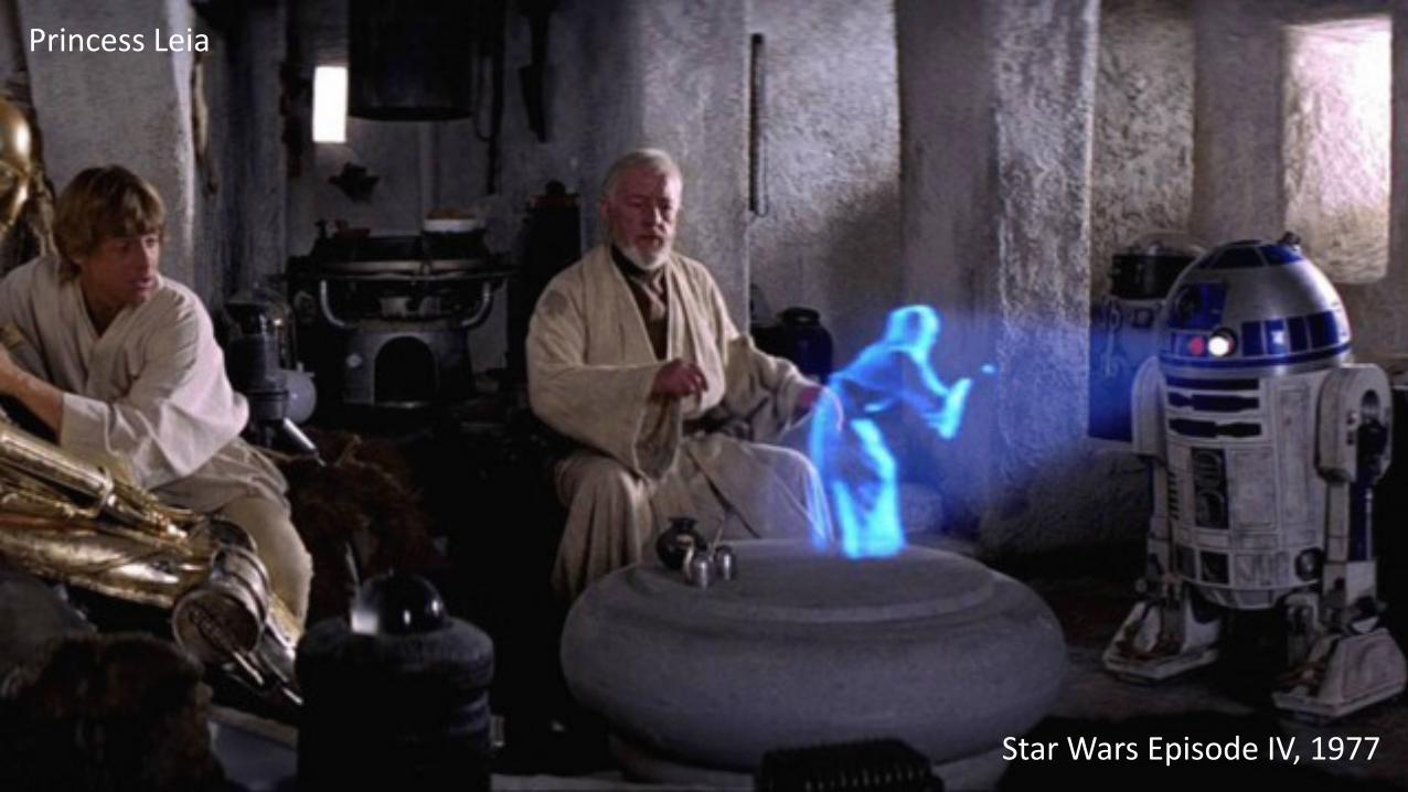
Star Wars Episode IV, 1977

Princess Leia

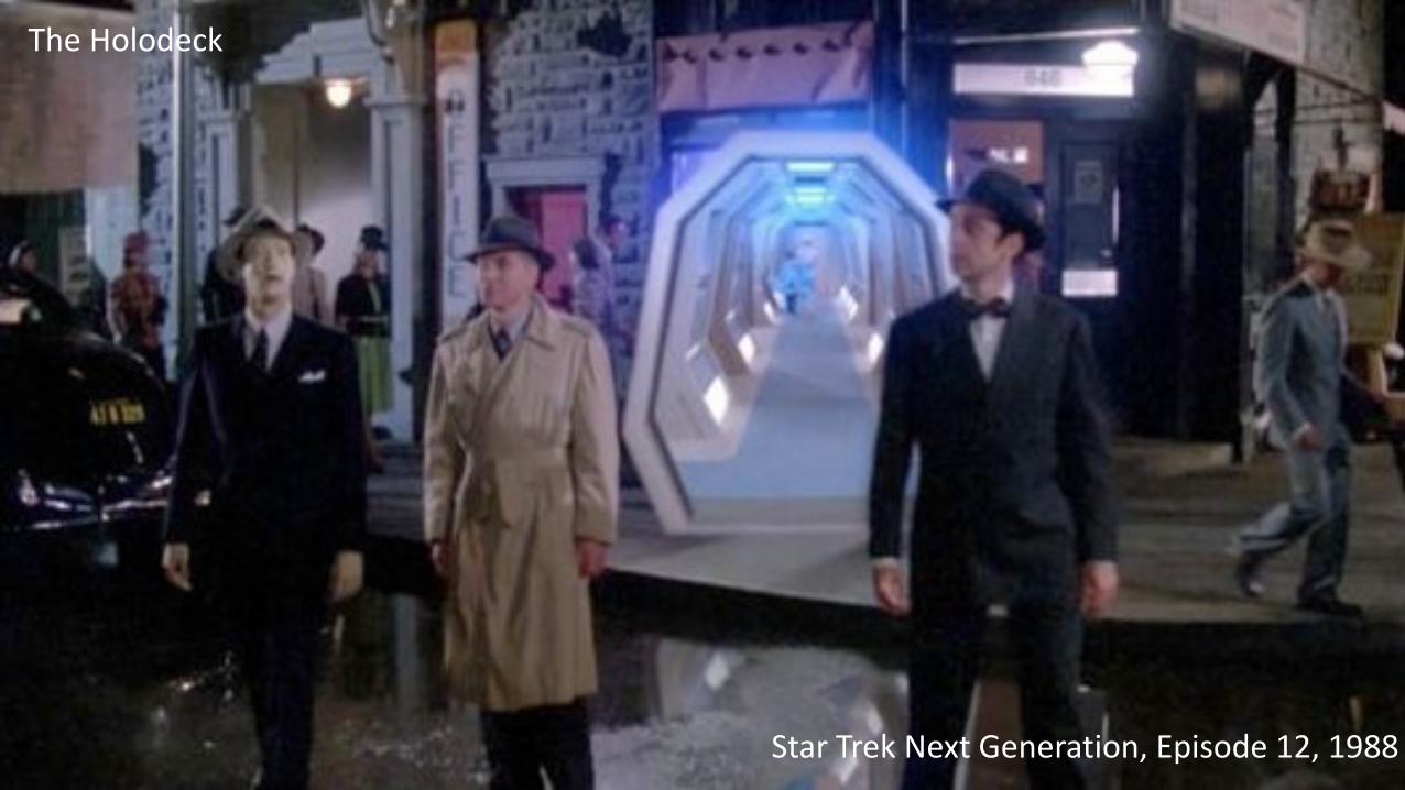
Star Trek Next Generation, Episode 12, 1988

The Holodeck

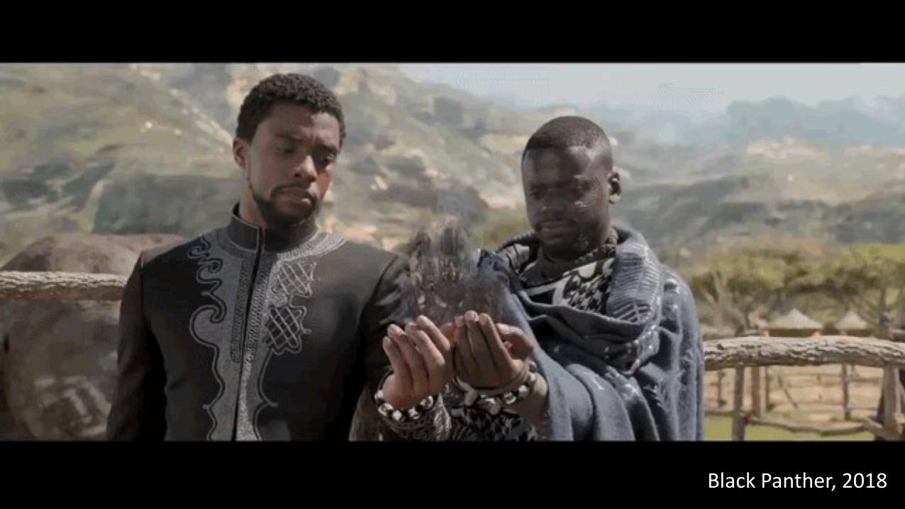
Black Panther, 2018

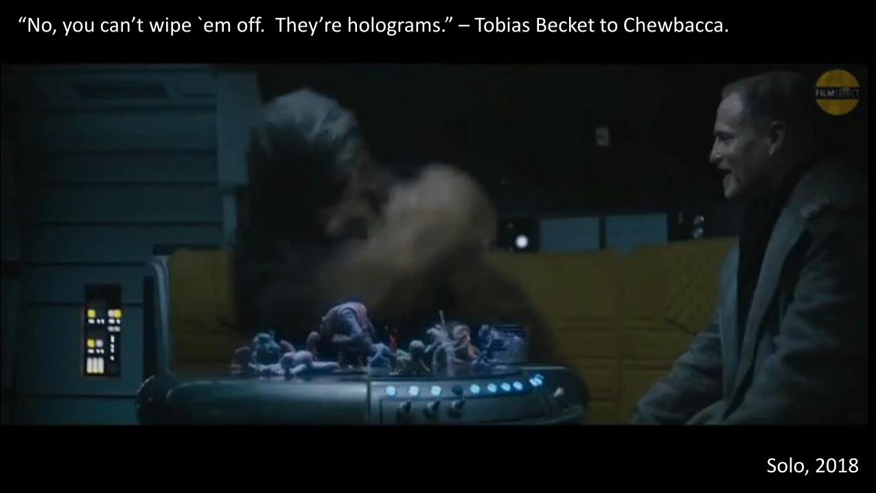
Solo, 2018

“No, you can’t wipe `em off. They’re holograms.” – Tobias Becket to Chewbacca.

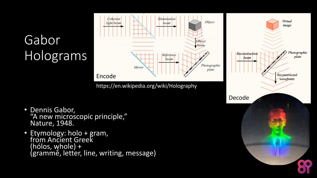
GaborHolograms

• Dennis Gabor,“A new microscopic principle,”Nature, 1948.

• Etymology: holo + gram,from Ancient Greek(hólos, whole) +(grammḗ, letter, line, writing, message)

Decode

Encode

https://en.wikipedia.org/wiki/Holography

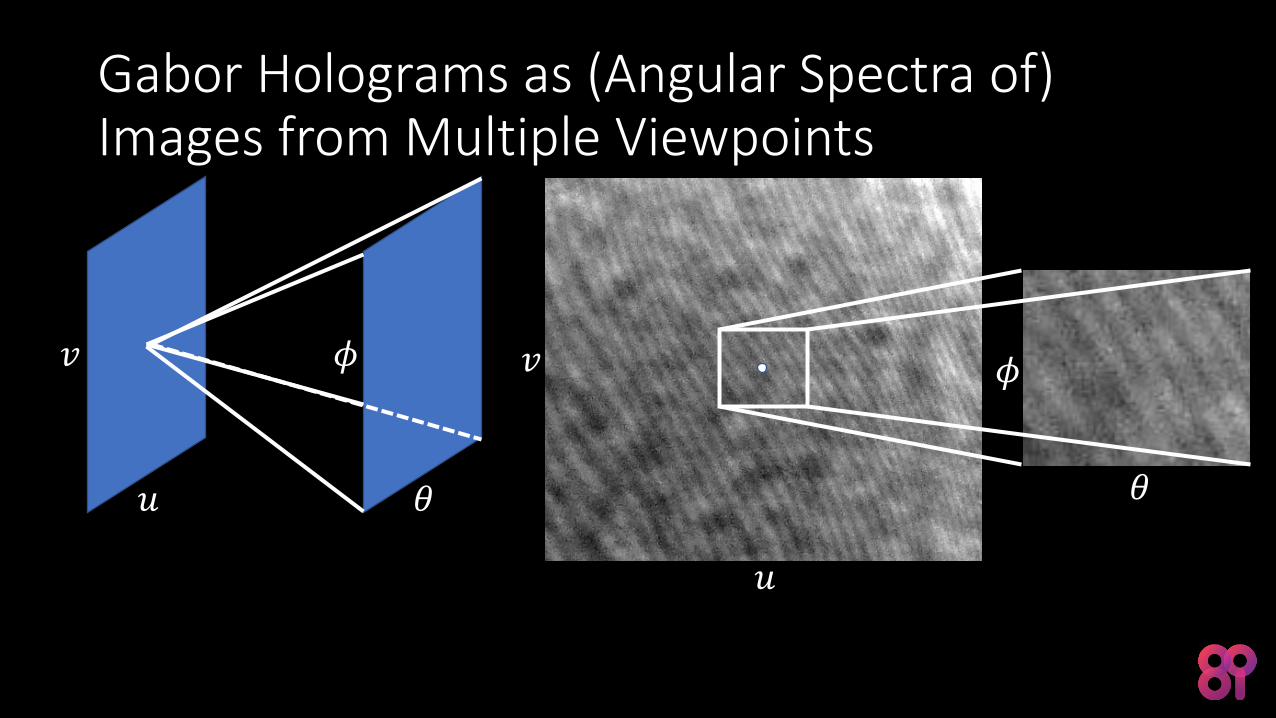
Gabor Holograms as (Angular Spectra of) Images from Multiple Viewpoints

𝑣

𝑢 𝜃

𝜙 𝑣

𝑢

𝜃

𝜙

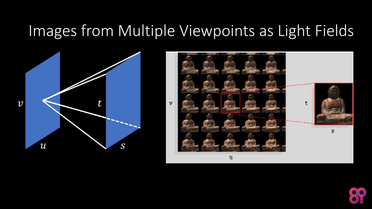
Images from Multiple Viewpoints as Light Fields

𝑣

𝑢 𝑠

𝑡

Light Fields as Point Clouds

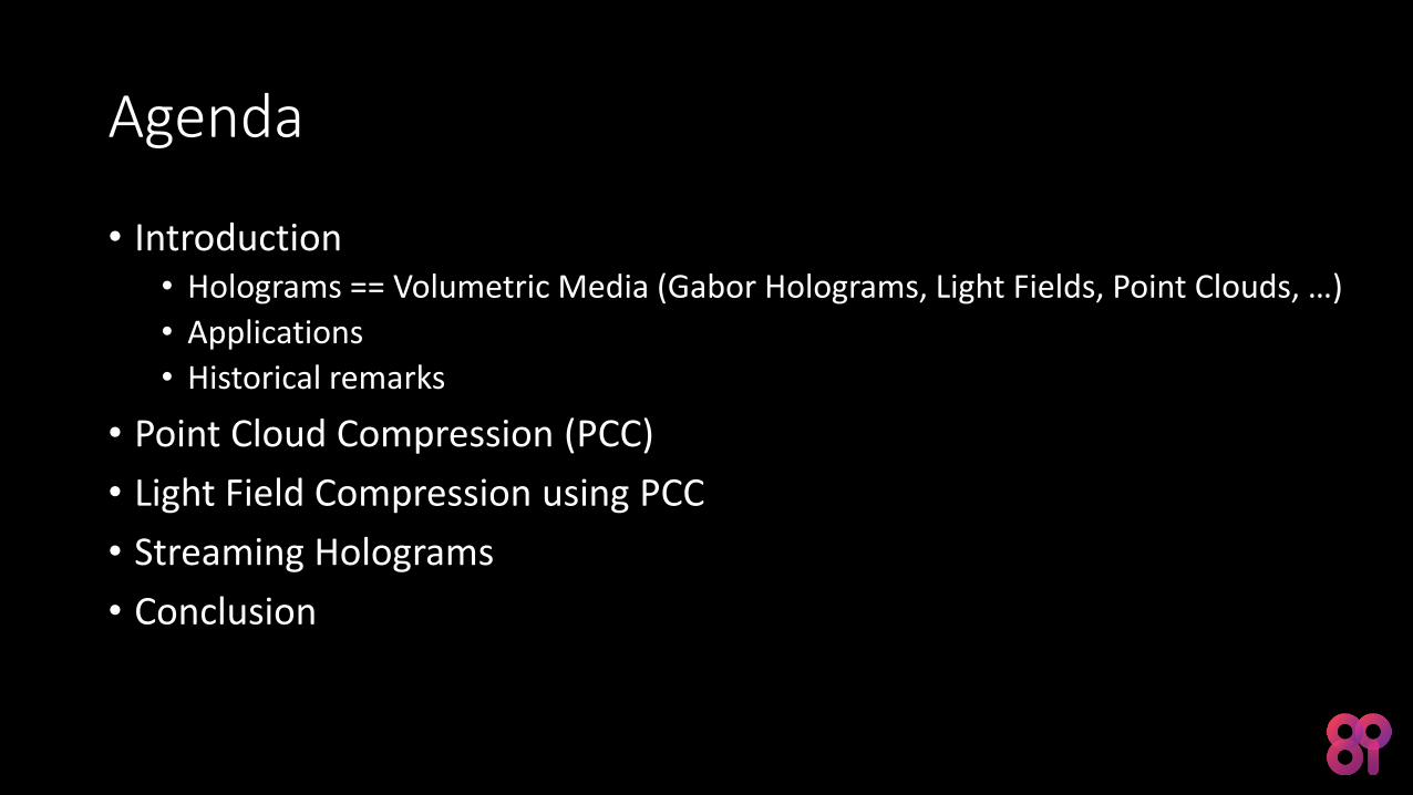
Agenda

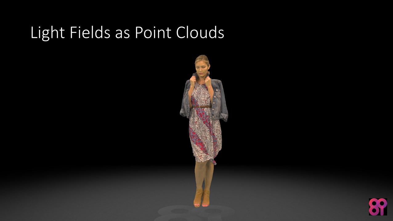
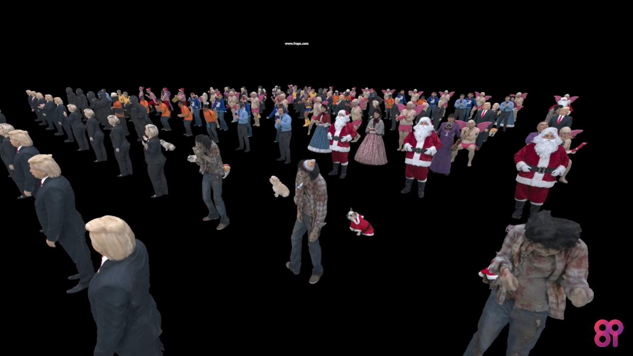
• Introduction• Holograms == Volumetric Media (Gabor Holograms, Light Fields, Point Clouds, …)

• Applications

• Historical remarks

• Point Cloud Compression (PCC)

• Light Field Compression using PCC

• Streaming Holograms

• Conclusion

Applications

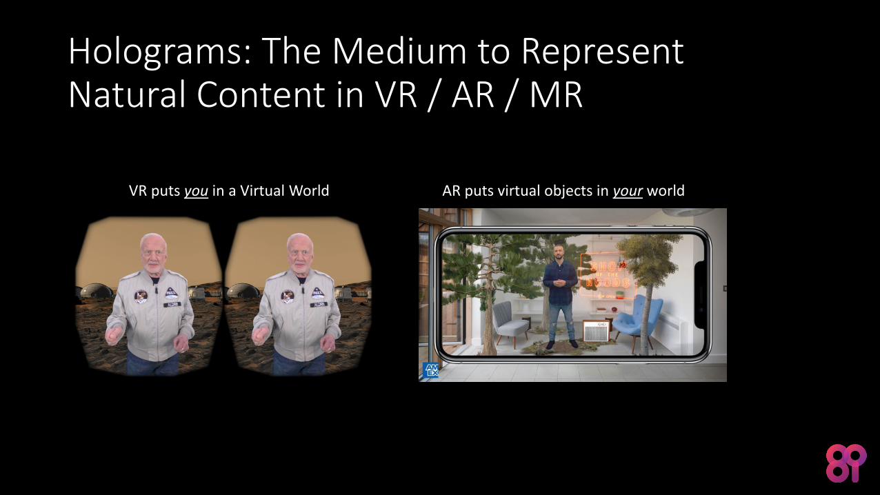
Holograms: The Medium to Represent Natural Content in VR / AR / MR

VR puts you in a Virtual World AR puts virtual objects in your world

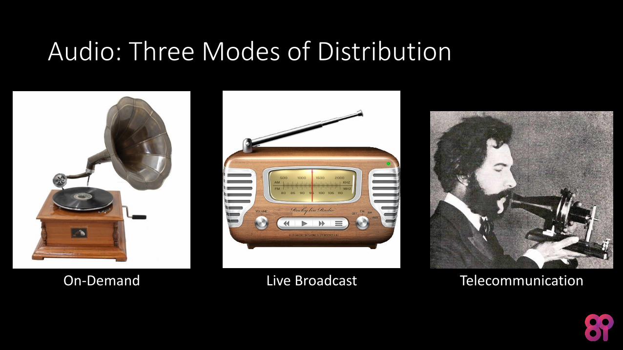
Audio: Three Modes of Distribution

On-Demand Live Broadcast Telecommunication

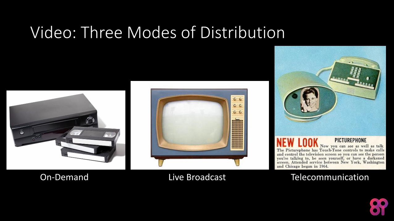
Video: Three Modes of Distribution

On-Demand Live Broadcast Telecommunication

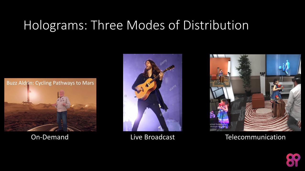
Holograms: Three Modes of Distribution

On-Demand Live Broadcast Telecommunication

Buzz Aldrin: Cycling Pathways to Mars

Historical Remarks

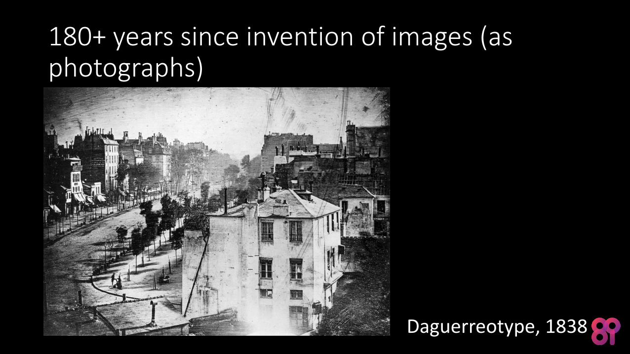
180+ years since invention of images (as photographs)

Daguerreotype, 1838

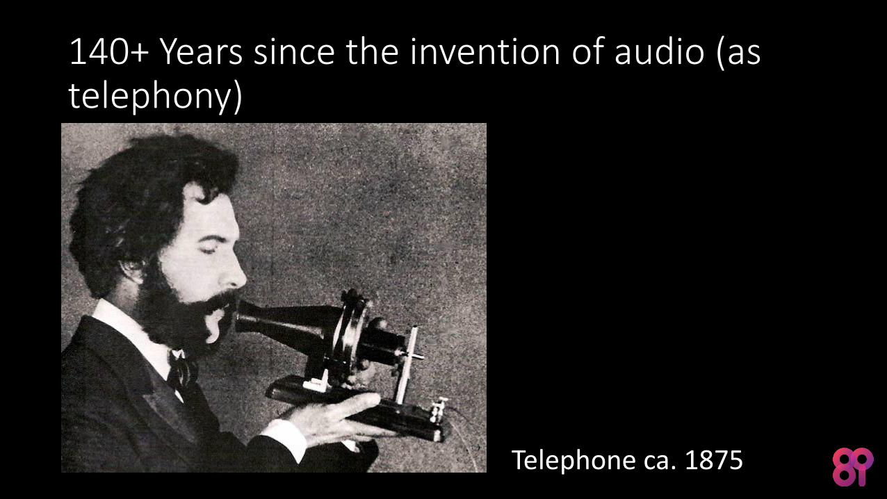
140+ Years since the invention of audio (as telephony)

Telephone ca. 1875

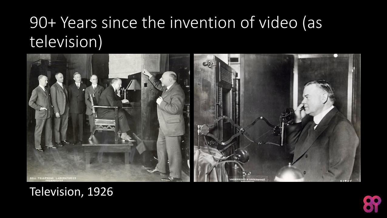
90+ Years since the invention of video (as television)

Television, 1926

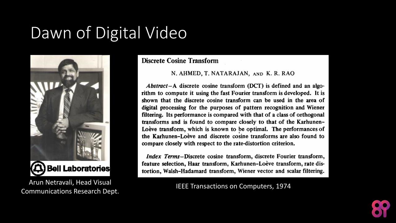
Dawn of Digital Video

Arun Netravali, Head Visual Communications Research Dept.

IEEE Transactions on Computers, 1974

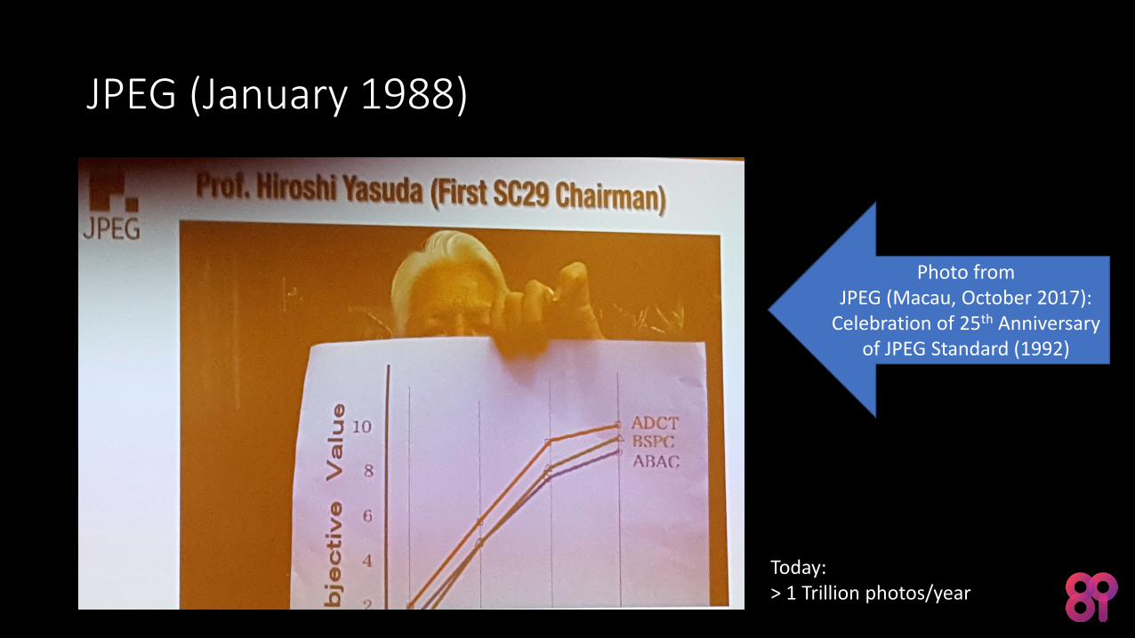
JPEG (January 1988)

Today:> 1 Trillion photos/year

Photo fromJPEG (Macau, October 2017):

Celebration of 25th Anniversary of JPEG Standard (1992)

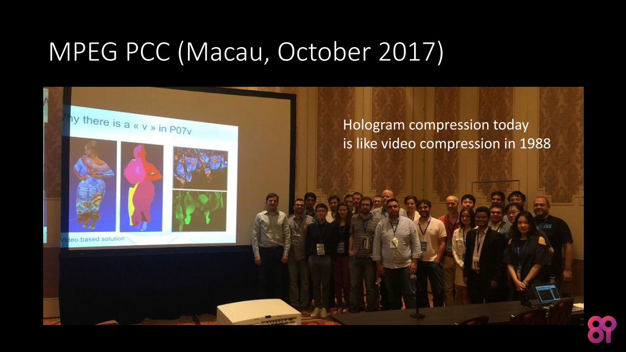
MPEG PCC (Macau, October 2017)

Hologram compression todayis like video compression in 1988

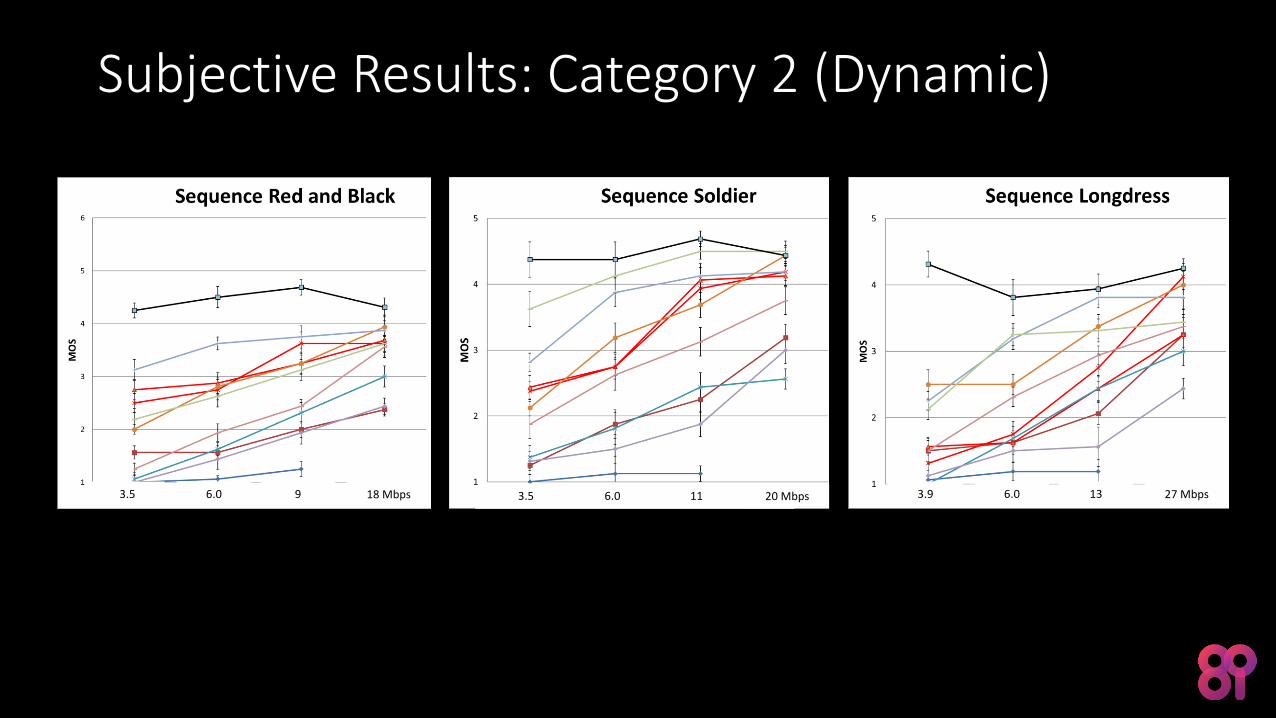
Subjective Results: Category 2 (Dynamic)

3.9 6.0 13 27 Mbps3.5 6.0 11 20 Mbps3.5 6.0 9 18 Mbps

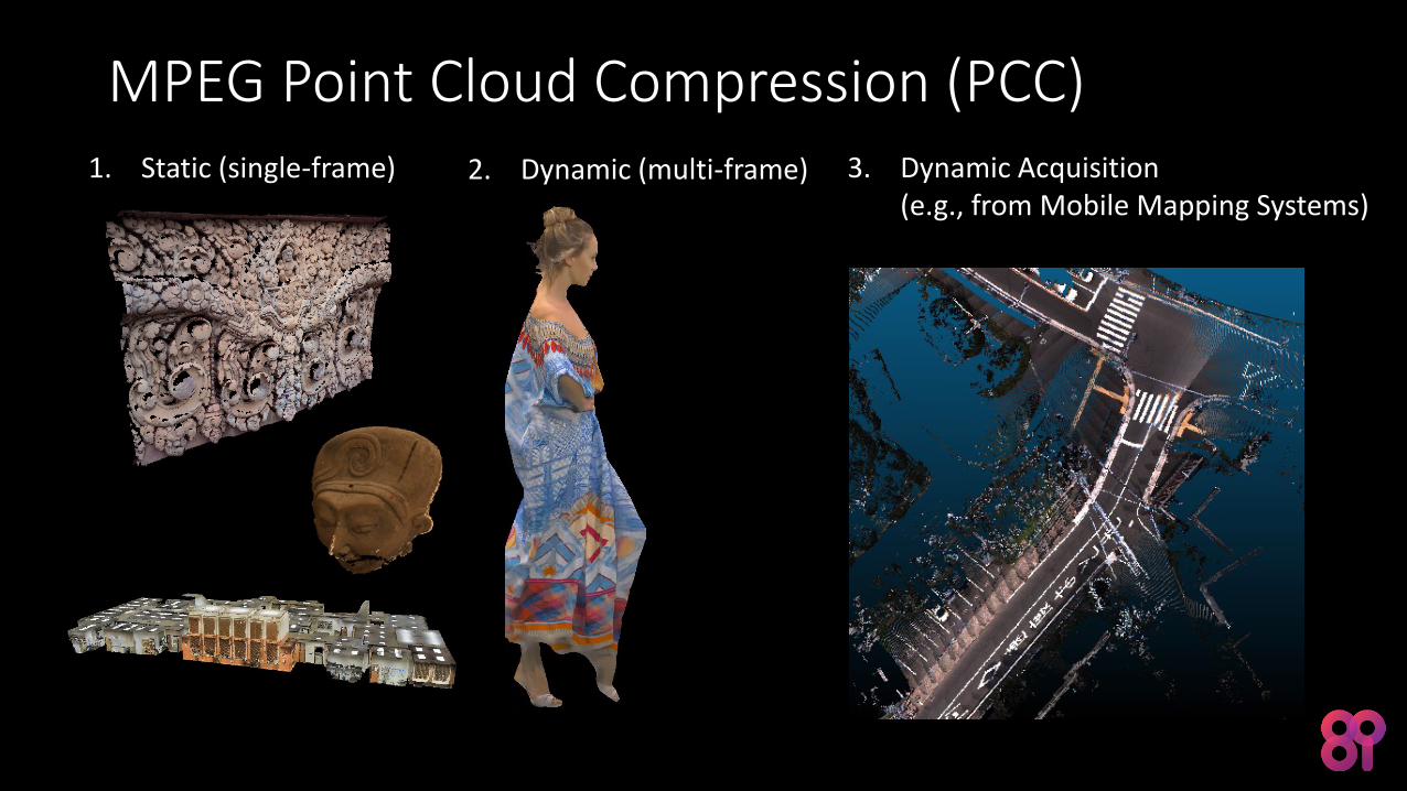
1. Static (single-frame) 3. Dynamic Acquisition(e.g., from Mobile Mapping Systems)

MPEG Point Cloud Compression (PCC)2. Dynamic (multi-frame)

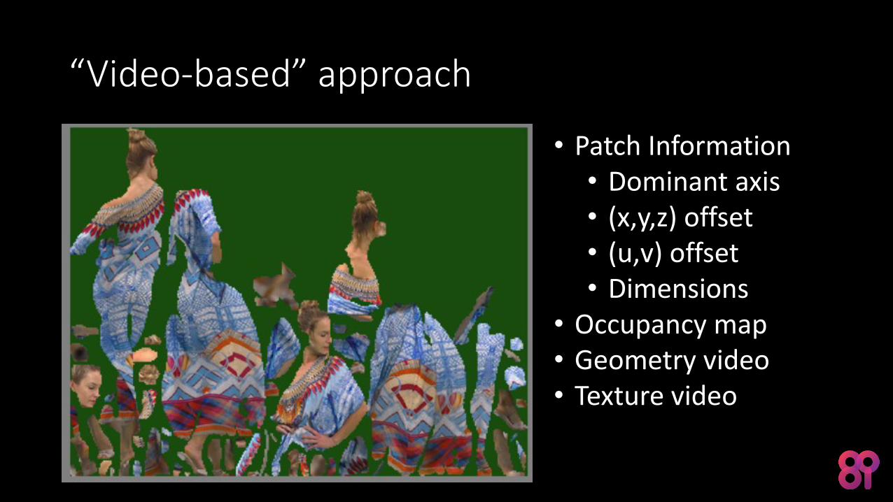
“Video-based” approach

• Patch Information• Dominant axis• (x,y,z) offset• (u,v) offset• Dimensions

• Occupancy map• Geometry video• Texture video

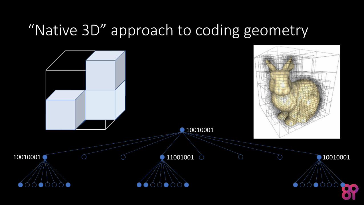
“Native 3D” approach to coding geometry

10010001

10010001 11001001 10010001

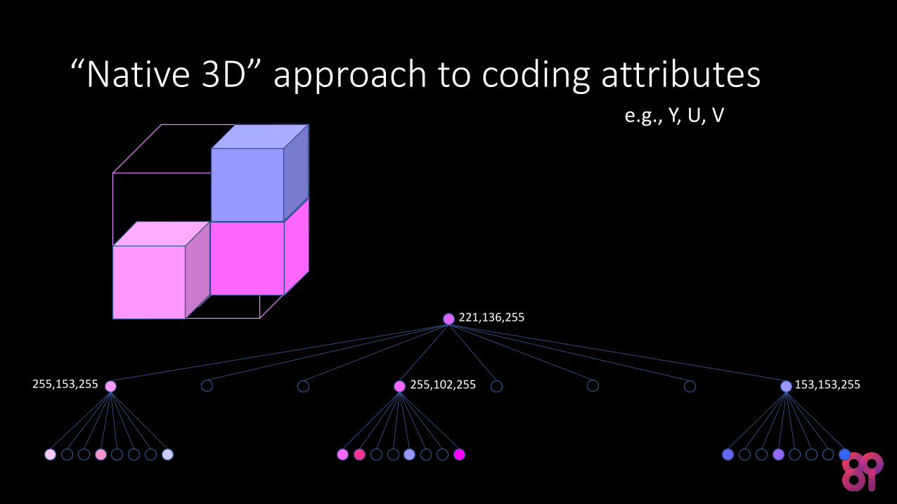
“Native 3D” approach to coding attributes

221,136,255

255,153,255 255,102,255 153,153,255

e.g., Y, U, V

Point Cloud Attribute Compression using a Region Adaptive Hierarchical Transform (RAHT)Ricardo L. de Queiroz and Philip A. Chou, “Compression of 3D Point Clouds Using a Region-Adaptive Hierarchical Transform,” IEEE Trans. Image Processing, Aug 2016.

Maja Krivokuca, Maxim Koroteev, Philip A. Chou, Robert Higgs, and Charles Loop, “A Volumetric Approach to Point Cloud Compression,” in preparation.

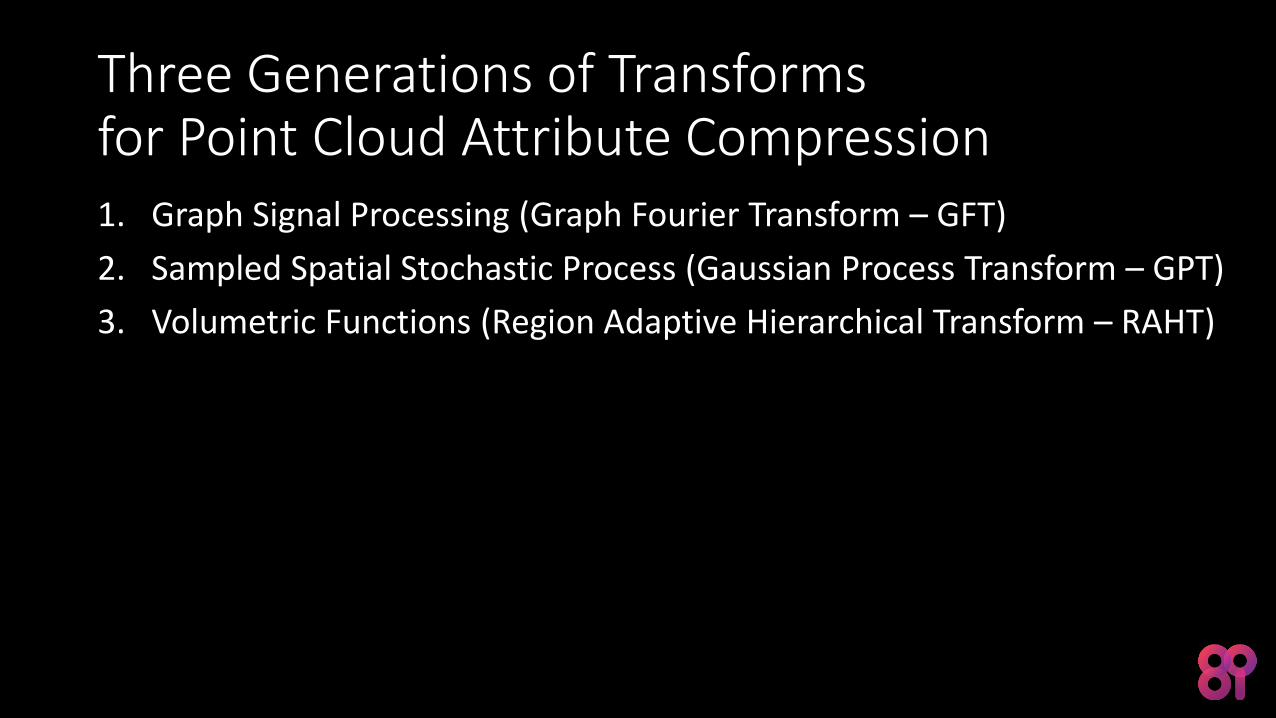
Three Generations of Transformsfor Point Cloud Attribute Compression1. Graph Signal Processing (Graph Fourier Transform – GFT)

2. Sampled Spatial Stochastic Process (Gaussian Process Transform – GPT)

3. Volumetric Functions (Region Adaptive Hierarchical Transform – RAHT)

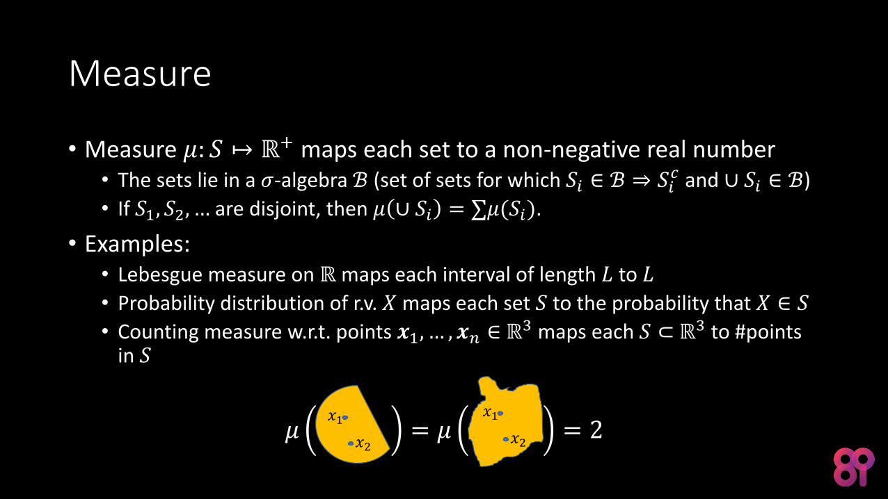
Measure

• Measure 𝜇: 𝑆 ↦ ℝ+ maps each set to a non-negative real number• The sets lie in a 𝜎-algebra ℬ (set of sets for which 𝑆𝑖 ∈ ℬ ⇒ 𝑆𝑖

𝑐 and ∪ 𝑆𝑖 ∈ ℬ)

• If 𝑆1, 𝑆2, … are disjoint, then 𝜇 ∪ 𝑆𝑖 = ∑𝜇(𝑆𝑖).

• Examples:• Lebesgue measure on ℝ maps each interval of length 𝐿 to 𝐿

• Probability distribution of r.v. 𝑋 maps each set 𝑆 to the probability that 𝑋 ∈ 𝑆

• Counting measure w.r.t. points 𝒙1, … , 𝒙𝑛 ∈ ℝ3 maps each 𝑆 ⊂ ℝ3 to #points

in 𝑆

𝜇 = 𝜇 = 2𝑥2

𝑥1𝑥2

𝑥1

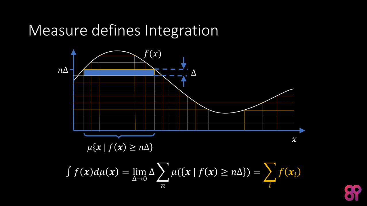
Measure defines Integration

∫ 𝑓 𝒙 𝑑𝜇 𝒙 = limΔ→0

Δ

𝑛

𝜇( 𝒙 | 𝑓 𝒙 ≥ 𝑛Δ ) =

𝑖

𝑓 𝒙𝑖

𝑛Δ

𝜇 𝒙 | 𝑓 𝒙 ≥ 𝑛Δ

𝑓(𝑥)

𝑥

Δ

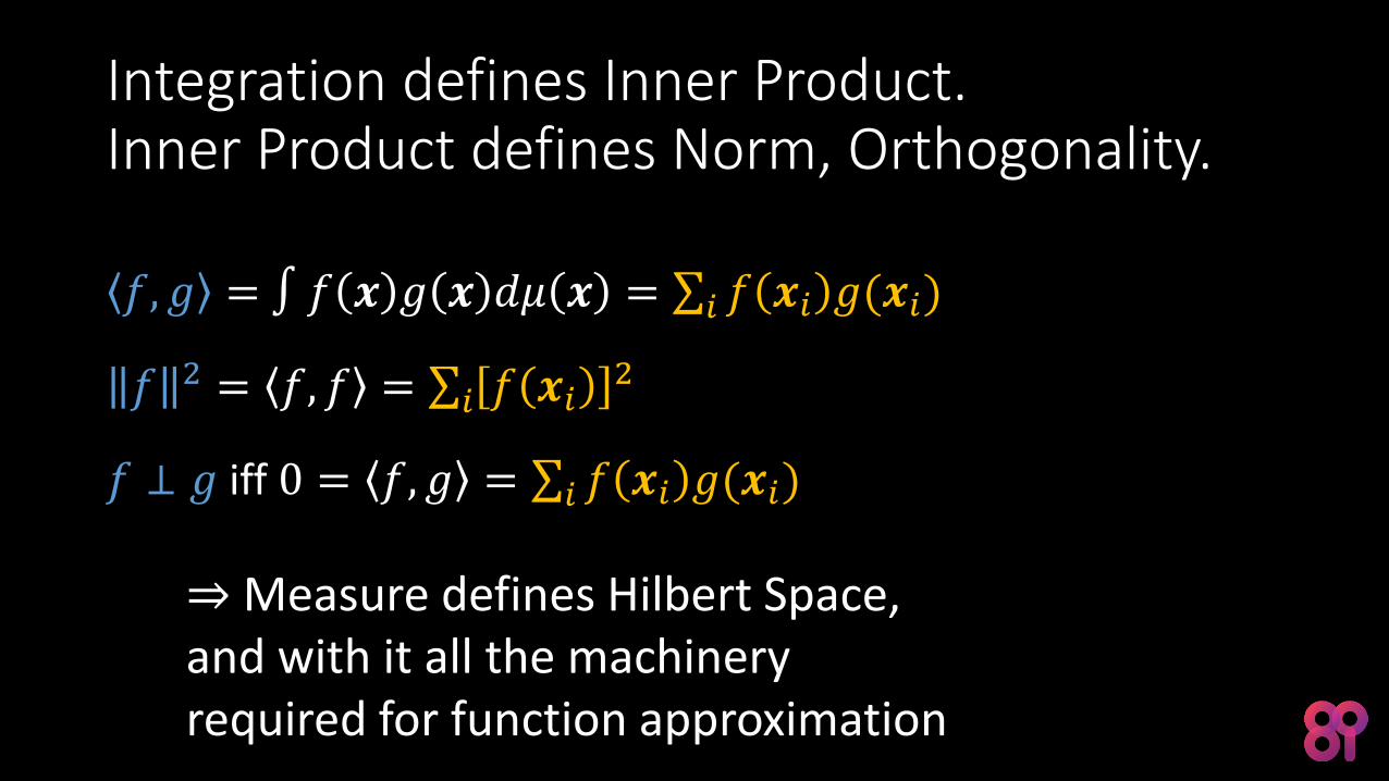
Integration defines Inner Product.Inner Product defines Norm, Orthogonality.

𝑓, 𝑔 = ∫ 𝑓 𝒙 𝑔 𝒙 𝑑𝜇 𝒙 = ∑𝑖 𝑓 𝒙𝑖 𝑔(𝒙𝑖)

𝑓 2 = 𝑓, 𝑓 = ∑𝑖 𝑓 𝒙𝑖2

𝑓 ⊥ 𝑔 iff 0 = 𝑓, 𝑔 = ∑𝑖 𝑓 𝒙𝑖 𝑔(𝒙𝑖)

⇒ Measure defines Hilbert Space, and with it all the machinery required for function approximation

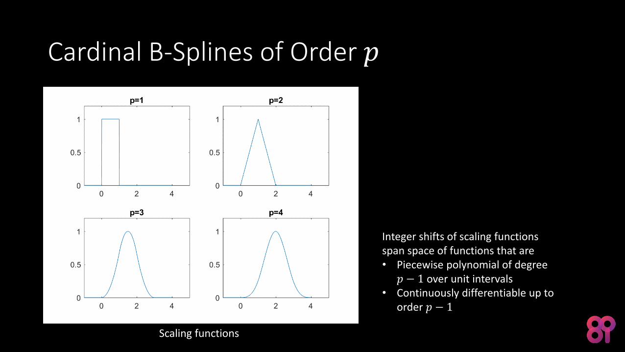
Cardinal B-Splines of Order 𝑝

Scaling functions

Integer shifts of scaling functions span space of functions that are• Piecewise polynomial of degree

𝑝 − 1 over unit intervals• Continuously differentiable up to

order 𝑝 − 1

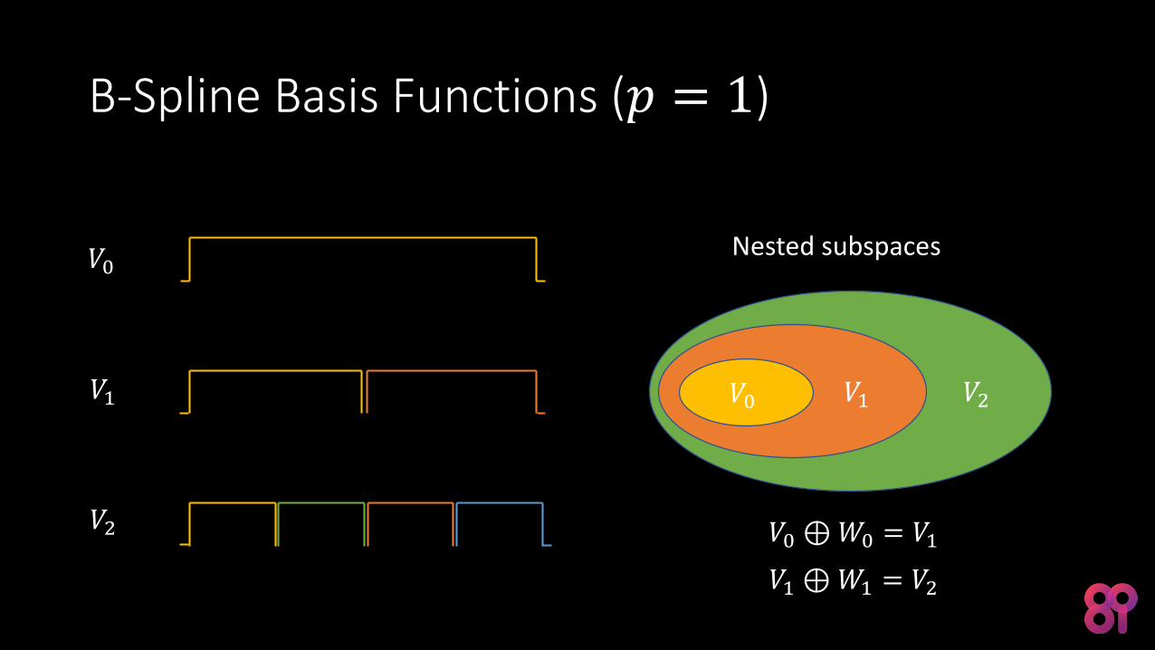
B-Spline Basis Functions (𝑝 = 1)

𝑉0

𝑉1

𝑉2

𝑉2𝑉1𝑉0

𝑉0 ⊕𝑊0 = 𝑉1

𝑉1 ⊕𝑊1 = 𝑉2

Nested subspaces

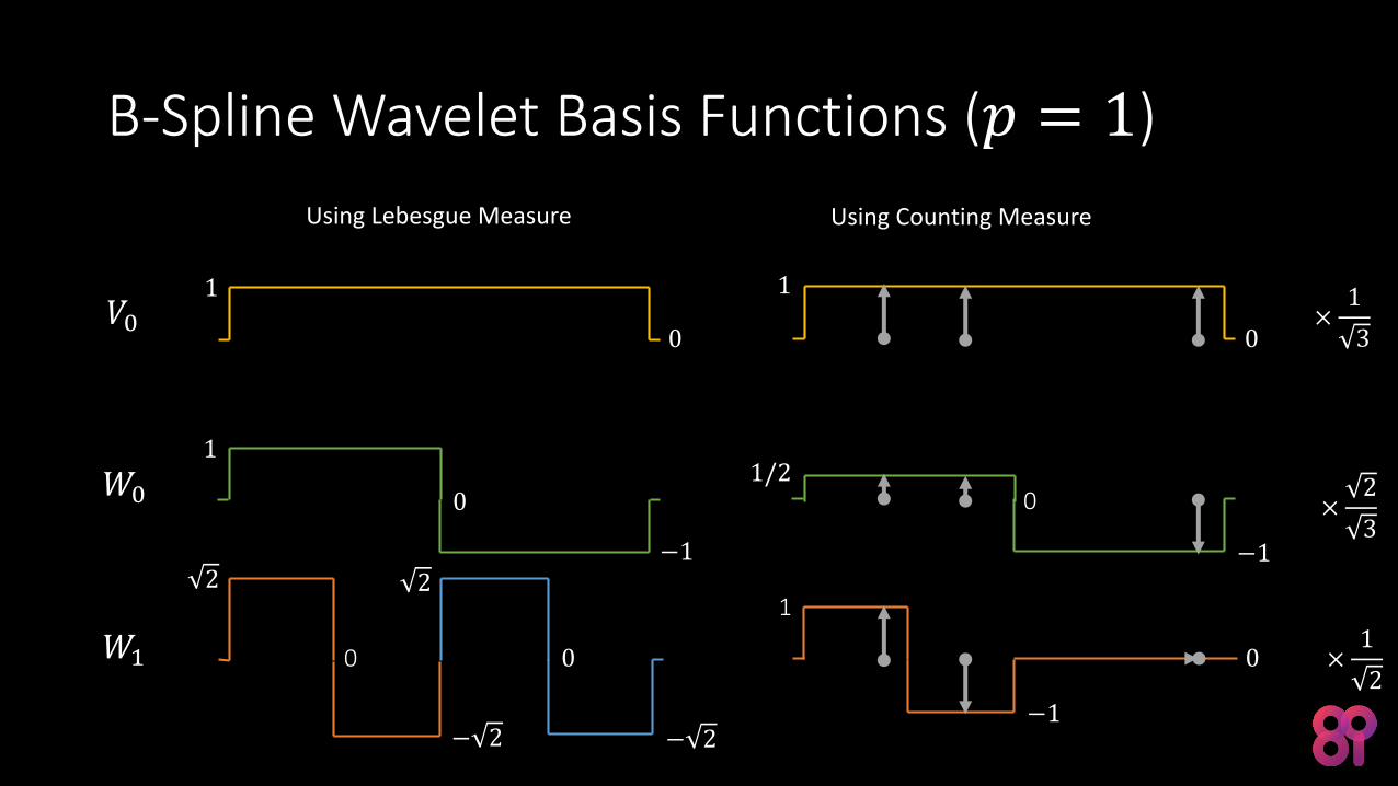
B-Spline Wavelet Basis Functions (𝑝 = 1)

Using Lebesgue Measure Using Counting Measure

𝑉0

𝑊0

𝑊1

1

1

2

1

1/2

1

−1

− 2

0 0

−1

0

−1

0 0

0

− 2

0

2

×1

3

×2

3

×1

2

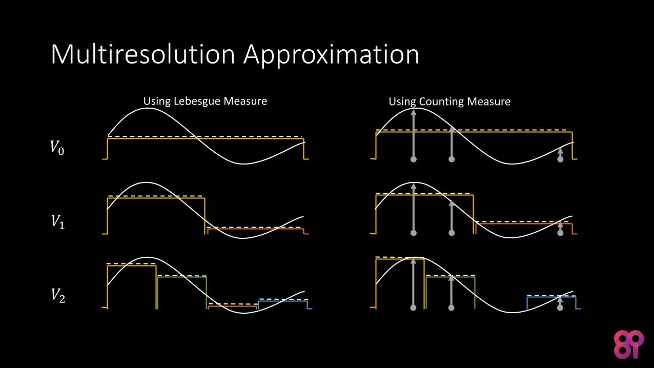
Multiresolution Approximation

𝑉0

𝑉1

𝑉2

Using Lebesgue Measure Using Counting Measure

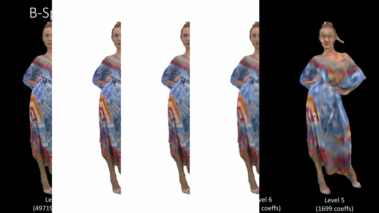
B-Spline Approximation (𝑝 = 1)

Level 7(15604 coeffs)

Level 6(3821 coeffs)

Level 5(917 coeffs)

Level 8(62073 coeffs)

Level 9(237965 coeffs)

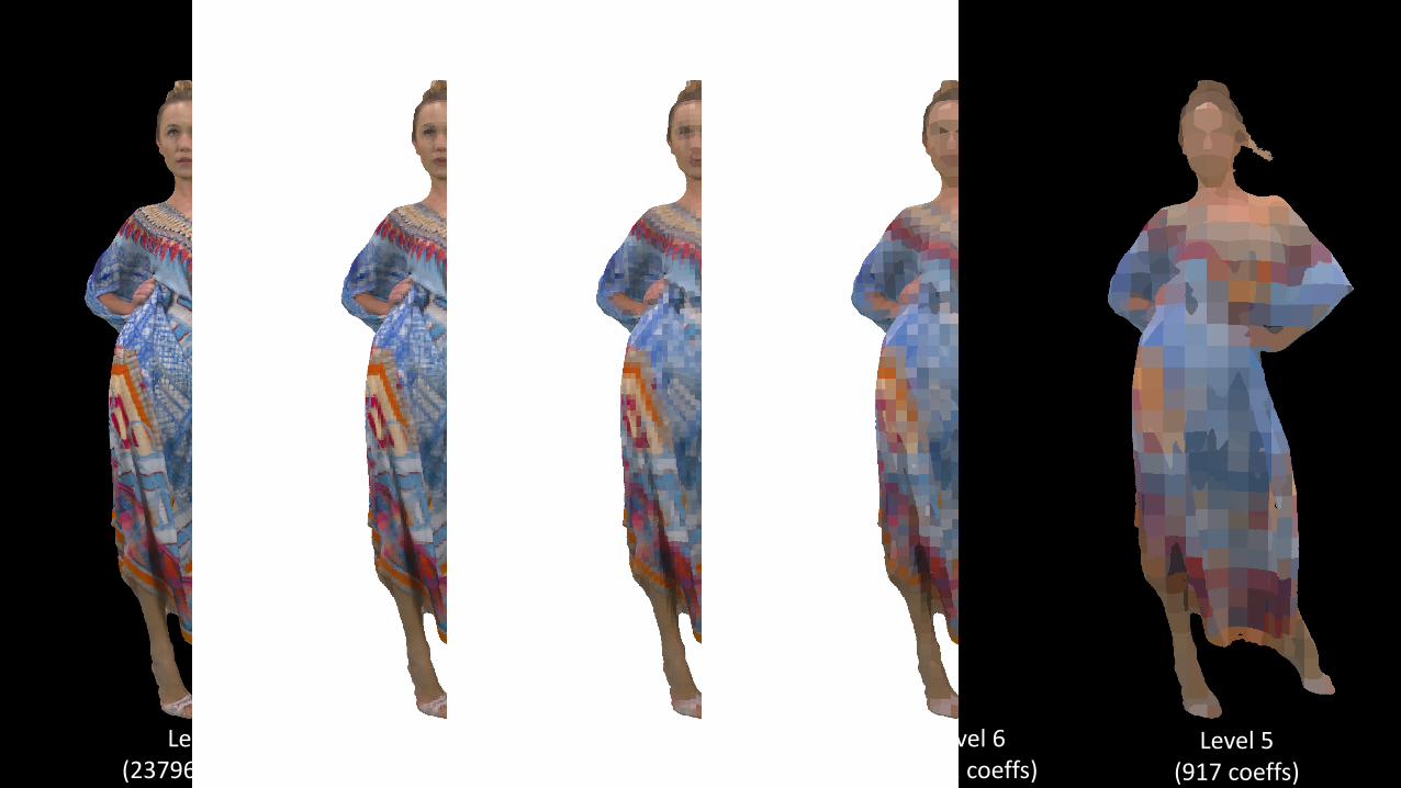
B-Spline Approximation (𝑝 = 2)

Level 7(30455 coeffs)

Level 6(7213 coeffs)

Level 5(1699 coeffs)

Level 8(125244 coeffs)

Level 9(497199 coeffs)

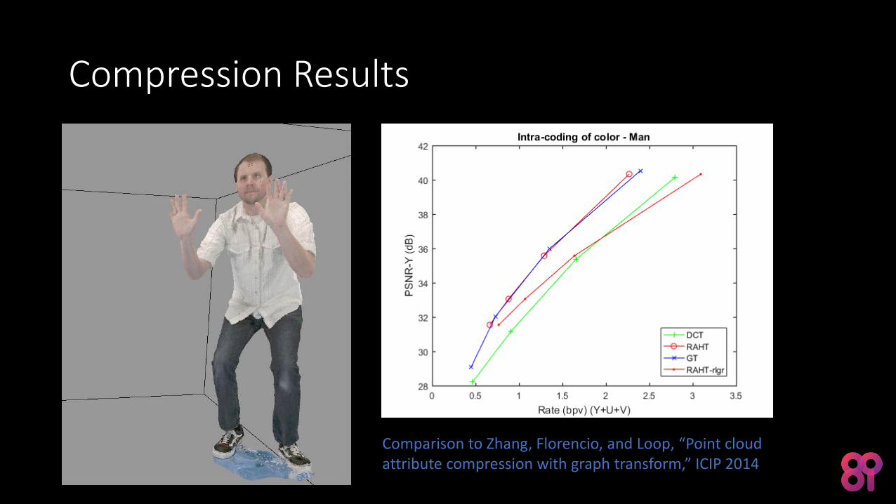
Compression Results

Comparison to Zhang, Florencio, and Loop, “Point cloud attribute compression with graph transform,” ICIP 2014

Surface Light Field Compression using a Point Cloud CodecXiang Zhang, Philip A. Chou, Ming-Ting Sun, Maolong Yang, et al., “Surface Light Field Compression using a Point Cloud Codec,” submitted to IEEE JETCAS special issue on immersive video, and to appear at ICIP 2018.

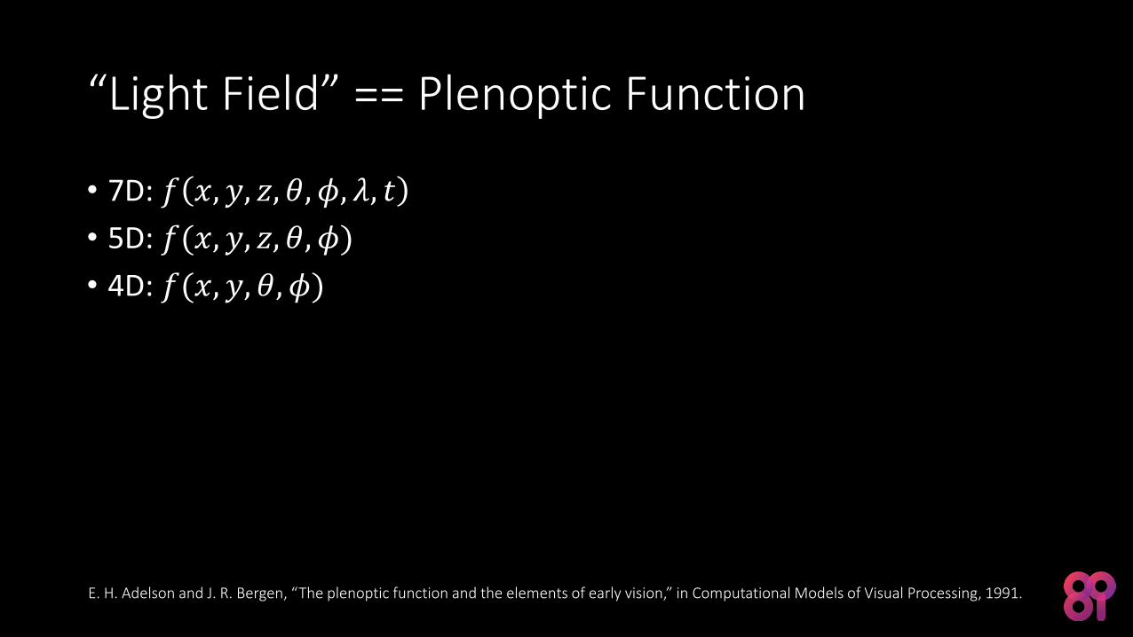
“Light Field” == Plenoptic Function

• 7D: 𝑓 𝑥, 𝑦, 𝑧, 𝜃, 𝜙, 𝜆, 𝑡

• 5D: 𝑓(𝑥, 𝑦, 𝑧, 𝜃, 𝜙)

• 4D: 𝑓(𝑥, 𝑦, 𝜃, 𝜙)

E. H. Adelson and J. R. Bergen, “The plenoptic function and the elements of early vision,” in Computational Models of Visual Processing, 1991.

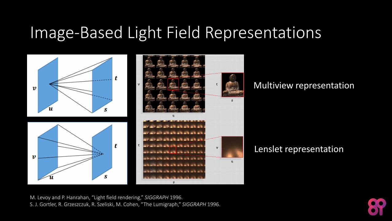
Image-Based Light Field Representations

M. Levoy and P. Hanrahan, “Light field rendering,” SIGGRAPH 1996.S. J. Gortler, R. Grzeszczuk, R. Szeliski, M. Cohen, “The Lumigraph,” SIGGRAPH 1996.

Multiview representation

Lenslet representation

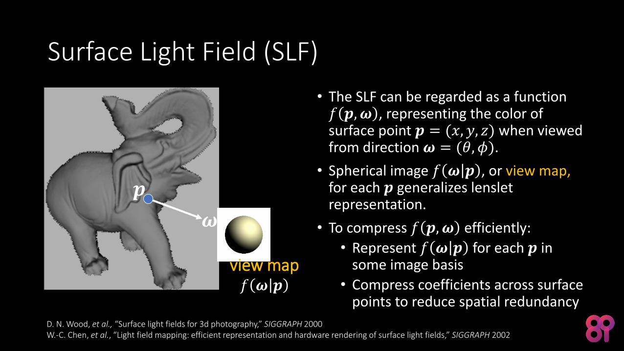
Surface Light Field (SLF)

• The SLF can be regarded as a function 𝑓 𝒑,𝝎 , representing the color of surface point 𝒑 = (𝑥, 𝑦, 𝑧) when viewed from direction 𝝎 = (𝜃, 𝜙).

• Spherical image 𝑓 𝝎 𝒑 , or view map, for each 𝒑 generalizes lenslet representation.

• To compress 𝑓 𝒑,𝝎 efficiently:

• Represent 𝑓 𝝎 𝒑 for each 𝒑 in some image basis

• Compress coefficients across surface points to reduce spatial redundancy

D. N. Wood, et al., “Surface light fields for 3d photography,” SIGGRAPH 2000W.-C. Chen, et al., “Light field mapping: efficient representation and hardware rendering of surface light fields,” SIGGRAPH 2002

𝒑

𝝎

view map𝑓 𝝎 𝒑

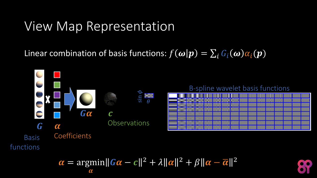
View Map Representation

Linear combination of basis functions: 𝑓 𝝎 𝒑 = ∑𝑖 𝐺𝑖 𝝎 𝛼𝑖(𝒑)

Basisfunctions

𝒄𝑮𝜶

𝑮 𝜶Coefficients

Observations

B-spline wavelet basis functions

𝜶 = argmin𝜶

𝑮𝜶 − 𝒄 2 + 𝜆 𝜶 2 + 𝛽 𝜶 − ഥ𝜶 2

𝜃sin𝜙

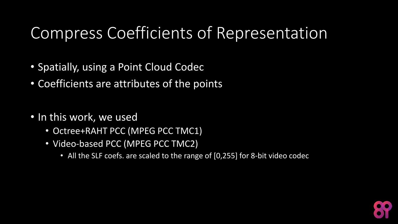
Compress Coefficients of Representation

• Spatially, using a Point Cloud Codec

• Coefficients are attributes of the points

• In this work, we used• Octree+RAHT PCC (MPEG PCC TMC1)

• Video-based PCC (MPEG PCC TMC2)• All the SLF coefs. are scaled to the range of [0,255] for 8-bit video codec

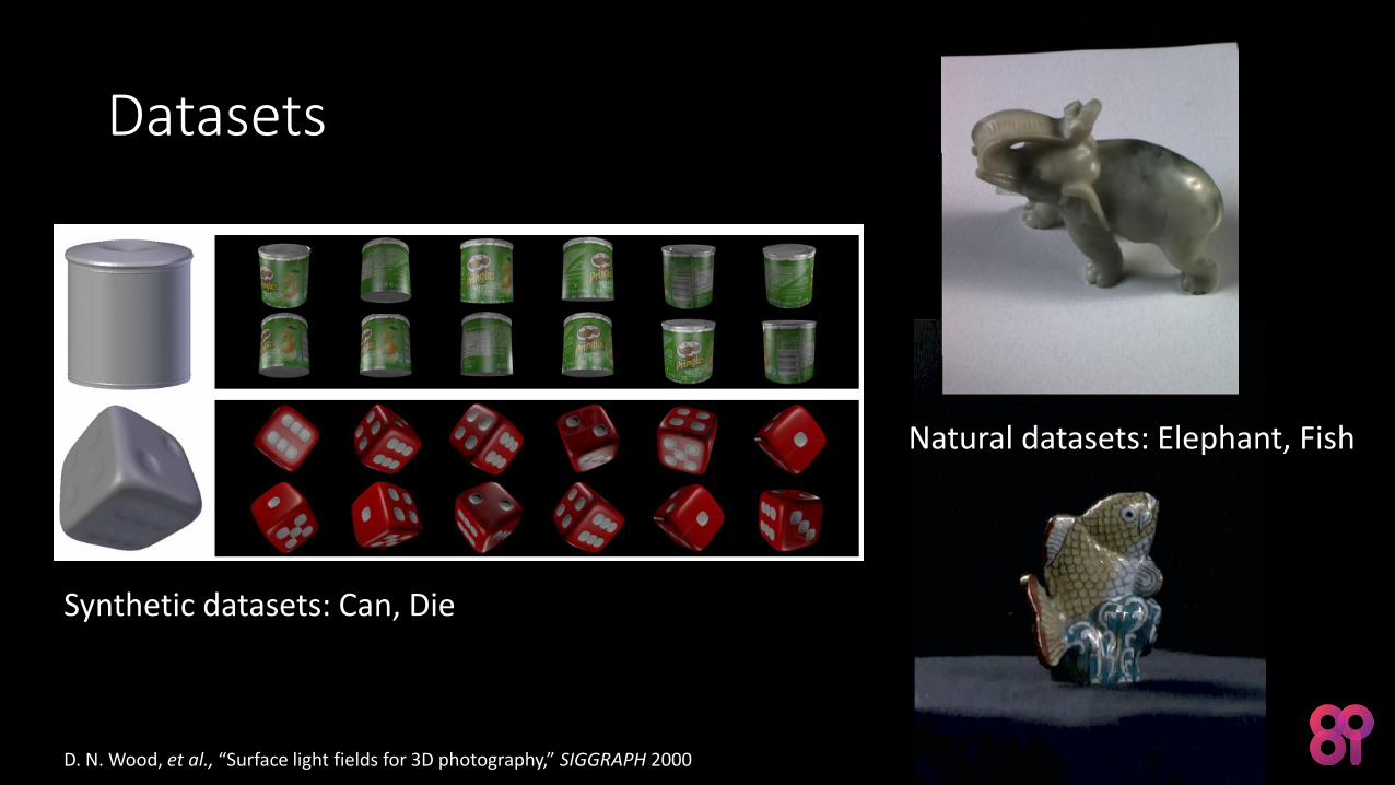
Datasets

Synthetic datasets: Can, Die

Natural datasets: Elephant, Fish

D. N. Wood, et al., “Surface light fields for 3D photography,” SIGGRAPH 2000

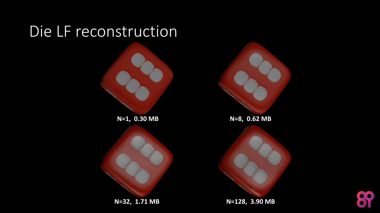
Die LF reconstruction

N=1, 0.30 MB N=8, 0.62 MB

N=32, 1.71 MB N=128, 3.90 MB

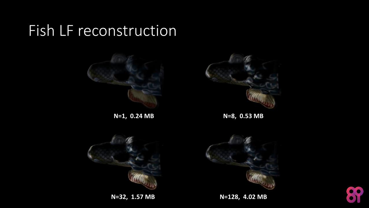
Fish LF reconstruction

N=1, 0.24 MB N=8, 0.53 MB

N=32, 1.57 MB N=128, 4.02 MB

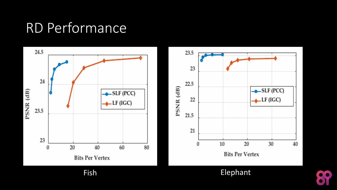
RD Performance

Fish Elephant

Streaming of Volumetric MediaJounsup Park, Philip A. Chou, and Jenq-Neng Hwang, “Rate-Utility Optimized Streaming of Volumetric Media for Augmented Reality,” arXiv:1804.09864.Also submitted to IEEE JETCAS special issue on immersive video,and to appear at Globecom 2018.

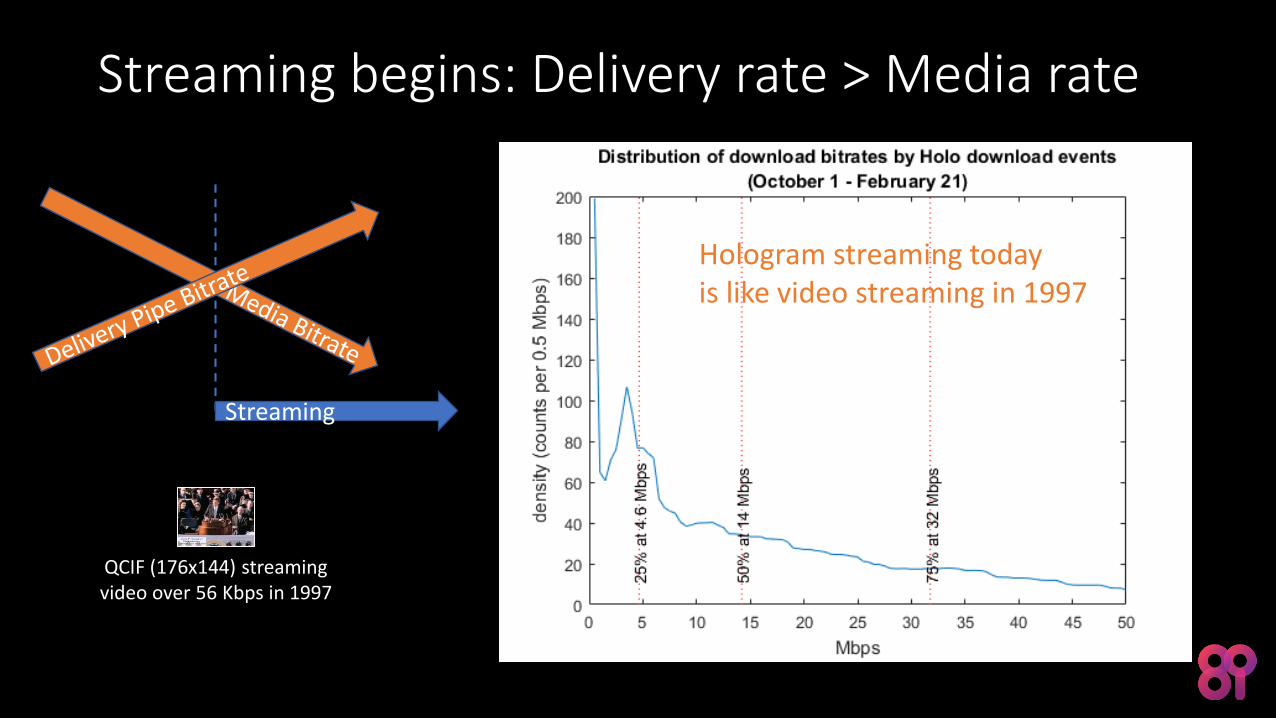
Streaming begins: Delivery rate > Media rate

Streaming

QCIF (176x144) streaming video over 56 Kbps in 1997

Hologram streaming todayis like video streaming in 1997

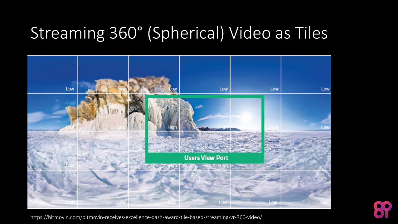
Streaming 360° (Spherical) Video as Tiles

https://bitmovin.com/bitmovin-receives-excellence-dash-award-tile-based-streaming-vr-360-video/

https://d.docs.live.net/5b20c30bf1023c52/Pubs/Presentations/180614 MMSys - Keynote/zaxisbacktowardfront.mp4

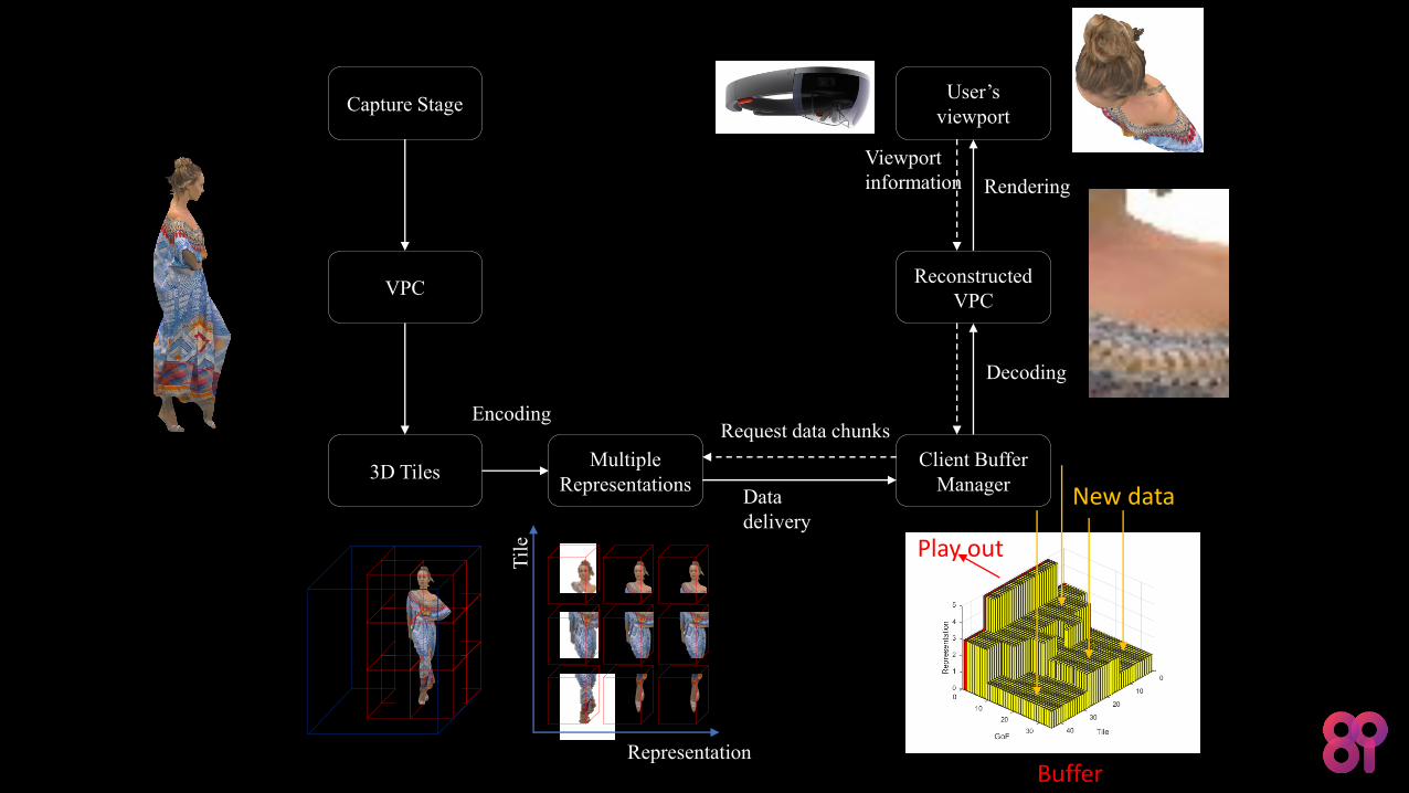
Capture Stage

VPC

3D TilesMultiple

Representations

Client Buffer

Manager

Reconstructed

VPC

User’s

viewport

Decoding

Rendering

Request data chunks

Viewport

information

Encoding

Representation

Til

e

Data

delivery

Play out

New data

Buffer

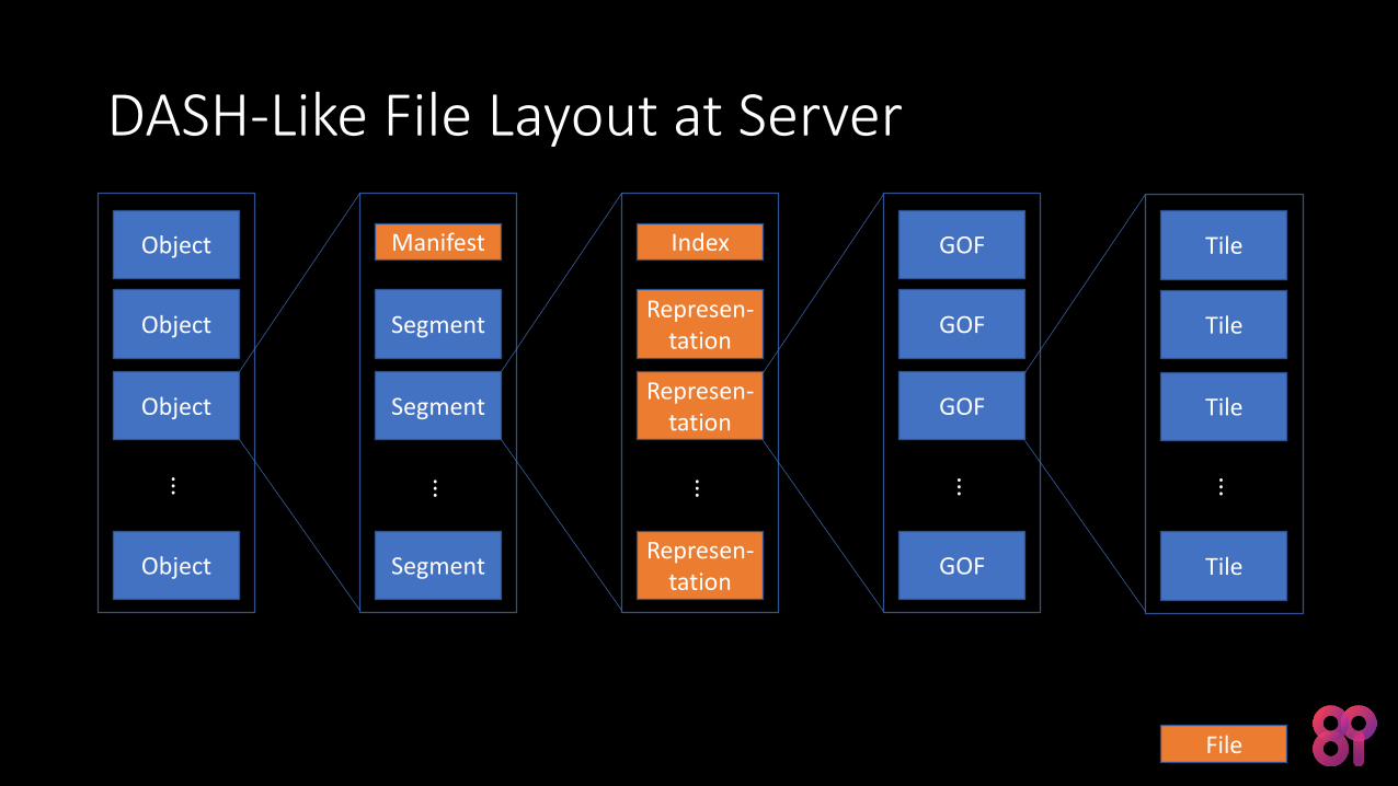
Object

Object

Object

Object

Segment

Manifest

Segment

Segment

Represen-tation

Represen-tation

Represen-tation

GOF

GOF

GOF

GOF

Tile

Tile

Tile

⋮

Tile

Index

⋮⋮⋮⋮

File

DASH-Like File Layout at Server

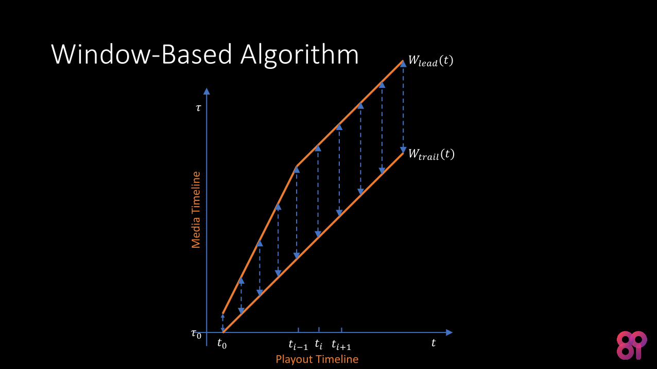
Window-Based Algorithm 𝑊𝑙𝑒𝑎𝑑(𝑡)

𝑊𝑡𝑟𝑎𝑖𝑙(𝑡)

𝑡0 𝑡𝜏0

𝜏

Med

ia T

imel

ine

Playout Timeline

𝑡𝑖 𝑡𝑖+1𝑡𝑖−1

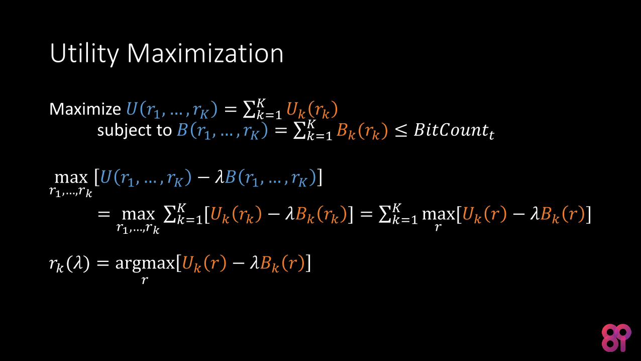
Utility Maximization

Maximize 𝑈 𝑟1, … , 𝑟𝐾 = ∑𝑘=1𝐾 𝑈𝑘 𝑟𝑘

subject to 𝐵 𝑟1, … , 𝑟𝐾 = ∑𝑘=1𝐾 𝐵𝑘(𝑟𝑘) ≤ 𝐵𝑖𝑡𝐶𝑜𝑢𝑛𝑡𝑡

max𝑟1,…,𝑟𝑘

𝑈 𝑟1, … , 𝑟𝐾 − 𝜆𝐵 𝑟1, … , 𝑟𝐾

= max𝑟1,…,𝑟𝑘

∑𝑘=1𝐾 [𝑈𝑘 𝑟𝑘 − 𝜆𝐵𝑘 𝑟𝑘 ] = ∑𝑘=1

𝐾 max𝑟[𝑈𝑘 𝑟 − 𝜆𝐵𝑘 𝑟 ]

𝑟𝑘(𝜆) = argmax𝑟

𝑈𝑘 𝑟 − 𝜆𝐵𝑘 𝑟

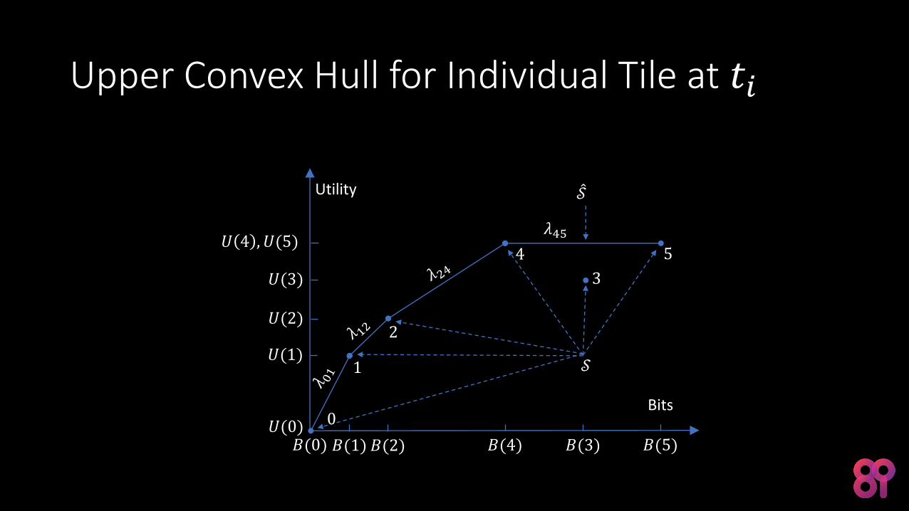
Upper Convex Hull for Individual Tile at 𝑡𝑖

𝐵(4)𝑈(0)

𝑈 4 , 𝑈(5)

𝑈(2)

Utility

𝒮

መ𝒮

5

3

4

2

1

0

𝐵(1) 𝐵(2) 𝐵(3) 𝐵(5)𝐵(0)

𝑈(1)

𝑈(3)

Bits

𝜆45

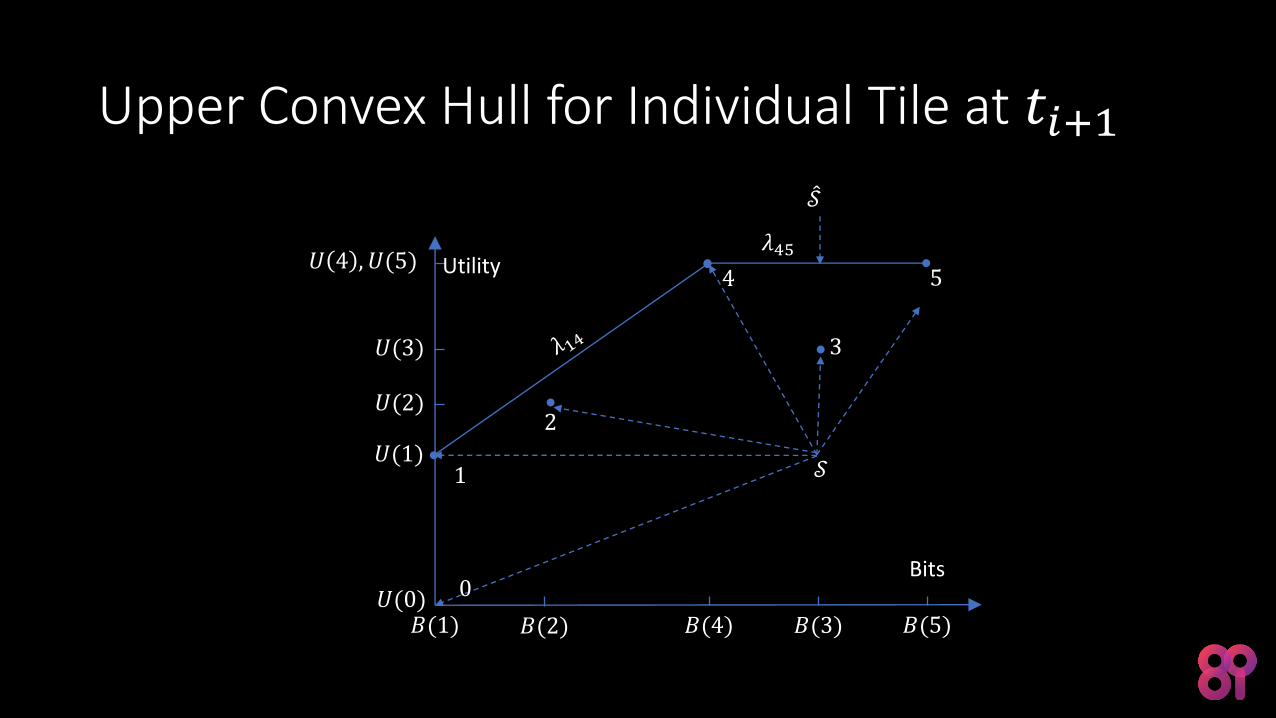
Upper Convex Hull for Individual Tile at 𝑡𝑖+1

𝐵(4)𝑈(0)

𝑈 4 , 𝑈(5)

𝑈(2)

Utility

𝒮

መ𝒮

5

3

4

2

1

0

𝐵(2) 𝐵(3) 𝐵(5)𝐵(1)

𝑈(1)

𝑈(3)

Bits

𝜆45

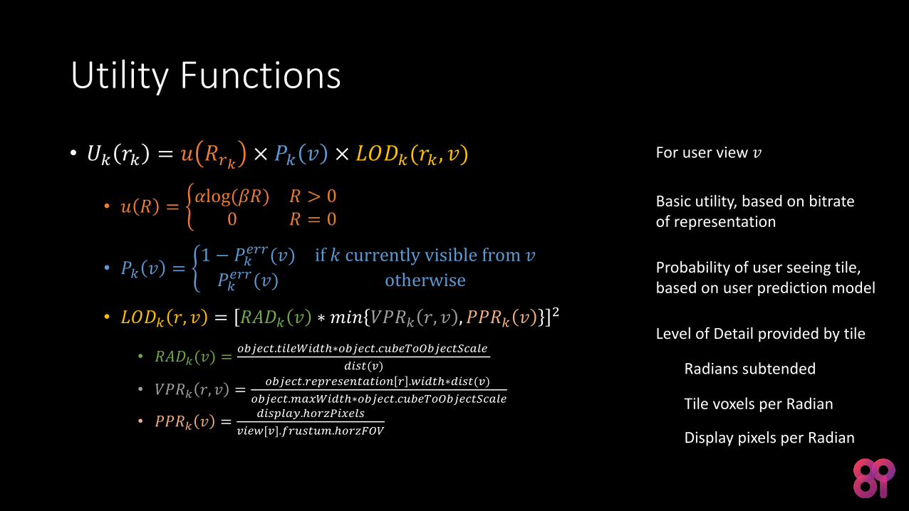
Utility Functions

• 𝑈𝑘 𝑟𝑘 = 𝑢 𝑅𝑟𝑘 × 𝑃𝑘 𝑣 × 𝐿𝑂𝐷𝑘(𝑟𝑘 , 𝑣)

• 𝑢 𝑅 = ቊ𝛼log(𝛽𝑅) 𝑅 > 0

0 𝑅 = 0

• 𝑃𝑘 𝑣 = ቊ1 − 𝑃𝑘

𝑒𝑟𝑟(𝑣) if 𝑘 currently visible from 𝑣

𝑃𝑘𝑒𝑟𝑟(𝑣) otherwise

• 𝐿𝑂𝐷𝑘 𝑟, 𝑣 = 𝑅𝐴𝐷𝑘 𝑣 ∗ 𝑚𝑖𝑛 𝑉𝑃𝑅𝑘 𝑟, 𝑣 , 𝑃𝑃𝑅𝑘 𝑣 2

• 𝑅𝐴𝐷𝑘(𝑣) =𝑜𝑏𝑗𝑒𝑐𝑡.𝑡𝑖𝑙𝑒𝑊𝑖𝑑𝑡ℎ∗𝑜𝑏𝑗𝑒𝑐𝑡.𝑐𝑢𝑏𝑒𝑇𝑜𝑂𝑏𝑗𝑒𝑐𝑡𝑆𝑐𝑎𝑙𝑒

𝑑𝑖𝑠𝑡(𝑣)

• 𝑉𝑃𝑅𝑘 𝑟, 𝑣 =𝑜𝑏𝑗𝑒𝑐𝑡.𝑟𝑒𝑝𝑟𝑒𝑠𝑒𝑛𝑡𝑎𝑡𝑖𝑜𝑛 𝑟 .𝑤𝑖𝑑𝑡ℎ∗𝑑𝑖𝑠𝑡(𝑣)

𝑜𝑏𝑗𝑒𝑐𝑡.𝑚𝑎𝑥𝑊𝑖𝑑𝑡ℎ∗𝑜𝑏𝑗𝑒𝑐𝑡.𝑐𝑢𝑏𝑒𝑇𝑜𝑂𝑏𝑗𝑒𝑐𝑡𝑆𝑐𝑎𝑙𝑒

• 𝑃𝑃𝑅𝑘 𝑣 =𝑑𝑖𝑠𝑝𝑙𝑎𝑦.ℎ𝑜𝑟𝑧𝑃𝑖𝑥𝑒𝑙𝑠

𝑣𝑖𝑒𝑤[𝑣].𝑓𝑟𝑢𝑠𝑡𝑢𝑚.ℎ𝑜𝑟𝑧𝐹𝑂𝑉

Basic utility, based on bitrate of representation

Probability of user seeing tile, based on user prediction model

Level of Detail provided by tile

Radians subtended

Tile voxels per Radian

Display pixels per Radian

For user view 𝑣

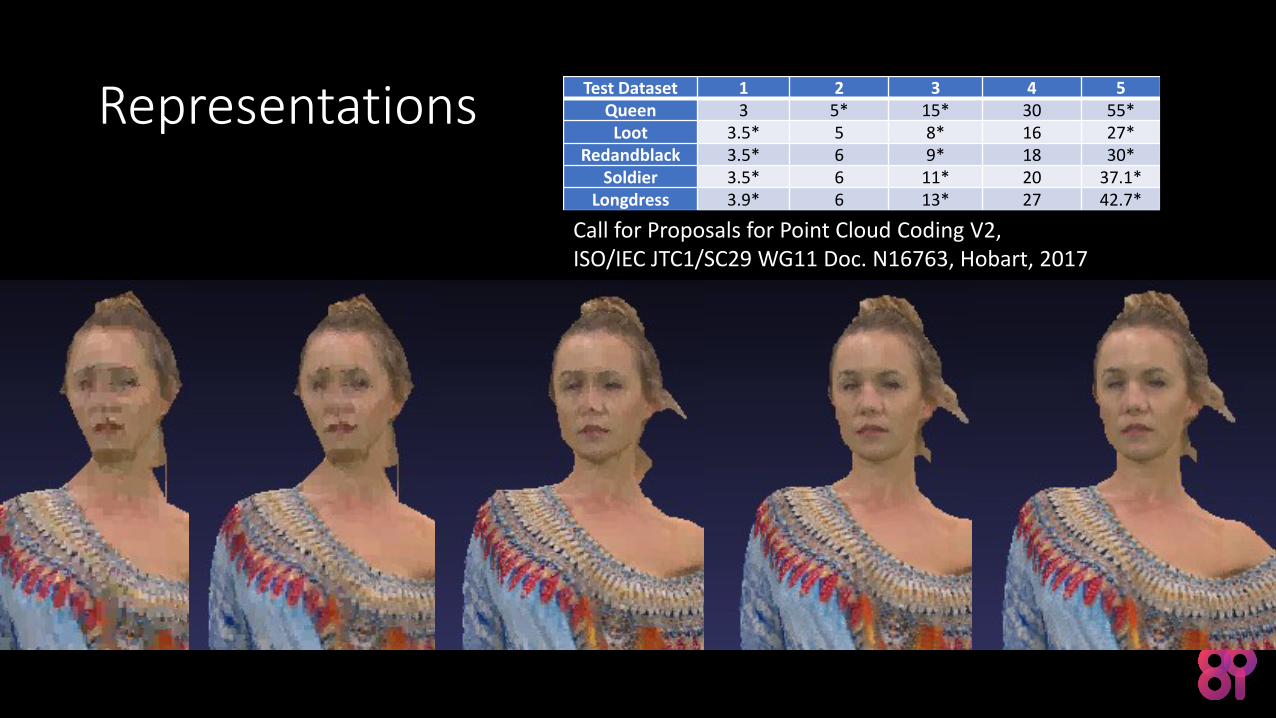
RepresentationsTest Dataset 1 2 3 4 5

Queen 3 5* 15* 30 55*Loot 3.5* 5 8* 16 27*

Redandblack 3.5* 6 9* 18 30*Soldier 3.5* 6 11* 20 37.1*

Longdress 3.9* 6 13* 27 42.7*

Call for Proposals for Point Cloud Coding V2,ISO/IEC JTC1/SC29 WG11 Doc. N16763, Hobart, 2017

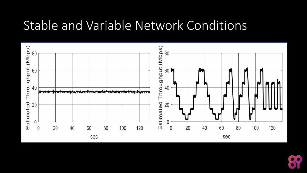
Stable and Variable Network Conditions

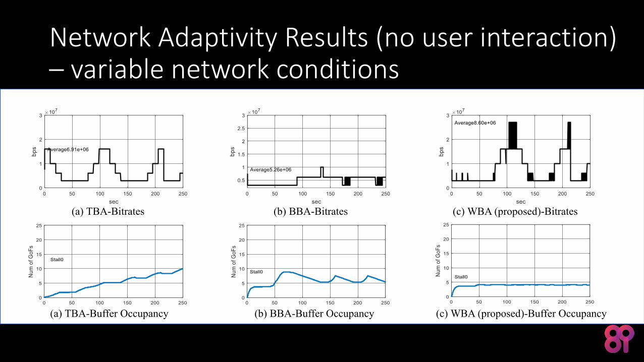
Network Adaptivity Results (no user interaction) – variable network conditions

(a) TBA-Bitrates (b) BBA-Bitrates (c) WBA (proposed)-Bitrates

(a) TBA-Buffer Occupancy (b) BBA-Buffer Occupancy (c) WBA (proposed)-Buffer Occupancy

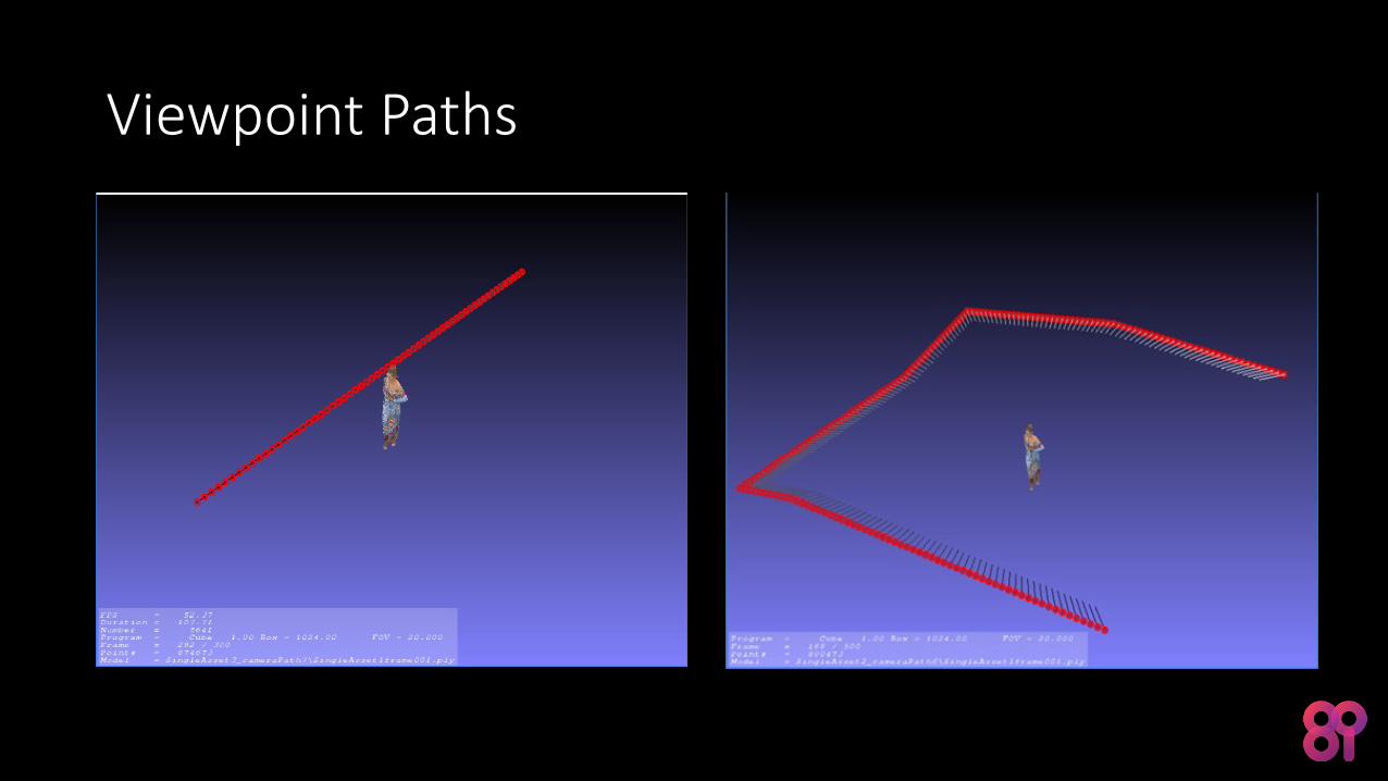
Viewpoint Paths

GoF

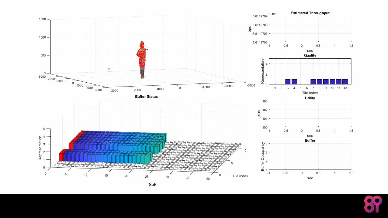
GoF

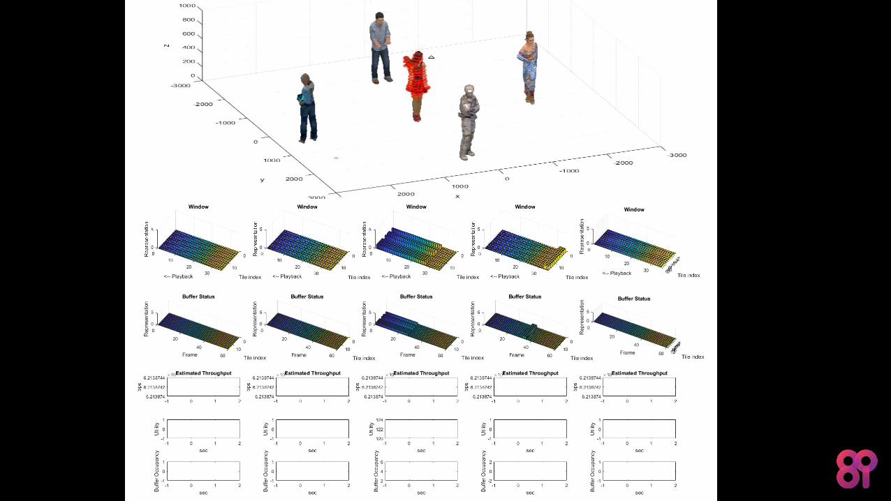
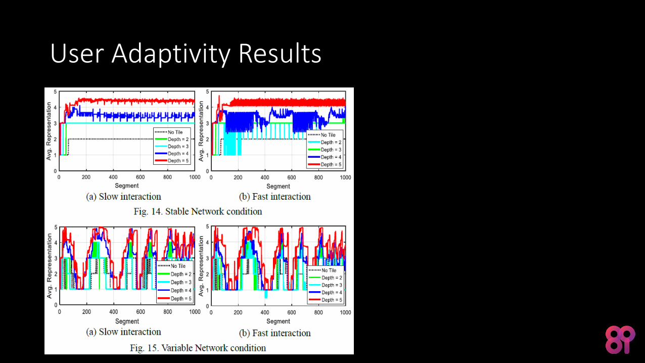
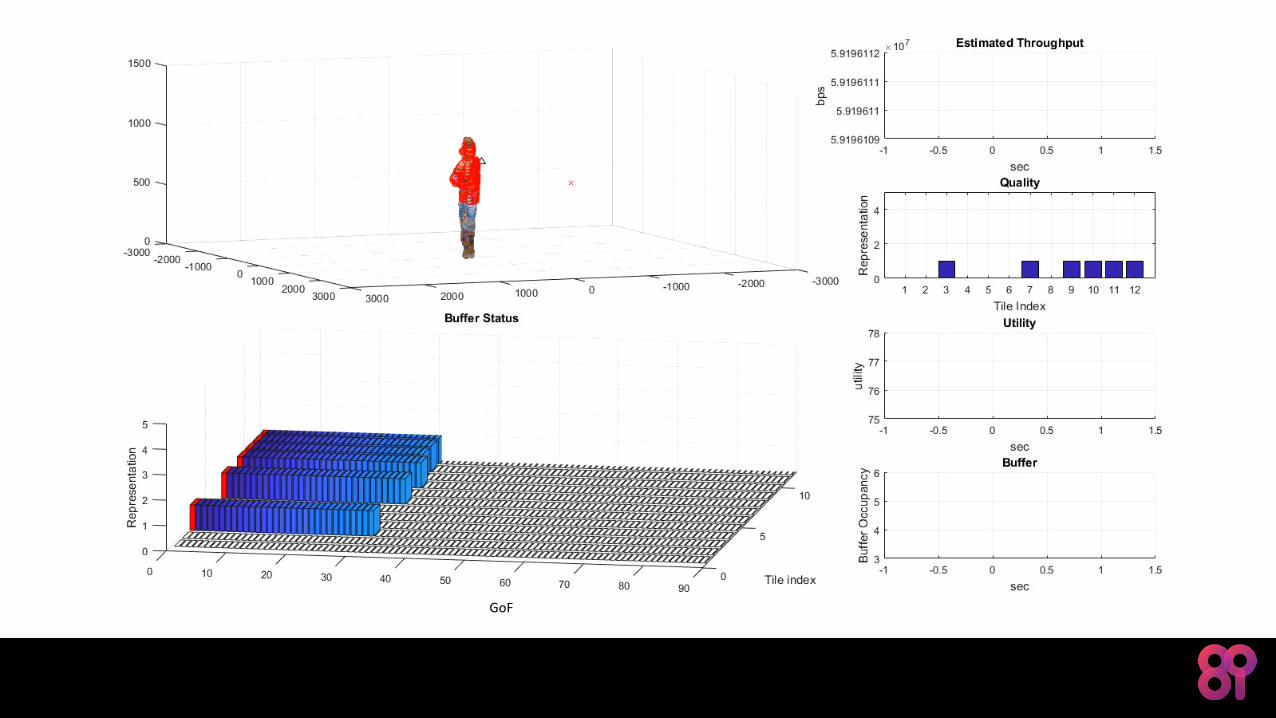
User Adaptivity Results

Conclusion: Challenges Ahead

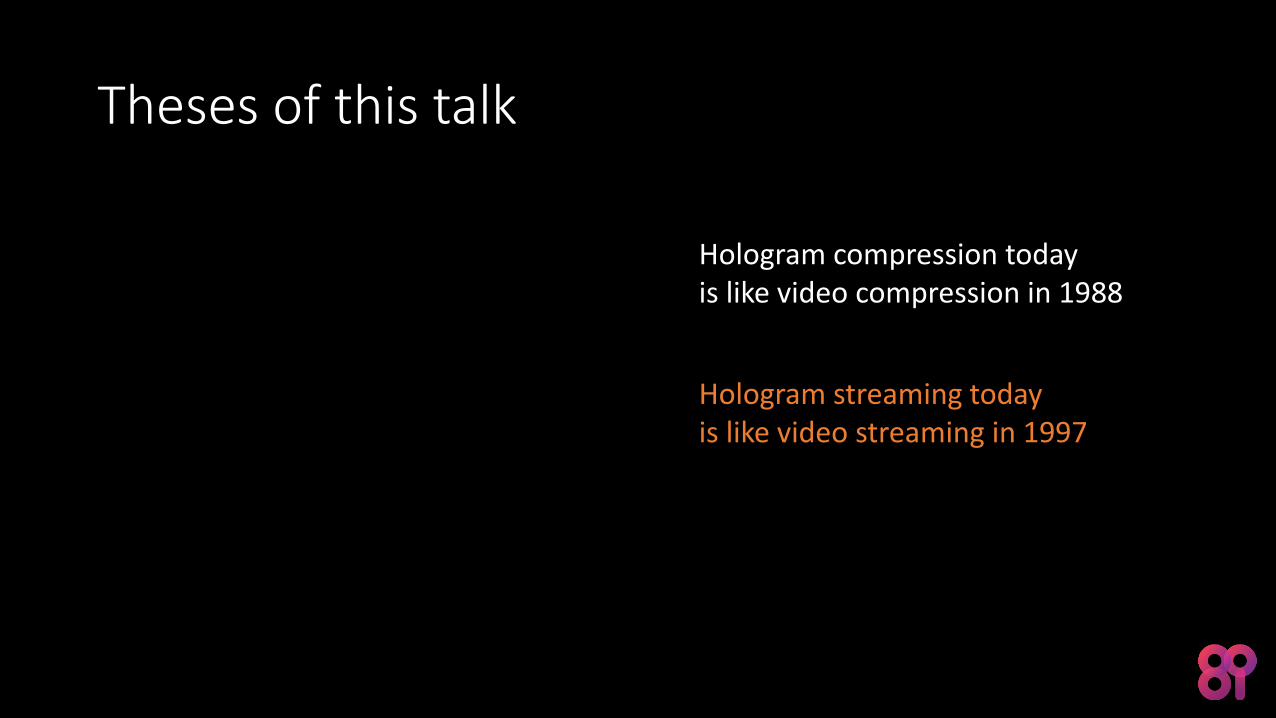
Theses of this talk

Hologram compression todayis like video compression in 1988

Hologram streaming todayis like video streaming in 1997

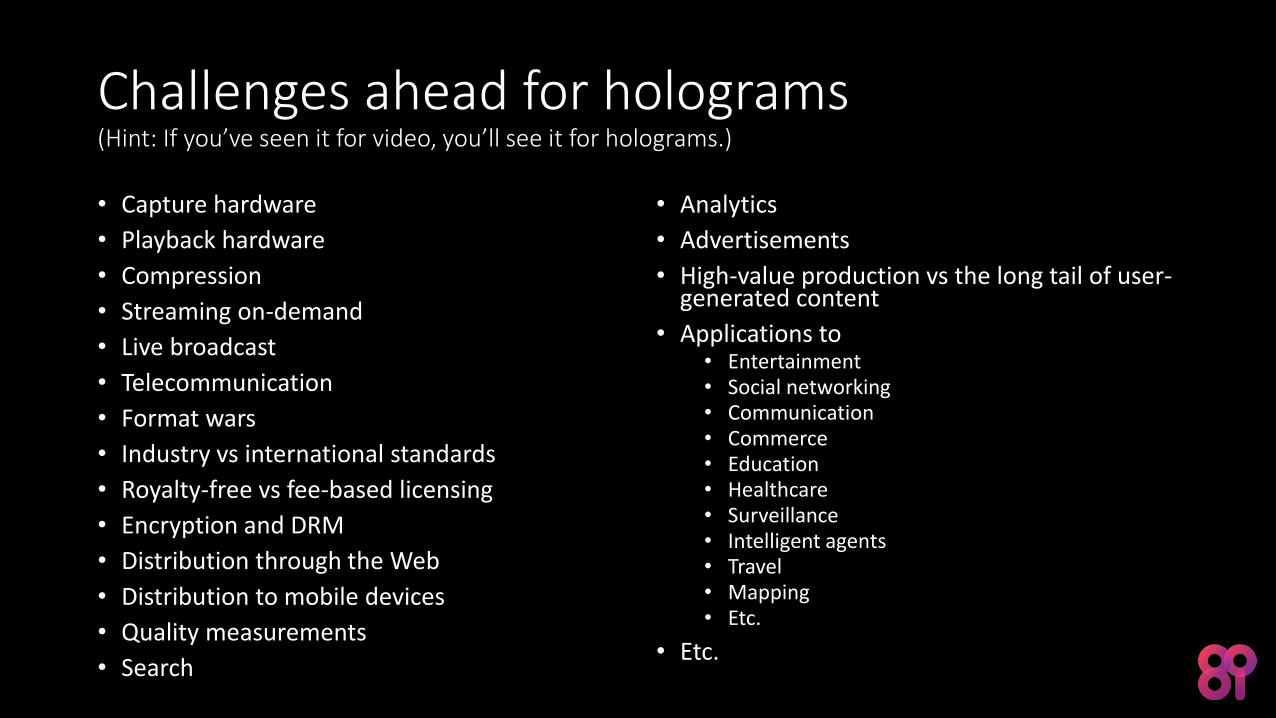
Challenges ahead for holograms(Hint: If you’ve seen it for video, you’ll see it for holograms.)

• Capture hardware

• Playback hardware

• Compression

• Streaming on-demand

• Live broadcast

• Telecommunication

• Format wars

• Industry vs international standards

• Royalty-free vs fee-based licensing

• Encryption and DRM

• Distribution through the Web

• Distribution to mobile devices

• Quality measurements

• Search

• Analytics

• Advertisements

• High-value production vs the long tail of user-generated content

• Applications to• Entertainment• Social networking• Communication• Commerce• Education• Healthcare• Surveillance• Intelligent agents• Travel• Mapping• Etc.

• Etc.

Holograms are the Next VideoPhilip A. Chou, 8i Labs, Inc.

ACM Multimedia Systems Conference13 June 2018