AIR POLLUTION AND HEALTH EFFECTS: THE CONTRIBUTION

OF TRAFFIC?The uncertainties in the full chain of traffic activity-fleet

composition-vehicle emissions-air pollution dispersion-

individual exposure- health effects

Session: Jenga - The suspense builds as the stakes get higher

Haneen Khreis, 2nd International Conference on

Transport and Health, San Jose, 13-15 June, 2016

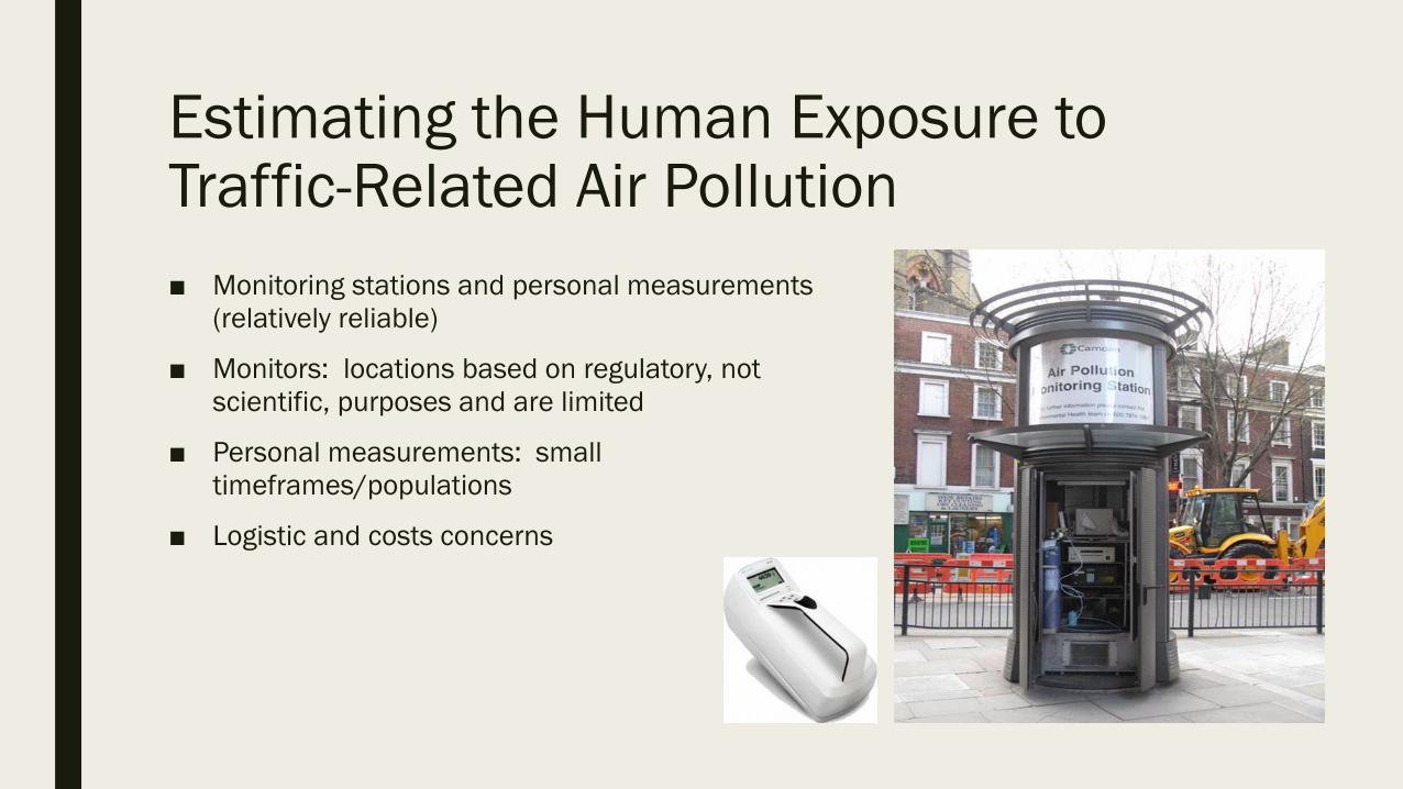
Estimating the Human Exposure to Traffic-Related Air Pollution

■ Monitoring stations and personal measurements

(relatively reliable)

■ Monitors: locations based on regulatory, not

scientific, purposes and are limited

■ Personal measurements: small

timeframes/populations

■ Logistic and costs concerns

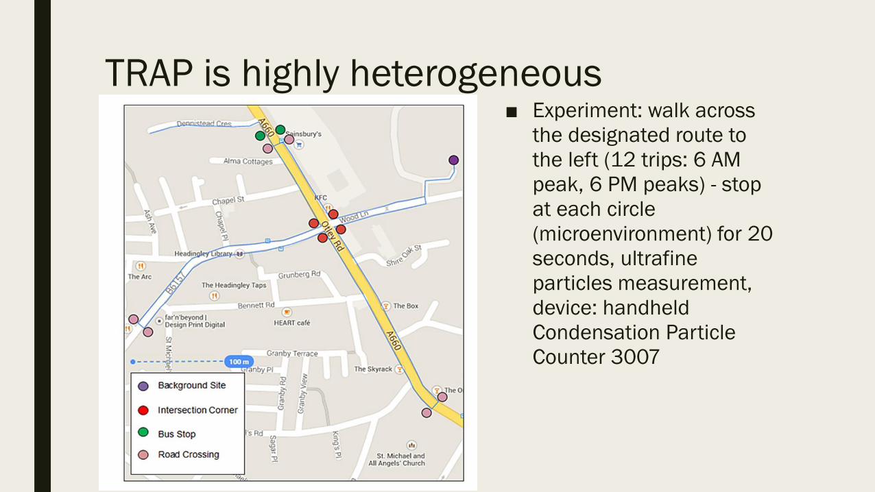
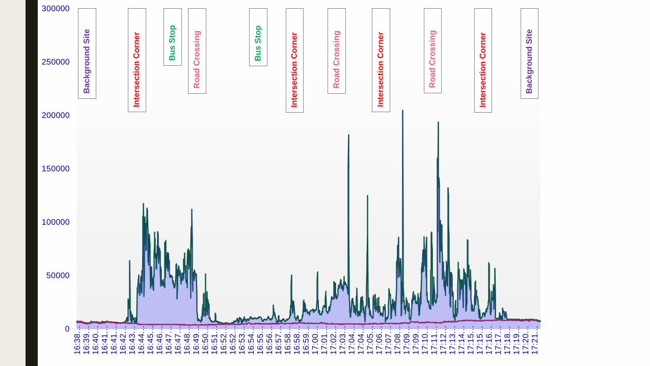
TRAP is highly heterogeneous■ Experiment: walk across

the designated route to

the left (12 trips: 6 AM

peak, 6 PM peaks) - stop

at each circle

(microenvironment) for 20

seconds, ultrafine

particles measurement,

device: handheld

Condensation Particle

Counter 3007

0

50000

100000

150000

200000

250000

300000

16

:38…

16

:39…

16

:40…

16

:41…

16

:41…

16

:42…

16

:43…

16

:44…

16

:45…

16

:46…

16

:47…

16

:47…

16

:48…

16

:49…

16

:50…

16

:51…

16

:52…

16

:52…

16

:53…

16

:54…

16

:55…

16

:56…

16

:57…

16

:58…

16

:58…

16

:59…

17

:00…

17

:01…

17

:02…

17

:03…

17

:04…

17

:04…

17

:05…

17

:06…

17

:07…

17

:08…

17

:09…

17

:09…

17

:10…

17

:11…

17

:12…

17

:13…

17

:14…

17

:15…

17

:15…

17

:16…

17

:17…

17

:18…

17

:19…

17

:20…

17

:21…

Bac

kg

rou

nd

Sit

e

Bac

kg

rou

nd

Sit

e

Inte

rse

cti

on

Co

rne

r

Bu

sS

top

Ro

ad

Cro

ss

ing

Bu

sS

top

Inte

rse

cti

on

Co

rne

r

Ro

ad

Cro

ss

ing

Inte

rse

cti

on

Co

rne

r

Inte

rse

cti

on

Co

rne

r

Ro

ad

Cro

ss

ing

Estimating the Human Exposure to Traffic-Related Air Pollution

■ Surrogates for Human Exposure

– Proximity to ‘major roads’.

– Vehicles counts (& composition).

– Land Use Regression models.

– Geostatistical interpolation (GIS).

– Hybrid models (mixture, activity diaries, home monitors, indices)

(2).

– And dispersion models…….

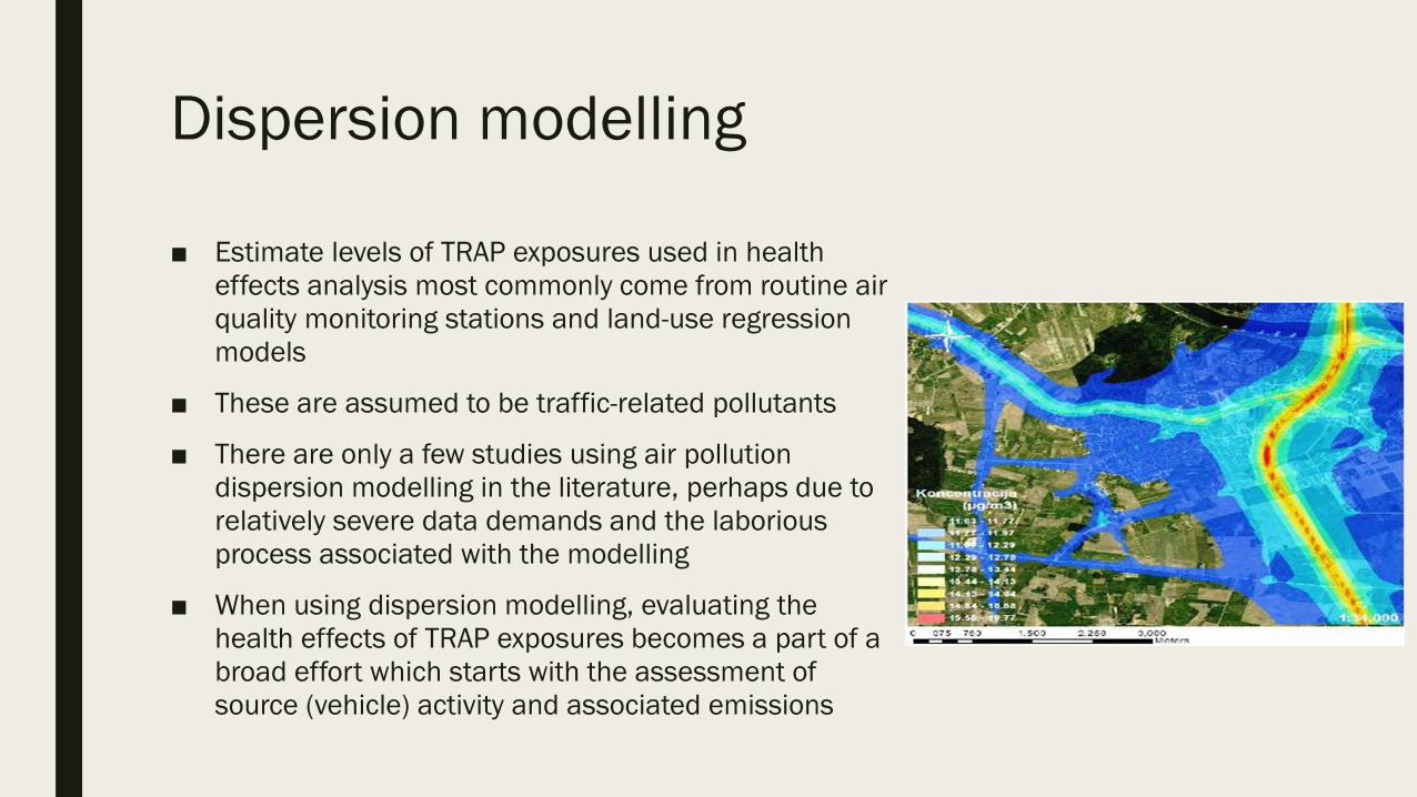
Dispersion modelling

■ Estimate levels of TRAP exposures used in health

effects analysis most commonly come from routine air

quality monitoring stations and land-use regression

models

■ These are assumed to be traffic-related pollutants

■ There are only a few studies using air pollution

dispersion modelling in the literature, perhaps due to

relatively severe data demands and the laborious

process associated with the modelling

■ When using dispersion modelling, evaluating the

health effects of TRAP exposures becomes a part of a

broad effort which starts with the assessment of

source (vehicle) activity and associated emissions

Air pollution: the contribution of traffic?

Compliance,

effectiveness

Atmospheric transport,

chemical transformation,

and deposition

Human time-activity in relation

to indoor and outdoor air quality;

Uptake, deposition, clearance, retention

Susceptibility factors;

mechanisms of damage

and repair, health outcomes

Transport

policy

Emissions

Ambient air

quality

Exposure/

dose

Human

healthHEI, 2003

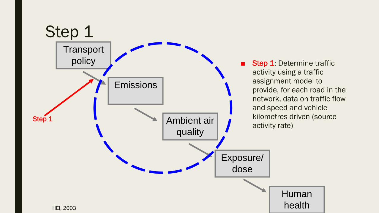
Step 1

■ Step 1: Determine traffic

activity using a traffic

assignment model to

provide, for each road in the

network, data on traffic flow

and speed and vehicle

kilometres driven (source

activity rate)

Transport

policy

Emissions

Ambient air

quality

Exposure/

dose

Human

healthHEI, 2003

Step 1

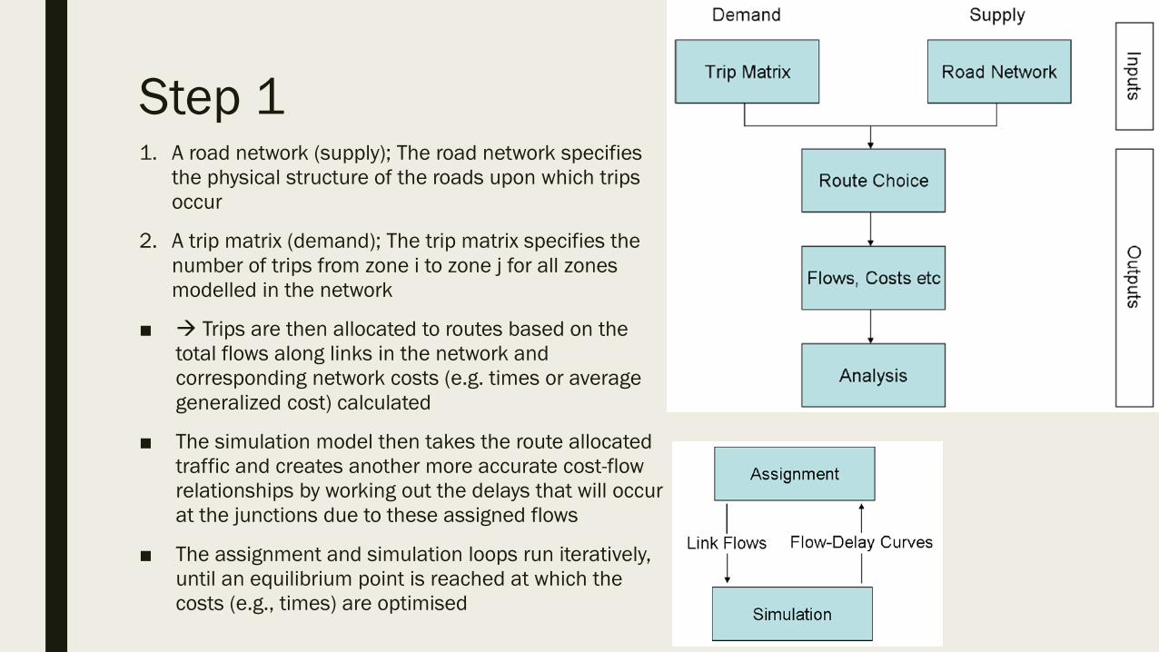
Step 11. A road network (supply); The road network specifies

the physical structure of the roads upon which trips

occur

2. A trip matrix (demand); The trip matrix specifies the

number of trips from zone i to zone j for all zones

modelled in the network

■ Trips are then allocated to routes based on the

total flows along links in the network and

corresponding network costs (e.g. times or average

generalized cost) calculated

■ The simulation model then takes the route allocated

traffic and creates another more accurate cost-flow

relationships by working out the delays that will occur

at the junctions due to these assigned flows

■ The assignment and simulation loops run iteratively,

until an equilibrium point is reached at which the

costs (e.g., times) are optimised

Step 1

Step 1

■ Outputs

– Traffic average speed (AM peak hour, Inter-peak hour, PM peak hour)

– Traffic flow (passenger car units/hour)

■ Acceptance criteria (in comparison to real life):

■ Traffic flow: G𝐸𝐻 =2(𝑀−𝐶)2

𝑀+𝐶

– GEH of less than ‘5.0’ is considered a good match between the modelled and

observed hourly volumes, and 85% of the volumes in a traffic model should

achieve this criteria (240 links)

■ Traffic speed (52 journeys)

– Average difference between modelled and observed journey times within 15%

for all time periods

Modelled journey times are consistently faster than observed, in all time periods,

suggesting that congestion is under-represented in the models

Time

period

Test

1 2 3 4 5

AM 40% 77% 40% 88% 73%

IP 46% 89% 46% 95% 78%

PM 42% 73% 42% 82% 63%

Conclusions

■ SATURN is a static equilibrium model, intended to provide long-run estimates of vehicle flow, rather than a snapshot of what happened on a particular day

■ Does not consider the effect of acceleration and deceleration at junctions, and has a uniform emission through a junction based on average speed

■ Validation is difficult because the cost of obtaining network wide, long-run observed counts is prohibitive

■ And because there is usually significant uncertainty in the observed count data

■ Validation is conducted at the project scale

■ Sensitivity testing on the model show that the model is remarkably stable at the aggregate level, but less so at the link level

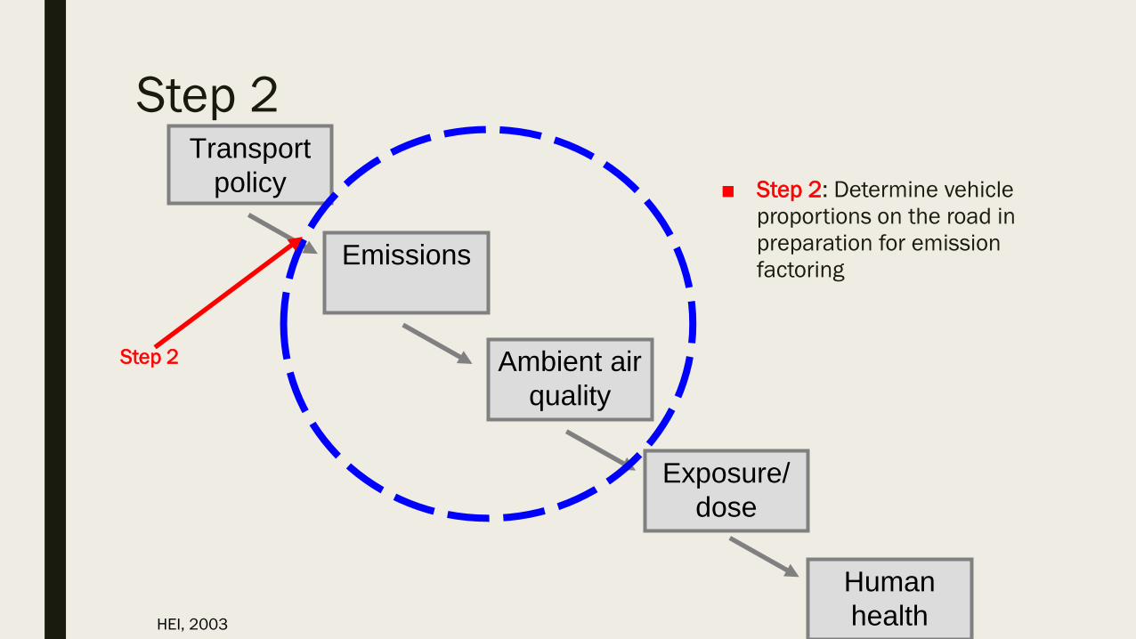
Step 2

■ Step 2: Determine vehicle

proportions on the road in

preparation for emission

factoring

Transport

policy

Emissions

Ambient air

quality

Exposure/

dose

Human

healthHEI, 2003

Step 2

Step 2

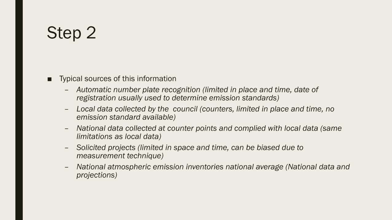
■ Typical sources of this information

– Automatic number plate recognition (limited in place and time, date of registration usually used to determine emission standards)

– Local data collected by the council (counters, limited in place and time, no emission standard available)

– National data collected at counter points and complied with local data (same limitations as local data)

– Solicited projects (limited in space and time, can be biased due to measurement technique)

– National atmospheric emission inventories national average (National data and projections)

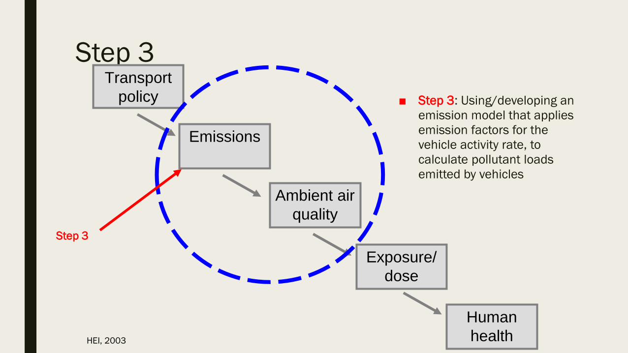
Step 3

■ Step 3: Using/developing an

emission model that applies

emission factors for the

vehicle activity rate, to

calculate pollutant loads

emitted by vehicles

Transport

policy

Emissions

Ambient air

quality

Exposure/

dose

Human

healthHEI, 2003

Step 3

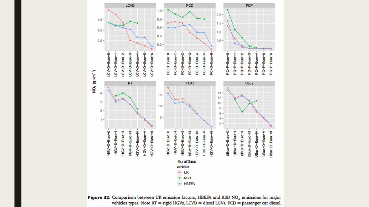
Step 3

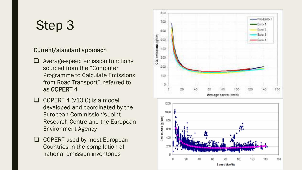
Current/standard approach

Average-speed emission functions

sourced from the “Computer

Programme to Calculate Emissions

from Road Transport”, referred to

as COPERT 4

COPERT 4 (v10.0) is a model

developed and coordinated by the

European Commission's Joint

Research Centre and the European

Environment Agency

COPERT used by most European

Countries in the compilation of

national emission inventories

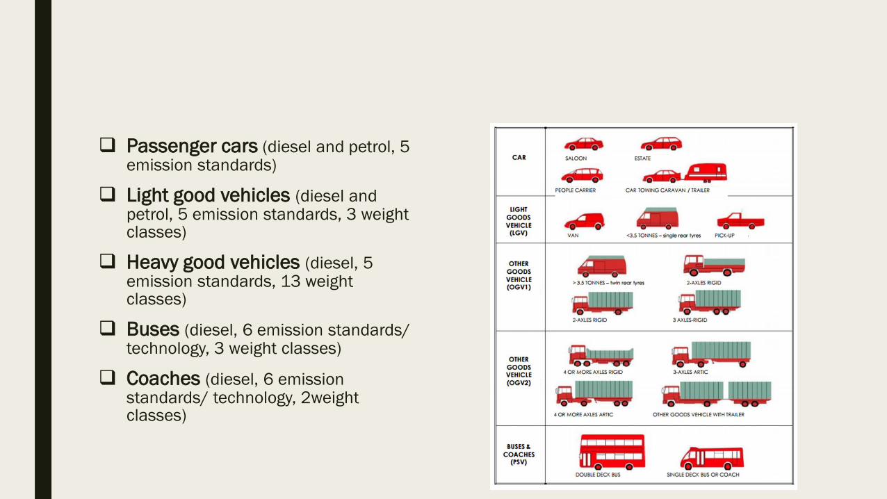
Passenger cars (diesel and petrol, 5 emission standards)

Light good vehicles (diesel and petrol, 5 emission standards, 3 weight classes)

Heavy good vehicles (diesel, 5 emission standards, 13 weight classes)

Buses (diesel, 6 emission standards/ technology, 3 weight classes)

Coaches (diesel, 6 emission standards/ technology, 2weight classes)

Step 3

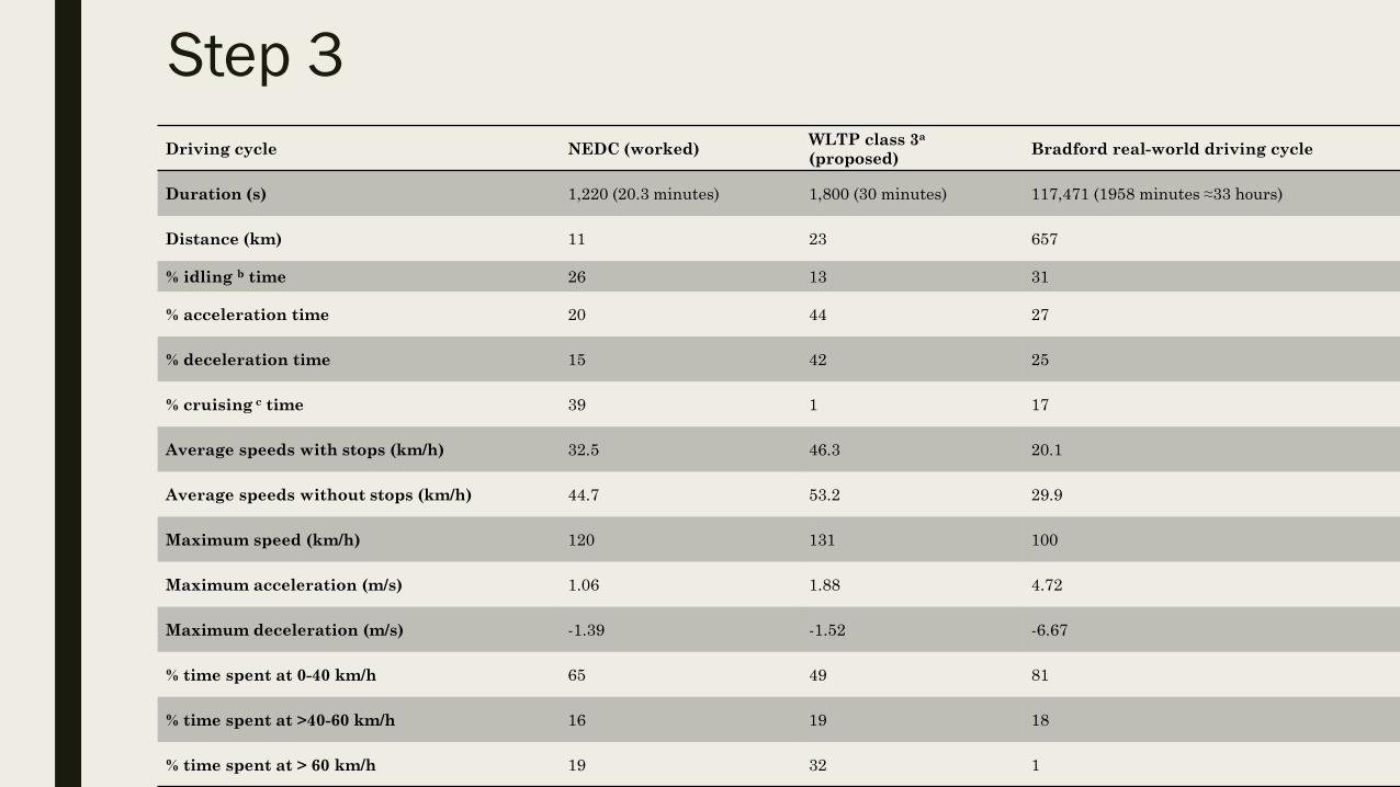
Driving cycle NEDC (worked)WLTP class 3a

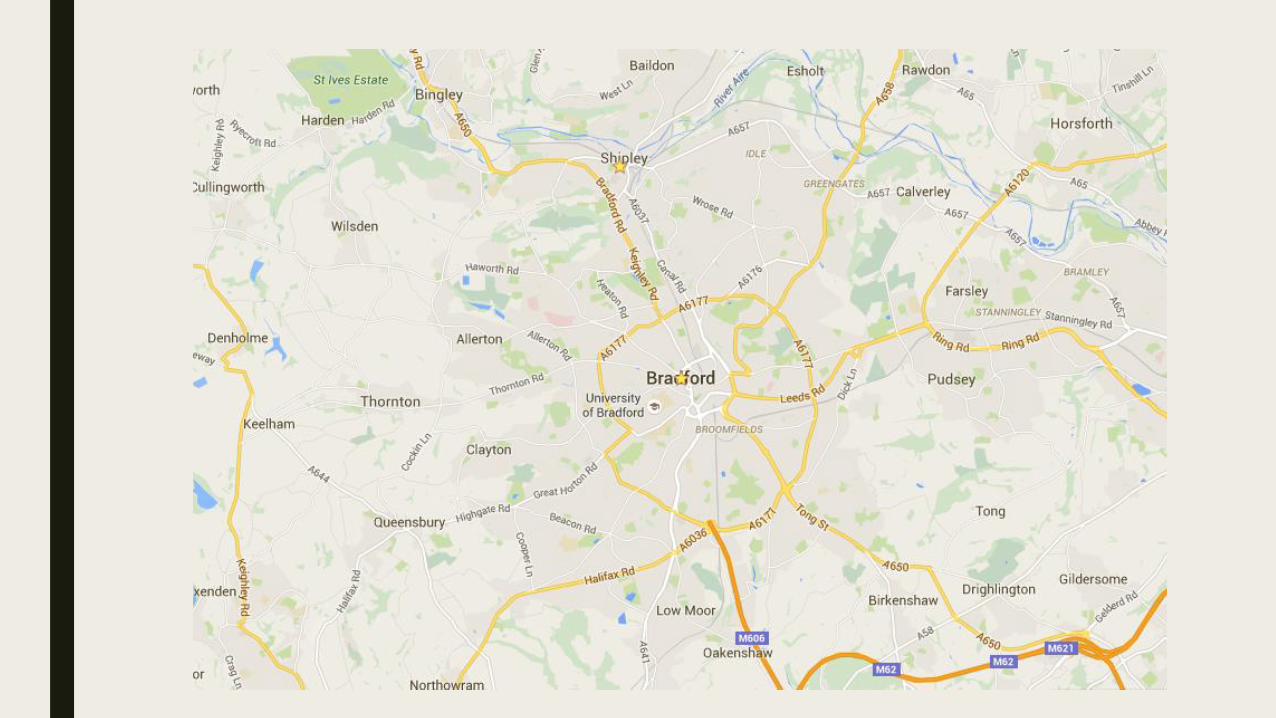
(proposed)Bradford real-world driving cycle

Duration (s) 1,220 (20.3 minutes) 1,800 (30 minutes) 117,471 (1958 minutes ≈33 hours)

Distance (km) 11 23 657

% idling b time 26 13 31

% acceleration time 20 44 27

% deceleration time 15 42 25

% cruising c time 39 1 17

Average speeds with stops (km/h) 32.5 46.3 20.1

Average speeds without stops (km/h) 44.7 53.2 29.9

Maximum speed (km/h) 120 131 100

Maximum acceleration (m/s) 1.06 1.88 4.72

Maximum deceleration (m/s) -1.39 -1.52 -6.67

% time spent at 0-40 km/h 65 49 81

% time spent at >40-60 km/h 16 19 18

% time spent at > 60 km/h 19 32 1

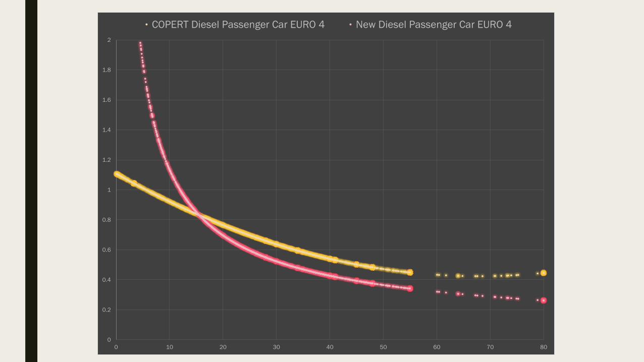
0

0.2

0.4

0.6

0.8

1

1.2

1.4

1.6

1.8

2

0 10 20 30 40 50 60 70 80

COPERT Diesel Passenger Car EURO 4 New Diesel Passenger Car EURO 4

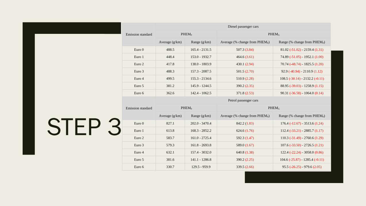
Emission standard

Diesel passenger cars

PHEM0 PHEMG

Average (g/km) Range (g/km) Average (% change from PHEM0) Range (% change from PHEM0)

Euro 0 488.5 165.4 - 2131.5 507.3 (3.84) 81.02 (-51.02) - 2159.4 (1.31)

Euro 1 448.4 153.0 - 1932.7 464.6 (3.61) 74.89 (-51.05) - 1952.1 (1.00)

Euro 2 417.8 138.0 - 1803.9 430.1 (2.94) 70.74 (-48.74) - 1825.5 (1.20)

Euro 3 488.3 157.3 - 2087.5 501.5 (2.70) 92.9 (-40.94) - 2110.9 (1.12)

Euro 4 499.5 155.3 - 2134.6 510.9 (2.28) 108.5 (-30.14) - 2132.2 (-0.11)

Euro 5 381.2 145.9 - 1244.5 390.2 (2.35) 88.95 (-39.03) - 1258.9 (1.15)

Euro 6 362.6 142.4 - 1062.5 371.8 (2.53) 90.31 (-36.58) - 1064.0 (0.14)

Emission standard

Petrol passenger cars

PHEM0 PHEMG

Average (g/km) Range (g/km) Average (% change from PHEM0) Range (% change from PHEM0)

Euro 0 827.1 202.0 - 3470.4 842.2 (1.83) 176.4 (-12.67) - 3513.6 (1.24)

Euro 1 613.8 168.3 - 2852.2 624.6 (1.76) 112.4 (-33.21) - 2885.7 (1.17)

Euro 2 583.7 161.0 - 2725.4 592.3 (1.47) 110.3 (-31.49) - 2760.6 (1.29)

Euro 3 579.3 161.8 - 2693.8 589.0 (1.67) 107.6 (-33.50) - 2726.5 (1.21)

Euro 4 632.1 157.4 - 3032.0 640.8 (1.38) 122.4 (-22.24) - 3058.0 (0.86)

Euro 5 381.6 141.1 - 1286.8 390.2 (2.25) 104.6 (-25.87) - 1285.4 (-0.11)

Euro 6 330.7 129.5 - 959.9 339.5 (2.66) 95.5 (-26.25) - 979.6 (2.05)

STEP 3

Conclusions ■ Current emission factors unreliable, especially at lower speeds

■ There is a lack of clarity about the underlying data?

■ Emission factors are based on limited observations, which differ from the activities to which

they are applied

■ Using a small vehicle sample to represent a vehicle fleet of millions

■ Driving cycle not representative

■ Not considering all actual environmental conditions in emission estimation

■ Validation of urban emission models through comparison of observed–predicted values has

never been done, as it is not feasible to monitor emissions from all vehicles travelling on a

road

■ Neither is it possible to accurately quantify uncertainties in emissions due to the complex and

varied nature of the data and calculations associated with emission estimation

Step 4

■ Step 4: Using a dispersion

model to simulate emissions

dispersion across study area

Transport

policy

Emissions

Ambient air

quality

Exposure/

dose

Human

healthHEI, 2003

Step 4

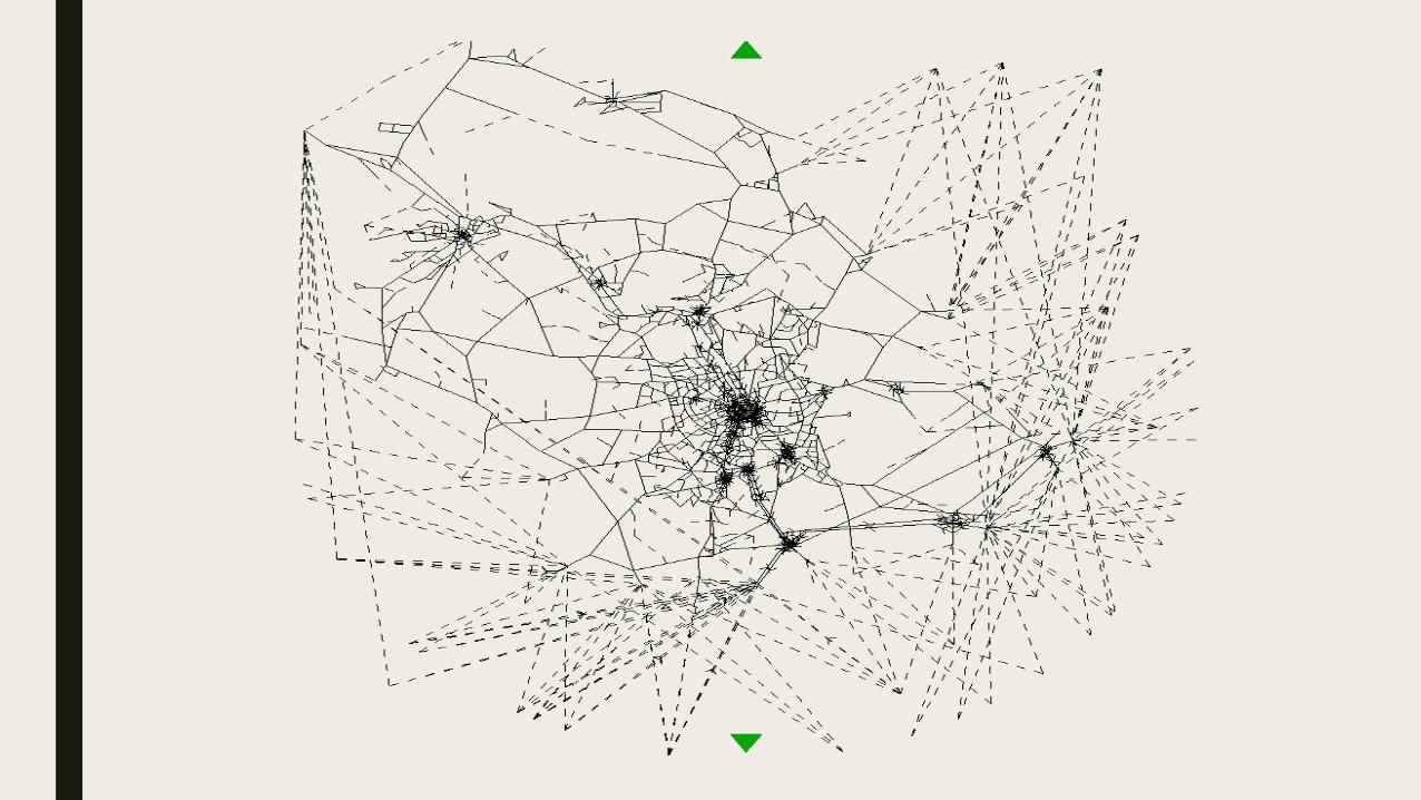
STEP 4Combine mobile source

emissions with

stationary source

emissions (from

industries, etc.)

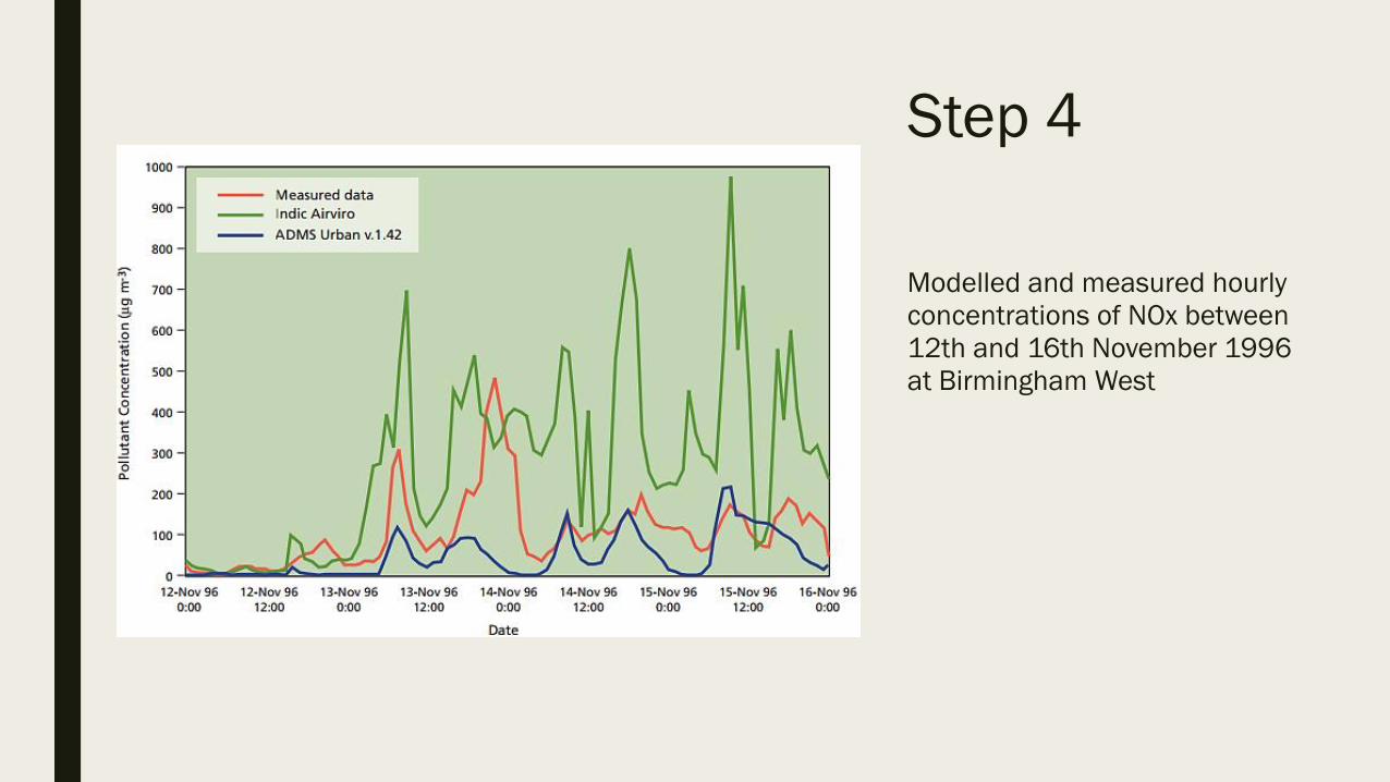
Step 4

Modelled and measured hourly

concentrations of NOx between

12th and 16th November 1996

at Birmingham West

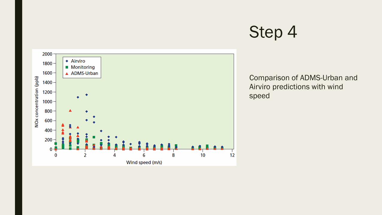
Step 4

Comparison of ADMS-Urban and

Airviro predictions with wind

speed

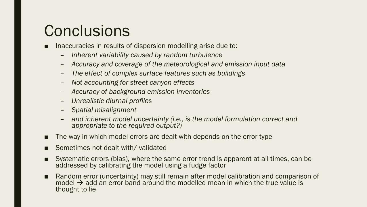
Conclusions■ Inaccuracies in results of dispersion modelling arise due to:

– Inherent variability caused by random turbulence

– Accuracy and coverage of the meteorological and emission input data

– The effect of complex surface features such as buildings

– Not accounting for street canyon effects

– Accuracy of background emission inventories

– Unrealistic diurnal profiles

– Spatial misalignment

– and inherent model uncertainty (i.e., is the model formulation correct and appropriate to the required output?)

■ The way in which model errors are dealt with depends on the error type

■ Sometimes not dealt with/ validated

■ Systematic errors (bias), where the same error trend is apparent at all times, can be addressed by calibrating the model using a fudge factor

■ Random error (uncertainty) may still remain after model calibration and comparison of model add an error band around the modelled mean in which the true value is thought to lie

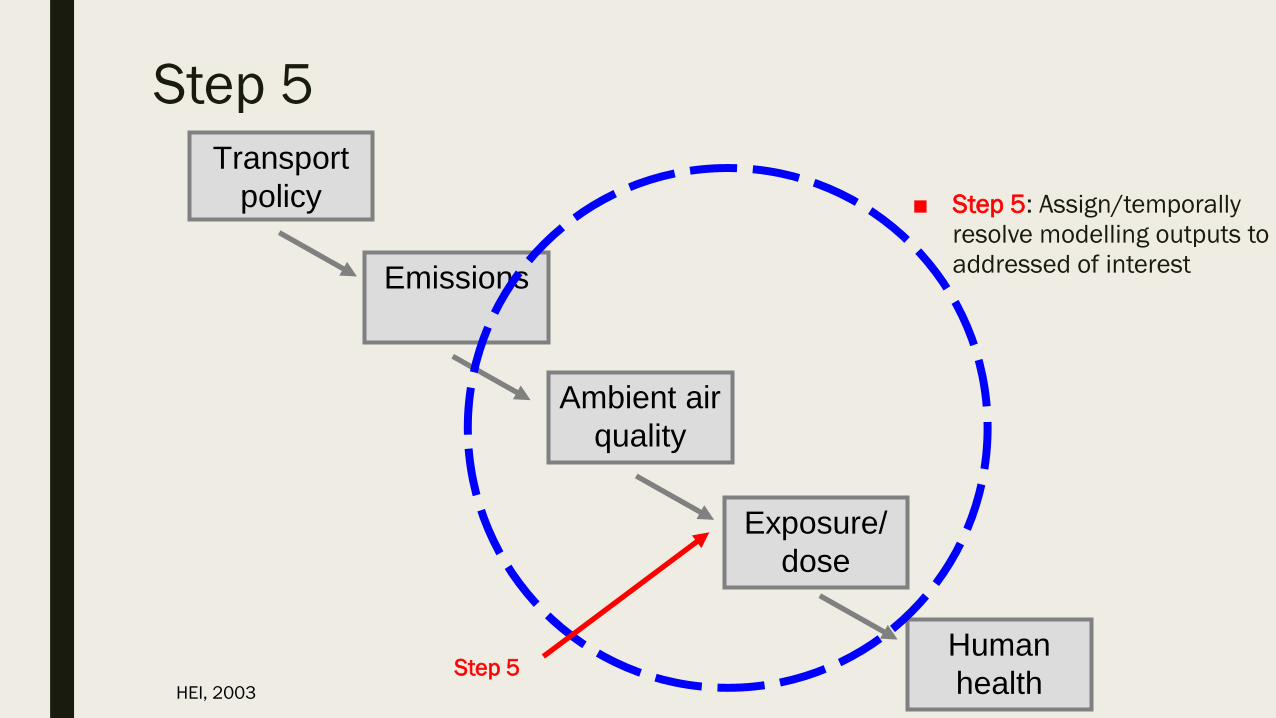
Step 5

■ Step 5: Assign/temporally

resolve modelling outputs to

addressed of interest

Transport

policy

Emissions

Ambient air

quality

Exposure/

dose

Human

healthHEI, 2003

Step 5

Step 5

– Home location Standard

– Work/study location Sometimes

– Commute Rarely

– Elsewhere Rarely

■ E.g. (systematic review of 38 studies ) TRAP exposures almost exclusively assigned based on the participants’ residential addresses (35 studies – 3 looked at school and daycare centres)

■ Only 8 recent studies, 5 of which published after 2014, considered children’s mobility at ages when exposure at the residential address is less relevant and assigned time-weighted TRAP exposures at daycare-centres and schools alongside residence

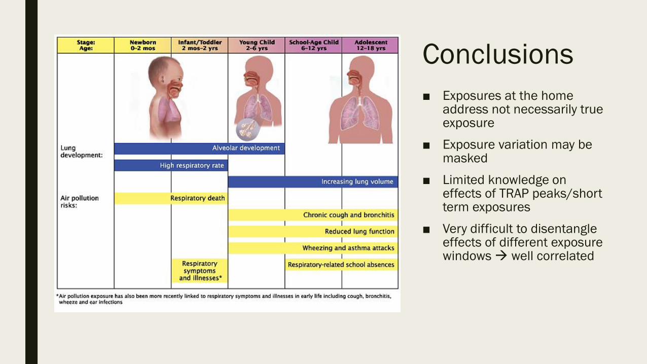
Conclusions

■ Exposures at the home address not necessarily true exposure

■ Exposure variation may be masked

■ Limited knowledge on effects of TRAP peaks/short term exposures

■ Very difficult to disentangle effects of different exposure windows well correlated

Step 6

■ Step 6: Assess associations

between exposures and

health outcomes

Transport

policy

Emissions

Ambient air

quality

Exposure/

dose

Human

healthHEI, 2003Step 6

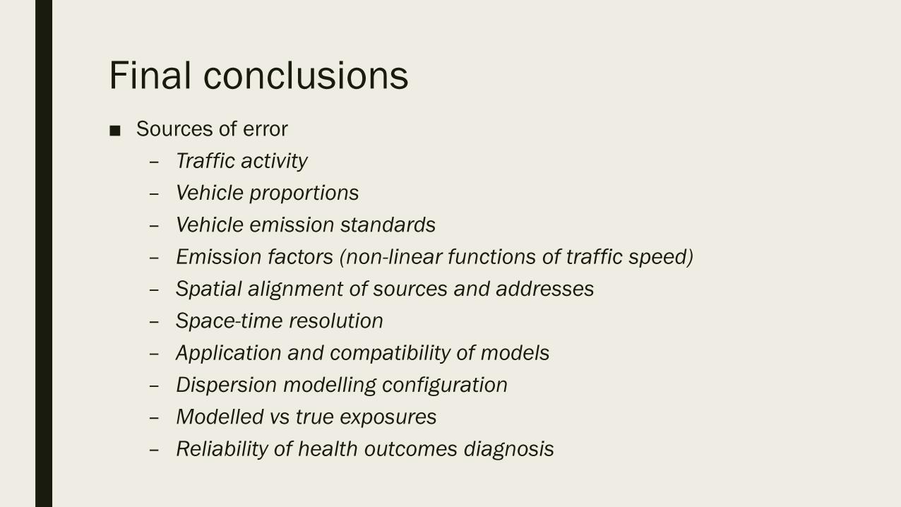
Final conclusions

■ Sources of error

– Traffic activity

– Vehicle proportions

– Vehicle emission standards

– Emission factors (non-linear functions of traffic speed)

– Spatial alignment of sources and addresses

– Space-time resolution

– Application and compatibility of models

– Dispersion modelling configuration

– Modelled vs true exposures

– Reliability of health outcomes diagnosis

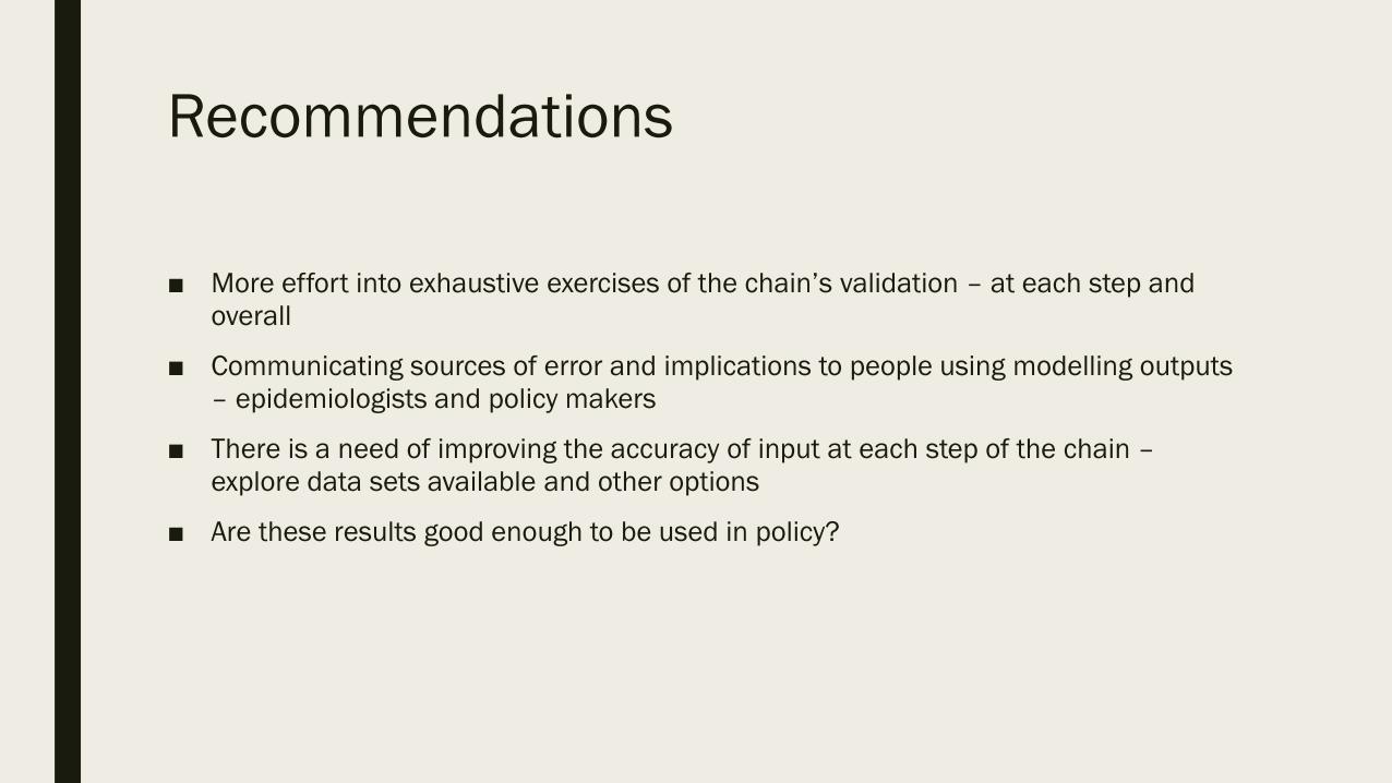
Recommendations

■ More effort into exhaustive exercises of the chain’s validation – at each step and

overall

■ Communicating sources of error and implications to people using modelling outputs

– epidemiologists and policy makers

■ There is a need of improving the accuracy of input at each step of the chain –

explore data sets available and other options

■ Are these results good enough to be used in policy?