1

IAC-09-E4.2.4

HISTORICAL EVOLUTION OF SPACE SYSTEMS

Svenja Stellmann

University of Applied Sciences Bremen, Germany

Svenja@Stellmann.info

Daniel Schubert, Andre Weiss DLR German Aerospace Center, Bremen, Germany

Daniel.Schubert@dlr.de, Andre.Weiss@dlr.de

ABSTRACT

Since the launch of Sputnik in 1957, thousands of satellites and space probes have been sent into space. The typical

spacecraft subsystems were subject of steady technology improvements during the last five decades, which led to

many changes in design and layout.

Darwin taught us that biological systems adapt and improve by a process of natural selection, known to us as evolu-

tion. The question rises if similar forces lead to an evolution within the technical world of spacecraft engineering?

Can technical systems evolve over time so that one can call it technology evolution? Influences like technology S-

curves, trend analysis, disruptive technology innovations, technology maps, space system failure studies and differ-

ent subsystem development ratios are only a few factors that need to be considered in order to answer the question.

The results presented in this paper are based on the intensive research and analysis of a specially created database,

fed from several (smaller) databases containing technical specifications (mass & power budgets) of hundreds of

spacecrafts. The focus was set on exploration systems, which were analysed with different regression and correla-

tion algorithms in order to reveal specific trends of a spacecraft subsystem as a function of time.

Analysing the evolution of spacecraft systems has two main purposes: To give technical guidance for future space-

craft designs (performed e.g. in Concurrent Engineering studies) as well as to establish a system to evaluate which

technologies are worth investing in, depending on their overall technology maturity. The paper was prepared within

the Department for System Analysis Space Segments at the Institute of Space Systems (German Aerospace Center -

DLR) in co-operation with the University of Applied Sciences, Bremen (Germany).

INTRODUCTION

The past 50 years have seen rapid increase in the

speed of progress in various technological fields. The

development and improvement of devices, like televi-

sion, telephone, cars, computers or mobile phones is

very familiar to all of us. Every day we benefit from

the improvements engineers and scientists have

achieved. But how did such a technological system

evolve? How is progress achieved and assured? And

where will it lead us eventually? How was the techni-

cal development of one individual subsystem carried

out? Which principles (objectives and requirements)

were crucial during the development? Are there tem-

poral or causal relations between the individual sub-

systems in term of technology evolution? Were there

technology leaps in the evolution of spacecraft and

their subsystems? Can future trend for space flight be

detected, and hence can guidelines be educed for a

successful technology management from them? To

frame an answer, a general literature research on tech-

nology development and evolution, as well as on

analysis of technology evolutions in space flight, is

necessary.

TECHNOLOGY EVOLUTION

Natural selection is the driving force of evolution in

nature. This theory was founded by the natural scien-

tist Charles Darwin in 1859 with his book “The Origin

of Species”. [1], [2] He argues that this natural selec-

tion is triggered by randomly appearing attributes or

characteristics depending, which give an advantage to

the life form or species they appear in. This advantage

is dependent on the environmental conditions the

organism is living in. It is given onwards to the next

generations, by which the chance of survival of that

given species is increased.

Hill argues that life itself laid the basis for further

evolution through technology. [3] Because human

abilities are limited to a certain level, the technological

progress continues the natural evolution to overcome

these limitations. Hill underlines this assumption by

providing the example of the human eye, which, al-

2

though being a very powerful instrument, is limited in

its ability to see objects very far away (e.g. other pla-

nets) or very small objects (e.g. atoms). In order to

overcome this natural limitation the technological

evolution has developed devices to help improving the

human vision.

Today however, the aim of a new technology is usual-

ly defined before it is being developed and the given

resources are used efficiently to achieve the given

goal.

Generally speaking, technological progress is directed

towards an ideal state as Hill describes it. [3] A good

way to reach this ideality, or to get at least near it, is

the orientation on similar systems in nature. Such

systems went past a development lasting millions of

years through biological evolution and are usually

very close to an ideal design, if not having reached it.

Altschuller defines an ideal system where attributes

such as mass, volume and surface approaches zero,

while the ability to fulfil a certain performance is not

reduced. [4] But this being only a general rule, does

not explain how technological progress is systemati-

cally achieved.

Hill gives a good example of technological enhance-

ment by increasing the degree of efficiency, referring

to the development of the steam-engine. The machine

was enhanced by James Watt, who identified weak-

nesses in the steam-engine design by Newcomen. The

redesign resulted in an increased performance with

less energy consumption, hence an increase of the

degree of efficiency. [3]

The example illustrates that an increase of the degree

of efficiency is achieved by further developing an

existing design. This is an important characteristic of

technological evolution. There has to be some kind of

source it is based on. The most basic source being a

good idea, as we heard before. Hill calls the enhance-

ment of an existing design, quantitative enhancements.

But even if the degree of efficiency of the steam-

engine would have been enhanced a hundred times, it

would still be based on the same technical principle of

using pressurized steam as a working medium. A

qualitative enhancement, as Hill describes it, is

achieved when a new principle is being introduced. In

the case of the steam-engine the qualitative enhance-

ment was achieved when, for example, the electro-

dynamic principle of the electric motor was intro-

duced. The development from the quantitative en-

hancements of the efficiency of the steam-engine to

the qualitative enhancement by the principle of elec-

tro-dynamics is shown in Figure 1.

Figure 1: Development of the steam-engine [3]

From Figure 1, the so called S-curve of a product life-

cycle can be obtained. As already mentioned before,

most products have a lifecycle that can be divided into

three stages: introduction phase, growth phase, and

saturation phase.

Prof. Gemünden provides a more general and slightly

better illustration of the technology S-curve. [5] In

Figure 2 shows the transition from one technology to

the next by three different S-curves. Each curve repre-

sents a new technology, which was shown by the S-

curve of the electro-dynamic principle in Figure 1.

Old technologies are only abandoned if new technolo-

gies are more promising and by adapting them, ensure

technological progress. An example would be the

progress from Vinyl records, to music cassettes, to

digital media like CD-ROMs and then finally to

MP3s.

Figure 2: Conventional technology S-curve [5]

Table 1 illustrates a generations-chart describing the

evolution of mining, based on the mole as the natural

3

archetype. The different generations represent differ-

ent principles of mining.

Table 1: Generations-chart - evolution of mining (according

to [3])

One can see that in the first and second generation

mining was done by hand and ladder, in the third and

fourth generation first devices like decoiler and the

usage of horse-capstans were introduced. The fifth,

sixth and the current generation are using the water

wheel, steam engine and eventually the electric-motor

to support mining.

Technological evolution does not follow the same

principles as the biological evolution, but it is linked

to it. The needs emerging from the biological evolu-

tion set the path for technological progress. The de-

velopment and introduction of new technologies is

dependent on the human creativity, which is a direct

cause of the developing human brain, resulted from

biological evolution.

Many great inventions in human history took place out

of curiosity, but in the modern world technological

evolution are largely driven by the demand for it.

[6][7][8]

The trend of this demand is towards technologies with

Higher performance

Increased autonomy

Miniaturization

More electronics

Increased artificial intelligence / smarter

technologies

Lower power consumption.

SYSTEM ANALYSIS & SEGMENTATION

In order to manage the vast diversity of space activi-

ties, a proper classification offers an overview of the

research field and provides a raster, which will be

beneficial for the subsequent analysis. The classifica-

tion is determined according to the mission layout,

which has a significant effect on the design and the

configuration of the system. This leads to each classi-

fication sector being divided into several space sys-

tems, according to their mission purpose. Size, mass,

thermal protection and the percentage of propellant for

example can change substantially with the destination

and the scientific goal.

In summary, space systems are here categorised into

earthbound systems, which circle in earthy orbits,

exploration systems, which travel to other planets,

asteroids and comets, and into manned space systems,

which allow scientific research and enable living in

space, as well as human transportation and cargo.

Figure 3 provides a customized overview of this classi-

fication of space systems, with an emphasis on the

space segment.

Figure 3: Space system classification according to present

study [9]

After having segmented the space sector, a closer look

at a spacecraft‟s system itself is useful. During inves-

tigation and research survey of this investigation, the

following six level hierarchical system was worked

out during this investigation:

Idea and ambition (I)

Architecture (A)

Missions (M)

Spacecraft (S/C)

Subsystem (S/S)

Component (C)

A seventh and deeper level after the spacecraft‟s com-

ponents, which is not mentioned here, are the tech-

nologies referred to as the potential implementation

possibilities. This level is more an inherent character-

istic of the component level as well as the overlying

system levels.

After the idea is expressed and approved by the re-

spective authorities, the specific goal of thie idea has

to be defined (e.g. “we fly to the moon”). This basi-

cally means that the participating parties have to de-

sign a strategy how the goal can be achieved in the

Systems ofSpace Segment

Earth Orbiting Systems Exploration Systems Manned Space Systems

Navigation

Communication

Observation

Science

Flyby

Orbiter

Lander

Rover

Habitat/Laboratory

Manned Vehicle

Cargo Vehicle

Systems ofSpace Transport

Space Systems

4

best way. The result of this procedure is a general

architecture. The architecture for example defines how

many and what kind of missions are needed to fulfil

the target. The missions build up on the scientific and

technological experience of the previous missions, to

get an advantage from „lessons learned‟ and scientific

investigations. Also the ground segment as well as the

launch vehicle is defined in the mission architecture.

To perform the missions of the project architecture,

generally multiple spacecrafts (S/C) are necessary to

fulfil the mission objective (e.g. Cassini/Huygens).

The spacecraft of a mission occasionally serves differ-

ent purposes, which leaded to differences in the as-

sembly of the different spacecraft.

Figure 4: Level of detail in mission hierarchy / Focus of

investigation [9]

Figure 4 shows the level of mission architecture al-

ready mentioned before. This paper focuses on the

architecture level of subsystems by describing the

technological evolution in the course of the history of

space flight. Furthermore, the investigation is limited

to fly-by and orbital exploration systems only (com-

pare Figure 3). Excluded are rover and lander systems.

Spacecraft remaining in Earth orbit, launch vehicles

and manned space missions are also left out of consid-

eration.

The function of a spacecraft can only be assured by

the correct operation of all necessary subsystems (S/S)

of a spacecraft. The subsystems are build-up of a di-

versity of single parts, which, as a total assembly,

present the subsystem itself. An example for an im-

portant subsystem could be the power supply of the

spacecraft. Power can e.g. be provided with solar

panels or just batteries. The function of the subsystem

is achieved by several components (C) operating to-

gether.

A subsystem‟s purpose can be realized in different

ways, using different technologies (T). As an example,

possible technologies for power supply via solar cells

could be one of the following:

Monocrystalline silicon solar cells

Polycrystaline silicon solar cells

Multiple junction solar cells

Thin film solar cells

Figure 5: Hierarchy of space systems [9]

Figure 5 shows the mentioned design of the proposed

hierarchical system. It demonstrates the six different

levels.

DATA MODEL & ASSUMPTIONS

The survey is part of the Concurrent Engineering

Reference Database (CERD) initiative of the German

Aerospace Center (DLR) Bremen. CERD will support

engineers during their design work at DLR‟s Concur-

rent Engineering Facility (CEF).

The database was build up during the investigation

mainly with secondary data, like databases and re-

ports. But also interviews and personal correspon-

dence with experts have contributed to the database.

The different sources were:

Databases [10][11][12]

Missions‟ websites

Information homepages and reports

Interviews and personal correspondence

During the investigation, one has to consider some

assumptions and limitations, which set limits to the

results and findings and narrow the application range

of this research work:

The data model lists nearly all launched ex-

ploration missions from 1958 until today. Of

around 200 launched exploration missions,

listed in the database, about 50 allow a de-

tailed data examination.

5

The database shows a lack of exploration

missions, and thus a lack of mission data, in

the 1980s. This is possibly caused by the

cancelled Apollo missions in 1970, the con-

centration on the Skylab missions in the early

1970s and on the Space Shuttle development,

and by emerging technologies and increased

demands on communication satellites.

The database layout is performed according

to the space systems classification, developed

in the previous chapter (see also Figure 3 &

4).

American, European, as well as Japanese ex-

ploration missions are primary considered in

the database due to a lack of Russian (and

former Soviet), Indian and Chinese mission

data.

Soviet exploration missions are just men-

tioned as a relation for a comparison for the

evolution of dry mass, number of launches

and examples of destination.

Rover, lander and additional probes carried

by a cruise probe are considered as spacecraft

payload.

Mechanisms, pyrotechnics and harness

masses are summed up with the structure

mass, as a result of already combined masses

in reports and databases.

The listed bus mass includes all subsystem

masses, the dry mass additionally contains

the payload and instrument masses, the

launch mass is the wet mass and therefore

contains also the propellant mass.

Indications of weight in pounds are converted

in kilograms. The conversion between the pa-

rameters is carried out using a factor of

0,453592 (1lb ≡ 0,45kg).

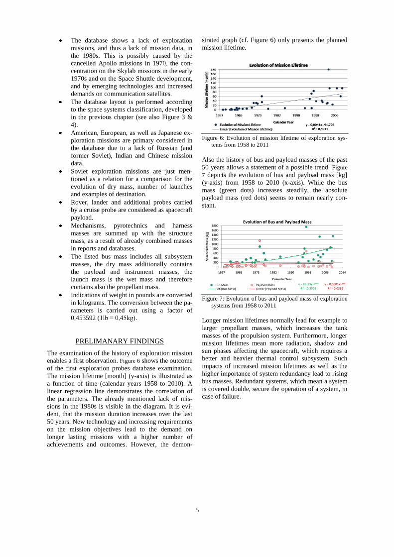
PRELIMANARY FINDINGS

The examination of the history of exploration mission

enables a first observation. Figure 6 shows the outcome

of the first exploration probes database examination.

The mission lifetime [month] (y-axis) is illustrated as

a function of time (calendar years 1958 to 2010). A

linear regression line demonstrates the correlation of

the parameters. The already mentioned lack of mis-

sions in the 1980s is visible in the diagram. It is evi-

dent, that the mission duration increases over the last

50 years. New technology and increasing requirements

on the mission objectives lead to the demand on

longer lasting missions with a higher number of

achievements and outcomes. However, the demon-

strated graph (cf. Figure 6) only presents the planned

mission lifetime.

Figure 6: Evolution of mission lifetime of exploration sys-

tems from 1958 to 2011

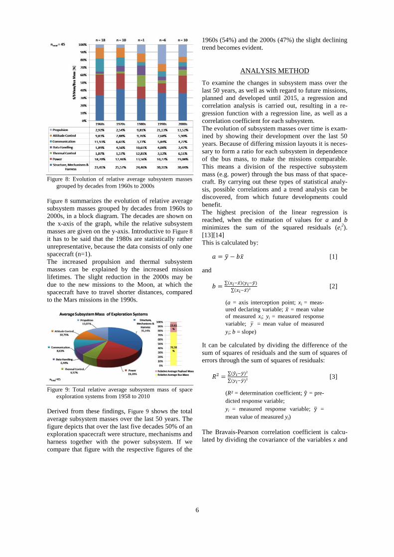
Also the history of bus and payload masses of the past

50 years allows a statement of a possible trend. Figure

7 depicts the evolution of bus and payload mass [kg]

(y-axis) from 1958 to 2010 (x-axis). While the bus

mass (green dots) increases steadily, the absolute

payload mass (red dots) seems to remain nearly con-

stant.

Figure 7: Evolution of bus and payload mass of exploration

systems from 1958 to 2011

Longer mission lifetimes normally lead for example to

larger propellant masses, which increases the tank

masses of the propulsion system. Furthermore, longer

mission lifetimes mean more radiation, shadow and

sun phases affecting the spacecraft, which requires a

better and heavier thermal control subsystem. Such

impacts of increased mission lifetimes as well as the

higher importance of system redundancy lead to rising

bus masses. Redundant systems, which mean a system

is covered double, secure the operation of a system, in

case of failure.

y = 8E-13x3,2606

R² = 0,3903y = 0,0001x1,2807

R² = 0,0336

0

200

400

600

800

1000

1200

1400

1600

1800

1957 1965 1973 1982 1990 1998 2006 2014

Spac

ecr

aft

Mas

s [k

g]

Calendar Year

Evolution of Bus and Payload Mass

Bus Mass Payload MassPot.(Bus Mass) Linear (Payload Mass)

6

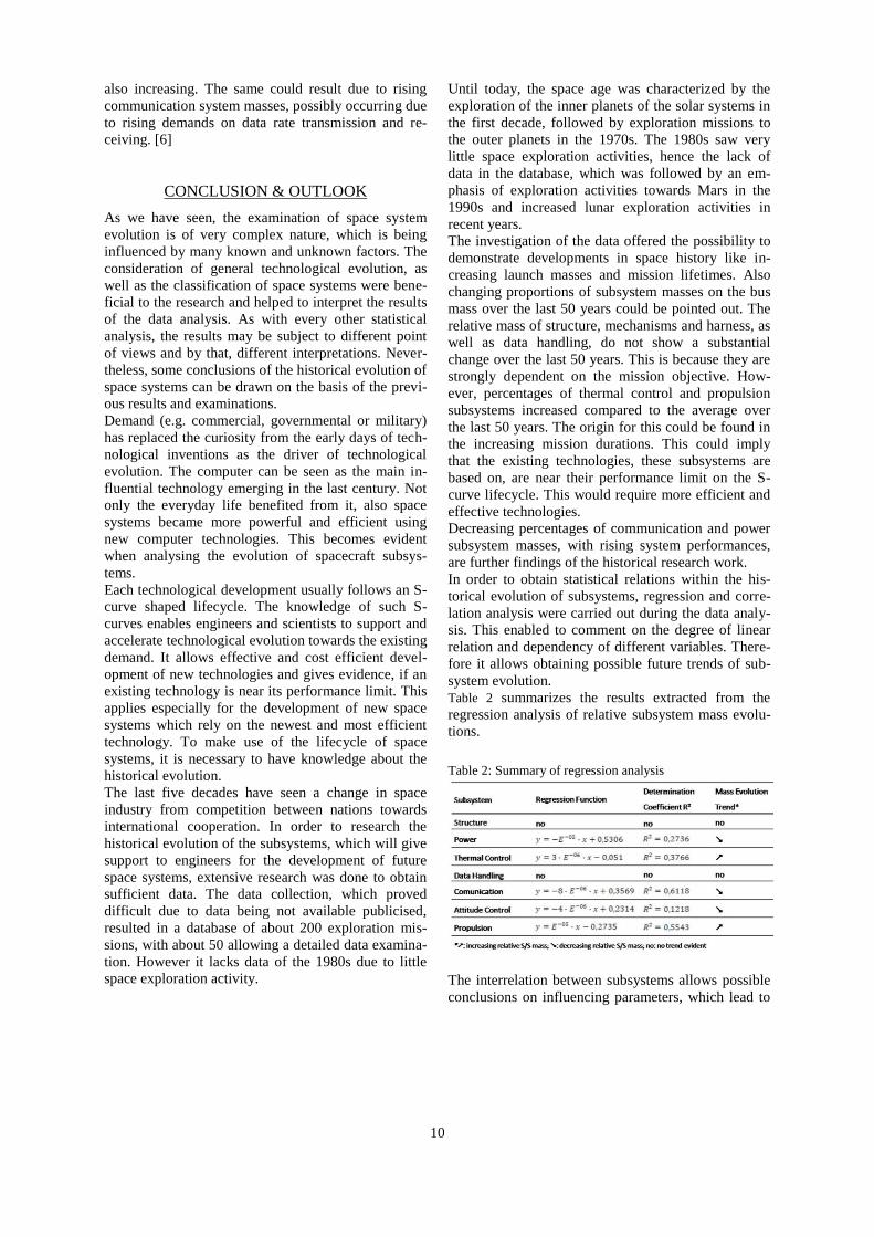
Figure 8: Evolution of relative average subsystem masses

grouped by decades from 1960s to 2000s

Figure 8 summarizes the evolution of relative average

subsystem masses grouped by decades from 1960s to

2000s, in a block diagram. The decades are shown on

the x-axis of the graph, while the relative subsystem

masses are given on the y-axis. Introductive to Figure 8

it has to be said that the 1980s are statistically rather

unrepresentative, because the data consists of only one

spacecraft (n=1).

The increased propulsion and thermal subsystem

masses can be explained by the increased mission

lifetimes. The slight reduction in the 2000s may be

due to the new missions to the Moon, at which the

spacecraft have to travel shorter distances, compared

to the Mars missions in the 1990s.

Figure 9: Total relative average subsystem mass of space

exploration systems from 1958 to 2010

Derived from these findings, Figure 9 shows the total

average subsystem masses over the last 50 years. The

figure depicts that over the last five decades 50% of an

exploration spacecraft were structure, mechanisms and

harness together with the power subsystem. If we

compare that figure with the respective figures of the

1960s (54%) and the 2000s (47%) the slight declining

trend becomes evident.

ANALYSIS METHOD

To examine the changes in subsystem mass over the

last 50 years, as well as with regard to future missions,

planned and developed until 2015, a regression and

correlation analysis is carried out, resulting in a re-

gression function with a regression line, as well as a

correlation coefficient for each subsystem.

The evolution of subsystem masses over time is exam-

ined by showing their development over the last 50

years. Because of differing mission layouts it is neces-

sary to form a ratio for each subsystem in dependence

of the bus mass, to make the missions comparable.

This means a division of the respective subsystem

mass (e.g. power) through the bus mass of that space-

craft. By carrying out these types of statistical analy-

sis, possible correlations and a trend analysis can be

discovered, from which future developments could

benefit.

The highest precision of the linear regression is

reached, when the estimation of values for a and b

minimizes the sum of the squared residuals (ei2).

[13][14]

This is calculated by:

[1]

and

[2]

(a = axis interception point; xi = meas-

ured declaring variable; = mean value

of measured xi; yi = measured response

variable; y = mean value of measured

yi; b = slope)

It can be calculated by dividing the difference of the

sum of squares of residuals and the sum of squares of

errors through the sum of squares of residuals:

[3]

(R² = determination coefficient; = pre-

dicted response variable;

yi = measured response variable; =

mean value of measured yi)

The Bravais-Pearson correlation coefficient is calcu-

lated by dividing the covariance of the variables x and

7

y through the standard deviations of the two variables

x and y.

[4]

(Cor = correlation coefficient; Cov(x,y)

= Coviariance of x and y; σ(x) = standard

deviation of x; σ(y) = standard deviation

of y)

The covariance (Cov) of two variables is the sum of

the product of the difference from the measured value

of the variables of their respective mean values:

[5]

(Cov(x;y) = Coviariance of x and y; n =

amount of measurements; xi = measured

declaring variable; = mean value of

measured xi;; yi = measured response

variable; y = mean value of measured yi)

The aim of this research work is to make a statement

about a possible trend in evolution of exploration

spacecraft systems. Although the gathered data repre-

sents just a quarter of all listed exploration missions

launched until today, it is possible to show an evolu-

tion trend of the last 50 years and possible trends of

subsystem mass growth. The figures of the following

chapter are based on 42 to 49 data points.

The number of data points does not allow a trend

analysis separate by mission destination, but it enables

the confirmation of a general evolution.

EVOLUTION OF EXPLORATION PROBE‟S

SUBSYSTEMS MASS

This chapter will visualize results of the data analysis

about the subsystem masses evolution of exploration

and deep space missions over the last 50 years. In

order to make the mission data comparable, a normali-

zation process has to be applied and the subsystem

masses are shown as a percentage of the bus mass of

the spacecraft. Thus, comparability between different

missions, with every spacecraft having a different bus

mass, is enabled. This chapter only shows a small

section of the full analysis. In order to see all mass

evolution charts, please refer to source [9].

Figure 10: Evolution of power subsystem mass of explora-

tion systems from 1958 to 2010

Figure 10 illustrates the power subsystem mass as a

proportion of the bus mass on the y-axis, in relation to

the time [calendar years], on the x-axis. The regres-

sion line is shown as well as the determination coeffi-

cient.

The last five decades show a slight decrease of relative

power subsystem masses although spacecrafts still

show a diverse proportion of power subsystem masses

of the overall mass. It is not easy to compare the

power subsystems with those of later, more sophisti-

cated probes. The reason for this is the first probes

being only equipped with primary batteries later also

small solar arrays as a source of power. More modern

probes however have large solar arrays and secondary

batteries, or even radioisotope thermoelectric genera-

tors (RTG), which are very differing technologies with

different system weights. The use of solar arrays is

also influenced by lightweight technologies, as they

have a high proportion of structure holding the solar

panels.

Figure 11: Evolution of Power Subsystem Performance of

exploration systems from 1958 to 2010

Figure 11 shows the evolution of the power subsystem

performance. It depicts the spacecraft‟s power output

[W] per kilogram mass (y-axis) over the calendar

years from 1958 to 2010 (x-axis). The data points of

17/02/1996 (NEAR Shoemaker mission to asteroid

Eros) and 24/10/1998 (Deep Space 1 mission to comet

y = -1E-05x + 0,5306R² = 0,2736

0%

10%

20%

30%

40%

50%

60%

70%

1957 1965 1973 1982 1990 1998 2006 2014Po

we

r S

/S m

ass/

Bu

s m

ass

[%]

Calendar Year

Evolution of Power Subsystem Mass

Evolution of Power System Mass

Linear (Evolution of Power System Mass)

8

Borrelly) with aberrant high values of 29,2W/kg and

24,07W/kg seem to present outlier. Looking at Figure

11 it is evident that there has been a slight increase in

the power output per kg of power subsystem mass.

This could be a reason for the decreasing power sub-

system mass, illustrated in Figure 10.

Figure 12: Evolution of data handling subsystem mass of

exploration systems from 1958 to 2010

Figure 12 shows the evolution of the data handling

subsystem masses. The mass of the data handling

subsystem as a proportion of the bus mass can be seen

on the y-axis, while the timeline in years is shown on

the x-axis.

Between the 1960s and 1970s the masses, as propor-

tion of the bus mass, of the data handling subsystem

seem to be split into two groups. One with rather low

data handling percentages of about 2% (Mariner and

Ranger missions), and another group with a percent-

age of about 10% (Pioneer). Today the mass propor-

tion is located between those two groups at 3% to 8%

of the overall bus mass.

There is no visible evolution noticeable. In average the

percentage of the data handling subsystem mass of the

overall mass seems to be rather constant.

Although there is no visible evolution in terms of an

increase or decrease of the proportion of the data han-

dling subsystem of the bus mass, that does not mean

that there have been no enhancements. They may well

have been qualitative enhancements, instead of quanti-

tative increase in mass, by the increase of the technol-

ogy efficiency.

Figure 13 depicts the evolution of the relative commu-

nication subsystem mass (y-axis) over the last 50

years (x-axis). A linear regression line, along with the

determination coefficient is also shown.

Figure 13: Evolution of communication subsystem mass of

exploration systems from 1958 to 2010

Besides the lack of exploration missions in the 1980s,

which can again be seen in this figure, two main clus-

ters of data points are visible. The first is beginning in

the end of the 1950s, lasting to the early 1970s, rang-

ing from a percentage of almost 25% to about 11%,

the second being situated between the mid 1990s and

today, ranging from about 8-9% down to about 1%. It

shows a clearly significant decrease of the communi-

cation subsystem proportion of the bus mass.

Accordingly, the communication technologies show,

that for example same bit rates require decreasing

output power; respectively rising bitrates are transmis-

sible with the same output power. Lower output power

need different amplifier, like with semiconductor

technologies, which enable lighter components.

Changes in wave band (spectrum), e.g. from S-band to

X- and Ka-band, mean smaller wave length, and con-

sequently smaller components like antennas.

But also the evolution of electronic devices allowed

producing smaller components, which are lighter and

provide a higher performance at the same time. The

development from normal soldering joints to surface-

mounting technology (SMT) with so called surface

mounted devices (SMD), lead to weight savings due

to the electrotechnology development itself. All listed

factors may have influenced the decrease of commu-

nication subsystem masses towards smaller propor-

tions of the bus mass.

INTERRELATION OF SUBSYSTEMS MASS

BEHAVIOR

The evolution of the subsystem masses are affected by

a diversity of unknown parameters. Some parameters

can only be assumed. To understand the influences,

which affect the subsystem‟s masses, interrelations

between subsystems are examined in this chapter. A

subsystem‟s reaction or influence on another subsys-

tem‟s mass change, can give an idea on possible de-

9

pendencies. Consequently, a possible influence pa-

rameter on the evolution could be identified.

From the high diversity of possible subsystem varie-

ties, only the significant ones are presented, showing

at least a correlation coefficient higher or equal than

0,3 for a positive correlation, or lower or equal than -

0,3 for a negative correlation. According to some

authors, such a coefficient means at least a correlation

of medium strength between the two examined sub-

system mass behaviours. [15][16]

Figure 14 describes the relative AOCS mass as a func-

tion of the relative communication subsystem mass.

The relative AOCS mass is plotted on the y-axis and

the relative communication subsystem mass on the x-

axis. A linear regression line with y=0,7585x+0,0115

shows the relation of the subsystem masses with a

determination coefficient of R²=0,38 and a correlation

coefficient of about Cor=0,61. Most of the data points

show the relative AOCS masses between 1% and 8%

being linked to the respective relative communication

masses between 1% and 10%.

Figure 14: Correlation of attitude and orbital control S/S and

communication S/S of exploration systems (1958 to

2010)

The correlation coefficient of Cor=0,61 shows a rather

strong linear relation between the two variables. The

determination coefficient of R²=0,38 furthermore

explains a medium strong dependency of the relative

AOCS mass on the relative communication mass. This

could mean if the relative mass of the communication

system is increasing, the relative AOCS mass has also

to be increased.

Longer spacecraft antennas or bigger parabolic anten-

nas allow a better and greater data transmission and

reception. To achieve that, the transmission beam has

to be more focused and narrow. In order to keep the

direction focused within the narrow limitations of the

beam, the AOCS has to be better dimensioned with a

better performance, and thus will be heavier.

Figure 15 describes the relative power subsystem mass

(y-axis) as a function of the relative data handling

subsystem mass (x-axis), and Figure 16 as a function of

the relative communication subsystem mass (x-axis).

Both relations are shown with a linear regression line.

A cluster of relative data handling subsystem masses

can be seen in Figure 15 between 1% and 4% with a

relative power subsystem mass between 1% and 30%.

A little less compact cluster between 6% and 10% of

relative data handling subsystem mass with a relative

power subsystem mass between 10% and 50%, can be

seen in Figure 16.

Figure 15: Correlation of power S/S mass and data handling

S/S mass of exploration systems (1958 to 2010)

Both figures have similar correlation coefficients of

Cor=0,39 and Cor=0,37, which respectively means in

both cases a linear relation of medium strength be-

tween the respective relative subsystem masses.

The determination coefficients in both figures are

rather weak with values of R²=0,15 and R²=0,14. So,

there is only a slight dependence of the power subsys-

tem mass towards the data handling and communica-

tion subsystem mass.

The dependency of the relative power subsystem mass

towards the relative data handling mass and relative

communication mass could be the increased power

consumption of increasing data handling and commu-

nication systems. [6]

Figure 16: Correlation of power S/S mass and communica-

tion S/S mass of exploration systems (1958 to 2010)

If the relative data handling subsystem mass, perhaps

due to rising thermal control requirements, increases,

it could result in the relative power subsystem mass

10

also increasing. The same could result due to rising

communication system masses, possibly occurring due

to rising demands on data rate transmission and re-

ceiving. [6]

CONCLUSION & OUTLOOK

As we have seen, the examination of space system

evolution is of very complex nature, which is being

influenced by many known and unknown factors. The

consideration of general technological evolution, as

well as the classification of space systems were bene-

ficial to the research and helped to interpret the results

of the data analysis. As with every other statistical

analysis, the results may be subject to different point

of views and by that, different interpretations. Never-

theless, some conclusions of the historical evolution of

space systems can be drawn on the basis of the previ-

ous results and examinations.

Demand (e.g. commercial, governmental or military)

has replaced the curiosity from the early days of tech-

nological inventions as the driver of technological

evolution. The computer can be seen as the main in-

fluential technology emerging in the last century. Not

only the everyday life benefited from it, also space

systems became more powerful and efficient using

new computer technologies. This becomes evident

when analysing the evolution of spacecraft subsys-

tems.

Each technological development usually follows an S-

curve shaped lifecycle. The knowledge of such S-

curves enables engineers and scientists to support and

accelerate technological evolution towards the existing

demand. It allows effective and cost efficient devel-

opment of new technologies and gives evidence, if an

existing technology is near its performance limit. This

applies especially for the development of new space

systems which rely on the newest and most efficient

technology. To make use of the lifecycle of space

systems, it is necessary to have knowledge about the

historical evolution.

The last five decades have seen a change in space

industry from competition between nations towards

international cooperation. In order to research the

historical evolution of the subsystems, which will give

support to engineers for the development of future

space systems, extensive research was done to obtain

sufficient data. The data collection, which proved

difficult due to data being not available publicised,

resulted in a database of about 200 exploration mis-

sions, with about 50 allowing a detailed data examina-

tion. However it lacks data of the 1980s due to little

space exploration activity.

Until today, the space age was characterized by the

exploration of the inner planets of the solar systems in

the first decade, followed by exploration missions to

the outer planets in the 1970s. The 1980s saw very

little space exploration activities, hence the lack of

data in the database, which was followed by an em-

phasis of exploration activities towards Mars in the

1990s and increased lunar exploration activities in

recent years.

The investigation of the data offered the possibility to

demonstrate developments in space history like in-

creasing launch masses and mission lifetimes. Also

changing proportions of subsystem masses on the bus

mass over the last 50 years could be pointed out. The

relative mass of structure, mechanisms and harness, as

well as data handling, do not show a substantial

change over the last 50 years. This is because they are

strongly dependent on the mission objective. How-

ever, percentages of thermal control and propulsion

subsystems increased compared to the average over

the last 50 years. The origin for this could be found in

the increasing mission durations. This could imply

that the existing technologies, these subsystems are

based on, are near their performance limit on the S-

curve lifecycle. This would require more efficient and

effective technologies.

Decreasing percentages of communication and power

subsystem masses, with rising system performances,

are further findings of the historical research work.

In order to obtain statistical relations within the his-

torical evolution of subsystems, regression and corre-

lation analysis were carried out during the data analy-

sis. This enabled to comment on the degree of linear

relation and dependency of different variables. There-

fore it allows obtaining possible future trends of sub-

system evolution.

Table 2 summarizes the results extracted from the

regression analysis of relative subsystem mass evolu-

tions.

Table 2: Summary of regression analysis

The interrelation between subsystems allows possible

conclusions on influencing parameters, which lead to

11

changes in the proportion of subsystem masses over

the last 50 years of space exploration.

Strong correlations between mass proportion changes

in the attitude and orbital control subsystem (AOCS)

and the structure, as well as the communication sub-

system were pointed out. Furthermore, interrelations

between mass proportion changes between data han-

dling and thermal control subsystems, as well as be-

tween the power and data handling subsystems, as

well as between the power and communication sub-

systems, were demonstrated.

Table 3 summarizes the results extracted from the

correlation analysis of subsystem mass change rela-

tions.

Additionally, the assumption, that increasing bus

masses lead to increasing subsystem masses, inde-

pendently from the payload mass, has been confirmed.

Increasing subsystem masses showed a strong correla-

tion (Cor=0,55 to 0,85) to increasing bus masses, just

with little less characteristic in the thermal control and

communication subsystem, as well as in the attitude

and orbital control subsystem.

Table 3: Summary of correlation factors between different

subsystems (S/S)

Based on the development of the past 50 years, it can

be assumed that relative subsystem masses of subsys-

tems like power or communication will decrease fur-

ther. This will be possible on the basis of the future

evolution of technical systems providing a higher

performance level with lower requirements towards

size and mass, hence a higher degree of efficiency.

Propulsion and thermal control subsystems are likely

to increase in relative mass if no new and more effi-

cient technologies are introduced. This assumption is

based on the tendency of space missions having grow-

ing mission durations with several mission objectives,

which require these subsystems to provide higher

performance.

Because of the fundamental role of the structure,

mechanisms and harness, the relative mass of this

subsystem is not likely to change significantly. Never-

theless minor changes could be possible by using new

lightweight structures such as composites for building

the spacecraft structure. The attitude and orbital con-

trol subsystem have not seen significant changes in

relative mass over the past 20 years, which seems to

be a trend for future AOCSs.

The shown interrelations between subsystems will

help to support future Concurrent Engineering studies

at the Concurrent Engineering Facility (CEF) within

the Institute for Space Systems (DLR), Germany.

Subsystem mass trends and interrelationships between

different subsystems will help the engineers to evalu-

ate their calculation and estimates.

Future investigations will concentrate on Earth orbit-

ing satellites and spacecrafts, where a bigger base of

primary data is anticipated.

ACKNOWLEDGEMENT

The paper was prepared within the Department of

System Analysis Space Segment at the Institute of

Space Systems (German Aerospace Center – DLR)

Bremen, in cooperation with the University of Applied

Sciences Bremen, Germany.

REFERENCES

[1] Darwin, Charles: The Origin of Species. Edited

with an introduction and notes by Gillian Beer, Ox-

ford University Press, 1998.

[2] Darwin, Charles, Neumann, Carl W.: Die Entste-

hung der Arten. Nikol Verlag, 2004.

[3] Hill, Bernd: Gesetzmäßigkeiten der Technikevolu-

tion: Mittel zur Ausprägung von technischem Ent-

wicklungsverständnis und technischer Gestaltungsfä-

higkeit. In: Technica Didactica, 4. Edition 2000/Bd.1,

Hildesheim: Franzbecker Verlag, 2000, pp. 3-26.

[4] Altschuller, G. S.: Erfinden: Wege zur Lösung

technischer Probleme. Berlin: Verlag Technik, 1984.

[5] Gemünden, Hans G.: Management of Innovation I:

Technology and Innovation Management. Berlin:

Technical University, 2005, p.25.

[6] Dessauer, F.: Streit um die Technik. 2nd Edition,

Frankfurt, 1958.

[7] Adner, Ron; Levinthal, Daniel: Demand Heteroge-

neity and Technology Evolution: Implications for

12

Product and Process Innovation. In: Management

Science Vol. 47, No.5, May 2001, pp.611-628.

[8] Wölfel, Silvia: Evolution von Technik: Gerichte-

theit von Technikentwicklung?. Seminararbeit, Dres-

den: Technical University, 2004.

[9] Stellmann, Svenja: Historical Technology Evolu-

tion of Space Systems: with Special Regards towards

Subsystems. Bremen: University of Applied Sciences

Bremen, German Aerospace Center (DLR), Germany,

2009.

[10] NSSDC Master Catalog Search. National Aero-

nautics and Space Administration 2008.

http://nssdc.gsfc.nasa.gov/nmc/SpacecraftQuery.jsp,

Retrieved: 01/03/2009

[11] Wade, Mark: Encyclopedia Astronautica. 2008.

http://www.astronautix.com, Retrieved: 04/03/2009

[12] Union of Concerned Scientists: Satellite Data-

base. UCS Database, 2009.

http://www.ucsusa.org, Retrieved: 03/03/2009

[13] Kohn, Wolfgang: Statistik: Datenanalysis und

Wahrscheinlichkeits-rechnung. Berlin: Springer-

Verlag, 2005.

[14] Toutenburg, Helge; Heumann, Christian: Desk-

riptive Statistik: Eine Einführung in Methoden und

Anwendungen mit R und SPSS. Berlin: Springer-

Verlag, 2008.

[15] Schmidt, Peter: Statistik in 25 Schritten. Edition

4.1, Bremen: University of Applied Sciences, 2007.

[16] Wikipedia: Correlation. The Free Encyclopedia,

2009.

http://en.wikipedia.org/wiki/Correlation, Retrieved:

30/03/09