Historical controls in clinical trials: the meta-analytic - Bayes-pharma

Historical controls in clinical trials: themeta-analytic predictive approach applied

to over-dispersed count data

Sandro Gsteiger, Beat Neuenschwander, and HeinzSchmidli

Novartis Pharma AG

Bayes Pharma, Aachen, May 2012

Table of contents

Introduction

Methodology (MAP)

Applications

Conclusions

1

Table of contents

Introduction

Methodology (MAP)

Applications

Conclusions

2

Introduction

• Relevant information always available

• Informal use in trial design and planning is standard– Endpoints– Design options– Assumptions for sample size calculation

• Increasing interest in formal use also for analysis– Methodological: bias model, power priors, meta-analytic

predictive priors (hierarchical modeling), commensuratepriors. Approaches similar in spirit; closely relatedformalisms.

– Practical (orphan indications, medical devices, pediatrics)

• Key issue: proper discounting of historical data– How much do we know?– ”Worth” how many patients, n∗?

3

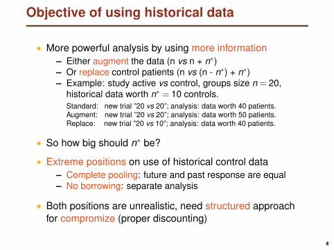
Objective of using historical data

• More powerful analysis by using more information– Either augment the data (n vs n + n∗)– Or replace control patients (n vs (n - n∗) + n∗)– Example: study active vs control, groups size n = 20,

historical data worth n∗ = 10 controls.Standard: new trial ”20 vs 20”; analysis: data worth 40 patients.Augment: new trial ”20 vs 20”; analysis: data worth 50 patients.Replace: new trial ”20 vs 10”; analysis: data worth 40 patients.

• So how big should n∗ be?

• Extreme positions on use of historical control data– Complete pooling: future and past response are equal– No borrowing: separate analysis

• Both positions are unrealistic, need structured approachfor compromize (proper discounting)

4

Design issues

Trying to predicting the future from knowing the past

• Difficult problem!• In indication ABC, placebo

response is about ...• How well do we know the past,

how much can we predict?

• Sometimes prediction withconfidence...

• ... or with large uncertainty.

●

●

●

●

●

Historical data

New ?

5

Analysis issues

• Analysis: fundamentally, two philosophies1. Joint analysis of historical and new data at end of new

study (with parameter of interest effect in new trial)2. Derive informative prior upfront

• Mathematically both approaches equivalent (in principle)

• Will focus on construction of historical data prior– Conceptually clear separation of information sources– Quantification of information upfront (n∗)

• Challenges for communication with clinical teams– Two sources of information– Possibility of conflict

6

Extension to MAP approach studied here

• MAP was introduced for (approx.) normal endpoints

• Objective here: apply to over-dispersed counts– Consider two data sources: summary and individual level– Summary level: literature, trial repositories etc.– Individual level: in-house trials

• Examples of over-dispersed counts in pharma– Multiple sclerosis: lesion counts on MRI scans, number of

relapses– COPD: number of exacerbations– Number of AEs within a patient– ...

7

Table of contents

Introduction

Methodology (MAP)

Applications

Conclusions

8

The meta-analytic predictive approach

Historical trials, h = 1, ...,H:

yh ∼ F (θh ; nh, ...)

New trial: Y ∗ ∼ F (θ ∗ ; ...)

Exchangeability assumption:

θ1, ...,θH ,θ ∗|η ,τiid∼ N(η ,τ2)

Prior for new trial mean:π(θ ∗|y1, ...,yH)

”Worth” n∗ patients(prior effective sample size).

●

●

●

●

●

Historical data

Posterior of η

Predictive distributionfor θ*

n* large (close to N)

n* very small

9

Exchangeability - the key assumption

• Formally: π(θ1, . . . ,θH ,θ ∗) is permutation invariant– Difficult to communicate to clinical teams– ”For any two randomly selected trials, no specific ordering

between underlying means expected.”

• May apply after covariate adjustment (meta-regression).

• In practice, not always considered carefully enough– The new trial mean θ ∗ is part of it– Changes in trial design may lead to new round of MAP (e.g.

inclusion criteria)– Trial design: iterative process; MA: time-consuming

• Potential source of prior-data conflict if violated

10

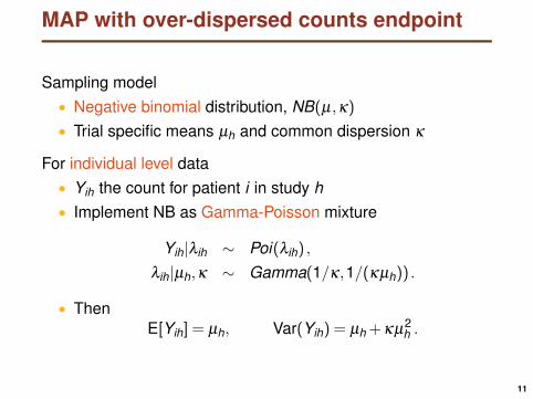
MAP with over-dispersed counts endpoint

Sampling model• Negative binomial distribution, NB(µ,κ)

• Trial specific means µh and common dispersion κ

For individual level data• Yih the count for patient i in study h• Implement NB as Gamma-Poisson mixture

Yih|λih ∼ Poi(λih) ,

λih|µh,κ ∼ Gamma(1/κ,1/(κµh)) .

• ThenE[Yih] = µh, Var(Yih) = µh +κµ

2h .

11

MAP with over-dispersed counts (ctd)

Summary level data• Only observed means µ̂h = ∑i Yih/nh given• This sum of NBs is again NB,

∑i

Yih ∼ NB(nhµh,κ/nh)

Exchangeable log-means, θh = log(µh) ,

θ1, . . . ,θH ,θ ∗|η ,τ ∼ N(η ,τ2) .

12

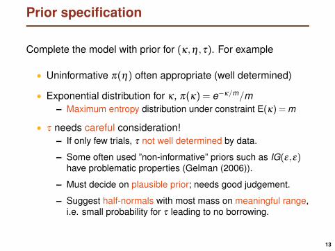
Prior specification

Complete the model with prior for (κ,η ,τ). For example

• Uninformative π(η) often appropriate (well determined)

• Exponential distribution for κ, π(κ) = e−κ/m/m– Maximum entropy distribution under constraint E(κ) = m

• τ needs careful consideration!– If only few trials, τ not well determined by data.

– Some often used ”non-informative” priors such as IG(ε,ε)have problematic properties (Gelman (2006)).

– Must decide on plausible prior; needs good judgement.

– Suggest half-normals with most mass on meaningful range,i.e. small probability for τ leading to no borrowing.

13

Prior effective sample size

Analysis of new trial using the historical data: take posteriorpredictive distribution π(θ ∗|y) as prior for placebo group in newstudy.

If π(θ ∗|y) approximate normal, prior effective sample size(Neuenschwander et al. (2010))

n∗ = NVar(θ ∗|y ,τ = 0)

Var(θ ∗|y).

• Ballpark figure; tool for design of new study.• O.k. in the NB example later on., but other cases may need

different approximations; e.g. if Beta(a,b), then n∗ = a+b.

14

Table of contents

Introduction

Methodology (MAP)

Applications

Conclusions

15

Example: lesion counts in multiple sclerosis

• Progressive, degenerative diseaseof the central nervous system

• Inflammation and tissue damage inthe brain

• Lesions on MRI scans used indiagnosis and monitoring of diseaseevolution

• Lesions serve as (early) markers inclinical trials

• Lesion counts typicallyover-dispersed

16

Data overview (placebo patients)

Baseline enrichment• Enrol only patients with ≥ 1 lesion at baseline• Minimal disease activity (more homogeneous population)

A BStudy nh µ̂h nh µ̂h

In-house Kappos2006 81 2.2 41 3.29Kappos2010 373 1.32 129 2.91Saida2012 50 1.38 20 2.8

Literature Myhr1999 32 1.6Filippi2006 548 1.73Polman2006 315 1.3Hauser2008 35 1.375Kappos2008 65 1.125Giovannoni2010 437 0.91Comi2001 120 3.5Comi2008 102 3.9

GdE T1 lesions at 6 months; without (A) and with B baseline enrichment.17

Application 1: no baseline enrichment

• 3 in-house (individual level data), 6 literature trials

• N=1936 historical patients (504 in-house, 1432 literature)

• Approach for prior τ

– Use half-normal• Ensures positive mass around small heterogeneity• Weight in reasonnable range (not ”heavy tailed”)

– Need to compare within- (σ ) and between-trial variability (τ)

– Very large heterogeneity: ”τ ≈ σ = SD(logY )”

– σ̂ ≈ 2 from in-house data

– Set median(π(τ)) = σ̂ (i.e. HN(scale=3))

– Alternative: HN(scale=1), centered between substantialand large heterogeneity (Spiegelhalter et al. (2004))

18

Application 1: results

Study mean

●●Saida2012

●●Kappos2006

●●Kappos2010

●●Myhr1999

●●Filippi2006

●●Polman2006

●●Hauser2008

●●Kappos2008

●●Giovannoni2010

●●New

A

0.5 1.0 1.5 2.0 2.5 3.0 3.5

Prior n∗

HN(scale=3) 25HN(scale=1) 29

Heterogeneity τ (fixed) n∗

small 0.125 148moderate 0.25 40substantial 0.5 11large 1 3very large 2 1

Data indicate moderate to

substantial heterogeneity.

19

Application 2: use baseline enrichment

• Enrol patients with ≥ 1 lesion at baseline

• Minimal disease activity; homogeneity of study population

• Different trial than in application 1!

• 3 in-house (individual level data), 2 literature trials

• N=412 (190 in-house, 222 literature)

• Approach for prior τ ∼ HN(ν2)

– Small number of trials, need informative prior– Less heterogeneity expected than in application 1– Set ν such that 90% quantile of prior is equal to 90%

quantile of posterior for τ from application 1.

20

Priors and posteriors for τ

τ

Den

sity

0.0 0.2 0.4 0.6 0.8 1.0

01

23

45 A

τ

Den

sity

0.0 0.2 0.4 0.6 0.8 1.0

01

23

45

6 B

21

Application 2: results

Study mean

●●Saida2012

●●Kappos2006

●●Kappos2010

●●Comi2001

●●Comi2008

●●New

2.0 2.5 3.0 3.5 4.0 4.5 5.0 5.5

Prior n∗

HN(scale=0.26) 62

Heterogeneity τ (fixed) n∗

small 0.125 75moderate 0.25 23substantial 0.5 6large 1 1very large 2 0

Data indicate small to moderate

heterogeneity.

22

Table of contents

Introduction

Methodology (MAP)

Applications

Conclusions

23

Conclusions

• Historical data included in the analysis can lead to quickerand more ethical trials

– Less patients on placebo– Potentially faster recruitement

• The actual number of patients to be replaced in new trialdepends on various factors, not just n∗

– Randomization– Objectives of trial; secondary and exploratory endpoints– Confidence of team with approach

• Analysis of new trial more difficult– Not for the Bayesian (”it’s just using a certain prior”)– ... but for the clinical team yes (not used to statistical

analysis with different sources of information).

24

References

Spiegelhalter DJ, Abrams KR, Myles JP. (2004) Bayesian Approaches to Clinical Trials and Health-CareEvaluation. Wiley.Berry et al. (2010) Bayesian Adaptive Methods for Clinical Trials. Chapman & Hall.Pocock S. (1976) The combination of randomized and historical controls in clinical trials. Journal of ChronicDiseases.brahim and Chen (2000) Power prior distributions for regression models. Statistical Science 15:46-60.Neuenschwander B, Capkun-Niggli G, Branson M, Spiegelhalter DJ. Summarizing historical information oncontrols in clinical trials, Clinical Trials. 2010.Hobbs et al. (2011) Hierarchical Commensurate and Power Prior Models for Adaptive Incorporation of HistoricalInformation in Clinical Trials. Biometrics.Sormani et al. Modelling MRI enhancing lesion counts in multiple sclerosis using a negative binomial model:implications for clinical trials. J Neurol Sci. 1999.

25

Review of methods

See reviews in Spiegelhalter et al (2004), Berry et al (2010).• Bias model (Pocock (1976)), θh = θ +δh

• Power priors (Ibrahim& Chen (2000)),

π(θ |D0,α) ∝ L(θ |D0)α

π0(θ), 0≤ α ≤ 1

• Commensurate priors (Hobbs et al. (2011))– Explicitly parameterize similarity between D and D0– Commensurability parameter τ

– π(θ |D0,θ0,τ) ∝ ...π(θ |θ0,τ)...

• Random effects meta-analytic predictive (MAP) appraoch(Spiegelhalter et al (2004), Neuenschwander et al. (2010))

26

Structure of WinBUGS code

model{

## data generating model

for(i in 1:ntot){ # exchangeable std log-means

theta[i] ~ dnorm(eta, inv.tau2)

...

}

for(i in 1:nobs){ # likelihood: in-house data

...

lambda[i] ~ dgamma(k.inv, kmu.inv[i])I(0.001,) # for num stability

y[i] ~ dpois(lambda[i])

}

for(i in 1:nlit){ # likelihood: literature data

...

xm[i] ~ dgamma(alpha[i], beta[i])I(0.001,)

ym[i] ~ dpois(xm[i])

}

## new study mean and new obs

theta.new ~ dnorm(eta, inv.tau2)

mu.new <- exp(theta.new)

...

## priors

inv.tau2 <- 1/(tau*tau)

tau ~ dnorm(0, pprec.tau)I(0,)

...

}

27

Historical controls in clinical trials: the meta-analytic - Bayes-pharma

Documents

Transcript of Historical controls in clinical trials: the meta-analytic - Bayes-pharma