Highly Adaptive Liquid Simulations on Tetrahedral Meshes

Ryoichi Ando∗

Kyushu UniversityNils Thurey†

ScanlineVFXChris Wojtan‡

IST Austria

Figure 1: Our adaptive simulation framework allows us to efficiently simulate highly detailed splashes on large open surfaces. In this case,maximum BCC mesh resolutions from 8 to 1024 cells were used, leading to strong horizontal grading along the surface.

Abstract

We introduce a new method for efficiently simulating liquid withextreme amounts of spatial adaptivity. Our method combines sev-eral key components to drastically speed up the simulation of large-scale fluid phenomena: We leverage an alternative Eulerian tetra-hedral mesh discretization to significantly reduce the complexity ofthe pressure solve while increasing the robustness with respect to el-ement quality and removing the possibility of locking. Next, we en-able subtle free-surface phenomena by deriving novel second-orderboundary conditions consistent with our discretization. We cou-ple this discretization with a spatially adaptive Fluid-Implicit Parti-cle (FLIP) method, enabling efficient, robust, minimally-dissipativesimulations that can undergo sharp changes in spatial resolutionwhile minimizing artifacts. Along the way, we provide a newmethod for generating a smooth and detailed surface from a set ofparticles with variable sizes. Finally, we explore several new sizingfunctions for determining spatially adaptive simulation resolutions,and we show how to couple them to our simulator. We combineeach of these elements to produce a simulation algorithm that iscapable of creating animations at high maximum resolutions whileavoiding common pitfalls like inaccurate boundary conditions andinefficient computation.

CR Categories: I.3.7 [Computer Graphics]: Three-DimensionalGraphics and Realism—Animation; I.3.5 [Computer Graphics]:Computational Geometry and Object Modeling—Physically basedmodeling

Keywords: fluid simulation, tetrahedral discretization, adaptivity

∗E-mail:and@verygood.aid.design.kyushu-u.ac.jp†E-mail:nils.thuerey@scanlinevfx.com‡E-mail:wojtan@ist.ac.at

Links: DL PDF

1 Introduction

This paper aims to produce fluid simulations with a high degree ofspatial adaptivity. We desire to enable a simulator to focus its com-putational resources on the visually interesting regions of a fluidflow, while remaining computationally efficient and avoiding com-mon artifacts due to a spatially adaptive pressure solve.

Previous approaches have made great strides towards this goal, butthey often exhibit visual artifacts, a lack of computational robust-ness, or an unacceptably hefty computational expense. The ground-breaking work of Losasso et al. [2004] introduced an octree forspatial adaptivity, but it suffers from spurious flows at T-junctions.Finite volume methods [Batty et al. 2010] repair these spatial arti-facts at the expense of solving a significantly larger system of equa-tions and sacrificing computational stability near poorly-shaped el-ements. Furthermore, many existing methods still are not truly spa-tially adaptive in the sense that their computational complexity isstill tied to a uniform grid or spatial parameter.

We introduce a combination of techniques that successfully makes

adaptive fluid simulation practical at large scales. We first reducememory and computational costs by switching from a finite volumemethod to a discretization with a significantly smaller linear sys-tem for the pressure solve, which has the side effect of increasingthe simulator’s robustness to poor-quality elements and effectivelypreventing locking artifacts. We next derive second-order Dirich-let boundary conditions consistent with our discretization to benefitfrom the subtle surface dynamics associated with an accurate pres-sure solve. We combine this robust and efficient tetrahedral mesh-based fluid simulator with a spatially adaptive method for samplingparticles for FLIP-based velocity advection, giving us a method freefrom any single spatial resolution.

In addition to our adaptive FLIP simulator, we also introduce a newmethod for computing a surface from a distribution of particleswith variable radii. We found that this method out-performs pre-vious methods in cases of extreme spatial adaptivity by exhibitingsmoother surfaces without sacrificing detail.

Our fluid simulator works well with spatially adaptive tetrahedralmeshes, but it is another question to decide exactly how these adap-tive meshes should be generated. We investigate various methodsfor generating these adaptive meshes by experimenting with severalsizing functions, allowing us to precisely dictate where simulationdetail should occur. Some examples are a surface curvature-basedmetric that adds detail only where needed on the fluid surface, aturbulence metric that adds detail only where interesting fluid mo-tion occurs, and a visibility metric that adds detail only in front ofa virtual camera.

Concretely, the contributions of our work are:• a novel tetrahedral discretization of the pressure projection

step that is efficient to solve and robust to poor-quality ele-ments;

• an accurate treatment of second-order boundary conditionswithin the tetrahedral mesh;

• a new technique for extracting a smooth surface from particleswith varying radii;

• and the inclusion of a flexible sizing function to focus compu-tational resources on important areas of the flow with minimaloverhead.

These contributions work together to produce a practical fluid sim-ulator that exhibits low computational and memory complexity,fewer visual artifacts, and a high effective simulation resolution.

2 Related Work

Our work is based on the Fluid-Implicit Particle (FLIP) methodintroduced to the computer graphics community by Zhu and Brid-son [2005], which arguably represents the state-of the art for de-tailed and robust liquid simulations. The algorithm still followsthe general ideas of the Stable Fluid solver [Stam 1999], and canbe readily combined with second-order treatment of free surfaceboundary conditions [Enright et al. 2003]. FLIP derives its successfrom the fact that it uses particles to compute an accurate, non-diffusive transport of flow quantities, in combination with a grid-based solve to accurately enforce constraints for mass conservation.The FLIP algorithm is heavily used in the special effects industry,and recent advances have introduced accurate coupling with obsta-cles [Batty et al. 2007], highly viscous materials [Batty and Bridson2008], and two-phase flows [Boyd and Bridson 2012].

Traditionally, Cartesian grids are very popular for fluid simulations.The Marker-And-Cell (MAC) approach [Harlow and Welch 1965],which stores velocity components at cell faces and pressure sam-ples at cell centers, results in discretizations with good properties in

terms of stability and accuracy. An inherent difficulty is that sim-ulations on regular grids become prohibitively expensive for largeresolutions. Thus, many works have proposed methods to focus thecomputations on regions that are of particular interest. One exam-ple are octrees, which were used by Losasso et al. [2004; 2005] torefine the computational grid in a controllable way. This approach,however, suffers from numerical diffusion and an inconsistent dis-cretization near the tree’s T-junctions. Targeting a similar direc-tion as our work, Hong et al. [2009] and Ando et al. [2012] havedemonstrated methods to adapt the resolution of FLIP particles in asimulation. Both methods, in contrast to ours, focus on static com-putational grids and are restricted to smaller differences in particlesize.

Although Cartesian grids are widely used, they are limited in theirflexibility to adapt to a simulation setup. Because of this, tetrahe-dral grids are popular for methods targeting adaptivity. In combina-tion with a suitable method to discretize the problem at hand, theyallow for very flexible computational grids. One example is thework of Klingner et al. [Klingner et al. 2006] which demonstratedthe use of a Stable Fluids based solver for tetrahedral grids con-forming to object boundaries. Another example is the non-linearfluid solver developed by Mullen et al. [2009], which leads to anenergy conserving solve. Unlike these methods, we make use ofa non-conforming grid with Body-Centered Cubic (BCC) lattices.These meshes were also used by Chentanez et al. [2007] and byBatty et al. [2010] for liquid simulations. We will denote this classof algorithms as Finite Volume Methods (FVM). These methodsare primarily suitable for uniformly sampled particles, and we willdemonstrate in Section 7 that their placement of pressure samplesat tetrahedral circumcenters leads to numerical problems in combi-nation with graded BCC meshes.

Another direction of research performs fluid simulations based onarbitrary elements. Clausen et al. [2013] and Misztal et al. [2010]have proposed a method to simulate liquids with a computationalgrid conforming to a triangulation of a liquid surface. Both meth-ods lead to an increased computational cost in comparison to themore efficient tetrahedral BCC meshes. Sin et al. [2009] pro-posed an alternative method for hybrid Lagrangian-Eulerian solverswhich combines a Voronoi-based pressure solver and particles. Us-ing this Vornoi-based approach for tetrahedral meshes would yielda pressure matrix similar to ours. Like our method, Brochu etal. [2010] used this discretization in combination with embeddedsecond-order boundary conditions. Both of these approaches dis-cretize velocities with per-face flux values, while we store velocityvectors at cell barycenters.

Adaptive simulations have also been explored in the context of SPHsimulations without Eulerian grids. The work of [Adams et al.2007] shares similarities with our approach, as it is able to simulatea wider range of particle radii, and it proposes a surface reconstruc-tion method in the adaptive setting. We will show in Section 5 thatour surface creation method results in surfaces with fewer visualartifacts. Additionally, a robust and efficient method for adaptiveSPH simulations was introduced by Solenthaler et al. [2011], butthis work primarily targets the coupling of two different particleresolutions.

Several other methods have been proposed to reconstruct smoothsurfaces around collections of particles without orientation. Oneapproach that is commonly used is to compute a signed distancefunction with averaged particle radii and centroids [Zhu and Brid-son 2005]. A variant of this approach, taking into account informa-tion about the spatial variance of the particle’s neighborhood wasproposed by Yu et al. [2010]. Both methods primarily target parti-cles with constant radius. More recently, a level-set based methodwas proposed that computes a constrained optimization with bihar-

monic smoothing [Bhattacharya et al. 2011]. However, such an op-timization would be complicated to apply in our unstructured set-ting. In contrast to these methods, our approach for surface cre-ation computes the union of convex hulls around triplets of parti-cles, which leads to a smooth and closed surface around a collectionof arbitrarily sized particles.

3 Fluid Solver

The aim of our method is to solve the Navier-Stokes equations,which for incompressible, Newtonian, inviscid flows can be writtenas ρDu/Dt = −∇p+ f , with the additional constraint∇ · u = 0to enforce a divergence-free velocity field. Here, u, p and f denotevelocity, pressure and external forces, respectively, whileD/Dt de-notes the material derivative. The density ρ is constant in our case.We solve these equations using operator splitting [Stam 1999], anda level set φ(x) = 0 defines the position of the liquid-gas interface.

Spatial Discretization An inherent strength of the FLIP algo-rithm is its hybrid nature. The motion of the fluid is computed ina Lagrangian manner using particles, while the pressure projectionstep is computed on an Eulerian grid. We will now describe how wecompute the pressure projection using a tetrahedral discretization.This projection of the velocities into a divergence-free state can beformulated as the Poisson problem

∆t

ρ∇2p = ∇ · u∗, (1)

where u∗ denotes an intermediate velocity after the advection. Inthe following, however, we prefer an alternate view that looks atthis problem from an energy minimization perspective: we want tocompute the minimal change in kinetic energy necessary to reach adivergence-free state of the flow similar to [Batty et al. 2007]. Thiscan be formulated as:

p = arg minp

∫Ω

1

2||u∗ − ∆t

ρ∇p||2 ρdV (2)

Here, Ω represents the domain of the computational grid, and wechoose to discretize this space using tetrahedral cells. This has theadvantage of giving us a natural way to handle cells of differentsize, while yielding a consistent discretization of the differentialoperators involved. We store pressure samples at the nodes of thetetrahedral mesh, while velocities are stored at cell centers. Thisconfiguration is illustrated in Figure 2. Note that by assuming apiece-wise constant velocity and a linear change of pressure withina cell, this setup results in a constant pressure gradient per tetrahe-dron, by construction. In the following, we denote the number ofcells with m and the number of nodes with n, and we indicate dis-cretized quantities with caret notation. Based on this representationwe can discretize Eq. (2) with

p = arg minp

m∑i

1

2||u∗i −

∆t

ρ[∇]p||2 ρVi , (3)

where we denote the volume of a cell with Vi and the discretizedgradient operator with [∇]. It consists of am×nmatrix, computinga per-tetrahedron gradient from nodal values. Consequently, wedefine the divergence operator to be the transpose of the discretizedgradient. Before we go ahead to define [∇], we want to outline therest of the steps for our pressure solve. We solve equation Eq. (3)with the commonly used least squares technique, yielding

∆t

ρ[∇]TV [∇]p = [∇]TV u∗, (4)

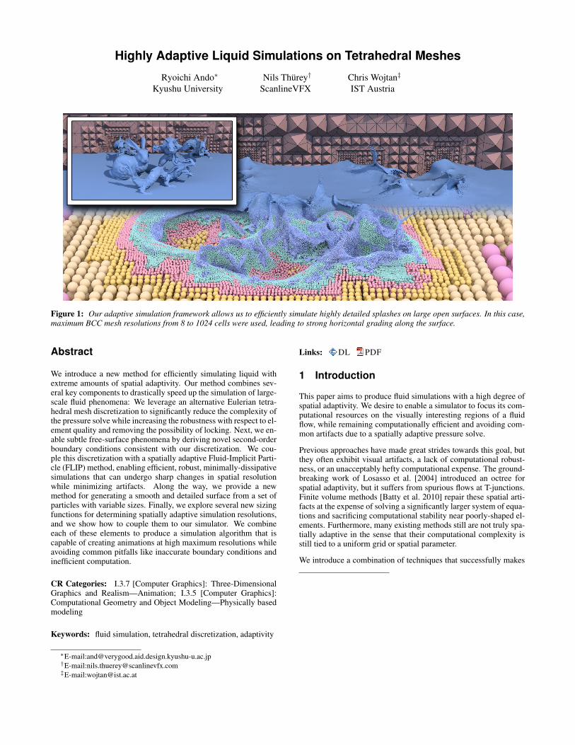
Figure 2: Our discretization compared to previous approaches:the MAC grid stores velocity components normal to faces and pres-sure values at the center. The FVM discretizations follow alongthese lines and store velocities normal to faces and pressure val-ues at the circumcenter of a cell. In our approach we store a 3-component velocity vector at the barycenter of a cell and pressurevalues at each node.

where V denotes a matrix containing the Vi as diagonal entries.The [∇]T [∇] matrix-matrix multiplication results in a square n×nmatrix, which is symmetric and positive definite. In the following,we will denote the matrix on the left hand side of Eq. (4) as A.Given appropriate boundary conditions, we can use standard tools,such as a commonly used pre-conditioned conjugate gradient solverto compute a solution (we use the one suggested in [Bridson 2008]).

Now, all that is left to construct the left-hand side matrix and theright-hand side terms for Eq. (4) is to define [∇]. As we assumea linear change of the pressure for each cell, we can use simplebarycentric interpolation to retrieve the pressure p at a position in-side a cell. Given the nodal pressure values p1..4 and barycentricweights σ1..4 this means p = σ1p1 + σ2p2 + σ3p3 + σ4p4. Inline with finite element methods using linear elements, we definethe gradient based on the partial derivatives of the barycentric in-terpolation. E.g., the first component of the gradient for a cell iscomputed with

∂

∂xp =

∂σ1

∂xp1 +

∂σ2

∂xp2 +

∂σ3

∂xp3 +

∂σ4

∂xp4 . (5)

To set up the final linear system of Eq. (4) for the pressure solve, weloop over all tetrahedra to compute the derivatives of the barycentricinterpolation, adding their contributions to the global matrix.

In contrast to previous work, our pressure solve is a linear systemthat has n degrees of freedom, n being the number of nodes inthe tetrahedral mesh. For our BCC mesh, n is in practice smallerthan the number of tetrahedra m (by a factor of 6 on average). Adirect implication of this smaller linear system is that it is fasterto solve. A second, less obvious implication of the smaller lin-ear system is that it effectively prevents artifacts known as locking.These artifacts are commonly observed in finite element methodsfor problems in elasticity. Different methods have been proposedto circumvent these problems, e.g., using linear elements for pres-sure instead of piece-wise constant ones [Irving et al. 2007]. Otherworks explicitly smooth the pressure field to reduce locking prob-lems [Misztal et al. 2010]. In general, locking can be observed if thepressure basis can represent more, and higher-frequency, functionsthan the basis for the velocity. Thus, choosing a more restrictivebasis for pressure, as in [Irving et al. 2007], or explicitly removinghigh-frequency information from the pressure [Misztal et al. 2010],reduces the chance of locking. Our method, by construction, hasmore degrees of freedom for representing velocity fields than pres-sure fields. Although we cannot prove that a local configurationover-constraining the velocities will never occur, the larger numberof degrees of freedom for our velocities effectively prevents lockingartifacts, and we have not encountered any in our tests.

Boundary Conditions Second-order boundary conditions are acentral component for accurate and visually appealing simulationswith non-conforming grids. Achieving second-order accuracy for

obstacle boundary conditions is straightforward with our discretiza-tion: we can rely on the formulation of previous work [Batty et al.2007], and set the volume of a cell Vi in Eq. (4) to the volume thatis filled with fluid.

For the free surface, we have to ensure that the Dirichlet boundarycondition p = 0 is satisfied at the interface position. Usually, thismeans computing a pressure value for nodes outside of the liquidso that a linear interpolation along an edge of a cell gives zero atthe correct position [Enright et al. 2005; Lew and Buscaglia 2008].Considering two pressure samples along an edge, we’ll denote val-ues inside the air with a G subscript, and values inside the liquidwith an L subscript in the following. For a Cartesian MAC grid, theghost pressure value pG is given by pG = pLφG/φL. In our case,however, this approach does not yield the desired result. The reasonis that our velocity samples are not in line with the direct connec-tions of the pressure samples – they are not locally orthogonal toeach other. Instead, we have to ensure the boundary conditions re-sult in the correct pressure value at the cell center. In the followingwe will show how to derive suitable free-surface boundary condi-tions to ensure second-order accuracy within our framework.

In order to achieve accurate and smooth surface motions with ourmethod, we compute the ghost pressure values pG with a linearcombination of liquid pressure values as:

pG = w1p1 + w2p2 + w3p3 , (6)

where wn and pn denote unknown coefficients and adjacent liquidpressures in the same tetrahedron. Note that for pi that are notinside of the liquid, we set wi = 0. In line with the traditionalghost fluid method, we define pG uniquely for each tetrahedron. Tohandle the most general case, let’s suppose that p1..3 are all liquidpressure values. Once we have a value for pG, we can compute apressure gradient for the tetrahedron and update the velocity at itscenter with:

unew = u∗ − ∆t

ρ[∇][pG p1 p2 p3

]T (7)

In order to do this we need to compute the coefficients wn. pGcan be rewritten in terms of a barycentric interpolation of the threevalues in the liquid as:

pG = pLφG/φL (8)

with φL = θ1φ1 + θ2φ2 + θ3φ3, and pL = θ1p1 + θ2p2 + θ3p3.Here the θn are a set of barycentric coordinate coefficients such thatθ1+θ2+θ3 = 1, and a tilde superscript denotes a value interpolatedwith the barycentric weights. Substituting Eq.8 into Eq.6 yields

wn = θnφG/φL . (9)

That means the values wn are determined by those of the θn coef-ficients, which we will compute in the following. Note that, theo-retically, θn could take any values as long as they add up to one.Before embedding the boundary conditions, the matrix entries ofthe pressure solve for a single tetrahedron are, according to Eq. (4),given by ∆t

ρ[∇]TV [∇]p = b. The computation of the ghost fluid

values is independent of the right-hand side b, so we will restrictthe discussion to the left hand side. We denote the components ofthe local symmetric 4× 4 matrix on the left hand side with:λ1 α β γ

α λ2 a bβ a λ3 cγ b c λ4

(10)

Assuming, without loss of generality, that the first vertex is the oneoutside of the liquid volume, we embed the boundary condition into

M based on the wn coefficients. Then the first row of the system ischanged to:1 −w1 −w2 −w3

α λ2 a bβ a λ3 cγ b c λ4

pGp1

p2

p3

=

0b1b2b3

. (11)

We can extract two constraints for each θn from this form, which,together with the barycentric coefficient constraint, give us a 3× 3matrix M ′ that can be inverted analytically. A full derivation ofthese steps can be found in Appendix A. With this analytic expres-sion we can compute the ghost pressure coefficients as:

w =φG/φL

α+ β + γ

αβγ

(12)

This boundary condition ensures second-order accuracy whilemaintaining symmetry when it is assembled into the matrix ofEq. (4). If the quality of a tetrahedron is good, 0 < θn < 1 isguaranteed. In this case, the resulting matrix is symmetric positive-definite and can be easily inverted by the commonly used precondi-tioned conjugate gradient methods. However, positive off-diagonalterms of the matrix can result in values of θ outside of the range[0, 1], leading to an indefinite linear system. In these cases we con-sider the tetrahedron to have a poor quality. When using ghost fluidboundary conditions with a regular MAC grid, it is common prac-tice to clamp small values in the denominator of Eq. (9) to preventill-conditioned pressure matrices. Effectively, this means revertingto first-order accuracy when second-order accuracy is intractable.We implement a similar step in our algorithm to overcome numeri-cal problems resulting from badly shaped cells. We check whetherthe ghost fluid boundary conditions would violate diagonal domi-nance of an equation in our linear system. If we detect such a case,we smoothly transition to first order accuracy. Specifically, whenwe have computed M ′, we check if a resulting diagonal term M ′i,iis smaller than ϕλ2..4. Here, ϕ denotes a tolerance factor that weset to ϕ = 0.25. Whenever we detect such a case, we compute acoefficient k with

k = min(ϕ− 1

w2αλ2,

ϕ− 1

w3βλ3,

ϕ− 1

w4γλ4

), (13)

and multiply each wn with k when embedding. Note that this scal-ing does not break the symmetry of the resulting linear system.More specifically, for k = 1 this yields full second-order accuracy,while for badly shaped tetrahedra the resulting k = 0 means thatwe revert to the standard rounding strategy of a first order accuratemethod. With our BCC mesh, all regular BCC tetrahedra have verygood quality and valid θn values. The graded BCC tetrahedra, onthe other hand, can be of lower quality and can require the use ofEq. (13). Luckily, in our tests these tetrahedra make up only a verysmall fraction of the mesh.

Velocity Interpolation The FLIP advection step traces particlesbased on the velocities from the Eulerian grid. For this we need toconstruct a continuous velocity field based on the discrete valuesin our tetrahedral mesh. As we store velocities at the cell centers,the interpolation would ideally use the dual mesh consisting of theVoronoi cells of each node [Brochu et al. 2010]. Unfortunately,performing interpolations within arbitrary Voronoi cells would beexpensive and require a large amount of computation compared tothe other steps of our simulator. Instead, we have found the fol-lowing approach to yield high speed and good accuracy: we firstinterpolate the centered velocities to the nodes, similar to [Chen-tanez et al. 2007]. Instead of interpolating these averaged values

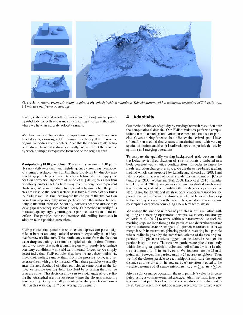
Figure 3: A simple geometric setup creating a big splash inside a container. This simulation, with a maximum resolution of 256 cells, took1.3 minutes per frame on average.

directly (which would result in smeared out motion), we temporar-ily subdivide the cells of our mesh by inserting a vertex at the centerwhere we have an accurate velocity sample.

We then perform barycentric interpolation based on these sub-divided cells, ensuring a C0 continuous velocity that retains theoriginal velocities at cell centers. Note that these four smaller tetra-hedra do not have to be stored explicitly. We construct them on thefly when a sample is requested from one of the original cells.

Manipulating FLIP particles The spacing between FLIP parti-cles may drift over time, and high-frequency errors may contributeto a bumpy surface. We combat these problems by directly ma-nipulating particle positions. During each time step, we apply theposition correction algorithm of Ando et al. [2012]; this algorithmessentially pushes each particle away from its neighbors to preventclustering. We also introduce two special behaviors when the parti-cles are close to the liquid surface (less than a distance of six timesthe particle radius). First, we impose the constraint that the positioncorrection step may only move particles near the surface tangen-tially to the fluid interface. Secondly, particles near the surface mayleave gaps when they spread out quickly. Our method naturally fillsin these gaps by slightly pulling each particle towards the fluid in-terface. For particles near the interface, this pulling force acts inaddition to the position correction.

FLIP particles that partake in splashes and sprays can pose a sig-nificant burden on computational resources, especially in an adap-tive framework like ours. This inefficiency stems from the fact thatwater droplets undergo extremely simple ballistic motion. Theoret-ically, we know that such a small region with purely free-surfaceboundary conditions will yield zero internal forces, so we simplydetect individual FLIP particles that have no neighbors within sixtimes their radius, remove them from the pressure solve, and ac-celerate them with gravity instead. When these particles eventuallyenter the neighborhood of other particles at some point in the fu-ture, we resume treating them like fluid by returning them to thepressure solve. This decision allows us to avoid aggressively refin-ing the tetrahedral mesh in locations where the physical motion isuninteresting. Only a small percentage of the particles are simu-lated in this way, e.g., 1.7% on average for Figure 6.

4 Adaptivity

Our method achieves adaptivity by varying the mesh resolution overthe computational domain. Our FLIP simulation performs compu-tation on both a background volumetric mesh and on a set of parti-cles. Given a sizing function that indicates the desired spatial levelof detail, our method first creates a tetrahedral mesh with varyingspatial resolution, and then it locally changes the particle density bysplitting and merging operations.

To compute the spatially-varying background grid, we start withthe Delaunay tetrahedralization of a set of points distributed in abody-centered cubic lattice configuration. In order to make themesh resolution change over space, we use the octree-based gradingmethod which was proposed by Labelle and Shewchuk [2007] andlater adopted in several adaptive simulation environments [Chen-tanez et al. 2007; Wojtan and Turk 2008; Batty et al. 2010]. Similarto [Batty et al. 2010], we generate a new tetrahedral mesh everyten time steps, instead of rebuilding the mesh on every consecutivestep. Also, the tetrahedral mesh is only temporarily used for thepressure solver, so no information is transferred from one time stepto the next by storing it on the grid. Thus, we do not worry aboutre-sampling data when computing a new tetrahedral mesh.

We change the size and number of particles in our simulation withsplitting and merging operations. For this, we modify the strategyof Ando et al. [2012] to work within our framework: at each re-meshing step, we loop through the particles and determine whetherthe resolution needs to be changed. If a particle is too small, then wemerge it with its nearest neighboring particle, resulting in a particlewhose radius is given by the combined volume of the two originalparticles. If a given particle is bigger than the desired size, then theparticle is split in two. The two new particles are placed randomlywithin the original particle’s radius and redistributed with a heuris-tic that attempts to fill in nearby gaps: We first compute the 24 mid-points mi between this particle and its 24 nearest neighbors. Thenwe find the closest particle to each midpoint and store the squareddistance as a weight ωi. The new particle’s position is equal to theweighted average of all nearby midpoints: xnew =

∑ωimi/

∑ωi.

After a split or merge operation, the new particle’s velocity is com-puted using a volume-weighted average. Also, we must take careto ensure that particles close to the surface do not introduce inter-facial bumps when they split or merge; whenever we create a new

a) c)b) d) e)

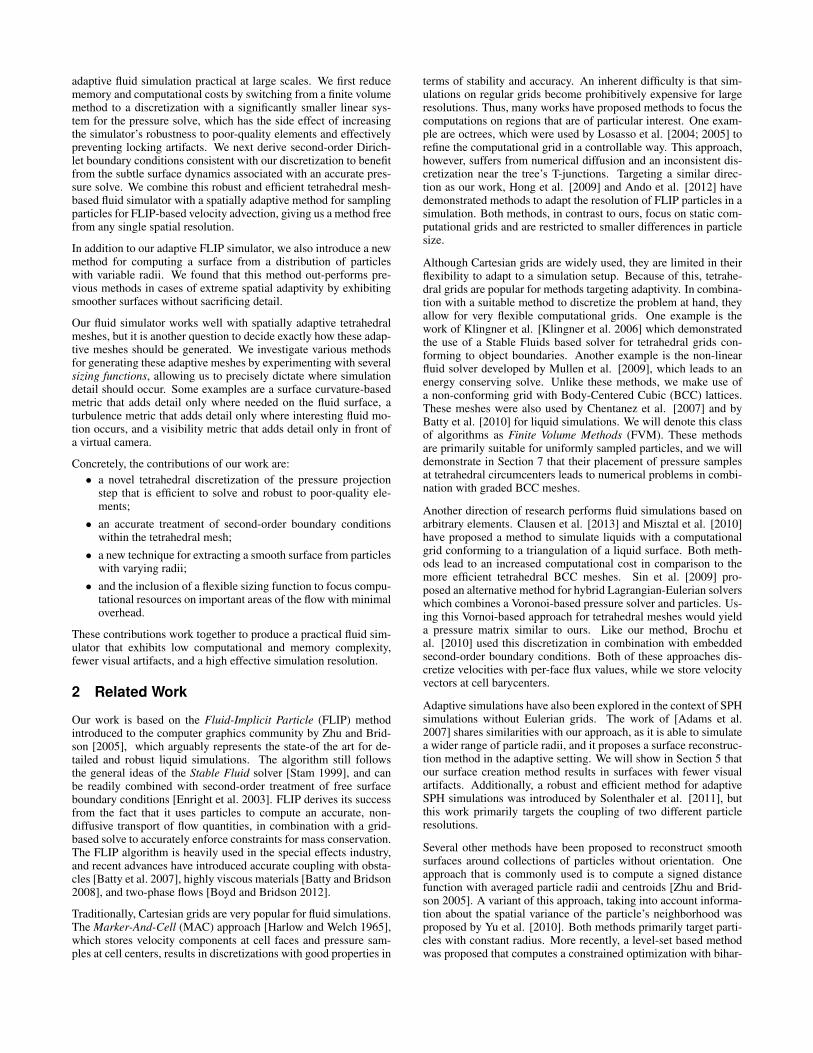
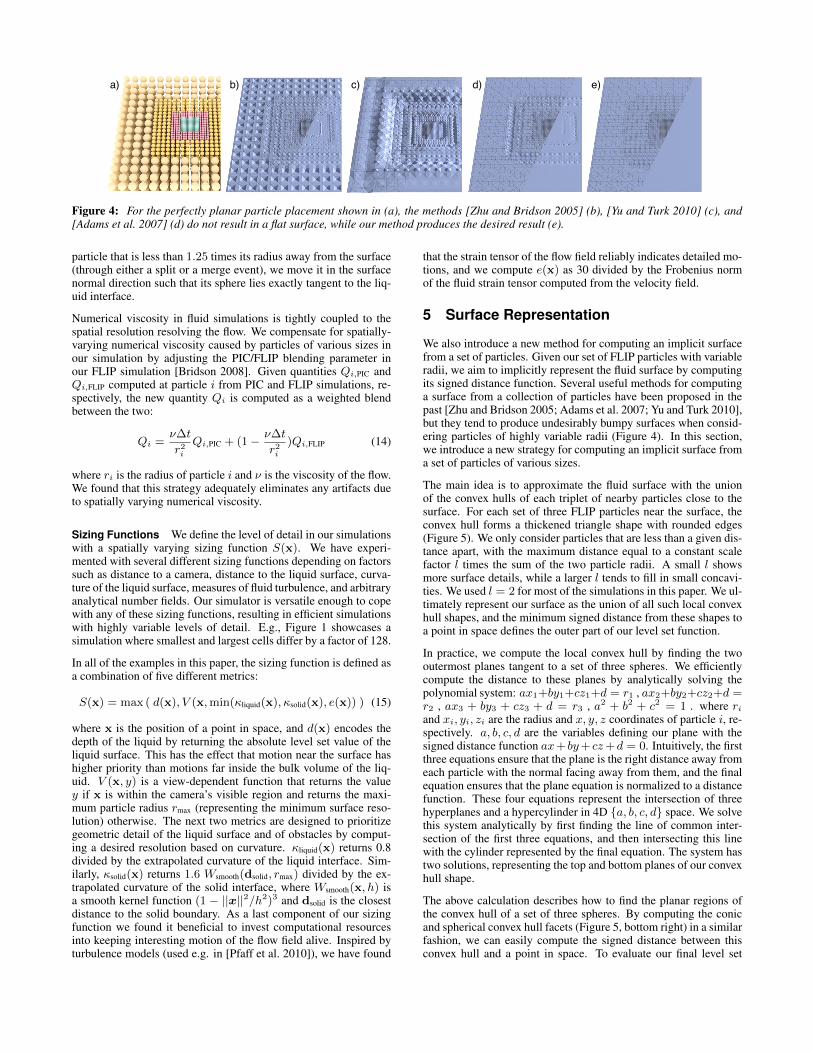
Figure 4: For the perfectly planar particle placement shown in (a), the methods [Zhu and Bridson 2005] (b), [Yu and Turk 2010] (c), and[Adams et al. 2007] (d) do not result in a flat surface, while our method produces the desired result (e).

particle that is less than 1.25 times its radius away from the surface(through either a split or a merge event), we move it in the surfacenormal direction such that its sphere lies exactly tangent to the liq-uid interface.

Numerical viscosity in fluid simulations is tightly coupled to thespatial resolution resolving the flow. We compensate for spatially-varying numerical viscosity caused by particles of various sizes inour simulation by adjusting the PIC/FLIP blending parameter inour FLIP simulation [Bridson 2008]. Given quantities Qi,PIC andQi,FLIP computed at particle i from PIC and FLIP simulations, re-spectively, the new quantity Qi is computed as a weighted blendbetween the two:

Qi =ν∆t

r2i

Qi,PIC + (1− ν∆t

r2i

)Qi,FLIP (14)

where ri is the radius of particle i and ν is the viscosity of the flow.We found that this strategy adequately eliminates any artifacts dueto spatially varying numerical viscosity.

Sizing Functions We define the level of detail in our simulationswith a spatially varying sizing function S(x). We have experi-mented with several different sizing functions depending on factorssuch as distance to a camera, distance to the liquid surface, curva-ture of the liquid surface, measures of fluid turbulence, and arbitraryanalytical number fields. Our simulator is versatile enough to copewith any of these sizing functions, resulting in efficient simulationswith highly variable levels of detail. E.g., Figure 1 showcases asimulation where smallest and largest cells differ by a factor of 128.

In all of the examples in this paper, the sizing function is defined asa combination of five different metrics:

S(x) = max ( d(x), V (x,min(κliquid(x), κsolid(x), e(x)) ) (15)

where x is the position of a point in space, and d(x) encodes thedepth of the liquid by returning the absolute level set value of theliquid surface. This has the effect that motion near the surface hashigher priority than motions far inside the bulk volume of the liq-uid. V (x, y) is a view-dependent function that returns the valuey if x is within the camera’s visible region and returns the maxi-mum particle radius rmax (representing the minimum surface reso-lution) otherwise. The next two metrics are designed to prioritizegeometric detail of the liquid surface and of obstacles by comput-ing a desired resolution based on curvature. κliquid(x) returns 0.8divided by the extrapolated curvature of the liquid interface. Sim-ilarly, κsolid(x) returns 1.6 Wsmooth(dsolid, rmax) divided by the ex-trapolated curvature of the solid interface, where Wsmooth(x, h) isa smooth kernel function (1 − ||x||2/h2)3 and dsolid is the closestdistance to the solid boundary. As a last component of our sizingfunction we found it beneficial to invest computational resourcesinto keeping interesting motion of the flow field alive. Inspired byturbulence models (used e.g. in [Pfaff et al. 2010]), we have found

that the strain tensor of the flow field reliably indicates detailed mo-tions, and we compute e(x) as 30 divided by the Frobenius normof the fluid strain tensor computed from the velocity field.

5 Surface Representation

We also introduce a new method for computing an implicit surfacefrom a set of particles. Given our set of FLIP particles with variableradii, we aim to implicitly represent the fluid surface by computingits signed distance function. Several useful methods for computinga surface from a collection of particles have been proposed in thepast [Zhu and Bridson 2005; Adams et al. 2007; Yu and Turk 2010],but they tend to produce undesirably bumpy surfaces when consid-ering particles of highly variable radii (Figure 4). In this section,we introduce a new strategy for computing an implicit surface froma set of particles of various sizes.

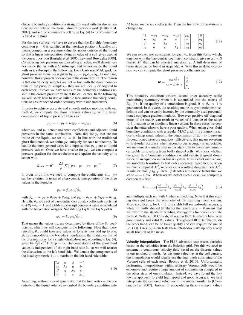
The main idea is to approximate the fluid surface with the unionof the convex hulls of each triplet of nearby particles close to thesurface. For each set of three FLIP particles near the surface, theconvex hull forms a thickened triangle shape with rounded edges(Figure 5). We only consider particles that are less than a given dis-tance apart, with the maximum distance equal to a constant scalefactor l times the sum of the two particle radii. A small l showsmore surface details, while a larger l tends to fill in small concavi-ties. We used l = 2 for most of the simulations in this paper. We ul-timately represent our surface as the union of all such local convexhull shapes, and the minimum signed distance from these shapes toa point in space defines the outer part of our level set function.

In practice, we compute the local convex hull by finding the twooutermost planes tangent to a set of three spheres. We efficientlycompute the distance to these planes by analytically solving thepolynomial system: ax1+by1+cz1+d = r1 , ax2+by2+cz2+d =r2 , ax3 + by3 + cz3 + d = r3 , a2 + b2 + c2 = 1 . where riand xi, yi, zi are the radius and x, y, z coordinates of particle i, re-spectively. a, b, c, d are the variables defining our plane with thesigned distance function ax+ by+ cz+d = 0. Intuitively, the firstthree equations ensure that the plane is the right distance away fromeach particle with the normal facing away from them, and the finalequation ensures that the plane equation is normalized to a distancefunction. These four equations represent the intersection of threehyperplanes and a hypercylinder in 4D a, b, c, d space. We solvethis system analytically by first finding the line of common inter-section of the first three equations, and then intersecting this linewith the cylinder represented by the final equation. The system hastwo solutions, representing the top and bottom planes of our convexhull shape.

The above calculation describes how to find the planar regions ofthe convex hull of a set of three spheres. By computing the conicand spherical convex hull facets (Figure 5, bottom right) in a similarfashion, we can easily compute the signed distance between thisconvex hull and a point in space. To evaluate our final level set

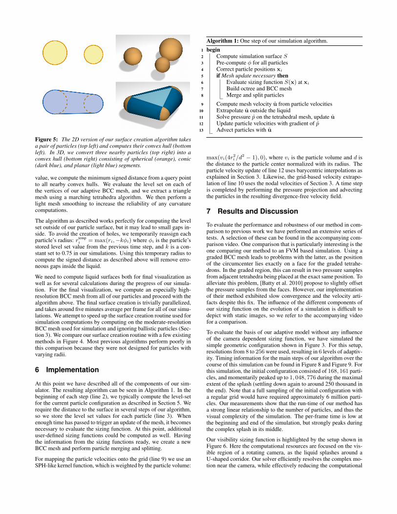
Figure 5: The 2D version of our surface creation algorithm takesa pair of particles (top left) and computes their convex hull (bottomleft). In 3D, we convert three nearby particles (top right) into aconvex hull (bottom right) consisting of spherical (orange), conic(dark blue), and planar (light blue) segments.

value, we compute the minimum signed distance from a query pointto all nearby convex hulls. We evaluate the level set on each ofthe vertices of our adaptive BCC mesh, and we extract a trianglemesh using a marching tetrahedra algorithm. We then perform alight mesh smoothing to increase the reliability of any curvaturecomputations.

The algorithm as described works perfectly for computing the levelset outside of our particle surface, but it may lead to small gaps in-side. To avoid the creation of holes, we temporarily reassign eachparticle’s radius: rtemp

i = max(ri,−kφi) where φi is the particle’sstored level set value from the previous time step, and k is a con-stant set to 0.75 in our simulations. Using this temporary radius tocompute the signed distance as described above will remove erro-neous gaps inside the liquid.

We need to compute liquid surfaces both for final visualization aswell as for several calculations during the progress of our simula-tion. For the final visualization, we compute an especially high-resolution BCC mesh from all of our particles and proceed with thealgorithm above. The final surface creation is trivially parallelized,and takes around five minutes average per frame for all of our simu-lations. We attempt to speed up the surface creation routine used forsimulation computations by computing on the moderate-resolutionBCC mesh used for simulation and ignoring ballistic particles (Sec-tion 3). We compare our surface creation routine with a few existingmethods in Figure 4. Most previous algorithms perform poorly inthis comparison because they were not designed for particles withvarying radii.

6 Implementation

At this point we have described all of the components of our sim-ulator. The resulting algorithm can be seen in Algorithm 1. In thebeginning of each step (line 2), we typically compute the level-setfor the current particle configuration as described in Section 5. Werequire the distance to the surface in several steps of our algorithm,so we store the level set values for each particle (line 3). Whenenough time has passed to trigger an update of the mesh, it becomesnecessary to evaluate the sizing function. At this point, additionaluser-defined sizing functions could be computed as well. Havingthe information from the sizing functions ready, we create a newBCC mesh and perform particle merging and splitting.

For mapping the particle velocities onto the grid (line 9) we use anSPH-like kernel function, which is weighted by the particle volume:

Algorithm 1: One step of our simulation algorithm.

1 begin2 Compute simulation surface S3 Pre-compute φ for all particles4 Correct particle positions xi5 if Mesh update necessary then6 Evaluate sizing function S(x) at xi7 Build octree and BCC mesh8 Merge and split particles

9 Compute mesh velocity u from particle velocities10 Extrapolate u outside the liquid11 Solve pressure p on the tetrahedral mesh, update u12 Update particle velocities with gradient of p13 Advect particles with u

max(vi(4r2i /d

2 − 1), 0), where vi is the particle volume and d isthe distance to the particle center normalized with its radius. Theparticle velocity update of line 12 uses barycentric interpolations asexplained in Section 3. Likewise, the grid-based velocity extrapo-lation of line 10 uses the nodal velocities of Section 3. A time stepis completed by performing the pressure projection and advectingthe particles in the resulting divergence-free velocity field.

7 Results and Discussion

To evaluate the performance and robustness of our method in com-parison to previous work we have performed an extensive series oftests. A selection of these can be found in the accompanying com-parison video. One comparison that is particularly interesting is theone comparing our method to an FVM based simulation. Using agraded BCC mesh leads to problems with the latter, as the positionof the circumcenter lies exactly on a face for the graded tetrahe-drons. In the graded region, this can result in two pressure samplesfrom adjacent tetrahedra being placed at the exact same position. Toalleviate this problem, [Batty et al. 2010] propose to slightly offsetthe pressure samples from the faces. However, our implementationof their method exhibited slow convergence and the velocity arti-facts despite this fix. The influence of the different components ofour sizing function on the evolution of a simulation is difficult todepict with static images, so we refer to the accompanying videofor a comparison.

To evaluate the basis of our adaptive model without any influenceof the camera dependent sizing function, we have simulated thesimple geometric configuration shown in Figure 3. For this setup,resolutions from 8 to 256 were used, resulting in 6 levels of adaptiv-ity. Timing information for the main steps of our algorithm over thecourse of this simulation can be found in Figure 8 and Figure 9. Forthis simulation, the initial configuration consisted of 168, 161 parti-cles, and momentarily peaked up to 1, 048, 776 during the maximalextent of the splash (settling down again to around 250 thousand inthe end). Note that a full sampling of the initial configuration witha regular grid would have required approximately 6 million parti-cles. Our measurements show that the run-time of our method hasa strong linear relationship to the number of particles, and thus thevisual complexity of the simulation. The per-frame time is low atthe beginning and end of the simulation, but strongly peaks duringthe complex splash in its middle.

Our visibility sizing function is highlighted by the setup shown inFigure 6. Here the computational resources are focused on the vis-ible region of a rotating camera, as the liquid splashes around aU-shaped corridor. Our solver efficiently resolves the complex mo-tion near the camera, while effectively reducing the computational

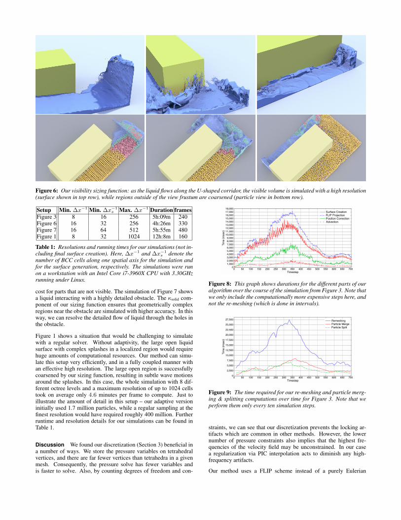
Figure 6: Our visibility sizing function: as the liquid flows along the U-shaped corridor, the visible volume is simulated with a high resolution(surface shown in top row), while regions outside of the view frustum are coarsened (particle view in bottom row).

Setup Min. ∆x−1 Min. ∆x−1s Max. ∆x−1 Duration frames

Figure 3 8 16 256 5h:09m 240Figure 6 16 32 256 4h:26m 330Figure 7 16 64 512 5h:55m 480Figure 1 8 32 1024 12h:8m 160

Table 1: Resolutions and running times for our simulations (not in-cluding final surface creation). Here, ∆x−1 and ∆x−1

s denote thenumber of BCC cells along one spatial axis for the simulation andfor the surface generation, respectively. The simulations were runon a workstation with an Intel Core i7-3960X CPU with 3.30GHzrunning under Linux.

cost for parts that are not visible. The simulation of Figure 7 showsa liquid interacting with a highly detailed obstacle. The κsolid com-ponent of our sizing function ensures that geometrically complexregions near the obstacle are simulated with higher accuracy. In thisway, we can resolve the detailed flow of liquid through the holes inthe obstacle.

Figure 1 shows a situation that would be challenging to simulatewith a regular solver. Without adaptivity, the large open liquidsurface with complex splashes in a localized region would requirehuge amounts of computational resources. Our method can simu-late this setup very efficiently, and in a fully coupled manner withan effective high resolution. The large open region is successfullycoarsened by our sizing function, resulting in subtle wave motionsaround the splashes. In this case, the whole simulation with 8 dif-ferent octree levels and a maximum resolution of up to 1024 cellstook on average only 4.6 minutes per frame to compute. Just toillustrate the amount of detail in this setup – our adaptive versioninitially used 1.7 million particles, while a regular sampling at thefinest resolution would have required roughly 400 million. Furtherruntime and resolution details for our simulations can be found inTable 1.

Discussion We found our discretization (Section 3) beneficial ina number of ways. We store the pressure variables on tetrahedralvertices, and there are far fewer vertices than tetrahedra in a givenmesh. Consequently, the pressure solve has fewer variables andis faster to solve. Also, by counting degrees of freedom and con-

Figure 8: This graph shows durations for the different parts of ouralgorithm over the course of the simulation from Figure 3. Note thatwe only include the computationally more expensive steps here, andnot the re-meshing (which is done in intervals).

Figure 9: The time required for our re-meshing and particle merg-ing & splitting computations over time for Figure 3. Note that weperform them only every ten simulation steps.

straints, we can see that our discretization prevents the locking ar-tifacts which are common in other methods. However, the lowernumber of pressure constraints also implies that the highest fre-quencies of the velocity field may be unconstrained. In our casea regularization via PIC interpolation acts to diminish any high-frequency artifacts.

Our method uses a FLIP scheme instead of a purely Eulerian

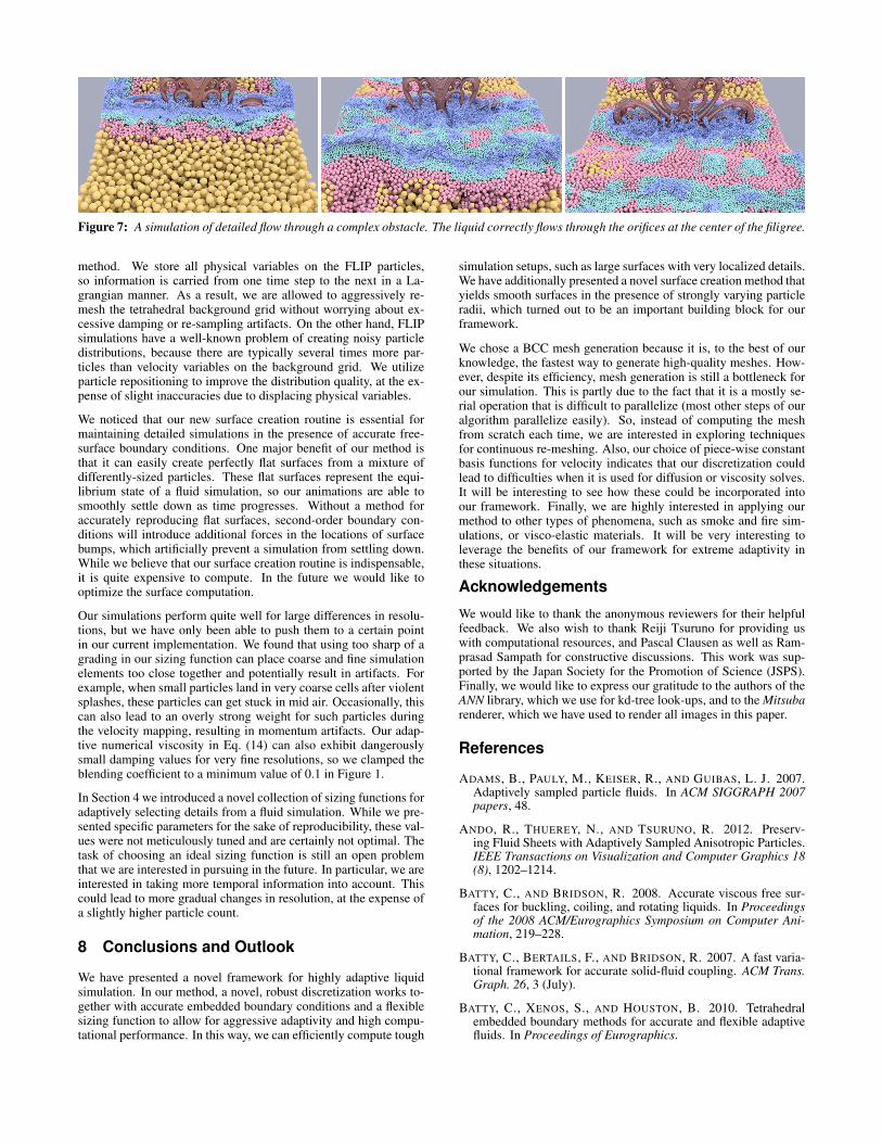
Figure 7: A simulation of detailed flow through a complex obstacle. The liquid correctly flows through the orifices at the center of the filigree.

method. We store all physical variables on the FLIP particles,so information is carried from one time step to the next in a La-grangian manner. As a result, we are allowed to aggressively re-mesh the tetrahedral background grid without worrying about ex-cessive damping or re-sampling artifacts. On the other hand, FLIPsimulations have a well-known problem of creating noisy particledistributions, because there are typically several times more par-ticles than velocity variables on the background grid. We utilizeparticle repositioning to improve the distribution quality, at the ex-pense of slight inaccuracies due to displacing physical variables.

We noticed that our new surface creation routine is essential formaintaining detailed simulations in the presence of accurate free-surface boundary conditions. One major benefit of our method isthat it can easily create perfectly flat surfaces from a mixture ofdifferently-sized particles. These flat surfaces represent the equi-librium state of a fluid simulation, so our animations are able tosmoothly settle down as time progresses. Without a method foraccurately reproducing flat surfaces, second-order boundary con-ditions will introduce additional forces in the locations of surfacebumps, which artificially prevent a simulation from settling down.While we believe that our surface creation routine is indispensable,it is quite expensive to compute. In the future we would like tooptimize the surface computation.

Our simulations perform quite well for large differences in resolu-tions, but we have only been able to push them to a certain pointin our current implementation. We found that using too sharp of agrading in our sizing function can place coarse and fine simulationelements too close together and potentially result in artifacts. Forexample, when small particles land in very coarse cells after violentsplashes, these particles can get stuck in mid air. Occasionally, thiscan also lead to an overly strong weight for such particles duringthe velocity mapping, resulting in momentum artifacts. Our adap-tive numerical viscosity in Eq. (14) can also exhibit dangerouslysmall damping values for very fine resolutions, so we clamped theblending coefficient to a minimum value of 0.1 in Figure 1.

In Section 4 we introduced a novel collection of sizing functions foradaptively selecting details from a fluid simulation. While we pre-sented specific parameters for the sake of reproducibility, these val-ues were not meticulously tuned and are certainly not optimal. Thetask of choosing an ideal sizing function is still an open problemthat we are interested in pursuing in the future. In particular, we areinterested in taking more temporal information into account. Thiscould lead to more gradual changes in resolution, at the expense ofa slightly higher particle count.

8 Conclusions and Outlook

We have presented a novel framework for highly adaptive liquidsimulation. In our method, a novel, robust discretization works to-gether with accurate embedded boundary conditions and a flexiblesizing function to allow for aggressive adaptivity and high compu-tational performance. In this way, we can efficiently compute tough

simulation setups, such as large surfaces with very localized details.We have additionally presented a novel surface creation method thatyields smooth surfaces in the presence of strongly varying particleradii, which turned out to be an important building block for ourframework.

We chose a BCC mesh generation because it is, to the best of ourknowledge, the fastest way to generate high-quality meshes. How-ever, despite its efficiency, mesh generation is still a bottleneck forour simulation. This is partly due to the fact that it is a mostly se-rial operation that is difficult to parallelize (most other steps of ouralgorithm parallelize easily). So, instead of computing the meshfrom scratch each time, we are interested in exploring techniquesfor continuous re-meshing. Also, our choice of piece-wise constantbasis functions for velocity indicates that our discretization couldlead to difficulties when it is used for diffusion or viscosity solves.It will be interesting to see how these could be incorporated intoour framework. Finally, we are highly interested in applying ourmethod to other types of phenomena, such as smoke and fire sim-ulations, or visco-elastic materials. It will be very interesting toleverage the benefits of our framework for extreme adaptivity inthese situations.

Acknowledgements

We would like to thank the anonymous reviewers for their helpfulfeedback. We also wish to thank Reiji Tsuruno for providing uswith computational resources, and Pascal Clausen as well as Ram-prasad Sampath for constructive discussions. This work was sup-ported by the Japan Society for the Promotion of Science (JSPS).Finally, we would like to express our gratitude to the authors of theANN library, which we use for kd-tree look-ups, and to the Mitsubarenderer, which we have used to render all images in this paper.

References

ADAMS, B., PAULY, M., KEISER, R., AND GUIBAS, L. J. 2007.Adaptively sampled particle fluids. In ACM SIGGRAPH 2007papers, 48.

ANDO, R., THUEREY, N., AND TSURUNO, R. 2012. Preserv-ing Fluid Sheets with Adaptively Sampled Anisotropic Particles.IEEE Transactions on Visualization and Computer Graphics 18(8), 1202–1214.

BATTY, C., AND BRIDSON, R. 2008. Accurate viscous free sur-faces for buckling, coiling, and rotating liquids. In Proceedingsof the 2008 ACM/Eurographics Symposium on Computer Ani-mation, 219–228.

BATTY, C., BERTAILS, F., AND BRIDSON, R. 2007. A fast varia-tional framework for accurate solid-fluid coupling. ACM Trans.Graph. 26, 3 (July).

BATTY, C., XENOS, S., AND HOUSTON, B. 2010. Tetrahedralembedded boundary methods for accurate and flexible adaptivefluids. In Proceedings of Eurographics.

BHATTACHARYA, H., GAO, Y., AND BARGTEIL, A. W. 2011.A level-set method for skinning animated particle data. In Pro-ceedings of the ACM SIGGRAPH/Eurographics Symposium onComputer Animation.

BOYD, L., AND BRIDSON, R. 2012. Multiflip for energetic two-phase fluid simulation. ACM Trans. Graph. 31, 2, 16:1–16:12.

BRIDSON, R. 2008. Fluid Simulation for Computer Graphics.AK Peters/CRC Press.

BROCHU, T., BATTY, C., AND BRIDSON, R. 2010. Matching fluidsimulation elements to surface geometry and topology. ACMTrans. Graph. 29, 4 (July), 47:1–47:9.

CHENTANEZ, N., FELDMAN, B. E., LABELLE, F., O’BRIEN,J. F., AND SHEWCHUK, J. R. 2007. Liquid simulation onlattice-based tetrahedral meshes. In Proceedings of the 2007ACM SIGGRAPH/Eurographics Symposium on Computer Ani-mation, Eurographics Association, 219–228.

CLAUSEN, P., WICKE, M., SHEWCHUK, J., AND O’BRIEN, J.2013. Simulating liquids and solid-liquid interactions with La-grangian meshes. ACM Trans. Graph..

ENRIGHT, D., NGUYEN, D., GIBOU, F., AND FEDKIW, R. 2003.Using the Particle Level Set Method and a Second Order Accu-rate Pressure Boundary Condition for Free-Surface Flows. Proc.of the 4th ASME-JSME Joint Fluids Engineering Conference.

ENRIGHT, D., LOSASSO, F., AND FEDKIW, R. 2005. A fastand accurate semi-Lagrangian particle level set method. Com-put. Struct. 83, 6-7, 479–490.

HARLOW, F., AND WELCH, E. 1965. Numerical calculation oftime-dependent viscous incompressible flow of fluid with freesurface. Phys. Fluids 8 (12), 2182–2189.

HONG, W., HOUSE, D. H., AND KEYSER, J. 2009. An adap-tive sampling approach to incompressible particle-based fluid. InTPCG, Eurographics Association, W. Tang and J. P. Collomosse,Eds., 69–76.

IRVING, G., SCHROEDER, C., AND FEDKIW, R. 2007. Vol-ume conserving finite element simulations of deformable mod-els. ACM Trans. Graph. 26, 3 (July).

KLINGNER, B. M., FELDMAN, B. E., CHENTANEZ, N., ANDO’BRIEN, J. F. 2006. Fluid animation with dynamic meshes.ACM Trans. Graph. 25, 3, 820–825.

LABELLE, F., AND SHEWCHUK, J. R. 2007. Isosurface stuffing:Fast tetrahedral meshes with good dihedral angles. ACM Trans.Graph. 26, 3 (July).

LEW, A. J., AND BUSCAGLIA, G. C. 2008. A discontinuous-galerkin-based immersed boundary method. International Jour-nal for Numerical Methods in Engineering 76, 4, 427–454.

LOSASSO, F., GIBOU, F., AND FEDKIW, R. 2004. Simulating wa-ter and smoke with an octree data structure. ACM Trans. Graph.23, 3 (Aug.), 457–462.

LOSASSO, F., FEDKIW, R., AND OSHER, S. 2005. Spatially adap-tive techniques for level set methods and incompressible flow.Computers and Fluids 35, 2006.

MISZTAL, M. K., BRIDSON, R., ERLEBEN, K., BÆRENTZEN,J. A., AND ANTON, F. 2010. Optimization-based fluid simula-tion on unstructured meshes. In VRIPHYS, Eurographics Asso-ciation, 11–20.

MULLEN, P., CRANE, K., PAVLOV, D., TONG, Y., AND DES-BRUN, M. 2009. Energy-preserving integrators for fluid anima-tion. ACM Trans. Graph. 28 (July), 38:1–38:8.

PFAFF, T., THUEREY, N., COHEN, J., TARIQ, S., AND GROSS,M. 2010. Scalable fluid simulation using anisotropic turbulenceparticles. In ACM Transactions on Graphics (TOG), vol. 29,ACM, 174.

SIN, F., BARGTEIL, A. W., AND HODGINS, J. K. 2009. A point-based method for animating incompressible flow. In Proceedingsof the ACM SIGGRAPH/Eurographics Symposium on ComputerAnimation.

SOLENTHALER, B., AND GROSS, M. 2011. Two-scale particlesimulation. ACM Trans. Graph. 30, 4 (July), 81:1–81:8.

STAM, J. 1999. Stable fluids. In Proceedings of SIGGRAPH ’99,ACM, 121–128.

WOJTAN, C., AND TURK, G. 2008. Fast viscoelastic behaviorwith thin features. ACM Trans. Graph. 27, 3, 1–8.

YU, J., AND TURK, G. 2010. Reconstructing surfaces of particle-based fluids using anisotropic kernels. In Proceedings of the2010 ACM SIGGRAPH/Eurographics Symposium on ComputerAnimation, Eurographics Association, 217–225.

ZHU, Y., AND BRIDSON, R. 2005. Animating sand as a fluid.ACM Trans. Graph. 24, 3 (July), 965–972.

A Ghost Fluid Coefficients

Here we describe how to compute the ghost fluid coefficients θngiven the 4× 4 pressure matrix entries of a single tetrahedron. Re-organizing Eq. (11) gives:[

λ2 + αw1 a+ αw2 b+ αw3

a+ βw1 λ3 + βw2 c+ βw3

b+ γw1 c+ γw2 λ4 + γw3

][p1

p2

p3

]=

[b1b2b3

]. (16)

Note that each of the θn has two degree of freedom, and thus eachwn also has two degrees of freedom. As we know that the result-ing matrix needs to be symmetric, which gives us the followingconstraints: a + αw2 = a + βw1, b + γw1 = b + αw3, andc+βw3 = c+ γw2. As the wn linearly depend on θn, that means:αθ2 = βθ1, γθ1 = αθ3, and βθ3 = γθ2. When we re-write theseconstraints in matrix form, and include the barycentric coordinateconstraint θ1 + θ2 + θ3 = 1 we get the following linear system:−β α 0

γ 0 −α0 −γ β1 1 1

[θ1

θ2

θ3

]=

0001

(17)

As the rank of top three rows of the matrix is 2, we can drop one ofthem. Removing the first row from the system gives us the follow-ing full-rank, 3× 3 matrix:[

γ 0 −α0 −γ β1 1 1

][θ1

θ2

θ3

]=

[001

](18)

The analytical solution of this system is:[θ1

θ2

θ3

]=

1

α+ β + γ

[αβγ

]. (19)

This means that for our discretization, the ghost pressure coeffi-cients θn are given by the tetrahedron’s matrix entries from Eq.10.More specifically, by those for the vertex that is located outside ofthe liquid, i.e., α, β and γ.

Substituting this equation into Eq.9 and Eq.6 yields the final equa-tion for the ghost pressure Eq. (12).