www.elsevier.com/locate/geomorph

Geomorphology 55 (2003) 363–380

High spatial resolution hyperspectral mapping of in-stream

habitats, depths, and woody debris in mountain streams

W. Andrew Marcusa,*, Carl J. Legleiterb, Richard J. Aspinallb,Joseph W. Boardmanc, Robert L. Crabtreed

aDepartment of Geography, University of Oregon, Eugene, OR 97403-1251, USAbDepartment of Earth Sciences, Montana State University, Bozeman, MT 59717, USA

cAnalytical Imaging and Geophysics, 4450 Arapahoe Ave, Suite 100, Boulder, CO 80303, USAdYellowstone Ecological Research Center, 7500 Jarmen Circle, Suite #2, Bozeman, MT 59715, USA

Received 29 January 2002; received in revised form 10 May 2002; accepted 10 March 2003

Abstract

This article evaluates the potential of 1-m resolution, 128-band hyperspectral imagery for mapping in-stream habitats,

depths, and woody debris in third- to fifth-order streams in the northern Yellowstone region. Maximum likelihood supervised

classification using principal component images provided overall classification accuracies for in-stream habitats (glides, riffles,

pools, and eddy drop zones) ranging from 69% for third-order streams to 86% for fifth-order streams. This scale dependency of

classification accuracy was probably driven by the greater proportion of transitional boundary areas in the smaller streams.

Multiple regressions of measured depths ( y) versus principal component scores (x1, x2,. . ., xn) generated R2 values ranging from

67% for high-gradient riffles to 99% for glides in a fifth-order reach. R2 values were lower in third-order reaches, ranging from

28% for runs and glides to 94% for pools. The less accurate depth estimates obtained for smaller streams probably resulted from

the relative increase in the number of mixed pixels, where a wide range of depths and surface turbulence occurred within a

single pixel. Matched filter (MF) mapping of woody debris generated overall accuracies of 83% in the fifth-order Lamar River.

Accuracy figures for the in-stream habitat and wood mapping may have been misleadingly low because the fine-resolution

imagery captured fine-scale variations not mapped by field teams, which in turn generated false ‘‘misclassifications’’ when the

image and field maps were compared.

The use of high spatial resolution hyperspectral (HSRH) imagery for stream mapping is limited by the need for clear water to

measure depth, by any tree cover obscuring the stream, and by the limited availability of airborne hyperspectral sensors.

Nonetheless, the high accuracies achieved in northern Yellowstone streams indicate that HSRH imagery can be a powerful tool

for watershed-wide mapping, monitoring, and modeling of streams.

D 2003 Elsevier Science B.V. All rights reserved.

Keywords: Remote sensing; In-stream habitat; Morphology; Woody debris; Depth; Mountain stream

0169-555X/03/$ - see front matter D 2003 Elsevier Science B.V. All righ

doi:10.1016/S0169-555X(03)00150-8

* Corresponding author. Fax: +1-541-346-2067.

E-mail address: marcus@oregon.uoregon.edu (W.A. Marcus).

1. Introduction

Mapping variations in stream habitat, water depth,

and woody debris throughout entire watersheds can be

ts reserved.

W.A. Marcus et al. / Geomorphology 55 (2003) 363–380364

notoriously difficult in mountain environments. The

paucity or absence of fine spatial resolution, basin-

wide maps of stream characteristics poses a major

obstacle to understanding how mountain stream pro-

cesses and responses are integrated into broader,

watershed-wide geomorphic systems and are modified

by human impacts.

High spatial resolution hyperspectral (HSRH)

imagery is a tool potentially capable of acquiring

detailed maps over a stream’s entire length. High

spatial resolution (V 5 m) provides the detail neces-

sary to capture key features in the narrow headwater

streams typical of mountain environments. The spec-

tral coverage and narrow bandwidths associated with

hyperspectral imagery (generally z 64 bands) allow

the user to differentiate features of interest that could

not be distinguished otherwise. This article evaluates

the ability of 1-m, 128-band imagery to map in-stream

habitats, stream depths, and woody debris in third- to

fifth-order streams of the northern Yellowstone

region. If a single remote sensing instrument could

be used to map this suite of features at watershed

scales, it would simplify data collection, improve

access to remote areas, reduce costs, and enable better

monitoring and modeling of river habitat in mountain

watersheds.

2. Previous research

The early applications of digital remote sensing

technology in the context of fluvial systems focused

on large rivers or reservoirs, where the water could be

clearly delineated using the coarse 10–80-m pixel

resolution available from satellites. Since approxi-

mately 1990, however, the development and accessi-

bility of airborne sensors (e.g., AVIRIS); improved

technology for converting film-based images to digital

form; and high spatial resolution satellite-based sen-

sors (e.g., IKONOS) have created new opportunities

for applying digital remote sensing to small streams

typical of mountain environments. Fourteen sensors

with spatial resolutions of V 5 m are scheduled for

launch by the year 2005 and imagery from nine of

these instruments will be commercially available

(Ustin and Costick, 2000).

Research on remote sensing of in-stream features

has largely focused on microhabitats, such as pools,

glides, and riffles—critical habitats for benthic fauna

(Orth and Maughan, 1983). These morphologic units

also provide a template for predicting where contam-

inants might accumulate in stream sediments (Ladd et

al., 1998). Hardy et al. (1994) found ‘‘close’’ agree-

ment between ground- and image-based maps of

hydraulic features such as pools, eddies, and runs on

the Green River, UT, using multispectral video

imagery at spatial resolutions of 0.25–3 m. In con-

trast, in the much smaller third- and fourth-order Soda

Butte and Cache Creeks of Montana and Wyoming,

Wright et al. (2000) obtained poor results using 4-

band, 1-m imagery to map stream habitats, with

standard supervised classification procedures produc-

ing overall accuracies ranging from 10% to 53%. The

inadequacy of their results was largely attributed to

coregistration problems, although the need for greater

spectral resolution was also noted. To avoid these

coregistration issues, Marcus (2002) mapped stream

microhabitats in the fifth-order Lamar River of

Wyoming directly to hardcopy printouts of 1-m,

128-band hyperspectral imagery to ensure a perfect

match between the classified imagery and field maps.

Marcus used a maximum likelihood classification

approach to achieve an overall classification accuracy

of 85%. Using the same imagery and the same field

data, Goovaerts (2002) was able to improve the in-

stream habitat classification accuracy to 99% using a

co-kriging classification scheme.

Both the improved spectral and enhanced spatial

resolution provided by HSRH imagery appear neces-

sary to accurately map in-stream habitats. Marcus

(2002) found that using 1 m rather than 5-m pixel

resolution increased overall accuracies by 19.4% and

that using 128 band rather than 4-band, 1-m imagery

improved accuracies by 17.6%. Similarly, Legleiter et

al. (2002) noted that overall accuracies increased by

7.2% when using 128-band HSRH imagery rather

than 8-band imagery and by 4.7% when using 1 m

rather than 2.5-m imagery.

Research on remote measurement of stream depth

has also received increasing attention from the remote

sensing community in recent years. Lyon et al. (1992)

classified five depth categories with 95% accuracy

using a radiative transfer model with four visible light

bands in the relatively large (compared to our study

sites) Saint Mary’s River of Michigan. The radiative

transfer model and resultant depth estimates, however,

W.A. Marcus et al. / Geomorphology 55 (2003) 363–380 365

were dependent on Secchi Disk measurements of

extinction coefficients, an approach that would be

difficult or impossible to apply in the comparatively

shallow and often turbulent conditions found in

mountain rivers. Gilvear et al. (1995) used scanned

panchromatic photos with f 1-m resolution to differ-

entiate deep versus shallow water, but did not attempt

precise depth estimates. A quantitative study by

Winterbottom and Gilvear (1997) succeeded in esti-

mating depths with 2-m, 9-band simulated Daedalus

AADS imagery, generating R2 values of 67% for

water depths up to 1.2 m. Their cross-section analysis

indicated that the 67% figure probably underrepre-

sented the quality of the depth estimates, which

produced cross-sections very similar to those sur-

veyed at the same sites.

Active sensors, including radar, have shown greater

potential for accurate depth measurements than have

passive, reflected signals. In a variety of stream con-

ditions with depths up to 5 m, ground-penetrating radar

produced an overall R2 value of 97% for measured

versus estimated depths (Spicer et al., 1997). Ground-

penetrating radar also shows great promise as a techni-

que for estimating stream velocities (Spicer et al., 1997;

Costa et al., 2000).

In comparison to work on microhabitats and stream

depth, remote sensing of wood has received relatively

little research attention. Marcus et al. (2002) had

relatively poor success using 1-m, 4-band imagery

to map wood in Cache Creek in northern Yellowstone

Park, largely because of spectral confusion between

gravel and wood in mixed pixels and coregistration

problems similar to those encountered by Wright et al.

(2000). Although readily apparent to the naked eye,

the configuration of woody debris (especially when

present as isolated logs or small sets of logs) made up

such small portions of individual pixels that it often

could not be distinguished from the surrounding

background, even with 1-m imagery. Marcus et al.

(2002) recommended using either finer resolution

imagery, which is difficult to acquire, or hyperspectral

imagery, which enables objects with a clear spectral

signal (like wood) to be distinguished even when they

make up only a fraction of a pixel (Boardman, 1989,

1993).

Previous research has demonstrated the potential of

digital remote sensing as a tool for mapping key

characteristics of small streams. To date, however,

the research has focused on using imagery to map one

variable, usually within a reach of limited size. Eval-

uating whether a single instrument can map a suite of

critical habitat characteristics indicates how effec-

tively these approaches can simplify and improve

watershed-wide mapping of streams. Quantifying var-

iations in mapping accuracy is also required to under-

stand the performance of these techniques at varying

stream scales. This article evaluates the potential for

using high spatial resolution hyperspectral imagery

(HSRH imagery) to map stream microhabitats and

depths in third-, fourth-, and fifth-order channels and

wood within and on the bars of a fifth-order channel.

3. Field area

We collected hyperspectral imagery and mapped

in-stream habitats and depths in August 1999 along

two reaches in Soda Butte Creek and one reach in the

Lamar River (Fig. 1). Because of time constraints,

woody debris was only surveyed in the Lamar Reach.

Approximate reach lengths were 2 km for the Foot-

bridge Reach in Soda Butte Creek and the Lamar

River and f 5 km for the Cooke City Reach. These

stream reaches were selected because they are part of

long-term studies on stream disturbance and change

due to mining (Ladd et al., 1998; Marcus et al., 2001),

fire and the associated introduction of woody debris

(Minshall et al., 1998; Marcus et al., 2002), and

flooding (Meyer, 2001). In addition, portions of these

reaches and nearby areas have been used to test the

ability of 4-band, 1-m resolution imagery to map in-

stream habitats (Wright et al., 2000) and woody debris

(Marcus et al., 2002). The following description of

these reaches focuses on key factors controlling spec-

tral response and classification accuracy.

All the reaches displayed pool/riffle morphology

(Montgomery and Buffington, 1997) with single- to

multichannel configurations and well-developed

gravel bars. Variations in stream hydraulics were also

similar across reaches, with surface turbulence rang-

ing from areas of mixed white water and surface

waves in riffles to mirror-like surfaces in glides.

Stream depths in all reaches typically varied

between 0 and 0.6 m, with measured maximum

stream depths up to 1.6 m in the Lamar River and

1.2 and 1.3 m in the Footbridge and Cooke City

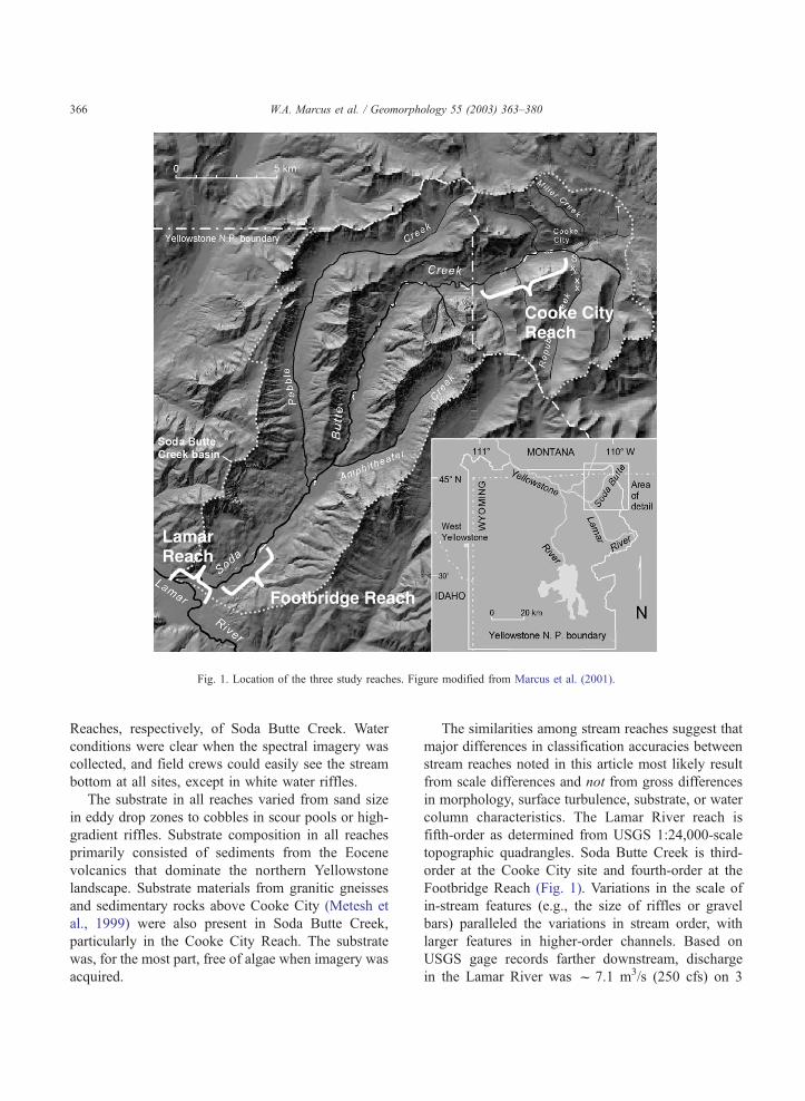
Fig. 1. Location of the three study reaches. Figure modified from Marcus et al. (2001).

W.A. Marcus et al. / Geomorphology 55 (2003) 363–380366

Reaches, respectively, of Soda Butte Creek. Water

conditions were clear when the spectral imagery was

collected, and field crews could easily see the stream

bottom at all sites, except in white water riffles.

The substrate in all reaches varied from sand size

in eddy drop zones to cobbles in scour pools or high-

gradient riffles. Substrate composition in all reaches

primarily consisted of sediments from the Eocene

volcanics that dominate the northern Yellowstone

landscape. Substrate materials from granitic gneisses

and sedimentary rocks above Cooke City (Metesh et

al., 1999) were also present in Soda Butte Creek,

particularly in the Cooke City Reach. The substrate

was, for the most part, free of algae when imagery was

acquired.

The similarities among stream reaches suggest that

major differences in classification accuracies between

stream reaches noted in this article most likely result

from scale differences and not from gross differences

in morphology, surface turbulence, substrate, or water

column characteristics. The Lamar River reach is

fifth-order as determined from USGS 1:24,000-scale

topographic quadrangles. Soda Butte Creek is third-

order at the Cooke City site and fourth-order at the

Footbridge Reach (Fig. 1). Variations in the scale of

in-stream features (e.g., the size of riffles or gravel

bars) paralleled the variations in stream order, with

larger features in higher-order channels. Based on

USGS gage records farther downstream, discharge

in the Lamar River was f 7.1 m3/s (250 cfs) on 3

W.A. Marcus et al. / Geomorphology 55 (2003) 363–380 367

August 1999 when imagery was collected. Discharge

at a USGS gage on the Footbridge Reach of Soda

Butte Creek was 3.9 m3/s (139 cfs) on 2 August 1999

when imagery was collected. Based on a ratio of

discharge to basin area, the discharge at the head of

the Cooke City Reach would have been 20% of that at

the Footbridge Reach, or f 0.79 m3/s (28 cfs).

4. Methods

4.1. Data collection

Hyperspectral data were collected on 3 August

1999 for the Lamar River and the Cooke City Reach

of Soda Butte Creek, and on 2 August 1999 for the

Footbridge Reach of Soda Butte Creek. Imagery was

collected using a Probe-1 sensor mounted on an A-

Star Aerospatiale helicopter flying 600 m above the

ground surface. The Probe-1 measured reflected

energy across 128 contiguous bands covering the

visible to shortwave–infrared portions of the spec-

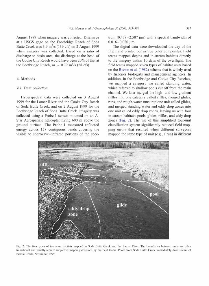
Fig. 2. The four types of in-stream habitats mapped in Soda Butte Cre

transitional and usually require subjective mapping decisions by the field

Pebble Creek, November 1999.

trum (0.438–2.507 Am) with a spectral bandwidth of

0.016–0.020 Am.

The digital data were downloaded the day of the

flight and printed out as true color composites. Field

teams mapped depths and in-stream habitats directly

to the imagery within 10 days of the overflight. The

field teams mapped seven types of habitat units based

on the Bisson et al. (1982) scheme that is widely used

by fisheries biologists and management agencies. In

addition, in the Footbridge and Cooke City Reaches,

we mapped a category we called standing water,

which referred to shallow pools cut off from the main

channel. We later merged the high- and low-gradient

riffles into one category called riffles, merged glides,

runs, and rough-water runs into one unit called glides,

and merged standing water and eddy drop zones into

one unit called eddy drop zones, leaving us with four

in-stream habitats: pools, glides, riffles, and eddy drop

zones (Fig. 2). The use of this simplified four-unit

classification system significantly reduced field map-

ping errors that resulted when different surveyors

mapped the same type of unit (e.g., a run) in different

ek and the Lamar River. The boundaries between units are often

teams. Photo from Soda Butte Creek immediately downstream of

W.A. Marcus et al. / Geomorphology 55 (2003) 363–380368

ways (e.g., as a run or as a glide or as a rough-water

run) (Marcus, 2002). Removing these disagreements

in field mapping was critical because such inconsis-

tency would have confused subsequent accuracy

assessments of image-based maps and made it diffi-

cult to determine whether classification errors indi-

cated limitations of the imagery or subjectivity in the

ground ‘‘truth’’ maps produced by field teams. More

detailed descriptions of these unit types are provided

in Ladd et al. (1998), Wright et al. (2000), Marcus et

al. (2002), and Legleiter et al. (2002).

Depths were mapped at points that could be clearly

located on both the image printouts and in the field.

We attempted to measure at least one depth in each

individual habitat unit (e.g., one point in every pool in

a given reach). Depths were measured using a ski pole

calibrated in 5-cm increments.

Woody debris in the Lamar River was mapped on

10–12 November 1999. Time and logistical con-

straints prevented field mapping of wood in other

reaches. No flows that were capable of moving the

wood occurred between the time of image acquisition

and field mapping. Wood was mapped directly to true

color printouts of the images to ensure precise cor-

egistration of imagery and maps. We only mapped

those pieces of wood longer than 2 m, >10 cm in

diameter, and clearly visible on the imagery.

4.2. Data analysis

All remote sensing analysis was conducted in

Environment for Visualizing Images (ENVI), a

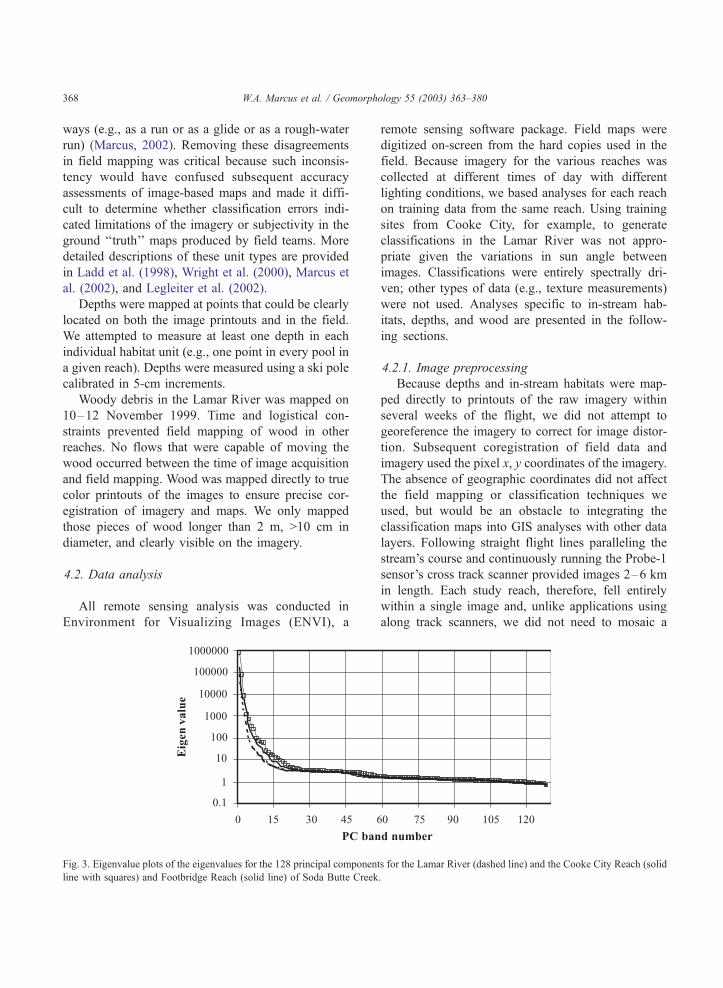
Fig. 3. Eigenvalue plots of the eigenvalues for the 128 principal componen

line with squares) and Footbridge Reach (solid line) of Soda Butte Creek

remote sensing software package. Field maps were

digitized on-screen from the hard copies used in the

field. Because imagery for the various reaches was

collected at different times of day with different

lighting conditions, we based analyses for each reach

on training data from the same reach. Using training

sites from Cooke City, for example, to generate

classifications in the Lamar River was not appro-

priate given the variations in sun angle between

images. Classifications were entirely spectrally dri-

ven; other types of data (e.g., texture measurements)

were not used. Analyses specific to in-stream hab-

itats, depths, and wood are presented in the follow-

ing sections.

4.2.1. Image preprocessing

Because depths and in-stream habitats were map-

ped directly to printouts of the raw imagery within

several weeks of the flight, we did not attempt to

georeference the imagery to correct for image distor-

tion. Subsequent coregistration of field data and

imagery used the pixel x, y coordinates of the imagery.

The absence of geographic coordinates did not affect

the field mapping or classification techniques we

used, but would be an obstacle to integrating the

classification maps into GIS analyses with other data

layers. Following straight flight lines paralleling the

stream’s course and continuously running the Probe-1

sensor’s cross track scanner provided images 2–6 km

in length. Each study reach, therefore, fell entirely

within a single image and, unlike applications using

along track scanners, we did not need to mosaic a

ts for the Lamar River (dashed line) and the Cooke City Reach (solid

.

Fig. 4. A schematic diagram of the general relation of morphologic

units to substrate size and surface turbulence of the water.

Table 1

Error matrix for maximum likelihood supervised classifications of

in-stream habitats using principal component images derived from

128-band hyperspectral imagerya

Image Ground truth (number of pixels)

classificationGlides Riffles Pools Eddy drop

zones

Total

Third-order, Cooke City Reach

Glides 2574 424 51 7 3056

Riffles 496 550 115 21 1182

Pools 191 30 95 2 318

Eddy drop zones 161 56 19 62 298

Total 3422 1060 280 92 4854

Fourth-order, Footbridge Reach

Glides 6152 561 25 10 6748

Riffles 2020 1047 11 0 3078

Pools 151 16 94 0 261

Eddy drop zones 7 0 0 22 29

Total 8330 1624 130 32 10,116

Fifth-order Lamar River Reach

Glides 6083 389 12 77 6561

Riffles 174 2653 6 23 2856

Pools 323 313 132 1 769

Eddy drop zones 139 142 2 564 847

Total 6719 3497 152 665 11,033

a A two-pixel (f2 m) spatial buffer has been removed from the

perimeter of each unit prior to accuracy assessment. Columns show

the number of pixels in a given class as mapped by the field team,

and the rows show the number of pixels in a given unit as classified

by the image. For example, 3422 total pixels were field mapped as

glides, of which 2572 were classified as glides on the image, 496 as

riffles, 191 as pools, and 161 as eddy drop zones. Data for the

Lamar River from Marcus (2002). Bolded values indicate number of

pixels correctly classified in each category.

W.A. Marcus et al. / Geomorphology 55 (2003) 363–380 369

number of separate scenes. The data were not atmos-

pherically corrected.

4.2.2. In-stream habitats

Field crews mapped in-stream habitats as polygons

that covered the entire stream. This article reports on

the results for classifying all the stream pixels that were

mapped as well as a spatially buffered version of the

original field map polygons. Spatial buffers were

applied because most boundaries between units were

fuzzy, with one unit (e.g., a riffle) gradually transition-

ing into the next (e.g., a glide) over a distance of several

meters. Removing a buffer zone where these transitions

occurred better represented the reality of the stream

environment.

Generating image-based classifications required

several steps. All nonstream areas were first masked

out. We then transformed the image data using a

nonstandardized, principal component algorithm to

minimize spectral noise and to reduce the number of

bands required for classification, a standard technique

in hyperspectral analysis. We used variance-based

PCA images rather than correlation-based PCA

because the variance-based images generated higher

classification accuracies. Classifications for each

reach were conducted using a maximum likelihood

supervised classification based on training sites from

the same reach. This maximum likelihood principal

component approach generated the best results among

the numerous techniques we investigated and is,

therefore, the focus of this article.

The classification was developed using 129 ran-

domly chosen training sites from each feature type in

each reach. The minimum number of training sites

required for a maximum likelihood supervised classi-

fication was 129 with 128 spectral bands as input

(Richards, 1994).

Eigenvalue plots (Fig. 3) indicated that over 100 of

the 128 principal components contributed significant

information (i.e., eigenvalue >1.0), but the highest

overall classification accuracies and kappa coeffi-

cients were generated using only the first 25 PC bands

in the Lamar River, the first 20 in the Cooke City

Reach, and the first 15 in the Footbridge Reach.

Classification accuracies gradually decreased as addi-

tional PC bands beyond this optimal number were

used for the classification (Marcus, 2002), presumably

because these additional bands included increasing

amounts of residual noise from the original images.

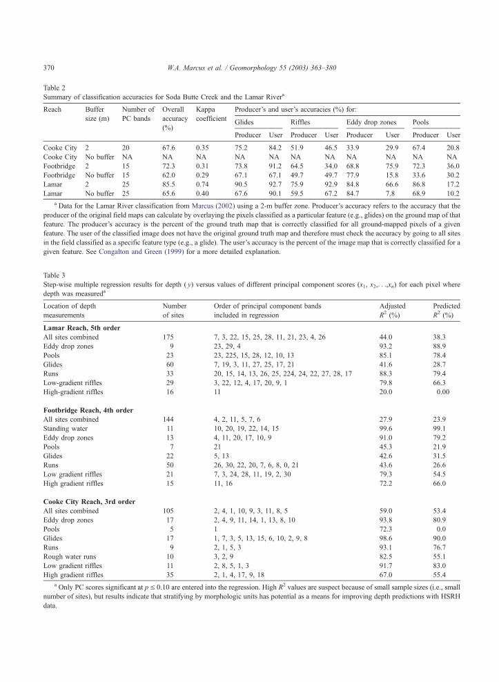
Table 2

Summary of classification accuracies for Soda Butte Creek and the Lamar Rivera

Reach Buffer Number of Overall Kappa Producer’s and user’s accuracies (%) for:

size (m) PC bands accuracy coefficientGlides Riffles Eddy drop zones Pools

(%)Producer User Producer User Producer User Producer User

Cooke City 2 20 67.6 0.35 75.2 84.2 51.9 46.5 33.9 29.9 67.4 20.8

Cooke City No buffer NA NA NA NA NA NA NA NA NA NA NA

Footbridge 2 15 72.3 0.31 73.8 91.2 64.5 34.0 68.8 75.9 72.3 36.0

Footbridge No buffer 15 62.0 0.29 67.1 67.1 49.7 49.7 77.9 15.8 33.6 30.2

Lamar 2 25 85.5 0.74 90.5 92.7 75.9 92.9 84.8 66.6 86.8 17.2

Lamar No buffer 25 65.6 0.40 67.6 90.1 59.5 67.2 84.7 7.8 68.9 10.2

a Data for the Lamar River classification from Marcus (2002) using a 2-m buffer zone. Producer’s accuracy refers to the accuracy that the

producer of the original field maps can calculate by overlaying the pixels classified as a particular feature (e.g., glides) on the ground map of that

feature. The producer’s accuracy is the percent of the ground truth map that is correctly classified for all ground-mapped pixels of a given

feature. The user of the classified image does not have the original ground truth map and therefore must check the accuracy by going to all sites

in the field classified as a specific feature type (e.g., a glide). The user’s accuracy is the percent of the image map that is correctly classified for a

given feature. See Congalton and Green (1999) for a more detailed explanation.

Table 3

Step-wise multiple regression results for depth ( y) versus values of different principal component scores (x1, x2,. . .,xn) for each pixel where

depth was measureda

Location of depth

measurements

Number

of sites

Order of principal component bands

included in regression

Adjusted

R2 (%)

Predicted

R2 (%)

Lamar Reach, 5th order

All sites combined 175 7, 3, 22, 15, 25, 28, 11, 21, 23, 4, 26 44.0 38.3

Eddy drop zones 9 23, 29, 4 93.2 88.9

Pools 23 23, 225, 15, 28, 12, 10, 13 85.1 78.4

Glides 60 7, 19, 3, 11, 27, 25, 17, 21 41.6 28.7

Runs 33 20, 15, 14, 13, 26, 25, 224, 24, 22, 27, 28, 17 88.3 79.4

Low-gradient riffles 29 3, 22, 12, 4, 17, 20, 9, 1 79.8 66.3

High-gradient riffles 16 11 20.0 0.00

Footbridge Reach, 4th order

All sites combined 144 4, 2, 11, 5, 7, 6 27.9 23.9

Standing water 11 10, 20, 19, 22, 14, 15 99.6 99.1

Eddy drop zones 13 4, 11, 20, 17, 10, 9 91.0 79.2

Pools 7 21 45.3 21.9

Glides 22 5, 13 42.6 31.5

Runs 50 26, 30, 22, 20, 7, 6, 8, 0, 21 43.6 26.6

Low gradient riffles 21 7, 3, 24, 28, 11, 19, 2, 30 79.3 54.5

High gradient riffles 15 11, 16 72.2 66.0

Cooke City Reach, 3rd order

All sites combined 105 2, 4, 1, 10, 9, 3, 11, 8, 5 59.0 53.4

Eddy drop zones 17 2, 4, 9, 11, 14, 1, 13, 8, 10 93.8 80.9

Pools 5 1 72.3 0.0

Glides 17 1, 7, 3, 5, 13, 15, 6, 10, 2, 9, 8 98.6 90.0

Runs 9 2, 1, 5, 3 93.1 76.7

Rough water runs 10 3, 2, 9 82.5 55.1

Low gradient riffles 11 2, 8, 5, 1, 3 91.7 83.0

High gradient riffles 35 2, 1, 4, 17, 9, 18 67.0 55.4

a Only PC scores significant at pV 0.10 are entered into the regression. High R2 values are suspect because of small sample sizes (i.e., small

number of sites), but results indicate that stratifying by morphologic units has potential as a means for improving depth predictions with HSRH

data.

W.A. Marcus et al. / Geomorphology 55 (2003) 363–380370

W.A. Marcus et al. / Geomorphology 55 (2003) 363–380 371

Classification accuracies reported in this article rep-

resent the maximum accuracies achieved when the

optimal number of PC bands were used.

Accuracy assessment followed standard confusion

matrix procedures, as outlined by Congalton and

Green (1999). Pixels used in the training set were

not used for evaluating classification accuracy.

4.2.3. Depth analysis

Depth analysis was conducted on the same princi-

pal component images used for the in-stream habitat

analysis. All depth sites within each reach were

entered into a stepwise multiple regression to deter-

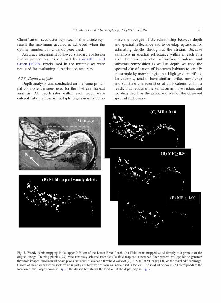
Fig. 5. Woody debris mapping in the upper 0.75 km of the Lamar River

original image. Training pixels (129) were randomly selected from the (

threshold images. Shown in white are pixels that equal or exceed a threshold

Choice of the appropriate threshold value is partly a subjective decision, as

location of the image shown in Fig. 6; the dashed box shows the location

mine the strength of the relationship between depth

and spectral reflectance and to develop equations for

estimating depths throughout the stream. Because

variations in spectral reflectance within a reach at a

given time are a function of surface turbulence and

substrate composition as well as depth, we used the

spectral classification of in-stream habitats to stratify

the sample by morphologic unit. High-gradient riffles,

for example, tend to have similar surface turbulence

and substrate characteristics at all locations within a

reach, thus reducing the variation in those factors and

isolating depth as the primary driver of the observed

spectral reflectance.

Reach. (A) Field teams mapped wood directly to a printout of the

B) field map and a matched filter process was applied to generate

value of (C) 0.18, (D) 0.50, or (E) 1.00 on the matched filter image.

is discussed in the text. The solid white box in (A) corresponds to the

of the depth map in Fig. 7.

W.A. Marcus et al. / Geomorphology 55 (2003) 363–380372

For purposes of depth analysis, we used the orig-

inal eight in-stream habitats (high- and low-gradient

riffles, eddy drop zones, standing water, rough-water

runs, runs, glides, and pool) rather than merging the

units into riffles, glides, pools, and eddy drop zones as

was done for the mapping of in-stream units. Use of

the eight units better stratified the stream by surface

turbulence and substrate size, although some overlap

between units was present (Fig. 4). Stratifying the

sample using the image-based classification of in-

stream units rather than our field maps provided a

better indication of the potential of the technique to be

applied in areas where field teams are not available to

generate detailed ground maps prior to using the

imagery for depth analysis.

4.2.4. Wood analysis

Procedures for classifying wood initially followed

the same techniques used for in-stream habitats. A

mask was used to remove features outside the exposed

bars where wood was located. We then performed a

principal component transformation on the remaining

portion of the image.

We used the matched filter (MF) approach in ENVI

to identify woody debris in the principal component

image. The MF algorithm performs a partial unmixing

of spectra to estimate the relative quantity of a given

material in a pixel based on user-defined spectral end

members (wood in this case) (Harsanyi and Chang,

1994; Boardman et al., 1995). Matched filtering has

the advantage of not requiring knowledge of all end

members within an image scene and so can be used to

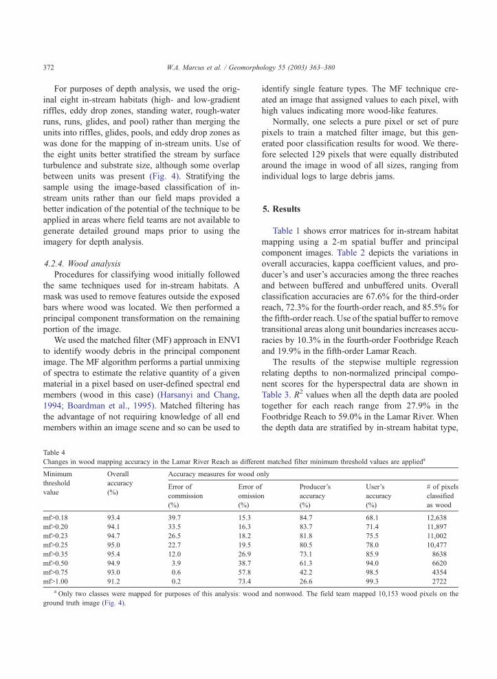
Table 4

Changes in wood mapping accuracy in the Lamar River Reach as differe

Minimum Overall Accuracy measures for wood o

threshold

value

accuracy

(%)Error of

commission

(%)

Error o

omissio

(%)

mf>0.18 93.4 39.7 15.3

mf>0.20 94.1 33.5 16.3

mf>0.23 94.7 26.5 18.2

mf>0.25 95.0 22.7 19.5

mf>0.35 95.4 12.0 26.9

mf>0.50 94.9 3.9 38.7

mf>0.75 93.0 0.6 57.8

mf>1.00 91.2 0.2 73.4

a Only two classes were mapped for purposes of this analysis: wood

ground truth image (Fig. 4).

identify single feature types. The MF technique cre-

ated an image that assigned values to each pixel, with

high values indicating more wood-like features.

Normally, one selects a pure pixel or set of pure

pixels to train a matched filter image, but this gen-

erated poor classification results for wood. We there-

fore selected 129 pixels that were equally distributed

around the image in wood of all sizes, ranging from

individual logs to large debris jams.

5. Results

Table 1 shows error matrices for in-stream habitat

mapping using a 2-m spatial buffer and principal

component images. Table 2 depicts the variations in

overall accuracies, kappa coefficient values, and pro-

ducer’s and user’s accuracies among the three reaches

and between buffered and unbuffered units. Overall

classification accuracies are 67.6% for the third-order

reach, 72.3% for the fourth-order reach, and 85.5% for

the fifth-order reach. Use of the spatial buffer to remove

transitional areas along unit boundaries increases accu-

racies by 10.3% in the fourth-order Footbridge Reach

and 19.9% in the fifth-order Lamar Reach.

The results of the stepwise multiple regression

relating depths to non-normalized principal compo-

nent scores for the hyperspectral data are shown in

Table 3. R2 values when all the depth data are pooled

together for each reach range from 27.9% in the

Footbridge Reach to 59.0% in the Lamar River. When

the depth data are stratified by in-stream habitat type,

nt matched filter minimum threshold values are applieda

nly

f

n

Producer’s

accuracy

(%)

User’s

accuracy

(%)

# of pixels

classified

as wood

84.7 68.1 12,638

83.7 71.4 11,897

81.8 75.5 11,002

80.5 78.0 10,477

73.1 85.9 8638

61.3 94.0 6620

42.2 98.5 4354

26.6 99.3 2722

and nonwood. The field team mapped 10,153 wood pixels on the

W.A. Marcus et al. / Geomorphology 55 (2003) 363–380 373

adjusted R2 values vary widely, ranging from 20.0%

for high-gradient riffles in the Cooke City Reach to

99.6% for standing water in the Footbridge Reach.

Fig. 5 portrays a black-and-white composite image

of the area where wood was mapped, the field map of

wood, and wood classifications based on matched

filter analysis using different minimum thresholds.

Table 4 shows the changes in different accuracy

measures that occur as different threshold values are

used. The implications of using different thresholds

are discussed below.

6. Discussion

The following sections on in-stream habitats,

depth, and woody debris discuss issues specific to

each parameter. We also describe factors affecting

mapping accuracy, possibilities for improving classi-

fication results, extensions of HSRH mapping to

watershed scales, and future research directions. The

section concludes with some general comments that

apply to HSRH mapping of these three important

stream parameters.

6.1. In-stream habitats

The ability of HSRH imagery to classify in-stream

habitats varied with stream scale. Overall and produc-

er’s accuracies consistently improved as stream order

increased (Table 2). The greater accuracy in the fifth-

order Lamar River probably occurred because larger

streams feature more sizable, more homogenous units

than do smaller streams. This, in turn, significantly

reduced the proportion of the stream occupied by

transitional boundary areas between in-stream habitats

as well as the amount of internal variability displayed

within a single unit (e.g., small riffle-like areas within

a glide).

The application of the 2-m buffer improved clas-

sification accuracies (Table 2) by removing a portion

of the transitional boundary zone that is difficult to

map in the field. Even with the 2-m buffer, however,

image-based classifications often displayed a mix of

unit types on the margins of individual units. These

regions generated apparent classification errors when

compared to the homogenous ground-truth polygons

mapped by field teams.

One approach to resolving the discrepancies

between homogenous ground truth maps and hetero-

geneous classifications would be to use post-classi-

fication filters that ‘‘clump and sieve’’ the classified

pixels to create more cohesive classification units.

This post-classification fix would ignore, however,

the possibility that the concentration of pixel-scale

heterogeneity at unit boundaries on the image maps is

real; i.e., that the imagery may provide more accurate

and precise maps than the ground teams (Marcus,

2002; Legleiter et al., 2002). For example, close

examination of Fig. 6 shows a scattering of riffle

and glide pixels near unit boundaries, suggesting that

the imagery detected subtle variations where surface

roughness is locally riffle-like, but glide-like only a

few centimeters away. Such variations are indeed

observed in the field, but ground teams could not

map at this scale because of time limitations and the

difficulty of precisely locating the pixel on the image.

The field team’s placement of unit boundaries through

these transitional areas was also somewhat arbitrary.

The image classification also indicates shoreline

boundary effects that make sense from a hydraulic

perspective. Areas mapped as riffles by the field team

are shown by the imagery to have glide pixels near the

shoreline; a feature that occurs as water shallows and

slows at stream edges (Fig. 6). Eddy drop zones are

shown immediately adjacent to the shore, where water

velocity drops to nearly zero and sands and silts are

deposited along the banks. These features, however,

were too small to be mapped in the field.

Two primary sources of ground survey error there-

fore probably led to discrepancies between field maps

and image-based maps: (i) inconsistent identification

of units by field crews; and (ii) lumping of small

regions of variability (e.g., a small riffle) into a larger

more homogenous region (e.g., a glide). Based on this

rationale and on our experience with the field sites, we

believe that the HSRH maps were more consistent and

precise in their characterization of unit boundaries and

heterogeneity than the large, homogenous polygons

created by the field teams. If this is the case, then the

poorer classification results in the Cooke City Reach

may not reflect a weakness of the classification capa-

bilities of HSRH imagery in lower-order streams, but

a weakness of the techniques used to field map and

validate the image classifications in these tremendous-

ly variable environments.

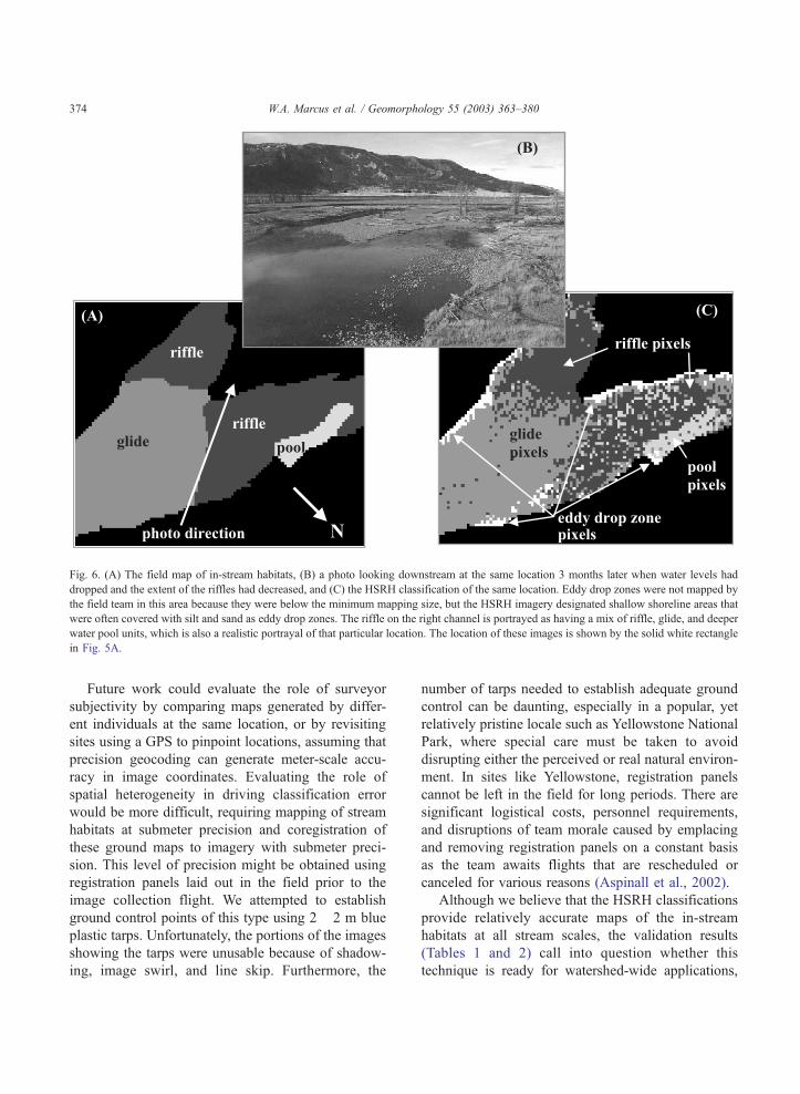
Fig. 6. (A) The field map of in-stream habitats, (B) a photo looking downstream at the same location 3 months later when water levels had

dropped and the extent of the riffles had decreased, and (C) the HSRH classification of the same location. Eddy drop zones were not mapped by

the field team in this area because they were below the minimum mapping size, but the HSRH imagery designated shallow shoreline areas that

were often covered with silt and sand as eddy drop zones. The riffle on the right channel is portrayed as having a mix of riffle, glide, and deeper

water pool units, which is also a realistic portrayal of that particular location. The location of these images is shown by the solid white rectangle

in Fig. 5A.

W.A. Marcus et al. / Geomorphology 55 (2003) 363–380374

Future work could evaluate the role of surveyor

subjectivity by comparing maps generated by differ-

ent individuals at the same location, or by revisiting

sites using a GPS to pinpoint locations, assuming that

precision geocoding can generate meter-scale accu-

racy in image coordinates. Evaluating the role of

spatial heterogeneity in driving classification error

would be more difficult, requiring mapping of stream

habitats at submeter precision and coregistration of

these ground maps to imagery with submeter preci-

sion. This level of precision might be obtained using

registration panels laid out in the field prior to the

image collection flight. We attempted to establish

ground control points of this type using 2� 2 m blue

plastic tarps. Unfortunately, the portions of the images

showing the tarps were unusable because of shadow-

ing, image swirl, and line skip. Furthermore, the

number of tarps needed to establish adequate ground

control can be daunting, especially in a popular, yet

relatively pristine locale such as Yellowstone National

Park, where special care must be taken to avoid

disrupting either the perceived or real natural environ-

ment. In sites like Yellowstone, registration panels

cannot be left in the field for long periods. There are

significant logistical costs, personnel requirements,

and disruptions of team morale caused by emplacing

and removing registration panels on a constant basis

as the team awaits flights that are rescheduled or

canceled for various reasons (Aspinall et al., 2002).

Although we believe that the HSRH classifications

provide relatively accurate maps of the in-stream

habitats at all stream scales, the validation results

(Tables 1 and 2) call into question whether this

technique is ready for watershed-wide applications,

W.A. Marcus et al. / Geomorphology 55 (2003) 363–380 375

especially in smaller streams. In particular, although

the producer’s accuracies for the 2-m buffered units

typically approached or exceeded the 85% criteria

often considered acceptable for remote sensing clas-

sifications, the user’s accuracies were often notably

lower, especially for the smaller units (pools and eddy

drop zones) that make up a small portion of the total

stream area (Table 2). Unfortunately, these small pool

and eddy drop zone units are often most important as

fish habitat and sites of contaminated sediment accu-

mulation (Ladd et al., 1998), making these the fea-

tures managers are most interested in mapping.

A number of options are available for improving

the classification accuracies at all scales. Scaling the

size of the spatial buffer to the stream size, for

example, could remove more of the confusion caused

by transitional zones between units. For example, one

might apply a 4-m buffer in the Lamar, a 3-m buffer in

the Footbridge Reach, and a 2-m buffer in the Cooke

City Reach. This has the disadvantage, however, of

not classifying increasingly larger areas of the river as

stream size grows. Developing clearer criteria for field

mapping boundaries of habitat units might also

improve accuracies by ensuring consistency amongst

field maps and subsequent selection of training sites

for image classification. Fuzzy classifications (e.g.,

Wright et al., 2000) may be particularly appropriate

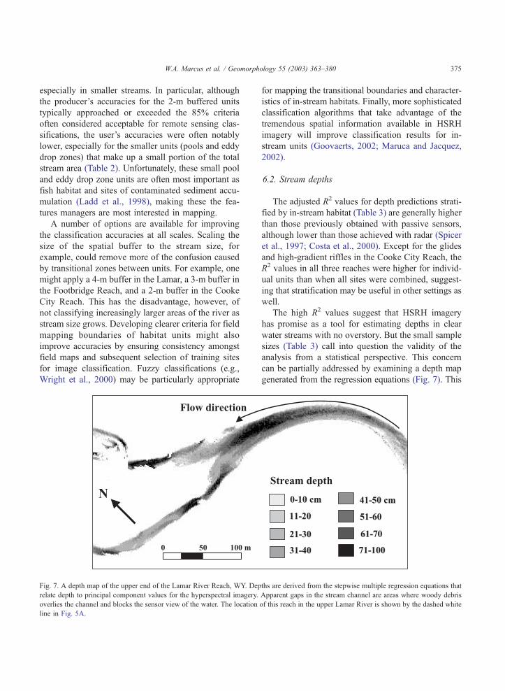
Fig. 7. A depth map of the upper end of the Lamar River Reach, WY. Dep

relate depth to principal component values for the hyperspectral imagery.

overlies the channel and blocks the sensor view of the water. The location

line in Fig. 5A.

for mapping the transitional boundaries and character-

istics of in-stream habitats. Finally, more sophisticated

classification algorithms that take advantage of the

tremendous spatial information available in HSRH

imagery will improve classification results for in-

stream units (Goovaerts, 2002; Maruca and Jacquez,

2002).

6.2. Stream depths

The adjusted R2 values for depth predictions strati-

fied by in-stream habitat (Table 3) are generally higher

than those previously obtained with passive sensors,

although lower than those achieved with radar (Spicer

et al., 1997; Costa et al., 2000). Except for the glides

and high-gradient riffles in the Cooke City Reach, the

R2 values in all three reaches were higher for individ-

ual units than when all sites were combined, suggest-

ing that stratification may be useful in other settings as

well.

The high R2 values suggest that HSRH imagery

has promise as a tool for estimating depths in clear

water streams with no overstory. But the small sample

sizes (Table 3) call into question the validity of the

analysis from a statistical perspective. This concern

can be partially addressed by examining a depth map

generated from the regression equations (Fig. 7). This

ths are derived from the stepwise multiple regression equations that

Apparent gaps in the stream channel are areas where woody debris

of this reach in the upper Lamar River is shown by the dashed white

W.A. Marcus et al. / Geomorphology 55 (2003) 363–380376

map is hydraulically reasonable, with depths that are

consistently deepest in the thalweg, cut banks of

meander bends, or areas of flow convergence and

channel scour. Likewise, the map shows shallow

depths along the inside of bends and in areas of flow

divergence. Depth ranges displayed by the map are in

close agreement with those that occurred in the

stream.

The accuracy of depth estimates did not vary in a

consistent manner between the stream reaches,

although the poorest R2 values all occurred in the

lower-order streams. The lower values in smaller

streams may have been driven by the relative increase

in the number of mixed pixels, where a wide range of

depths and surface turbulence occurred within a single

pixel. Stream size will put a bounding limit on the

ability of this depth detection technique to work

because it cannot be applied in streams that are small

enough for banks or overstory to block the sensor’s

view of the water.

The greatest influence on the accuracy of the

technique appears to be surface turbulence, with

greater surface turbulence interfering with the sen-

sor’s ability to penetrate the water and provide ac-

curate depth estimates. For the most part, units with

little surface turbulence (pools, eddy drop zones, and

standing water) displayed higher R2 values. R2 values

for other units did not vary in a consistent fashion,

although high-gradient riffles (the most turbulent of

the units) had the lowest R2 values in the Cooke City

and Lamar Reaches.

The principal component scores most strongly

correlated with depth (i.e., the first scores entered into

the stepwise regression) did not follow the rank order

of the principal components. Apparently, the signal

related to depth is captured within subtle variations in

the spectral reflectance of the water. Combined with

the large number of principal component scores

required to achieve high R2 values, this emphasizes

the desirability of hyperspectral rather than multi-

spectral imagery. In addition, HSRH imagery is nec-

essary to accurately classify the in-stream habitats

(Marcus, 2002; Legleiter et al., 2002), a key step in

stratifying the stream data in order to improve accu-

racy.

Finally, the creation of continuous depth maps like

Fig. 7 raises the exciting possibility of creating con-

tinuous maps for shear stress and stream power. This

could be accomplished by coregistering depth maps

with high-resolution DEM-based maps of bed slope

or, alternatively, by measuring water surface slopes

from radar or lidar imagery. Such maps developed at

watershed scales would be remarkably valuable tools

for understanding stream habitats and disturbance

impacts, predicting channel change, and providing

the empirical data needed to create and evaluate

thermodynamic theories about the distribution of

energy expenditure in fluvial systems.

6.3. Woody debris

The data in Fig. 5 and Table 4 indicate that wood

can be readily identified on hyperspectral imagery.

When evaluating a two-class system (wood and

nonwood in this case), no single-matched filter

threshold value provided the ‘‘best’’ accuracy. Data

from Table 4 suggest, for example, that 1.0 would be

the best threshold value for minimizing errors of

commission, which occur when nonwood areas are

classified as wood. A value of 1.0, however, max-

imizes the errors of omission, which occur when

wood pixels are classified as nonwood. Similar

arguments can be made for producer’s and user’s

accuracy, where choosing a high threshold value of

1.0 ensures that almost every image map pixel

visited by a user will be wood, but also misses

many of the wood pixels mapped by field teams

(i.e., the producers of the data). The choice of a

threshold will ultimately depend on the map maker’s

and map user’s willingness to accept certain types of

error.

We believe that wood, because of its strong spec-

tral signature, can be detected even when it covers

only a portion of a pixel. For example, a pixel with a

matched filter threshold value of 0.75 and above

might represent a pixel covered entirely by wood,

while a value >0.18 but < 0.25 might represent a pixel

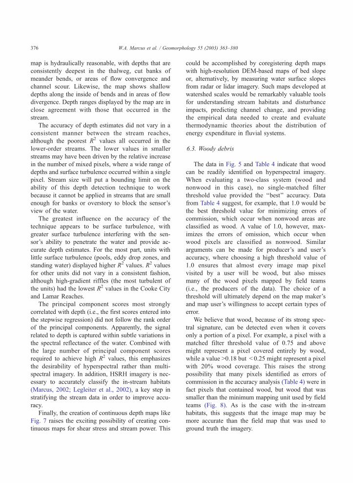
with 20% wood coverage. This raises the strong

possibility that many pixels identified as errors of

commission in the accuracy analysis (Table 4) were in

fact pixels that contained wood, but wood that was

smaller than the minimum mapping unit used by field

teams (Fig. 8). As is the case with the in-stream

habitats, this suggests that the image map may be

more accurate than the field map that was used to

ground truth the imagery.

Fig. 8. Wood in the Lamar River Reach that was smaller than the

minimum size (2 m long and 10-cm diameter) mapped by field

teams. Even though wood of this size was not mapped by field

teams, it was probably sensed by the hyperspectral imagery and

shows up on matched filter maps (Fig. 5), creating false errors of

commission in the accuracy analysis. The footprint of a hypothetical

1-m pixel is shown in white.

W.A. Marcus et al. / Geomorphology 55 (2003) 363–380 377

The results depicted in Fig. 5 and Table 4 indicate

that hyperspectral imagery has great potential as a tool

for mapping woody debris, especially at watershed

scales where the personnel, cost, and time required for

ground mapping can be prohibitive. The only signifi-

cant logistical obstacles to image-based mapping of

wood occur when wood is obstructed by water,

vegetation, or shadows.

Several issues should be addressed, however, to

improve validation procedures and classification ac-

curacies. The greatest difficulties we encountered re-

sulted from line skip, line oversampling, and image

swirl created by platform motion, all of which com-

bined to make it impossible to accurately georeference

the image (Aspinall et al., 2002). This concern was

partially bypassed by only mapping wood that could

be clearly identified on printouts of the imagery. This

approach, however, did not permit field mapping of

wood smaller than what could be seen on the imagery,

which in turn limited the effectiveness of accuracy

assessment techniques. In particular, we could not

match areas where subpixel wood coverage was

indicated by the matched filter image (e.g., Fig. 5C)

to corresponding ground sites (e.g., Fig. 8), because

the image and ground coordinates could not be

coregistered to pixel-scale resolution. Future wood

mapping should be done using high quality geo-

corrected imagery. Corrections at this precision can

be accomplished using ray tracing methods for post-

correction (Boardman, 1999).

The wood classification worked best when using

pixels scattered throughout the image as training sites,

rather than when using one or a small number of pure

pixels, which is the more standard approach with

matched filters. We speculate that the scattered pixel

approach worked better because (i) woody debris is

heterogeneous, with some that has bark, some that is

burned, some that has foliage, and so on; and (ii) the

1-m imagery was not corrected for bidirectional

reflectance, so that a series of points from across the

entire image captured the range of image spectra for

wood better than spectra from just one or two sites.

This suggests that segregating the wood by attribute

(with or without bark, burned or not burned, with or

without foliage, etc.) should improve wood detection

by providing purer spectral signatures on which to

train the matched filter. In addition, atmospheric

correction and removal of bidirectional reflectance

both might improve the detectability of wood.

6.4. General considerations

Regardless of the parameter being mapped, we

encountered a number of difficulties with image

acquisition and processing that are likely to plague

any research team using HSRH imagery (Aspinall et

al., 2002). Coordination of overflights with field

teams was remarkably difficult given the dependence

on weather, stream conditions, availability of hyper-

spectral sensors, and the large number of people that

must be mobilized to collect sufficient ground data in

a timely fashion. Accurate, pixel-scale georeferencing

W.A. Marcus et al. / Geomorphology 55 (2003) 363–380378

and coregistration of imagery and ground data were

not possible with submeter-scale precision. Finally,

bidirectional reflectance created particular problems

with high spatial resolution imagery because the

narrow swath width of the cross track scanner

(f 500 m at 1-m pixel resolution with the PROBE-

1 sensor) made it difficult to keep the streams near the

center of the flight line.

The difficulty in realistically evaluating the accu-

racy of pixel-scale variations shown on the imagery

for in-stream habitats and for subpixel variations in

wood indicates that alternative means for accuracy

assessment are needed. Accuracy assessment for both

wood and in-stream habitat mapping could benefit

from (i) pixel-scale ground mapping coupled with use

of techniques that provide pixel-scale accuracy in

coregistering images and field maps (e.g., Clark et

al., 1998; Boardman, 1999); and (ii) the development

of techniques that enable realistic comparisons

between the pixel- and subpixel-scale variations

shown on images and the field maps with their large,

homogenous polygons or one class per pixel portrayal

of the surface (Aspinall, 2002). Mapping of in-stream

habitats in particular will benefit from spatial models

that aggregate pixel-scale variations into larger nearby

units, thus generating an image classification that

more closely matches the homogenous polygons

mapped by field teams (e.g., Goovaerts, 2002; Maruca

and Jacquez, 2002).

The approach taken in this study was ‘‘top-down,’’

meaning that spectra from the airborne image were

used to drive the classification. These image spectra,

however, represent a mixture of all the factors affect-

ing the electromagnetic radiation as it travels from the

target to the sensor. The reflectance spectra for in-

stream habitats, for example, represent variations in

reflectance because of surface turbulence, substrate

size, substrate color and composition, periphyton,

turbidity, and depth, not to mention atmospheric

effects. The development of deterministic, ‘‘bottom-

up’’ models [such as that devised by Lyon and

Hutchinson (1995)] could be valuable for developing

classification schemes that can be applied across

multiple watersheds and multiple images without

requiring such extensive ground truth collection

efforts. These models would also provide an important

explanatory tool for understanding variations in spec-

tral signals in different settings.

Finally, visual examination of the spectral curves

and of unsupervised classifications for both Soda

Butte Creek and the Lamar River shows that the

hyperspectral sensor is capturing far more information

about the stream environment than can be conveyed in

a simple four-unit classification or a wood/nonwood

dichotomy. HSRH-driven unsupervised classifications

of the stream environment coupled with subsequent

ground investigations might well open our eyes to

critical components of the stream system that have

previously been overlooked.

7. Summary and conclusions

Overall classification accuracies for in-stream hab-

itats (glides, riffles, pools, and eddy drop zones)

ranged from 69% for third-order streams to 86%

for fifth-order streams (Table 2). R2 values for com-

parisons of measured and estimated depths ranged

from 20% for high-gradient riffles in third-order

reaches to 99% for glides in the fifth-order reach

(Table 3). The accuracy of woody debris mapping

covered a wide range, depending on the threshold

value chosen for the matched filter (Table 4). Visual

analysis of image-based maps of in-stream habitats

(Fig. 6), depths (Fig. 7), and wood (Fig. 5) all

suggests that HSRH imagery generated results that

are more accurate and useful than the validation

statistics alone seem to suggest.

Given clear water and an unobstructed view of the

stream, our results indicate that there is great potential

for HSRH mapping and monitoring of streams. In a

number of cases, accuracies approached or exceeded

the 85% value typically expected for remote sensing

mapping. The ability to remotely map and monitor

stream channels at spatial scales of 1 m raises exciting

prospects for the advancement of stream studies. In

particular, HSRH has the potential to enable exami-

nation of the pattern, process, and scale so critical to

understanding fluvial ecosystems (Walsh et al., 1998)

at resolutions previously thought to be obtainable only

with localized ground-based monitoring (Muller et al.,

1993).

Methodological hurdles remain to be overcome,

however, before we can be confident in HSRH-based

stream maps. In particular, relative to our study,

improved procedures should be used or developed

W.A. Marcus et al. / Geomorphology 55 (2003) 363–380 379

for georectifying images, removing bidirectional

reflectance, assessing accuracy (including the field

mapping component), and analyzing the tremendous

spatial as well as spectral information in HSRH

imagery. These methodological advances need to be

coupled with a greater understanding of the spectral

characteristics of streams in order to explain classi-

fication results and their variation among sites. Only if

these studies are undertaken and new working tools

developed will the full potential of HSRH mapping of

streams be realized.

Acknowledgements

This research was supported by the NASA EOCAP

program, Stennis Space Flight Center, Mississippi.

William Graham, Joseph Spruce, and Greg Terrie of

Stennis Space Flight Center all provided important

logistical support and technical advice. Robert Ahl,

Kerry Halligan, and Jim Rasmussen collected ground

truth data. The senior author wishes to thank Samuel

Goward for introducing him to the field of remote

sensing and supporting his early research efforts to

apply remote sensing technology to watershed

measurement and modeling.

References

Aspinall, R.J., 2002. Use of logistic regression for validation of

maps of the spatial distribution of vegetation derived from high

spatial resolution hyperspectral remotely sensed data. Ecological

Modelling. Special Issue on Advances in Generalized Linear/

Generalized Additive Modelling: from Species’ Distribution to

Environmental Management 157 (2–3), 301–312.

Aspinall, R., Marcus, W.A., Boardman, J.W., 2002. Considerations

in collecting, processing, and analysing high spatial resolution

hyperspectral data for environmental investigations. Journal of

Geographical Systems 4 (1), 15–29.

Bisson, P.A., Nielson, J.L., Palmalson, R.A., Grove, L.E., 1982.

A system of naming habitat types in small streams, with ex-

amples of habitat utilization by salmonids during low stream

flow. In: Armantrout, N.B. (Ed.), Acquisition and Utilization

of Aquatic Habitat Inventory Information. Proceedings Ame-

rican Fisheries Society, Portland, OR, pp. 62–73.

Boardman, J.W., 1989. Inversion of imaging spectrometry data

using singular value decomposition. Proceedings, IGARSS’89,

12th Canadian Symposium on Remote Sensing 4, 2069–2072.

Boardman, J.W., 1993. Automated spectral unmixing of AVIRIS data

using convex geometry concepts. Summaries, 4th Jet Propulsion

Laboratory Airborne Geoscience Workshop, Jet Propulsion Lab-

oratory Publication 93-26. 14 pp. http://popo.jpl.nasa.gov/docs/

workshops/93_docs/4.pdf.

Boardman, J.W., 1999. Precision geocoding of low altitude AVIRIS

data: lessons learned in 1998. AVIRIS 1999 Proceedings, Jet

Propulsion Laboratory, CA. 6 pp. http://makalu.jpl.nasa.gov/

docs/workshops/99_docs/7.pdf.

Boardman, J.W., Kruse, F.A., Green, R.O., 1995. Mapping target

signatures via partial unmixing of AVIRIS data. Summaries, Fifth

JPL Airborne Earth Science Workshop, Jet Propulsion Labora-

tory Publication 95-1, pp. 23–26. http://popo.jpl.nasa.gov/docs/

workshops/95_docs/7.pdf.

Clark, R.N., Livo, K.E., Kokaly, R.F., 1998. Geometric correction

of AVIRIS imagery using on-board navigation and engineering

data. AVIRIS 1998 Proceedings, Jet Propulsion Laboratory, CA.

9 pp. http://makalu.jpl.nasa.gov/docs/workshops/98_docs/9.pdf.

Congalton, R.G., Green, K., 1999. Assessing the Accuracy of Re-

motely Sensed Data: Principles and Practices. Lewis Publishers,

New York. 137 pp.

Costa, J.E., Spicer, K.R., Cheng, R.T., Haeni, F.P., Melcher, N.B.,

Thurman, M.E., Plant, W.J., Keller, W.C., 2000. Measuring

stream discharge by non-contact methods: a proof of concept

experiment. Geophysical Research Letters 27 (4), 553–556.

Gilvear, D.J., Waters, T.M., Milner, A.M., 1995. Image analysis of

aerial photography to quantify changes in channel morphology

and instream habitat following placer mining in interior Alaska.

Freshwater Biology 34, 389–398.

Goovaerts, P., 2002. Geostatistical incorporation of spatial coordi-

nates into supervised classification of hyperspectral data. Jour-

nal of Geographical Systems 4 (1), 99–111.

Hardy, T.B., Anderson, P.C., Neale, M.U., Stevens, D.K., 1994.

Application of multispectral videography for the delineation of

riverine depths and mesoscale hydraulic features. In: Marston,

R., Hasfurther, V. (Eds.), Effects of Human-Induced Change on

Hydrologic Systems. Proceedings Annual Water Resources As-

sociation, Jackson Hole, WY, pp. 445–454.

Harsanyi, J.C., Chang, C.I., 1994. Hyperspectral image classifica-

tion and dimensionality reduction: an orthogonal subspace pro-

jection approach. IEEE Transactions on Geoscience and Remote

Sensing 32, 779–785.

Ladd, S., Marcus, W.A., Cherry, S., 1998. Trace metal segregation

within morphologic units. Environmental Geology and Water

Sciences 36, 195–206.

Legleiter, C.J., Marcus, W.A., Lawrence, R., 2002. Effects of sensor

resolution on mapping in-stream habitats. Photogrammetric En-

gineering and Remote Sensing 68, 801–807.

Lyon, J.G., Hutchinson, W.S., 1995. Application of a radiometric

model for evaluation of water depths and verification of results

with airborne scanner data. Photogrammetric Engineering and

Remote Sensing 61, 161–166.

Lyon, J.G., Lunetta, R.S., Williams, D.C., 1992. Airborne multi-

spectral scanner data for evaluating bottom sediment types and

water depths of the St. Marys River, Michigan. Photogrammet-

ric Engineering and Remote Sensing 58, 951–956.

Marcus, W.A., 2002. Mapping of stream microhabitats with high

spatial resolution hyperspectral imagery. Journal of Geographi-

cal Systems 4 (1), 113–126.

W.A. Marcus et al. / Geomorphology 55 (2003) 363–380380

Marcus, W.A., Meyer, G.A., Nimmo, D.R., 2001. Geomorphic con-

trol on long-term persistence of mining impacts, Soda Butte

Creek, Yellowstone National Park. Geology 29, 355–358.

Marcus, W.A., Marston, R.A., Colvard Jr., C.R., Gray, R.D., 2002.

Mapping the spatial and temporal distributions of large woody

debris in rivers of the Greater Yellowstone Ecosystem. U.S.A.,

Geomorphology 44 (3–4), 323–335.

Maruca, S.L., Jacquez, G.M., 2002. Area-based tests for association

between spatial patterns. Journal of Geographical Systems 4 (1),

69–83.

Metesh, J., English, A., Lonn, J., Kendy, E., Parrett, C., 1999.

Hydrogeology of the upper Soda Butte Creek basin, Montana.

Montana Bureau of Mines and Geology Report of Investigation,

vol. 7. 66 pp.

Meyer, G.A., 2001. Recent large-magnitude floods and their impact

on valley-floor environments of northeastern Yellowstone. Geo-

morphology 40 (3–4), 271–290.

Minshall, G.W., Robinson, C.T., Robinson, T.V., Royer, T.V., 1998.

Stream ecosystem responses to the 1988 wildfires. Yellowstone

Science 6 (3), 15–22.

Montgomery, D.R., Buffington, J.M., 1997. Channel-reach mor-

phology in mountain drainage basins. Geological Society of

American Bulletin 109 (5), 596–611.

Muller, E., Decamps, H., Dobson, M.K., 1993. Contribution of

space remote sensing to river studies. Freshwater Biology 29,

301–312.

Orth, D.J., Maughan, O.E., 1983. Microhabitat preferences of

benthic fauna in a woodland stream. Hydrobiologica 106,

157–168.

Richards, J.A., 1994. Remote Sensing Digital Image Analysis.

Springer, Berlin. 340 pp.

Spicer, K.R., Costa, J.E., Placzek, G., 1997. Measuring flood dis-

charge in unstable stream channels using ground penetrating

radar. Geology 25 (5), 423–426.

Ustin, S.L., Costick, L., 2000. Multispectral remote sensing over

semi-arid landscapes for resource management. In: Hill, M.J.,

Aspinall, R.J. (Eds.), Spatial Information for Land Use Manage-

ment. Gordon and Breach, London, pp. 97–109. Chapter 8.

Walsh, S.J., Butler, D., Malanson, G.P., 1998. An overview of scale,

pattern, process relationships in geomorphology: a remote sens-

ing and GIS perspective. Geomorphology 21, 183–205.

Winterbottom, S.J., Gilvear, D.J., 1997. Quantification of channel-

bed morphology in gravel-bed rivers using airborne multispec-

tral imagery and aerial photography. Regulated Rivers: Research

and Management 13, 489–499.

Wright, A., Marcus, W.A., Aspinall, R.J., 2000. Applications and

limitations of using multispectral digital imagery to map geo-

morphic stream units in a lower order stream. Geomorphology

33 (1–2), 107–120.