
HIGH RESOLUTION DIRECTION OF ARRIVAL ESTIMATION …
192
HIGH RESOLUTION DIRECTION OF ARRIVAL ESTIMATION ANALYSIS AND IMPLEMENTATION IN A SMART ANTENNA SYSTEM by Ahmed Khallaayoun A dissertation submitted in partial fulfillment of the requirements for the degree of Doctor of Philosophy in Electrical Engineering MONTANA STATE UNIVERSITY Bozeman, Montana May, 2010
Transcript of HIGH RESOLUTION DIRECTION OF ARRIVAL ESTIMATION …

HIGH RESOLUTION DIRECTION OF ARRIVAL
ESTIMATION ANALYSIS AND IMPLEMENTATION IN
A SMART ANTENNA SYSTEM
by
Ahmed Khallaayoun
A dissertation submitted in partial fulfillmentof the requirements for the degree
of
Doctor of Philosophy
in
Electrical Engineering
MONTANA STATE UNIVERSITYBozeman, Montana
May, 2010

©COPYRIGHT
by
Ahmed Khallaayoun
2010
All Rights Reserved

ii
APPROVAL
of a dissertation submitted by
Ahmed Khallaayoun
This dissertation has been read by each member of the dissertation committee andhas been found to be satisfactory regarding content, English usage, format, citation,bibliographic style, and consistency and is ready for submission to the Division ofGraduate Education.
Dr. Richard Wolff
Approved for the Department of Electrical and Computer Engineering
Dr. Robert Maher
Approved for the Division of Graduate Education
Dr. Carl A. Fox

iii
STATEMENT OF PERMISSION TO USE
In presenting this dissertation in partial fulfillment of the requirements for a
doctoral degree at Montana State University, I agree that the Library shall make it
available to borrowers under rules of the Library. I further agree that copying of this
dissertation is allowable only for scholarly purposes, consistent with “fair use” as
prescribed in the U.S. Copyright Law. Requests for extensive copying or reproduction of
this dissertation should be referred to ProQuest Information and Learning, 300 North
Zeeb Road, Ann Arbor, Michigan 48106, to whom I have granted “the exclusive right to
reproduce and distribute my dissertation in and from microform along with the non-
exclusive right to reproduce and distribute my abstract in any format in whole or in part.”
Ahmed Khallaayoun
May, 2010

iv
ACKNOWLEDGEMENTS
My deepest thanks go to my Prof. Richard Wolff and Dr. Yikun Huang. I thank
them for their support, care, encouragements, and for giving me the opportunity to pursue
my doctoral studies under their supervision. I would also like to thank my mentor, Mr.
Andy Olson for always being there for me and for all the help and support both
professionally and personally. I thank my fellow graduate students and colleagues,
Raymond Weber, Will Tidd, and Aaron Taxinger for their valuable help and team spirit.
In addition, I would like to thank the committee members for all their valuable help.
I would like to thank Montana Board of Research and Commercialization
Technology (MBRCT # 07-11) and Advanced Acoustic Concepts (AAC) for their
financial contributions and their interest in our research.
I would also like to give my utmost respect, love, and thanks to my parents,
Abdelwahed Khallaayoun and Soad Benohoud, and my sisters Houda and Sara for their
unconditional and constant love and support.
Most of all, I would like to thank God, for the blessings and sound belief in Him,
health, and sanity and for putting me in a path that allowed me to meet people that have
been kind to me and allowing me the opportunity to reciprocate

v
TABLE OF CONTENTS
1. INTRODUCTION ...............................................................................................12. TECHNOLOGY AND BACKGROUND .............................................................6
Adaptive Smart Antenna System Description .......................................................6Uniform Circular Array ..................................................................................8Receiver Board ...............................................................................................9Beamformer Board ....................................................................................... 10DAQ Card .................................................................................................... 13
DOA Estimation Fundamentals .......................................................................... 14Steering Vector ............................................................................................ 14Received Signal Model................................................................................. 15Subspace Data Model and the Geometrical Approach ................................... 17Array Manifold and Signal Subspaces .......................................................... 17Intersections as Solutions ............................................................................. 19Additive Noise ............................................................................................. 19Second Order Statistics................................................................................. 20Assumptions and Their Effects on DOA Estimation ..................................... 21
3. DIRECTION OF ARRIVAL ESTIMATION ALGORITHMS ANDSIMULATION RESULTS ................................................................................. 23
Literature Review............................................................................................... 23Conventional DOA Estimation Algorithms ........................................................ 25
Bartlett Algorithm ........................................................................................ 25Capon Algorithm .......................................................................................... 26
Subspace Based Algorithms ............................................................................... 27MUSIC Algorithm ....................................................................................... 28Real Beamspace MUSIC .............................................................................. 30Spatial Selective MUSIC .............................................................................. 32Description of Switched Beam Smart Antenna ............................................. 33
S2 MUSIC Implementation Method ................................................................... 35
4. DIRECTION OF ARRIVAL ESTIMATION SIMULATION STUDYRESULTS .......................................................................................................... 38
DOA Estimation Accuracy ................................................................................. 39Phase and Magnitude Error Effect on Accuracy ................................................. 46Resolution .......................................................................................................... 48Robustness Towards Phase and Magnitude Error ............................................... 56Computational Complexity ................................................................................ 63Simulation Results Discussion ........................................................................... 65
5. HARDWARE DESIGN AND IMPLEMENTATION ........................................ 67

vi
TABLE OF CONTENTS - CONTINUED
RF Side .............................................................................................................. 73IF Side ............................................................................................................... 75Receiver Board and Performance ....................................................................... 75Hardware Calibration ......................................................................................... 81
Current Injection Using a Center Element .................................................... 81Blind Offline Calibration Method ................................................................. 83
6. EXPERIMENTAL RESULTS AND DISCUSSIONS ........................................ 88
Experimental Setup ............................................................................................ 88Experimental Results ......................................................................................... 89
Single CW Source Test Results .................................................................... 89Two CW Sources Results ............................................................................. 93Two CW Sources with Different Powers Test Results .................................. 94Harris SeaLancet RT1944/U Radio Signal ................................................. 100Effect of Signal Frequency on the DOA Estimate ....................................... 103Close Frequency vs. Number of Samples .................................................... 104Summary of Results ................................................................................... 108
7. CONCLUSION AND FUTURE WORK .......................................................... 110
REFERENCES CITED .......................................................................................... 114APPENDICES ....................................................................................................... 119
APPENDIX A: Hardware Schematics, Layout, and BOM ................................ 120APPENDIX B: Test Results ............................................................................. 147APPENDIX C: MATLAB Code ...................................................................... 163

vii
LIST OF TABLES
Table Page
1. Magnitude and phase variation for all channels for different IF frequency (1MHz), magnitudes are recorded in mV and the angles are recorded in degrees ... 78
2. Channel 1 amplitude variation for different IF frequency (1MHz) ...................... 78
3. magnitude and phase variation for all channels for different IF frequency for 10MHz channels, magnitudes are recorded in mV and the angles are recorded indegrees ............................................................................................................... 79
4. Channel 1 amplitude variation for different ID frequency (10MHz) ................... 80
5. Phase measured relative to channel 1 for the 1 MHz channel for a varying IFfrequency (phase was recorded in degrees) ......................................................... 82
6. Phase measured relative to channel 1 for the 10 MHz channel for a varying IFfrequency (phase was recorded in degrees) ......................................................... 82
7. Algorithms performance averaged over the acquired data set (24 bearings) ........ 92
8. Algorithm performance when two CW sources were used .................................. 94
9. Summary for data for all algorithms after mutual coupling compensationfor two sources with varying power difference ................................................... 99
10. Algorithms performance when a WiMAX signal is used .................................. 102
11. Deviation (degrees) from actual bearing for a varying IF frequency ................. 104
12. 1st and 2nd peak deviation from the true bearing for a varying numberof samples used ................................................................................................ 108

viii
LIST OF FIGURES
Figure Page
1. Adaptive smart antenna system major components ...............................................7
2. 8 element UCA on a ground skirt .........................................................................8
3. Simplified block diagram of the beamformer board ............................................ 10
4. The beamformer board designed by the MSU communication group ................. 11
5. Comparison of simulation with measured results for beamforming [10] ............. 12
6. Data acquisition system used (Pictures acquired from the NI website) ............... 13
7. Intersection as a solution in the absence of noise ................................................ 19
8. Switched beam system showing a multitude of overlappingbeams enabling an omni-directional coverage ................................................... 34
9. Spatial section based on determining the sector of arrival firstand then using a reduced element (shown in red) to obtain thereceived signal data vector ................................................................................. 37
10. RMSE for different algorithms vs. SNR ............................................................. 40
11. RMSE vs. SNR for S2- MUSIC for a varying number of elements ..................... 41
12. RMSE vs. SNR for beamspace MUSIC for a varying number of beams ............. 41
13. RMSE for varying element spacing in the UCA ................................................. 42
14. RMSE for different algorithms for a varying number of samples ....................... 43
15. RMSE for different algorithms as the number of elements in theUCA is varied .................................................................................................... 44
16. RMSE of different algorithms for varying mutual coupling ................................ 46
17. RMSE for different algorithms for a varying induced phase error ...................... 47
18. RMSE for different algorithms for a varying induced amplitude error ............... 47
19. Various algorithms histogram for an SNR of 20 dB ............................................ 49

ix
LIST OF FIGURES - CONTINUED
Figure Page
20. Various algorithms histogram for an SNR of 0 dB ............................................. 49
21. Power color map plot for various algorithms with a set SNR of 20 dB................ 51
22. Power color map plot for various algorithms with a set SNR of 20 dB................ 51
23. Histogram for S2 MUSIC for varying SNR ........................................................ 52
24. Histogram for various algorithms for a received data vector sampled10 times ............................................................................................................. 53
25. Histogram for various algorithms for a received data vector sampled100 times ........................................................................................................... 54
26. Histogram for various algorithms for a received data vector sampled1000 times ......................................................................................................... 54
27. Histogram for various algorithms when a 4 element UCA is used ...................... 55
28. Histogram for various algorithms when a 6 element UCA is used ...................... 55
29. Histogram for various algorithms when a 10 element UCA is used .................... 56
30. Histogram for various algorithms when a 5 degree phase error is induced .......... 57
31. Spectrum power plot for various algorithms when a 5 degree phaseerror is induced .................................................................................................. 58
32. Histogram for various algorithms when a 20 degree phase error is induced ........ 58
33. Spectrum power plot for various algorithms when a 20 degree phaseerror is induced .................................................................................................. 59
34. Histogram for various algorithms when a 40 degree phase error is induced ........ 59
35. Spectrum power plot for various algorithms when a 40 degree phaseerror is induced .................................................................................................. 60
36. Histogram for various algorithms when a 5% amplitude error is induced............ 60
37. Spectrum power plot for various algorithms when a 5% amplitude error is induced .......................................................................................................... 61
x
LIST OF FIGURES - CONTINUED
Figure Page
38. Histogram for various algorithms when a 20% amplitude error is induced .......... 61
39. Spectrum power plot for various algorithms when a 20% amplitude error is induced ................................................................................................. 62
40. Histogram for various algorithms when 40% amplitude error is induced ............ 62
41. Spectrum Power plot for various algorithms when 40% amplitudeerror is induced .................................................................................................. 63
42. Simplified block diagram for one channel in the receiver board.......................... 68
43. Snapshot of the first revision of the receiver board ............................................. 69
44. Example of use of AppCAD software to calculate the width andground clearance for the RF traces in the receiver board ..................................... 71
45. Snap shot of the front side of the receiver board in the aluminum enclosure ...... 72
46. Snap shot of the back side of the receiver board in the aluminum enclosure ...... 73
47. Plot of phase variation for all channels relative to channels for different IFfrequency for the 1MHz channels ....................................................................... 79
48. Plot of phase variation for all channels relative to channels for different IFfrequency for the 10 MHz channels .................................................................... 80
49. Periodogram of the received signal at element 1 of the UCA .............................. 90
50. Estimated spectrum for the conventional and high resolution spectralalgorithms. before calibration (left), after (middle) calibration, andafter mutual coupling compensation ................................................................... 91
51. Estimated spectrum for the conventional and high resolution spectralalgorithms. before calibration (left), after (middle) calibration, andafter mutual coupling compensation ................................................................... 94
52. Estimated Spectrum for Bartlett for a varying power difference betweenthe impinging sources ........................................................................................ 95

xi
LIST OF FIGURES - CONTINUED
Figure Page
53. Estimated Spectrum for Capon for a varying power difference betweenthe impinging sources ........................................................................................ 96
54. Estimated Spectrum for MUSIC for a varying power difference betweenthe impinging sources ........................................................................................ 96
55. Estimated Spectrum for beamspace MUSIC for a varying powerdifference between the impinging sources .......................................................... 97
56. Estimated Spectrum for S2 MUSIC for a varying power differencebetween the impinging sources ........................................................................... 97
57. MUSIC algorithm estimated spectrum for different varying powerdifference in the uncalibrated, phase calibrated and mutualcoupling compensated case .............................................................................. 100
58. Estimated Spatial spectrum for DOA estimation algorithms whena WiMAX signal is used. Uncalibrated (Left), Phase Calibrated (center), and Mutual coupling Compensated (right) ....................................................... 102
59. Effect of IF frequency on DOA estimates ......................................................... 104
60. Effect of spectrally close sources and limited number of samples onBartlett DOA estimates .................................................................................... 105
61. Effect of spectrally close sources and limited number of samples onCapon DOA estimates ...................................................................................... 106
62. Effect of spectrally close sources and limited number of samples onMUSIC DOA estimates .................................................................................... 106
63. Effect of spectrally close sources and limited number of samples onbeamspace MUSIC DOA estimates .................................................................. 107
64. Effect of spectrally close sources and limited number of samples onS2 MUSIC DOA estimates ............................................................................... 107

xii
ABSTRACT
The goal of this research is to equip the smart antenna system designed by thetelecommunication group at the department of Electrical and Computer Engineering atMontana State University with high resolution direction of arrival estimation (DOA)capabilities; the DOA block should provide accurate estimates of emitters’ DOAs whilebeing computationally efficient. Intensive study on DOA estimation algorithms wascarried out to pinpoint the most suitable algorithm for the application of interest, and thespectral methods were chosen for this study. The outcome of the study consisted ofgenerating a novel algorithm, spatial selective MUSIC, which is comparable in accuracyto other high resolution algorithms but does not require the intensive computationalburden that is typical of high resolution spectral methods. Spatial selective MUSIC iscompared in terms of bias, resolution, robustness and computational efficiency againstthe most widely used DOA estimation algorithms, namely, Bartlett, Capon, MUSIC, andbeamspace MUSIC. The design, troubleshooting, and implementation of the hardwareneeded to implement the DOA estimation in a real case scenario was achieved. Twodesign phases were necessary to implement the center piece of the hardware needed toachieve DOA estimation. The 5.8 GHz 8 channel receiver board along with a casing thategg crates the RF channels for channel-to-channel isolation was designed and built. ANational Instrument data acquisition card was used to simultaneously sample all the 8channels at 2.5 MSPS, the data was processed using the PC interface built in LabView.Phase calibration that accounts for the overall system magnitude and phase differencesalong with a novel calibration method to mitigate the effects of magnitude and phasevariations along with mutual coupling was produced during this research and wasimperative to achieving high resolution DOA estimation in the lab. The DOA estimationcapabilities of the built system was tested within the overall smart antenna system andshowed promising results. The overall performance enhancement that the DOAestimation block can provide cannot however be fully realized until the beamformingblock is revised to provide accurate and deep null placing along with a narrower beamwidth. This cannot be achieved with the current system due to limitations in the numberof the array elements used and the granularity in the phase shifters and attenuators used inthe analog beamformer.

1
CHAPTER ONE
INTRODUCTION
Providing connectivity in rural and sparely populated areas remains the last hurdle
in achieving a ubiquitous and worldwide network. Relying on conventional
infrastructure will be inefficient and costly. Smart antennas in conjunction with recently
emerging radio standards may prove to be a feasible, efficient, and reliable alternative.
By being able to determine and track the directions of users in the coverage area and
directionally transmit and receive, smart antennas will enhance the ability of the new
radio standards (e.g. WiMAX) in terms of coverage, quality of service, and throughput
[1]. The demand for global connectivity has seen an increase in the last decade especially
in rural and sparsely populated areas where the lack of infrastructure leaves most
occupants with little or no connectivity. Applications for the proposed approach extend
beyond providing connectivity to sparsely populated areas to other commercial
applications, namely use in animal tracking, farming and agriculture, avalanche victims
localization, backup to already existing system (e.g. airport radar systems) in case of
massive failure. In addition, DOA estimation is important for military tactical operations,
public safety, and interference reduction in existing communication systems which will
result in capacity enhancement.
The concept of adaptive antennas [2, 3] is not new and has been developed
decades ago. Early smart antennas were designed for governmental use in military
applications, which used directional beams to hide transmissions from an enemy.
Implementation required very large antenna structures and time-intensive processing

2
along with significant financial input. With the advancements in digital signal
processing, adaptive smart antenna systems (ASASs) have received an enormous interest
lately. Compared to a conventional omnidirectional antenna, ASASs offer the benefit of
increased gain (range), reduced interference, provide spatial diversity, and are power
efficient [4]. Merging ASASs with new generation radio system promises an even
greater potential.
In our open loop adaptive approach, the first and critical step into establishing
communication in an ASAS is to spatially map the system’s coverage area. Having the
latter information readily available enables the beamformer to optimally form beams
towards the users and suppress interferences. The scope of this research consists of
introducing Direction of Arrival (DOA) estimation capabilities to the ASAS. The DOA
estimation module should provide accurate and high resolution 2-D (azimuth plan)
bearing estimates while being computationally efficient. In the context of sparse
networks reducing the computational burden is possible since the numbers of users and
interferers are limited.
In addition to providing the bearings of users in sparse networks which is
imperative in controlling directional antennas in a communication system, DOA
estimation can be used to find the positions for shipwrecked people. The latter can be
achieved by use of triangulation of bearings provided by multiple arrays.
To achieve the mentioned scope a number of tasks were carried out. The first step
consisted of an in-depth study of DOA estimation algorithms that included an intensive
simulation study. The study led to a novel algorithm that provides high resolution

3
estimates while being computationally efficient compared to conventional high resolution
DOA estimation algorithms (e.g. MUSIC and beamspace MUSIC), the Spatial Selective
MUltiple SIgnal Classification or S2-MUSIC was first discussed in [5]. Conventional
and subspace based spectral algorithms were considered in this work.
The design and implementation of the necessary hardware to prove the feasibility
of high resolution DOA estimation was achieved. Two design phases were carried out to
build the hardware. The first generation hardware was built for proof of concept, where
DOA estimates of a single source and multiple sources showed promising results. A
second generation hardware, where significant improvements have been added, was also
designed and implemented. Improvements such as high channel-to-channel isolation,
better end-to-end gain, symmetry in RF and local oscillator (LO) drive were added along
with mechanical stability. In addition, the LO distribution along with the variable gain
control were all integrated within the same board.
The DOA estimation block used relies on a path that is independent from the
beamformer signal path, making the adaptive smart antenna system open loop. The open
loop approach was chosen over the closed loop design because systems using the latter
exhibit performance functions that do not have unique optima and might converge to a
local optimum, or even worse, the algorithm might diverge. In addition, in any closed
loop system the desired signal must be known in advance (or its reference must be known
in advance) while the open loop approach is a blind approach and does not need
knowledge of the signal. Finally, in closed loop system, instability becomes a concern.

4
Though theoretically subspace DOA estimation algorithms are shown to approach
the Cramér–Rao Bound (CRB) under the right conditions (high signal to noise ratio
(SNR) and sample rate) [6], practically, many DOA estimation systems failed to come
even close to the predicted theoretical performance. The key to improving on previous
systems consists of building the right hardware that exhibit high channel-to-channel
isolation along with stable phase and gain across all channels. Mitigating the element-to-
element mutual coupling in the antenna array remains a key component into achieving
accurate bearing estimates. In addition, mutual coupling mitigation proved crucial to
achieving high resolution DOA estimation performance. A calibration approach is
discussed in chapter VI that significantly improves the performance of the estimates.
My contribution to this field of research consists of generating a novel DOA
estimation algorithm, namely, S2 MUSIC that is suited best for rural and sparse networks
but not necessarily limited to it. In addition, I have used a variety of engineering tools to
design and implement a hardware design that partially or fully mitigates the factors
leading to degrading the performance of the DOA estimation block in the adaptive smart
antenna system. Finally, data post processing which included a calibration method was
necessary to improve the system’s performance.
In the chapter that follows, a concise background on smart antenna systems with
an emphasis on the fundamentals of direction finding using an 8 element uniform circular
array is presented. Chapter three is dedicated to explaining the mechanisms of
conventional and high resolution direction finding algorithms in general and the S2-
MUSIC algorithm in particular. Simulation results are presented in chapter four where

5
all the algorithms are compared in terms of bias, resolution, and computation needs.
Chapter five discusses the design and implementation of the DOA estimation block
hardware and final test results are presented in chapter six. Chapter seven contains
conclusions pertaining to the presented research and suggested future work.

6
CHAPTER TWO
TECHNOLOGY AND BACKGROUND
This chapter explains the concept of ASAS and introduces the fundamentals of
DOA estimation. By definition, a smart antenna shapes a pattern according to various
optimization criteria. When the term “smart” is associated with “antenna” it implies the
use of signal processing, giving the system the ability to shape the beam pattern
according to particular conditions. Smart antennas are also referred to as digital
beamforming (DBF) arrays when digital processing is performed, and when adaptive
algorithms are employed the term adaptive arrays is used. Compared to omidirectional
antennas, an ASAS offers increased gain, lower interference, spatial diversity and
improved power efficiency making it a very attractive solution to a system requiring
range or capacity. ASAS are also useful when the network topology is dynamic because
of its ability to track mobile users and interferers.
Adaptive Smart Antenna System Description
The ASAS test bed designed by our group contains, as shown in Figure 1, a radio
module (e.g. WiMAX radios, Airspan radios, Harris radios….) consisting of a Base
Station (BS) and Subscriber Station(s) (SS), a horn antenna (or multiple antennas each
connected to a different SS), an eight element Uniform Circular Array (UCA), a receiver
board, a beamformer board, a Data AcQuisition (DAQ) system along with a PC interface.

7
Figure 1 Adaptive smart antenna system major components
The adaptive smart antenna system beamforming procedure which operates at
5.8GHz starts by locating the bearings of the users and interference sources using the
DOA estimation block. Once the impinging signals are acquired the processing is done
via the PC which exploits a variety of algorithms to estimate the bearings of users and
interference sources. The next step consists of calculating the appropriate weights
necessary to form beams toward the desired users and to form nulls in the directions of
interference signals. The beamforming and nullsteering are achieved by translating the
calculated weights into phase and magnitude settings (for the array elements) which are
sent to a DAQ card incorporated in the beamformer then to the CPLD (Complex
Programmable Logic Device). Both the DAQ card and the CPLD are incorporated in the

8
beamformer board. The beamforming algorithms used are based on cophasal
beamforming (on transmission) and nullsteering (on reception). The radio’s incoming or
outgoing signals are fed to the beamforming board and become subject to spatial
multiplexing. The beamforming capabilities of the system will not be discussed in details.
The interested reader can refer to [7] and for beamforming techniques one can refer to
[8].
Uniform Circular Array
The 8 element UCA used in the system is an eight element circular array with an
electric size = 3.05, where is the wave-number and is the antenna array radius.
Each element is a monopole mounted on a ground skirt as shown Figure 2.
Figure 2 8 element UCA on a ground skirt
The UCA was designed to operate at a center frequency of 5.8 GHz. The choice
of a UCA came from the fact that in such geometry, a 360 degree beam steering can take
place in the azimuth plane without a significant effect on the beam-shape along with the

9
fact that effects of mutual coupling are easily compensated because of the basic
symmetry in the UCA. In addition, no azimuthal angular estimation ambiguity is
inherent in the system as is the case of uniform linear arrays.
Receiver Board
The receiver board is designed to translate the impinging signals from 5.8 GHz to
baseband and to deliver the information to the Data AcQuisition (DAQ) Card or A/D
board. The RF signal is amplified, filtered and mixed using a distributed Local Oscillator
(LO) (the signal from one local oscillator was distributed via power division to all the
eight channels in the board to provide mixing to all the channels simultaneously). The
oscillator can be tuned to any desired frequency within the LO band enabling the RF
signals to be down-converted to baseband for DOA estimation. Two versions of the
receiver board were implemented. For the first version, a maximum baseband signal
bandwidth of 1 MHz was used since the maximum sampling frequency of the data
acquisition system is 2.5 MSPS. Manual gain control settings are used to provide an
acceptable level to the DAQ card.
The second version of the board consists of integrating all the parts into one four
layer board, namely, the local oscillator and the variable gain control which were separate
parts in the first version. In addition, the board was designed to acquire signals that are 1
MHz and 10 MHz wide, the latter addition was necessary to accommodate for wideband
signals (e.g. WiMAX) which are up to 10MHz wide. To mitigate co-channel interference
at RF, an enclosure was designed to provide isolation between channels. The details of
design and implementation of the receive board is discussed in chapter four.

10
Beamformer Board
The beamformer module forms beams toward desired users and places nulls in the
interference bearings. As depicted in Figure 3, the beamformer board consists of an 8
way power divider/combiner which splits/combines the signal into/from 8 channels, each
channel contains an analog phase shifter and attenuator controlled by an FPGA. The
latter acquires the calculated weights from the PC interface and translates them into phase
and magnitude settings for the currents driving the elements in the antenna array. The
switch allow the beamformer to perform in transmit or receiver mode. The beamformer
was designed by the communication group at MSU and is shown in Figure 4 [9]. A
detailed schematic of the beamformer board is given in Appendix A.
Figure 3 Simplified block diagram of the beamformer board

11
Figure 4 The beamformer board designedby the MSU communication group
An anechoic chamber measurement comparing the measured accuracy of the
pointing angle, the height of the sidelobes and the depth the nulls with simulation results
was carried out. Figure 5 depicts a comparison of a measured beam pattern with the
simulated pattern with cophasal beamforming.
The simulated and measured beams are very similar. The measured maximum
beam point is within a few degrees of the expected bearing. The sidelobes measured were
at the same location and just a few dB higher than the simulated results. The
beamforming hardware and algorithms performed very well and almost matched the
simulation results. Cophasal excitation and several window beamforming algorithms,
including a Chebyshev window beamforming were tested and showed comparable results
to theoretical expectations.

12
Figure 5 Comparison of simulation with measured results for beamforming [10]
For nullsteering, our group used the algorithm discussed in [11]. The results
indicated that the null in the measured pattern is about 3degrees away from the
interference location. The depth of the null was measured as -22 dB. Due to the
granularity of the phase shifters (5.6 degrees steps) and attenuators (0.5 dB steps), accurate
and deep nulls are hard to achieve with the current hardware. In [7], the author mentions
that the beamformer performs well when shift and sum beamforming is applied but for
better nullsteering finer resolution control over gain and phase are needed to achieve
satisfactory nullsteering. Calibration for the beamformer board was imperative to
achieving beams with the desired beam shape and pointing angle. The beamformer
calibration is discussed in details in [10].
50 100 150 200 250 300 350-60
-50
-40
-30
-20
-10
0
Azimuth [deg]
Nor
mal
ized
Pow
er [d
B]
Simulated and Measured Normalized Power Pattern
SimulatedCalibrated/MeasuredUncalibrated/Measured

13
DAQ Card
A National Instrument (NI) PCI6133 DAQ card is used in the current system.
The card is able to sample at a maximum rate of 2.5 Mbps per channel (8 channels
simultaneously). A BNC-2110 Noise-Rejecting BNC I/O Connector Block was also used
as intermediary between the receiver output and the DAQ card, and used a SH68-68-EP
Noise-Rejecting Shielded Cable. Figure 6 shows the data acquisition system.
Figure 6 Data acquisition system used (Pictures acquired from the NI website)
For faster sampling, to capture the full bandwidth of the a WiMAX signal, an A/D
board with two quad, 8-bit, and serial LVDS A/D converters running at a sampling rate
of 25 MSPS was designed by our group. Before addressing memory issues with the
current A/D board, the lab tests carried out using the second generation receiver board
relied on the NI DAQ card.

14
DOA Estimation Fundamentals
Steering Vector
A steering vector that has a dimension equal to the number of elements in the
antenna array can be defined for any antenna. It contains the responses of all elements of
the array to a source with a single frequency component of unit power. The steering
vector exhibits an angular dependence since the array response is different in different
directions. The array geometry defines the uniqueness of this association. For an array
of identical elements, each component of this vector has unit magnitude. The phase of its
nth component is equal to the phase difference between signals induced on the mth
element and the reference element due to the source associated with the steering vector.
The reference element usually is set to have zero phase [12]. Sometimes, the steering
vector is referred to in the literature as the space vector, array response vector or the array
manifold when the subspace approach is considered.
Considering a uniform circular array with radius and M identical elements, the
phase difference relative of the mth element of the array relative to element M is given as:
= 2 , = 1, 2, … , Eq 1
If we assume that the wavefront passes through the origin at time t = 0, then the
wavefront impinges the mth element at time,
= sin cos( ) , = 1, 2, … , Eq 2

15
where, c is the speed of light in free space and is the elevation angle. One should note
that negative time delay mean that the wavefront hits the elements before it passes the
origin and a positive time delay means that the wavefront hits the element after it has
passed the origin. The element space circular array steering vector is given by
( ) = ( ), ( ), … , ( ) Eq 3
where, = is the wave number, represents the vector notation, and superscript T is
the transpose operator. The elevation dependence in the steering vector is on
sin while the azimuth dependence is on cos( ). For a full derivation of the
steering vector of a UCA, one can refer to [13, 14]. The reader should note that the UCA
we are using consists of 8 dipoles over a ground plane, Eq 3 is an approximation that is
valid for 0 . The use of dipoles over a ground plan introduces a beam tilt in the
elevation compared to a UCA with monopole.
Received Signal Model
Throughout the algorithm study the prevailing signal model that is used is
described in this section. Let us consider a uniform circular array with M identical
elements or sensors. The elements are simultaneously sampled and produce a vector as a
function of time ( ) which might contain information from one or multiple emitters.
Let us assume K uncorrelated narrowband sources (in other words, the signals are not a
scaled and delayed version of each other) impinging on the array, the narrowband
assumption dictates that as the signal propagates through the array its envelope remains
16
unchanged which holds true in our case since the operating frequency is much larger than
the signal bandwidth. The latter assumption also means that the receiving system is
linear, hence enabling the use of superposition. Noise is assumed additive, and is added
to ( ). The output vector takes the form shown in Eq 4:
( ) = ( ) ( ) + ( ) Eq 4
The steering vector ( ) , which is of size × , and ( ) represents the
incoming plane wave from the kth source at time t impinging from a particular
direction . ( ) represents noise which can be either inherent in the incoming
signals themselves or due to instrumentation. The reader should note that the term
“snapshot” represents a single observation of the vector ( ) , in other words, a
single sample of ( ) which represents the complex baseband equivalent received signal
vector at the antenna array at time t.
In matrix notation one can rewrite Eq 4 as:
( ) = ( ) + ( ) Eq 5
where, = [ ( ), ( ), … , ( )] represents the array response matrix, each signal
source is represented by a column in × . = [ , , … , ] represents the
vector of all the DOAs. ( ) = [ ( ), ( ), … , ( )] represents the incoming signal in
phase and amplitude from each signal source at time t, where ( ) .
The Nyquist sampling criterion should be met to allow reconstruction of the
baseband signal occupying B bandwidth (sampling frequency 2B). A set of data
observation of the form below can be formed where T, the number of samples is larger
then K.

17
= [ (1), (2), . . , ( )] Eq 6
= [ (1), (2), . . , ( )] Eq 7
= [ (1), (2), . . , ( )] Eq 8
Where × and × , For convenience we rewrite Eq 5 as,
= + Eq 9
Subspace Data Model and the Geometrical Approach
When subspace methods are of interest, methods of linear algebra,
multidimensional geometry along with multivariate statistics are needed. A look at the
problem from a geometrical perspective is imperative to understanding the algorithm
mechanics.
Array Manifold and Signal Subspaces
Vectors a( ), the columns of , are elements of a set (not a subspace), termed
array manifold, in other words, the set of array response vectors corresponding to all
possible direction of arrival. Each element in the array manifold ( = 1, 2, … , ; =
1, 2, … , ) corresponds to the response of the jth element to a signal incident from the
direction of the ith signal. It is imperative to have complete knowledge of the array
manifold either estimated analytically or via measurement. To achieve a DOA estimate
using the subspace methods for the UCA used in this research, the array manifold was
extracted analytically and is shown in Eq 3.

18
An array manifold is said to be unambiguous if any collection of K M distinct
vectors from the array manifold form a linearly independent set. If the latter is violated,
the two vectors ( ), ( ) will be linearly dependent which is analogous to saying
that = , making the distinction between the two angles inherently impossible. In
this case, the array manifold is said to be ambiguous.
Another unwanted possibility consists of having a signal subspace with rank less
than K. The situation might rise when the sample matrix has rank less then K, which
means that the signals of interest are a linear combination of each other. These signals
are known as coherent or fully correlated signals. The same situation may rise in a case
where multipath is prominent and also if the samples used are fewer then the signal
sources.
The output vector ( ) can be thought of as a sequence of M dimensional vectors.
The M dimensional vector space has axes defined by the unit orthogonal vectors
corresponding to M individual antennas. Basically, ( ) spans the K dimensional
subspace which means that it is confined to the signal subspace. When only one signal
source is present the received vector ( ) is confined to a one dimensional subspace
which is a line though the origin defined by ( ). The received vector amplitude can
vary but its direction cannot. When two signal sources are present, ( ) is the weighted
vector sum of the vectors due to each source, and in this case ( ) is confined the plane
spanned by the vectors ( ) and ( ). In general, when K independent sources are
present, ( ) is confined to a K dimensional subspace of . The subspace is denoted
the signal subspace since it is defined by the number of signals impinging on the array.

19
Intersections as Solutions
In the absence of noise and assuming uncorrelated signal sources, one can
visualize a solution. The output of the array lies in the K dimensional subspace of
spanned by the columns of . Once K independent vectors are observed, the signal
subspace becomes known and the intersections between the signal subspace and the array
manifold representing the solutions as illustrated in Figure 7. Each intersection
corresponds to a response vector of one of the signals. When two signals are present and
three intersections occur between the signal subspace and the array manifold, the
manifold is deemed ambiguous.
Figure 7 Intersection as a solution in the absence of noise
Additive Noise
Noise can infiltrate the array measurements either internally or externally.
Internal noise is due to the receiver electronics (thermal noise, quantization effects,
channel to channel interference…, etc.). External noise can be caused by random
Signal subspace
Array manifold
Intersection point
x(t1) x(t2)
x(t4)
x(t3)
a( 1)
a( 2)

20
background radiation and clutter, in addition to any factor that might produce an array
manifold that is different from the assumed one ( wideband signals, near field signals…,
etc.).
It is often assumed that the noise is zero mean and additive. More particularly,
the noise is assumed to be a complex stationary circular Gaussian random process. It is
further assumed to be uncorrelated from snapshot to snapshot. The spatial characteristics
which are important to the subspace approach are discussed in the next section.
Second Order Statistics
Since the parameters of interest in DOA estimation are spatial in nature, one
would require the cross covariance information between the various antenna elements.
The received signal estimated covariance matrix is defined as [15]:
= { ( ) ( )} Eq 10
If limited sampling is used,
=1
( ) ( )Eq 11
where {. } denotes the statistical expectation and superscript H denotes the Hermitian or
the complex conjugate transpose matrix operation, T denotes the number of samples of
snapshots used. Eq 10 can be further written as:
= { ( ) ( )} + { ( ) ( )} Eq 12
The desired signal covariance matrix is defined in Eq 13 and the noise covariance
matrix is defined in Eq 14 :

21
= { ( ) ( )} Eq 13
= { ( ) ( )} Eq 14
Most of the algorithms require that the spatial covariance of the noise be known and is
denoted as
= Eq 15
where, is the noise power and is normalized such that det( ) = 1. By further
assuming that the noise is spatially white ( = ) one can rewrite Eq 12,
= + Eq 16
The source covariance matrix is assumed to be full-rank (nonsingular). In other words,
the signals are non-coherent which make the columns of linearly independent. In the
case where the signals are coherent, will be rank deficient or near singular for highly
correlated signals.
Assumptions and Their Effects on DOA Estimation
In practice, assuming knowledge of the array response vector and the noise
covariance matrix is not valid, and if not taken into account will degrade the system
performance significantly. When taking calibration measurements, phase and magnitude
errors are inherent in these measurements, which will yield lower performance than
theoretical expectations. In estimating the array response vector (in our case
analytically), one is assuming identical elements which in practice is very hard to
achieve. In addition, the element locations within the array are not highly accurate unless
machined with very high precision. The degree of degradation depends highly on how

22
the estimated array response vector differs from its nominal value [16]. The latter
motivated the investigation on how the phase and amplitude error affect the performance
of the DOA estimation algorithms accuracy and resolution. The results are shown in
Chapter three.
The assumption that the noise is white Gaussian is not critical when the system’s
SNR is high since the noise does not contribute significantly to the statistics of the signal
received by the array. In low SNR cases, however, severe degradation of the
performance will occur spatially in subspace methods.

23
CHAPTER THREE
DIRECTION OF ARRIVAL ESTIMATION ALGORITHMSAND SIMULATION RESULTS
DOA estimation requires estimating a set of constant parameters that depend on
true signals in a noisy environment. When the impinging waveforms reach the antenna
elements, a set of signals (sampled data) is gathered and used to estimate the locations of
the emitters. Throughout the literature one can find a multitude of approaches to solving
this problem. The next section presents a chronological literature review on the progress
made in DOA estimation algorithms and the following sections will describe in detail the
mechanisms behind conventional and subspace-based spectral algorithms.
Literature Review
Attempts to perform wireless direction finding date back to the early years of the
20th century, Belinni and Tosi [17] along with Marconi [18] attempted to use directive
characteristics of antenna elements to perform direction finding. Attempts to make use of
multiple antennas for direction finding were proposed by Adcock [19] and Keen [20].
Though technological advances, such as electronics enabling accurate phase and
amplitude measurement and high speed processing, were imperative to the evolution of
direction finding, algorithm development by many authors propelled direction of arrival
estimation to become highly accurate and able to provide very high resolution results.
The first attempt to automatically estimate the locations of emitters using sensor arrays
was presented in 1950 by Bartlett [21]. The method applied classical spectral Fourier

24
analysis to spatial analysis. For a give input signal, the Bartlett algorithm maximizes the
power of the beamforming output. The Bartlett method, however, shares the same
resolution as the Periodogram, and it is mainly dependent on the beamwidth, which is
governed primarily by the number of elements used in the antenna array [22]. In 1967,
Burg in [23] presented the now well recognized maximum entropy (ME) spectral
estimate, which is derived from a linear prediction filter. The leading coefficient for the
filter is unity, and the remaining coefficients are chosen to minimize its expected output
power or the predicted error. Capon presented his famous method in [24]. It relies on the
a simple yet elegant idea of putting a constraint on the gain of the array, constraining the
latter to be unity in a given direction , while simultaneously minimizing the output
power in other directions. This problem is easily solved by means of LaGrange
multipliers as shown in chapter three. Variations of the Capon method were presented by
Borgiottia and Kaplan in [25], the Adapted Angular Response (AAR), and Gabriel [26],
the Thermal Noise Algorithms (TNA).
Subsequent to the methods mentioned above, which suffered from bias and
sensitivity in parameter estimate limitations [27], Pisarenko [28] was the first to introduce
the idea of exploiting the structure of the data model in parameter estimation in noise
using the covariance approach. The high resolution method was based on the use of the
projection onto the vector in the estimated noise subspace that corresponds to the smallest
eigenvalue. The latter method was prone to often estimating false peaks. Independently,
Schmidt [29, 30] and Bienvenue and Kopp [31] were the first to use the idea of exploiting
the data model applied to sensor arrays of arbitrary form. A multitude of Eigen-space

25
spectrum based estimation methods followed in an attempt to improve their performance.
Notably, the Min-Norm method proposed in [32] and [33], The beamspace method
proposed in [34] and [35]. Paulraj and Roy in [36] and [37] proposed the estimation of
signal parameters via rotational invariance techniques or ESPRIT. Other methods that
showed promise in direction finding are the state space approach [38] and the matrix
pencil approach [39].
Conventional DOA Estimation Algorithms
As mention above the first attempt to automatically localize signal sources using
an antenna array was proposed by Bartlett. This method is referred to in the literature as
the shift and sum beamforming method or Bartlett method, and is based on maximizing
the power of the beamforming output for a given input signal. The other conventional
method is known as the Capon algorithm, which adds the constraints of making the gain
of the array unity in the direction of arrival and then minimizing the output power in the
other directions.
Bartlett Algorithm
The Bartlett algorithm consists of combining the antenna outputs so that the
signals at a given direction line up and add coherently (hence the name shift and sum).
The latter is the fundamental method used in array processing applications. The signals
will line up in phase if the proper delays (or phases in the case of narrowband signals)
that correspond to a particular direction are applied to them, and the output signal at the
receiver is consequently enhanced by a factor M. If a different set of weights is applied

26
that correspond to a different angle is applied the signals, they will not line up and will
not add up coherently making the power at that angle lower. The signal power at the
beamformer output will then be maximized at the direction that corresponds to the signal
source. The array response is steered by forming a linear combination of the sensor
outputs and is represented in
( ) = ( ) Eq 17
where is the weight vector.
For a set of samples T, the output power can be written as
( ) =1
| ( )| =1
( ) ( ) =Eq 18
where, represents the azimuth angle. The goal is to find the best weights that
maximize ( ), with a normalized steering vector such that a( ) a( ) = I, one of the
weight vectors that maximizes the power is = a( ). Inserting the optimum weight
in to the output power equation, the resulting Bartlett power spectrum is
( ) = ( ) ( ) Eq 19
Capon Algorithm
In mathematical terms, given the array output power ( ) = , the gain is
constrained to unity in the direction , in other words, ( ) = 1. Introducing a new
variable or a Lagrange multiplier, one can write the Lagrange function as, ( , ) =

27
( ( ) 1). Taking the derivative of as a function of and , the
following two equations are obtained:
= + ( ) = 0Eq 20
= ( ) 1 = 0Eq 21
Performing a right-hand multiply in Eq 20 by one can see that the power estimate and
the Lagrangian are the same numerically. The Capon power estimate is obtained by
solving for the weight in Eq 20 by replacing by P and substituting the result in the array
output equation as shown below,
= ( ) Eq 22
= ( ) Eq 23
= = ( ) ( ) Eq 24
=1
( ) ( )=
1( ) ( )
Eq 25
Subspace Based Algorithms
In this section two types of subspace based algorithms are discussed, namely, the
element space MUSIC proposed by Schmidt and the beam-space MUSIC proposed by
Mathews and Zoltowski [40]. Subspace based methods rely on using the orthogonality
between the signal and noise subspaces to extract the DOA estimation solution. Other
methods have been proposed to transform the element space to beamspace as in [41, 42],

28
but the one adopted in this research relied on using a beamformer that is completely
based on the principle of phase mode excitation that transforms the element space into a
real beamspace. The choice for the latter algorithm arose from the fact that the method
reduces the size of the covariance matrix depending on the number of modes used to pre-
multiply the receiver data vector. As will be discussed in subsequent sections, the
reduction of the covariance matrix is also used in S2 MUSIC (without the need to pre-
multiply receiver data vector) and this similarity will give an insight on how S2 MUSIC
compares in performance to another algorithm that relies on the reduction of the
covariance matrix.
MUSIC Algorithm
Based on the data model described earlier that is sampled N times,
= +
The complete data matrix is of size [ × ], and and are of size [ × ]
and [ × ], respectively. The steering vector is of size [ × ]. The complex
impinging waveforms are represented in the columns of , and the noise at each element
is represented in the columns of . For , which is also complex, the kth column vector
represents the M vector of array element responses to a signal waveform from
direction . Based on the Schmidt method and based on Eq 16, and employing
eigenvalue decomposition (EVD) on the received signal covariance matrix, can
hence be represented by

29
= + = U U Eq 26
U represents the unitary matrix (analogous to an orthonormal matrix if is real) and
is a diagonal matrix of real eigenvalues ordered in a descending order (first eigenvalue is
largest)
= diag{ , , … , } Eq 27
Any vector orthogonal to is an eigenvector of with value and there exist
M-K such vectors. The remaining eigenvalues are larger than , which enables one to
separate two distinct eigenvectors-eigenvalues pairs, the signal pairs and the noise pairs.
The signal pairs are governed by the signal eigenvalues-eigenvectors pairs corresponding
to the eigenvalues , and the noise pairs are governed by the noise
eigenvalues eigenvectors pairs corresponding to the eigenvalues = = =
One can further express the received signal covariance matrix as
= U U + U U
where, U and U are the signal and noise subspace unitary matrices.
The key issue in estimating the direction of arrival consists of observing that all
the noise eigenvectors are orthogonal to , the columns of U span the range space of
and the columns of U span the orthogonal complement of . The orthogonal
complement of is in fact the nullspace of . By definition the projection operators
onto the noise and signal subspaces are:
= = Eq 28

30
= = Eq 29
Assuming is full rank (the signals are linearly independent), and
since the eigenvectors in are orthogonal to , it is clear that,
= 0, { , … , } Eq 30
Unless the steering vector ambiguous, the estimates will be unique. The
estimated signal covariance matrix (from measurements) will produce an estimated
orthogonal projection onto the noise subspace = . The MUSIC spatial “pseudo-
spectrum” is defined as (from here forward the spatial “pseudo-spectrum” of subspace
based methods will be referred to as spectrum from convenience):
( ) =1
( ) ( )Eq 31
The MUSIC algorithm basically estimates the distance between the signal and noise
subspaces, in a direction where a signal is present and since the two subspaces are
orthogonal to each other, the distance between then at that very angle will be zero or near
zero. Similarly, if no signal is present at a particular direction the subspaces are not
orthogonal and the result will be zero.
Real Beamspace MUSIC
The beamspace method proposed in [40], relies on implementing a beamspace
transformation to the UCA manifold ( ) onto the beamspace manifold ( ) employing
the beamformer (subscript r means that the beamformer synthesizes a real valued

31
beamspace manifold). It was noted by the authors in [40] that the highest order mode
that can be excited by the aperture at a reasonable strength can be estimated as ,
where, is the wave-number and is the antenna array radius. In our case since =
3.05, the highest order mode that one can use is 3.
Another limitation concerns the relationship between the number of antenna
elements and the highest mode number, > 2 . If we consider a phase mode excitation
for an M element UCA, the normalized beamforming weight vector that excites the array
with phase mode t, while | | is
= , , … , Eq 32
where the angular position was defined in Eq 1. Another beamformer notation
is introduced and it denotes the beamformer that is completely based on phase mode
excitation.
( ) = ( ) Eq 33
The transformation makes ( ) centro-Hermitian and premultiplying it by ,
which has centro-Hermitian rows, leads to a real-valued beamspace manifold that in
azimuth exhibits similar variation as a ULA Vandermonde structured array manifold,
= Eq 34
One should note that the manifolds synthesized are of dimension ( ) lower than the
original manifold = 2 + 1.
The beamformer matrix is defined as,
= Eq 35

32
where = { , … , , , , … , } and = [ ].
The vector excites the UCA with phase modes t leading to a pattern =
| || |( ) , where = sin and ( ) is the Bessel function of the first kind of
order t.
One can then deduce the beamspace manifold
( ) = ( ) Eq 36
Extracting the spatial pseudo spectrum of the real beamspace MUSIC begins by
applying the beamformer to make the transformation from element space to
beamspace to the data matrix ( ), resulting in a transformed data matrix
( ) = ( ) + ( ) = ( ) + ( ) Eq 37
= + Eq 38
Real eigenvalue decomposition is applied to , resulting in a beamspace signal
and noise subspace and extracting the spatial pseudo-spectrum is the same as described in
the previous section. If the orthogonal projection onto the beamspace noise subspace is
denoted then,
( ) =1
( ) ( )Eq 39
Spatial Selective MUSIC
A novel algorithm, namely, the spatial selective MUSIC (S2-MUSIC) was
proposed by this author and reported in [5]. The method consists of two searches,
namely, rough and smooth searches. In the rough search step, a standard switched beam

33
is used for spatial selective beamforming, the method previously chosen for the smart
antenna system designed by our group. In the smooth search, optimal element reduction
is applied for DOA estimation of the desired users by modifying the classical MUSIC
algorithm. The novelty of the S2 MUSIC consists of reducing the search to a limited
range instead of searching the entire space. S2-MUSIC offers a significant reduction on
the computation time without a significant impact on the accuracy on the DOA estimates.
Description of Switched Beam Smart Antenna
One of the conventional smart antenna systems built for wireless applications is
the switched beam array. A specific beam pattern is formed such that the main beam is
directed towards the user signal. Gain is increased in the direction of the desired user and
the co-channel signals that are in different directions are greatly suppressed. The
switched beam array creates a group of overlapping beams that together result in omni-
directional coverage. In general an M-element array may generate an arbitrary number of
beam patterns. It is however much simpler to form qM beam patterns, where q=1, 2,…,Q
with the rule of thumb that 360 /QM 1/10 of the half-power beamwidth. The beam
pattern is generated using specific weights applied to the array elements. In our system,
M-beams are generated for M-element array.
After identifying the received signals as signals of desired users, they are
averaged over several sets of consecutive phase delays, and the directions corresponding
to the beams with the largest outcome (above a preset threshold) are selected as the DOA
estimates. For an M-element circular array, the entire space is split into M sectors each
with one element located in the center, as shown in Figure 8. Before the operation, an M

34
set of the spatial signatures of the fixed beams are predetermined and saved in the system,
making the operation computationally efficient.
Figure 8 Switched beam system showing a multitude of overlappingbeams enabling an omni-directional coverage
The saved weight coefficients can be generated with co-phasal excitation or by
using window functions. In the co-phasal case, a weight vector can be defined and kept in
the smart antenna system memory based on the spatial signature received. Weights are
applied over a sequence of time (each set of weights is generated at a particular time) to
cover the overall field of view. The ith time slot such that the weight coefficient vector
will match the spatial signature vector. Each beam T has a specified spatial signature,
( ) = [ ( ) , ( ) , … , ( ) ] Eq 40
The switched beam array output vector is
( ) = [ ( ) , ( ) , … , ( ) ] ( ) Eq 41
30
210
60
240
90
270
120
300
150
330
180 0
Switched Beam System

35
Assuming only one source, when an a ( ) is equal or very close to the signal
spatial signature a ( ) with k being the number of incident signals, the tth element in the
output vector will be equal or very close to the signal strength received
( ) = [0, … , , … ,0] Eq 42
Thus, the desired user is in the region of the tth beam. If there is more than one
desired user, a predefined threshold for the system can be set, once the received power at
one beam passes the threshold, it will be assumed that a desired user is located in that
beam range exists.
To reduce the side lobes of beam patterns, the channel signals are shaped by a
windowing function such as Chebyshev, Hamming, Hanning, Cosine, or triangular,
among others. This is the simplest way to beamform to maximize the signal to
interference ratio of a switched beam array without using adaptive beamforming. By
carefully controlling the side lobes in the non-adaptive windowed array, most
interference can be reduced to achieve a significant increase in the signal to interference
ratio.
S2 MUSIC Implementation Method
The method is implemented as follows. When the system is powered up, the
array will be in the receiving mode and it will directionally receive from beam 1 to beam
M. The beam tth with the maximum received power will be selected. Once the sector of
arrival is determined, the number of elements used to compute the data covariance matrix
is reduced, and we name the new number of elements chosen , such that .

36
An inherent reduction in the received signal covariance matrix is achieved. In addition,
the steering vector size used to compute the spatial pseudo-spectrum is also reduced.
Figure 9 shows that once the desired user is detected using the switched beam system, the
sector of arrival is determined and only a portion of the elements are used to construct the
received data vector. One should note that the electric size of the array is dependent on
the number of elements used and has to be taken into account. For the 8 element UCA,
the following equation governs the array electric size as a function of the number of
elements used, = 0.3812 × , ( = 1, … , ).
In summary the following steps are taken to implement S2-MUSIC:
A switched beam system is used for rough search the location of the desired
user(s).
Certain number of the array elements are selected for the received data vector
A reduced covariance matrix is constructed
A reduced steering vector is used for the computation of the spatial pseudo-
spectrum.

37
Figure 9 Spatial section based on determining the sector of arrival first and then using areduced element (shown in red) to obtain the received signal data vector
28
10
56
9
13
Spatial Selection

38
CHAPTER FOUR
DIRECTION OF ARRIVAL ESTIMATIONSIMULATION STUDY RESULTS
The first attempt to comprehensively achieve a comparative study of spectral
direction of arrival estimation algorithms was carried out in 1984 and revised in the
summer of 1998 in [43]. The study considered five algorithms described in Chapter
three, namely, AAR, BSA, MEM, MLM, TNA and MUSIC. The means of comparison
used were bias, sensitivity, and resolution. The report defined a super-high resolution
algorithm as one that is able to resolve emitters that are 0.1 beamwidth apart. It was
deduced that super-high resolution is possible to achieve in theory but in practice high
SNR will be a highly important system characteristic. Data examination revealed that for
limited observations (~10 samples), it is difficult to achieve high resolution, but if the
number of observations is increased by an order of magnitude one sees significant
improvements, particularly with MUSIC. In fact, MUSIC was determined to be
asymptotically more sensitive to SNR than other spectral algorithms, and it tends to
approach the Cramer-Rao bound as SNR or samples are large enough, which suggests
that MUSIC is asymptotically efficient.
In spite of its relatively poor sensitivity MUSIC is generally superior in terms of
producing more accurate estimates than any other spectral algorithms assuming a large
enough SNR. In other words, MUSIC was found to be a little more sensitive but has
smaller bias and lower false peaks rate. With the use of root finding algorithms [44] an
improvement in sensitivity was deduced especially at low sampling.

39
In this chapter, various spectral based algorithms have been considered. Bartlett
and Capon being the conventional ones and MUSIC, beamspace MUSIC and S2-MUSIC
as the high resolution algorithms. All these algorithms have been compared in terms of
accuracy, resolution, and computational complexity. The algorithms were rated
according to how much bias they exhibit under perfect conditions, their resolution under
perfect conditions and how robust they are when subject to magnitude error, phase error,
low SNR, and mutual coupling. In beamspace, the number of modes was also varied
while in S2 MUSIC the number of elements was varied. In most simulations, the number
of modes used was 3 (corresponding to 7 beams) and for most simulations involving S2
MUSIC, 5 elements were usually used.
Unless stated otherwise, each of the results consists of an average over 200 runs.
A 5.8 GHz sinwave was used as a source and 1000 samples were taken. The simulations
investigate an 8 element UCA with 3.05 electric radius. The elevation angle was set to
90 degrees. The field of view was split into 3600 sectors. White Gaussian additive noise
was used to simulate a noisy environment. The base algorithms code along with an
example of the simulations and processing are shown in Appendix C. The Root Mean
Square Error (RMSE) was used as a measure of the error in the simulations.
DOA Estimation Accuracy
The first step in the simulation study consisted of investigating how the DOA
estimation accuracy of the algorithms was affected when the SNR and number of
elements in the array are varied. Results for a varying SNR are depicted in Figure 10

40
where the RMSE was computed while varying the SNR from 0 to 20 dB in 2 dB
increments. It is observed that at low SNR the subspace based methods exhibit a larger
error compared to the conventional methods (Bartlett and Capon), but as the SNR
becomes large enough the RMSE tends to zero making MUSIC, beamspace and S2
MUSIC consistent since their RMSE tends to zero when the number of samples is large
enough and the SNR level is high enough.
Figure 10 RMSE for different algorithms vs. SNR
In Figure 11 the relationship between the RMSE and SNR is depicted for different
numbers of elements used for S2 MUSIC. It is clear that as the number of elements
decreases the error becomes more pronounced. Reducing the size of the covariance
matrix is analogous to reducing the size of the noise subspace which leads to an increase
in the RMSE.
0 2 4 6 8 10 12 14 16 18 200
0.05
0.1
0.15
0.2
0.25RMSE for different DOA algorithm vs. SNR
SNR (dB)
RM
SE
BartlettCaponMUSICBeamspace (7beams)S2 MUSIC (5 elements)

41
Figure 11 RMSE vs. SNR for S2- MUSIC for a varying number of elements
Figure 12 RMSE vs. SNR for beamspace MUSIC for a varying number of beams
In the case of beamspace MUSIC, the number of beams used to pre-multiply the
received data vector was varied. The results are illustrated in Figure 12 and show that the
0 2 4 6 8 10 12 14 16 18 200
0.05
0.1
0.15
0.2
0.25
0.3
0.35RMSE for S2 MUSIC
SNR (dB)
RM
SE
7 elements6 elements5 elements4 elements3 elements2 elements
0 2 4 6 8 10 12 14 16 18 200
0.05
0.1
0.15
0.2
0.25
0.3
0.35
0.4
0.45
0.5RMSE for Beamspace MUSIC
SNR (dB)
RM
SE
7 Beams5 Beams3 Beams

42
RMSE increases as fewer beams are used. The use of fewer beams is analogous to a
reduced size covariance matrix leading to a noise subspace with a lower dimension
causing the RMSE increase.
The second set of simulations consisted of investigating the effect of the array
element spacing on algorithm accuracy. The SNR was fixed to 10 dB while 5 elements
were used in the S2 MUSIC and 7 beams were used in the beamspace MUSIC. The
inter-element spacing was varied from 0.1 to 1.5 in 0.1 increments.
Figure 13 RMSE for varying element spacing in the UCA
The results are depicted in Figure 13, showing that at 0.5 spacing and above the
RMSE for Bartlett, Capon, and MUSIC tends to zero while for S2 MUSIC and
beamspace MUSIC, the RMSE tends to go to zero around 1 . The actual array inter-
element spacing in UCA designed by our group is 0.375 which is not optimal for DOA
estimation according to these simulation results. One should keep in mind that the UCA
0 0.5 1 1.50
0.02
0.04
0.06
0.08
0.1
0.12
0.14
Element spacing factor (Lamda)
RM
SE
(deg
)
BartlettCaponMUSICS2 MUSICBeamspace MUSIC
Actual array element spacing

43
was designed specifically to optimize the elevation and azimuthal beam shapes of the
beams formed. These results suggest that for future array design, both beamforming and
DOA estimation should be considered to find the right spacing to optimize the beam
shape while minimizing the RMSE for the desired algorithm.
Another important parameter to consider is the number of samples of the
impinging signals. This effect was examined in a series of simulations where the SNR
was fixed to 10 dB. The performance of the algorithm accuracy was studied by varying
the number of samples from 10, 20, 50, 100, 200, 500, 1000, to 5000.
Figure 14 RMSE for different algorithms for avarying number of samples
Figure 14 depicts the results for the considered algorithms, where 5 elements were
used in S2 MUSIC and 7 beams were used in the case of beamspace MUSIC. The results
indicate that as the number of samples increase, the RMSE tends to zero. S2 MUSIC
0 500 1000 1500 2000 2500 3000 3500 4000 4500 50000
0.05
0.1
0.15
0.2
0.25Effect of sampling on accuracy of different algorithms
Number of Samples
RMSE
(deg
rees
)
BartlettCaponMUSICS2 MUSICBeamspace MUSIC

44
seems to result in more error but the increase is not sufficiently significant to cause a
dramatic error in the DOA estimates.
The number of elements used in the UCA was also investigated, where the
number of elements was varied from 2 to 10. The electrical radius was varied
accordingly ( = 0.380 × ). At least two elements have to be used in the case where
only one signal source is present, and at least three elements have to be used when two
sources are present. This limitation arises from the fact that in the subspace methods the
signal covariance correlation matrix has to be singular or rank deficient, which is
imperative to obtaining a signal and noise subspace.
Figure 15 RMSE for different algorithms as the numberof elements in the UCA is varied
As depicted in Figure 15, the RMSE becomes significant when the number of
elements is decreased, which is similar to deceasing the dimension of the noise subspace.
This observation is critical as it points out that the accuracy of S2 MUSIC will inherently
0 1 2 3 4 5 6 7 8 9 100
0.5
1
1.5
2
2.5
3
3.5
4Effect of number of elements on accuracy of different algorithms
Number of elements
RM
SE (d
egre
es)
BartlettCaponMUSICBeamspace MUSIC
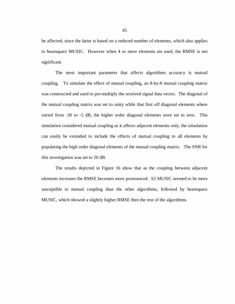
45
be affected, since the latter is based on a reduced number of elements, which also applies
to beamspace MUSIC. However when 4 or more elements are used, the RMSE is not
significant.
The most important parameter that affects algorithms accuracy is mutual
coupling. To simulate the effect of mutual coupling, an 8-by-8 mutual coupling matrix
was constructed and used to pre-multiply the received signal data vector. The diagonal of
the mutual coupling matrix was set to unity while that first off diagonal elements where
varied from -30 to -5 dB, the higher order diagonal elements were set to zero. This
simulation considered mutual coupling as it affects adjacent elements only, the simulation
can easily be extended to include the effects of mutual coupling to all elements by
populating the high order diagonal elements of the mutual coupling matrix. The SNR for
this investigation was set to 20 dB.
The results depicted in Figure 16 show that as the coupling between adjacent
elements increases the RMSE becomes more pronounced. S2 MUSIC seemed to be more
susceptible to mutual coupling than the other algorithms, followed by beamspace
MUSIC, which showed a slightly higher RMSE then the rest of the algorithms.

46
Figure 16 RMSE of different algorithms for varying mutual coupling
Phase and Magnitude Error Effect on Accuracy
The accuracy of the algorithms was examined as phase and amplitude errors were
introduced. The “rand” function in Matlab was used to simulate the phase and magnitude
errors. The function generates pseudo-random values drawn from a uniform distribution
on the unit interval. The SNR was set to 20dB and 1000 samples were used for the 8
element UCA. The phase error was varied from 5 degrees to 60 degrees in 5 degree
steps. The amplitude error was introduced as a percentage of the actual amplitude and
was varied from 5% to 50% in 5% increments. The RMSE was computed over 20 runs
for each phase and magnitude error.
Figure 17 depicts the RMSE vs. phase error showing a steady increase in RMSE
as the phase error increases. Results for S2 MUSIC showed a slightly higher RMSE
-30 -25 -20 -15 -10 -50
0.1
0.2
0.3
0.4
0.5
0.6
0.7Effect of Mutual coupling on accuracy of different algorithms
Adjacent elements mututal coupling (dB)
RM
SE (d
egre
es)
BartlettCaponMUSICBeamspace MUSICS2 MUSIC

47
compared to the other algorithms. Figure 18 shows the amplitude error, where capon and
beamspace MUSIC were the only algorithms where the amplitude RMSE was observed.
Figure 17 RMSE for different algorithms for a varyinginduced phase error
Figure 18 RMSE for different algorithms for a varyinginduced amplitude error
0 10 20 30 40 50 600.1
0.2
0.3
0.4
0.5
0.6
0.7
0.8
Induced Phase Error(degrees)
RM
SE (d
egre
es)
Robustness to phase error
BartlettcaponMUSICBeamSpace MUSICS2 MUSIC
5 10 15 20 25 30 35 40 45 50
0
0.02
0.04
0.06
0.08
0.1
0.12
0.14
Induced Phase Error (Percentage)
RM
SE (d
egre
es)
Robustness to Amplitude error (20dB)
BartlettBeamspace MUSICCapon
Induced amplitude error (degrees)

48
Resolution
To investigate how various parameters in the system affect the resolution of
algorithms, two sources (sinwaves) set 10 MHz apart were used in the simulation. One
of the sources was fixed at 180 degrees while the other was swept over the entire azimuth
range in 1 degree increments. The number of samples used was 1000 and azimuth range
was divided into 360 sectors. The results here are based on a single run; Monte Carlo
simulations should be carried out in the future to further validate the results. For S2
MUSIC, 5 elements were used and 7 beams were used in beamspace MUSIC. The first
parameter considered was SNR, where it was varied from 20 dB to 0 dB in 5 dB
increments.
Two types of plots are used to better visualize the results. The first is a histogram
of the bearings detected, with the y axis representing the fixed source while the x axis
represents the actual detected bearing, which corresponds to the peak that has the highest
power in the spectrum or the spatial pseudo-spectrum. The second plot, which is based
on the same results, is a power color map that enables one to visualize the power levels
for each of the signal sources detected over the entire azimuth range.
Only 20 dB SNR and 0 dB SNR results are shown, the rest of the results for SNR
15 dB, 10 dB, and 5 dB are included in Appendix D. Figure 19 depicts the histogram of
the results for 20dB and Figure 20 depicts the results for 0 dB. In the case where the
SNR is 20 dB, except Bartlett, all the algorithms seemed to have superb resolution at high
SNR. A closer look at the data revealed that Bartlett cannot resolve signals that are less

49
than 40 degree apart, while the Capon results show that it can resolve signals that are
spatially separated by more than 4 degrees.
Figure 19 Various algorithms histogram for an SNR of 20 dB
Figure 20 Various algorithms histogram for an SNR of 0 dB
Bartlett HistogramS
et A
ngle
[deg
]
Detected Angle [deg]50 100 150 200 250 300 350
100
200
300
Capon Histogram
Set
Ang
le [d
eg]
Detected Angle [deg]50 100 150 200 250 300 350
100
200
300
MUSIC Histogram
Set A
ngle
[deg
]
Detected Angle [deg]50 100 150 200 250 300 350
100
200
300
Beamspace MUSIC Histogram
Set A
ngle
[deg
]
Detected Angle [deg]50 100 150 200 250 300 350
100
200
300
S2 MUSIC Histogram (5 elements)
Set
Ang
le [d
eg]
Detected Angle [deg]50 100 150 200
50
100
150
200
SNR = 20dB
Bartlett Histogram
Set A
ngle
[deg
]
Detected Angle [deg]50 100 150 200 250 300 350
100
200
300
ML Histogram
Set A
ngle
[deg
]
Detected Angle [deg]50 100 150 200 250 300 350
100
200
300
MUSIC Histogram
Set A
ngle
[deg
]
Detected Angle [deg]50 100 150 200 250 300 350
100
200
300
Beamspace MUSIC Histogram
Set A
ngle
[deg
]
Detected Angle [deg]50 100 150 200 250 300 350
100
200
300
MUSIC Histogram (5 elements)
Set A
ngle
[deg
]
Detected Angle [deg]50 100 150 200
50
100
150
200
SNR = 0 dB

50
MUSIC, S2 MUSIC, and beamspace MUSIC all showed the ability to resolve the
two sources to within a degree at high SNR. At 0dB SNR, the ability to resolve spatially
close sources was dramatically affected. Bartlett could not resolve signals that were less
than 70 degrees apart and the deviation from the true peak reached a maximum of 2
degrees. Capon was unable to distinguish sources less than 54 degrees apart with a
maximum deviation from the true angle of 3 degrees. MUSIC exhibited the best
behavior with the ability to resolve to within 19 degrees and 2 degrees of maximum
deviation. Beamspace MUSIC failed to resolve signals within 27 degrees of spatial
separation with a maximum deviation of 3 degrees. S2 MUSIC achieved the same
resolution as MUSIC (20 degrees) but showed a maximum deviation error of 8 degrees.
In Figure 21 (SNR 20 dB) and Figure 22 (SNR 0 dB), the power of the spectrum
for each run over the entire field of view is plotted with a power color map. At 20 dB
SNR, the detected power spectrums obtained by using Bartlett revealed that the peaks
tend to merge at a faster rate compared to the other algorithms; the color map reveals that
the level of the sidelobes is very high. The other algorithms showed a good peak
separation along with a large peak to floor ratio, particularly for the high resolution
algorithms. Compared to the 20 dB SNR case, the 0 dB SNR case showed that as the
SNR decreases, the floor rises making the peak to floor ratio lower, affecting the
resolution performance. The histogram of S2 MUSIC is depicted in Figure 23.

51
Figure 21 Power color map plot for various algorithms with a set SNR of 20 dB
Figure 22 Power color map plot for various algorithms with a set SNR of 20 dB
Bartlett peak power
Set A
ngle
[deg
]
Detected Angle [deg]50 100 150 200 250 300 350
100
200
300
Capon peak power
Set A
ngle
[deg
]
Detected Angle [deg]50 100 150 200 250 300 350
100
200
300
MUSIC peak power
Set A
ngle
[deg
]
Detected Angle [deg]50 100 150 200 250 300 350
100
200
300
Beamspace peak Mean power
Set A
ngle
[deg
]
Detected Angle [deg]50 100 150 200
100
200
300
S2-MUSIC peak power
Set A
ngle
[deg
]
Detected Angle [deg]50 100 150 200
100
200
300-60
-40
-20
0
SNR = 20 dB
Bartlett peak power
Set A
ngle
[deg
]
Detected Angle [deg]50 100 150 200 250 300 350
100
200
300
Capon peak power
Set A
ngle
[deg
]
Detected Angle [deg]50 100 150 200 250 300 350
100
200
300
MUSIC peak power
Set A
ngle
[deg
]
Detected Angle [deg]50 100 150 200 250 300 350
100
200
300
Beamspace MUSIC peak power
Set A
ngle
[deg
]
Detected Angle [deg]50 100 150 200
100
200
300
S2-MUSIC peak power
Set A
ngle
[deg
]
Detected Angle [deg]50 100 150 200
100
200
300-60
-50
-40
-30
-20
-10
0
SNR = 0 dB

52
Figure 23 Histogram for S2 MUSIC for varying SNR
Figure 23 shows how S2 MUSIC is affected by varying the SNR for a fixed
number of elements (5 elements). Above 10 dB SNR, the algorithm behaves well in
terms of resolution and accuracy, but below 10 dB SNR the ability to resolve closely
spaced sources is diminished along with noticeable degradation in accuracy.
The next step consisted of investigating how the number of samples used affects
the resolution of the algorithms. In this case, the SNR was fixed at 20 dB, 5 elements
were used for S2 MUSIC and 7 beams were used for beamspace MUSIC. The number of
samples were 10, 100, and 1000. The results in a histogram format that show the set
angle vs. the detected angle are depicted in Figure 24, Figure 25, and Figure 26,
respectively. Comparing 10 sample and 100 sample results, it is clear that a low sample
number tends to degrade the resolution capability of all the algorithms. Capon in
S2 MUSIC Histogram, SNR 20
Set A
ngle
[deg
]
Detected Angle [deg]50 100 150 200
50
100
150
200
S2 MUSIC Histogram, SNR 15
Set A
ngle
[deg
]
Detected Angle [deg]50 100 150 200
50
100
150
200
S2 MUSIC Histogram, SNR 10
Set A
ngle
[deg
]
Detected Angle [deg]50 100 150 200
50
100
150
200
S2 MUSIC Histogram, SNR 5
Set A
ngle
[deg
]
Detected Angle [deg]50 100 150 200
50
100
150
200
S2 MUSIC Histogram, SNR 0
Set A
ngle
[deg
]
Detected Angle [deg]50 100 150 200
50
100
150
200

53
particular resulted in more false peaks than any other algorithm. The results obtained
when 1000 samples were used are comparable to when 100 samples were used.
The number of adjacent elements in the array was also varied to examine its effect
on resolution. The SNR was set to 10 dB, 1000 samples were used and 7 beams were
used for beamspace MUSIC. The results when the number of elements used was 4, 6,
and 10 are presented in Figure 27, Figure 28, and Figure 29, respectively. It is clear that
as the number of elements increases, the resolution is improved. Bartlett showed the
largest effect since its resolution is directly dependent on the number of elements used.
Capon resulted in a better resolution than Bartlett and was more affected by the decrease
in the number of elements than the high resolution algorithms.
Figure 24 Histogram for various algorithms for a receiveddata vector sampled 10 times
Bartlett Histogram
Set A
ngle
[deg
]
Detected Angle [deg]50 100 150 200 250 300 350
100
200
300
Capon Histogram
Set A
ngle
[deg
]
Detected Angle [deg]50 100 150 200 250 300 350
100
200
300
MUSIC Histogram
Set A
ngle
[deg
]
Detected Angle [deg]50 100 150 200 250 300 350
100
200
300
Beamspace MUSIC Histogram
Set A
ngle
[deg
]
Detected Angle [deg]50 100 150 200 250 300 350
100
200
300
S2 MUSIC Histogram
Set A
ngle
[deg
]
Detected Angle [deg]50 100 150 200
50
100
150
200
10 Samples

54
Figure 25 Histogram for various algorithms for a receiveddata vector sampled 100 times
Figure 26 Histogram for various algorithms for a receiveddata vector sampled 1000 times
Bartlett Histogram
Set A
ngle
[deg
]
Detected Angle [deg]50 100 150 200 250 300 350
100
200
300
Capon Histogram
Set A
ngle
[deg
]
Detected Angle [deg]50 100 150 200 250 300 350
100
200
300
MUSIC Histogram
Set A
ngle
[deg
]
Detected Angle [deg]50 100 150 200 250 300 350
100
200
300
Beamspace MUSIC Histogram
Set A
ngle
[deg
]
Detected Angle [deg]50 100 150 200 250 300 350
100
200
300
S2 MUSIC Histogram
Set A
ngle
[deg
]
Detected Angle [deg]50 100 150 200
50
100
150
200
100 Samples
Bartlett Histogram
Set A
ngle
[deg
]
Detected Angle [deg]50 100 150 200 250 300 350
100
200
300
Capon Histogram
Set A
ngle
[deg
]
Detected Angle [deg]50 100 150 200 250 300 350
100
200
300
MUSIC Histogram
Set A
ngle
[deg
]
Detected Angle [deg]50 100 150 200 250 300 350
100
200
300
Beamspace MUSIC Histogram
Set A
ngle
[deg
]
Detected Angle [deg]50 100 150 200 250 300 350
100
200
300
S2 MUSIC Histogram
Set
Ang
le [d
eg]
Detected Angle [deg]50 100 150 200
50
100
150
200
1000 Samples

55
Figure 27 Histogram for various algorithms when a 4 element UCA is used
Figure 28 Histogram for various algorithms when a 6 element UCA is used
Bartlett Histogram
Set A
ngle
[deg
]
Detected Angle [deg]50 100 150 200 250 300 350
50
100
150
200
250
300
350
Capon Histogram
Set A
ngle
[deg
]
Detected Angle [deg]50 100 150 200 250 300 350
50
100
150
200
250
300
350
MUSIC Histogram
Set A
ngle
[deg
]
Detected Angle [deg]50 100 150 200 250 300 350
50
100
150
200
250
300
350
Beamspace MUSIC Histogram
Set A
ngle
[deg
]
Detected Angle [deg]50 100 150 200 250 300 350
50
100
150
200
250
300
350
4 elements
Bartlett Histogram
Set A
ngle
[deg
]
Detected Angle [deg]50 100 150 200 250 300 350
50
100
150
200
250
300
350
Capon Histogram
Set A
ngle
[deg
]
Detected Angle [deg]50 100 150 200 250 300 350
50
100
150
200
250
300
350
MUSIC Histogram
Set A
ngle
[deg
]
Detected Angle [deg]50 100 150 200 250 300 350
50
100
150
200
250
300
350
Beamspace MUSIC Histogram
Set A
ngle
[deg
]
Detected Angle [deg]50 100 150 200 250 300 350
50
100
150
200
250
300
350
6 elements

56
Figure 29 Histogram for various algorithms when a 10 element UCA is used
Robustness Towards Phase and Magnitude Error
In this section the resilience of the algorithms when subjected to phase and
magnitude error is examined. Figure 30, Figure 32, and Figure 34 represent the
histogram results for the set angle vs. the detected angle when the induced angle error
was set to 5 degrees, 20 degrees, and 40 degrees, respectively. The power color map
plots are shown in Figure 31, Figure 33, and Figure 35 for the same simulation
conditions. The results indicate that at as the phase error is increased, resolution
capability is reduced and the floor rises significantly. In addition, the accuracy is affected
and the algorithms’ error increased significantly with an increased phase error. S2
MUSIC was affected the most compared to the other high resolution algorithms because
less elements were used.
Bartlett Histogram
Set A
ngle
[deg
]
Detected Angle [deg]50 100 150 200 250 300 350
50
100
150
200
250
300
350
Capon Histogram
Set A
ngle
[deg
]
Detected Angle [deg]50 100 150 200 250 300 350
50
100
150
200
250
300
350
MUSIC Histogram
Set A
ngle
[deg
]
Detected Angle [deg]50 100 150 200 250 300 350
50
100
150
200
250
300
350
Beamspace MUSIC Histogram
Set A
ngle
[deg
]Detected Angle [deg]
50 100 150 200 250 300 350
50
100
150
200
250
300
350
10 elements

57
Figure 30 Histogram for various algorithms when a 5 degree phase error is induced
Figure 36, Figure 38, and Figure 40, respectively, show the histogram results
when 5%, 20% and 40% amplitude error is introduced. Figure 37, Figure 39, and Figure
41show the power color map when the amplitude error was varied from 5%, 20%, to 40%
respectively. The results indicate that the resolution of the algorithms along with the
peak-to-floor ratio deteriorate as the amplitude error is increased, and S2 MUSIC seemed
the least resilient to amplitude error.
Bartlett Histogram 5deg error 20dB
Set A
ngle
[deg
]
Detected Angle [deg]100 150 200 250
100
150
200
250
Capon Histogram 5deg error 20dB
Set A
ngle
[deg
]
Detected Angle [deg]100 150 200 250
100
150
200
250
MUSIC Histogram 5deg error 20dB
Set A
ngle
[deg
]
Detected Angle [deg]100 150 200 250
100
150
200
250
Beamspace Histogram 5deg error 20dB
Set A
ngle
[deg
]
Detected Angle [deg]100 150 200 250
100
150
200
250
S2 MUSIC Histogram 5deg error 20dB
Set A
ngle
[deg
]
Detected Angle [deg]120 140 160 180 200 220
100
150
200
250
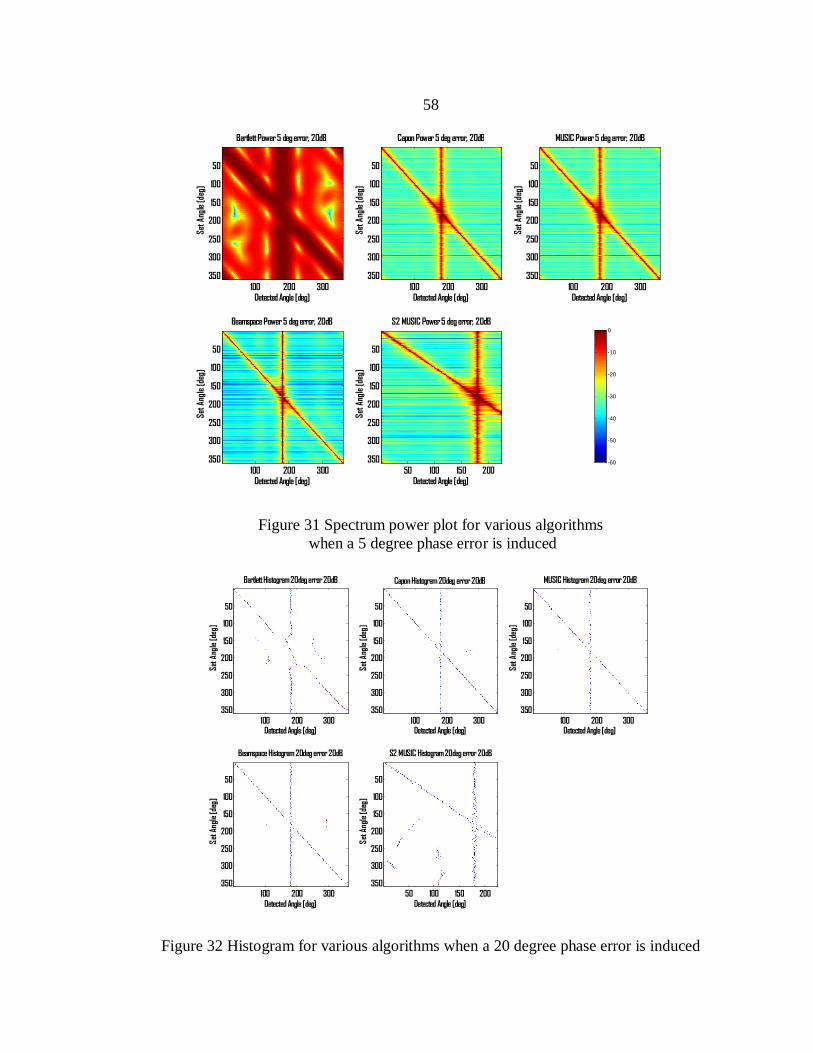
58
Figure 31 Spectrum power plot for various algorithms when a 5 degree phase error is induced
Figure 32 Histogram for various algorithms when a 20 degree phase error is induced
Bartlett Power 5 deg error, 20dB
Set A
ngle
[deg
]
Detected Angle [deg]100 200 300
50
100
150
200
250
300
350
Capon Power 5 deg error, 20dB
Set A
ngle
[deg
]
Detected Angle [deg]100 200 300
50
100
150
200
250
300
350
MUSIC Power 5 deg error, 20dB
Set A
ngle
[deg
]
Detected Angle [deg]100 200 300
50
100
150
200
250
300
350
Beamspace Power 5 deg error, 20dB
Set A
ngle
[deg
]
Detected Angle [deg]100 200 300
50
100
150
200
250
300
350
S2 MUSIC Power 5 deg error, 20dB
Set A
ngle
[deg
]
Detected Angle [deg]50 100 150 200
50
100
150
200
250
300
350 -60
-50
-40
-30
-20
-10
0
Bartlett Histogram 20deg error 20dB
Set A
ngle
[deg
]
Detected Angle [deg]100 200 300
50
100
150
200
250
300
350
Capon Histogram 20deg error 20dB
Set A
ngle
[deg
]
Detected Angle [deg]100 200 300
50
100
150
200
250
300
350
MUSIC Histogram 20deg error 20dB
Set A
ngle
[deg
]
Detected Angle [deg]100 200 300
50
100
150
200
250
300
350
Beamspace Histogram 20deg error 20dB
Set A
ngle
[deg
]
Detected Angle [deg]100 200 300
50
100
150
200
250
300
350
S2 MUSIC Histogram 20deg error 20dB
Set A
ngle
[deg
]
Detected Angle [deg]50 100 150 200
50
100
150
200
250
300
350

59
Figure 33 Spectrum power plot for various algorithms when a 20 degree phase error is induced
Figure 34 Histogram for various algorithms when a 40 degree phase error is induced
Bartlett Power 20 deg error, 20dB
Set A
ngle
[deg
]
Detected Angle [deg]100 200 300
50
100
150
200
250
300
350
Capon Power 20 deg error, 20dB
Set A
ngle
[deg
]
Detected Angle [deg]100 200 300
50
100
150
200
250
300
350
MUSIC Power 20 deg error, 20dB
Set A
ngle
[deg
]
Detected Angle [deg]100 200 300
50
100
150
200
250
300
350
Beamspace Power 20 deg error, 20dB
Set A
ngle
[deg
]
Detected Angle [deg]100 200 300
50
100
150
200
250
300
350
S2 MUSIC Power 20 deg error, 20dB
Set A
ngle
[deg
]
Detected Angle [deg]50 100 150 200
50
100
150
200
250
300
350 -60
-50
-40
-30
-20
-10
0
Bartlett Histogram 40deg error 20dB
Set A
ngle
[deg
]
Detected Angle [deg]100 200 300
50
100
150
200
250
300
350
Capon Histogram 40deg error 20dB
Set A
ngle
[deg
]
Detected Angle [deg]100 200 300
50
100
150
200
250
300
350
MUSIC Histogram 40deg error 20dB
Set A
ngle
[deg
]
Detected Angle [deg]100 200 300
50
100
150
200
250
300
350
Beamspace Histogram 40deg error 20dB
Set A
ngle
[deg
]
Detected Angle [deg]100 200 300
50
100
150
200
250
300
350
S2 MUSIC Histogram 40deg error 20dB
Set A
ngle
[deg
]
Detected Angle [deg]50 100 150 200
50
100
150
200
250
300
350

60
Figure 35 Spectrum power plot for various algorithmswhen a 40 degree phase error is induced
Figure 36 Histogram for various algorithms when a 5% amplitude error is induced
Bartlett Power 40 deg error, 20dB
Set A
ngle
[deg
]
Detected Angle [deg]100 200 300
50
100
150
200
250
300
350
Capon Power 40 deg error, 20dB
Set A
ngle
[deg
]
Detected Angle [deg]100 200 300
50
100
150
200
250
300
350
MUSIC Power 40 deg error, 20dB
Set A
ngle
[deg
]
Detected Angle [deg]100 200 300
50
100
150
200
250
300
350
Beamspace Power 40 deg error, 20dB
Set A
ngle
[deg
]
Detected Angle [deg]100 200 300
50
100
150
200
250
300
350
S2 MUSIC Power 40 deg error, 20dB
Set A
ngle
[deg
]
Detected Angle [deg]50 100 150 200
50
100
150
200
250
300
350 -60
-50
-40
-30
-20
-10
0
Bartlett Histogram 5% error 20dB
Set A
ngle
[deg
]
Detected Angle [deg]100 150 200 250
100
150
200
250
Capon Histogram 5% error 20dB
Set A
ngle
[deg
]
Detected Angle [deg]100 150 200 250
100
150
200
250
MUSIC Histogram 5% error 20dB
Set A
ngle
[deg
]
Detected Angle [deg]100 150 200 250
100
150
200
250
Beamspace Histogram 5% error 20dB
Set A
ngle
[deg
]
Detected Angle [deg]100 150 200 250
100
150
200
250
S2 MUSIC Histogram 5% error 20dB
Set A
ngle
[deg
]
Detected Angle [deg]120 140 160 180 200 220
100
150
200
250

61
Figure 37 Spectrum power plot for various algorithmswhen a 5% amplitude error is induced
Figure 38 Histogram for various algorithms when a 20% amplitude error is induced
Bartlett Power 5% error, 20dB
Set A
ngle
[deg
]
Detected Angle [deg]100 200 300
50
100
150
200
250
300
350
Capon Power 5% error, 20dB
Set A
ngle
[deg
]
Detected Angle [deg]100 200 300
50
100
150
200
250
300
350
MUSIC Power 5% error, 20dB
Set A
ngle
[deg
]
Detected Angle [deg]100 200 300
50
100
150
200
250
300
350
Beamspace Power 5% error, 20dB
Set A
ngle
[deg
]
Detected Angle [deg]100 200 300
50
100
150
200
250
300
350
S2 MUSIC Power 5% error, 20dB
Set A
ngle
[deg
]
Detected Angle [deg]50 100 150 200
50
100
150
200
250
300
350-60
-50
-40
-30
-20
-10
0
Bartlett Histogram 20% error 20dB
Set A
ngle
[deg
]
Detected Angle [deg]100 150 200 250
100
150
200
250
Capon Histogram 20% error 20dB
Set A
ngle
[deg
]
Detected Angle [deg]100 150 200 250
100
150
200
250
MUSIC Histogram 20% error 20dB
Set A
ngle
[deg
]
Detected Angle [deg]100 150 200 250
100
150
200
250
Beamspace Histogram 20% error 20dB
Set A
ngle
[deg
]
Detected Angle [deg]100 150 200 250
100
150
200
250
S2 MUSIC Histogram 20% error 20dB
Set A
ngle
[deg
]
Detected Angle [deg]120 140 160 180 200 220
100
150
200
250

62
Figure 39 Spectrum power plot for various algorithmswhen a 20% amplitude error is induced
Figure 40 Histogram for various algorithms when 40% amplitude error is induced
Bartlett Power 20% error, 20dB
Set A
ngle
[deg
]
Detected Angle [deg]100 200 300
50
100
150
200
250
300
350
Capon Power 20% error, 20dB
Set A
ngle
[deg
]
Detected Angle [deg]100 200 300
50
100
150
200
250
300
350
MUSIC Power 20% error, 20dB
Set A
ngle
[deg
]
Detected Angle [deg]100 200 300
50
100
150
200
250
300
350
Beamspace Power 20% error, 20dB
Set A
ngle
[deg
]
Detected Angle [deg]100 200 300
50
100
150
200
250
300
350
S2 MUSIC Power 20% error, 20dB
Set A
ngle
[deg
]
Detected Angle [deg]50 100 150 200
50
100
150
200
250
300
350-60
-50
-40
-30
-20
-10
0
Bartlett Histogram 40% error 20dB
Set A
ngle
[deg
]
Detected Angle [deg]100 150 200 250
100
150
200
250
Capon Histogram 40% error 20dB
Set A
ngle
[deg
]
Detected Angle [deg]100 150 200 250
100
150
200
250
MUSIC Histogram 40% error 20dB
Set A
ngle
[deg
]
Detected Angle [deg]100 150 200 250
100
150
200
250
Beamspace Histogram 40% error 20dB
Set A
ngle
[deg
]
Detected Angle [deg]100 150 200 250
100
150
200
250
S2 MUSIC Histogram 40% error 20dB
Set A
ngle
[deg
]
Detected Angle [deg]120 140 160 180 200 220
100
150
200
250
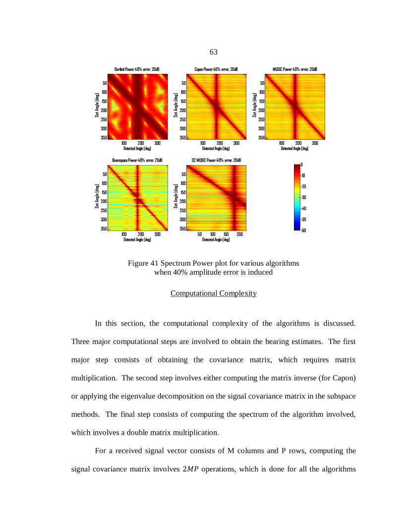
63
Figure 41 Spectrum Power plot for various algorithmswhen 40% amplitude error is induced
Computational Complexity
In this section, the computational complexity of the algorithms is discussed.
Three major computational steps are involved to obtain the bearing estimates. The first
major step consists of obtaining the covariance matrix, which requires matrix
multiplication. The second step involves either computing the matrix inverse (for Capon)
or applying the eigenvalue decomposition on the signal covariance matrix in the subspace
methods. The final step consists of computing the spectrum of the algorithm involved,
which involves a double matrix multiplication.
For a received signal vector consists of M columns and P rows, computing the
signal covariance matrix involves 2 operations, which is done for all the algorithms
Bartlett Power 40% error, 20dB
Set A
ngle
[deg
]
Detected Angle [deg]100 200 300
50
100
150
200
250
300
350
Capon Power 40% error, 20dB
Set A
ngle
[deg
]
Detected Angle [deg]100 200 300
50
100
150
200
250
300
350
MUSIC Power 40% error, 20dB
Set A
ngle
[deg
]
Detected Angle [deg]100 200 300
50
100
150
200
250
300
350
Beamspace Power 40% error, 20dB
Set A
ngle
[deg
]
Detected Angle [deg]100 200 300
50
100
150
200
250
300
350
S2 MUSIC Power 40% error, 20dB
Set A
ngle
[deg
]
Detected Angle [deg]50 100 150 200
50
100
150
200
250
300
350 -60
-50
-40
-30
-20
-10
0

64
except S2 MUSIC. Since only a limited number of elements is chosen for S2 MUSIC
(usually half of the elements compared to other algorithms) an obvious computational
reduction is obtained when S2 MUSIC is used. Once the signal covariance matrix is
obtained, the inverse or eigenvalue decomposition which is of ( ) is computed.
Reducing the number of elements in S2 MUSIC is analogous to a reduced covariance
matrix size, and with ( ) the computational reduction is significant. The final stage
consists of obtaining the spatial pseudo-spectrum. The conjugate transpose of the
steering vector[ × ] is multiplied by the noise covariance matrix (also reduced in the
case of S2 MUSIC), and the result is then multiplied by the steering vector of size [ ×
], where S is the number of sectors used to quantize the azimuth range. The required
number of operations is 4 , in addition to the computation needed to obtain the noise
covariance matrix. In this step S2 MUSIC saves computation not only in obtaining the
noise covariance matrix, but also in obtaining the spectrum, since the number of sectors S
is reduced significantly (at least by half).
When beamspace is used, the received signal vector is pre-multiplied by a
beamformer matrix, and depending on the number of modes used, the size of the
covariance matrix is reduced (when 3 modes are used corresponding to 7 beams the
covariance matrix is reduced by one). Compared to beamspace MUSIC, S2 MUSIC is
more computationally efficient since it does not require pre-multiplying the receiver data
vector by the beamformer matrix, in addition to the fact that S2 MUSIC uses a reduced
number of sectors in obtaining the spatial pseudo-spectrum, which is not the case for
beamspace MUSIC.

65
All the above observations lead to one conclusion, S2 MUSIC is computationally
more efficient than MUSIC and beamspace MUSIC because both the number of elements
used and the number of sectors are reduced, which leads to less computational burden
when obtaining the DOA estimates.
Simulation Results Discussion
In this chapter, the accuracy and resolution of the algorithms have been
investigated for a variety of parameters. The results indicated that under low SNR the
algorithm accuracy and resolution are affected dramatically, suggesting that when
building the necessary hardware, The SNR needs to be high enough to mitigate its effects
on the DOA estimates. Phase error affected the accuracy and resolution of the algorithms
more so than amplitude error, pointing out that proper design of the hardware and
accurate phase calibration will be imperative to reaching high resolution DOA estimates.
When S2 MUSIC is used, 4 elements or more are needed, since using a lower
number will cause significant error in accuracy and cause degradation in resolving
azimuthally close sources. Another note worth mentioning concerns the relationship
between the peak-to-floor ratio and resolution capability of the algorithms. It was clear
from the simulations that when the measurement floor rises, it causes a decrease in the
resolution capability of the algorithms. It was evident that using a low number of
samples cause errors in the estimates and resolution, so using a large number of signal
samples is also important. Mutual coupling was also investigated and simulation results
showed that even at very high SNR, it caused a significant error in accuracy. Finally, the

66
examination of computational efficiency indicates that S2 MUSIC is significantly more
efficient in terms of computation when compared to the other high resolution algorithms.
Though S2 MUSIC is more susceptible to low SNR and mutual coupling, its performance
is comparable to the conventional MUSIC.
In the next chapter, the design and implementation of the necessary hardware to
achieve high resolution DOA estimation a discussed. How to mitigate the phase errors in
the system along with mutual coupling is also investigated.

67
CHAPTER FOUR
HARDWARE DESIGN AND IMPLEMENTATION
Many issues face engineers when designing receivers. The challenges do change
with the application but some issues are to be addressed in any situation. The dual goals
of making a receiver that exhibits high dynamic range while being very sensitive are
indeed hard to achieve. The power of the signals of interest might vary from very high to
the point of causing saturation to the input sensitive components, to very low making the
signal hard to distinguish from noise. A high dynamic range receiver is necessary to
avoid non-linear affects which can drive the circuits into compression, which decreases
the gain, and can bias results where amplitude measurements are a consideration.
When GHz RF signals are of interest, mixing usually takes place in the receiver
and causes a multitude of issues. Heterodyne mixing in particular causes intermodulation
and the IF has to be carefully placed to avoid being in the vicinity of harmonics resulting
from the mixing operation. In addition, LO re-radiation causes major issues. Leakage
from the local oscillator seeps out to the antenna causing unwanted radiation at the
antenna in the receiving mode. Proper filtering should also be considered to avoid
aggregate noise build up on the RF and IF sides. In the case where direct conversion is
used, going from RF to baseband without the intermediate IF stage, the lower sideband
folds over and causes signal interference.
The 8-channel receiver board, designed and implemented by the author, provides
the hardware piece responsible for taking the 5.8 GHz signal to baseband and delivering
the information to the DAQ card. A single stage image reject (IR) mixer was considered

68
to achieve frequency translation to baseband. The RF signal is filtered, amplified, and
filtered once again, and then mixed using a distributed local oscillator. The choice of the
baseband bandwidth is solely dependent on the speed at which one can digitize the
signals. The manual gain control settings are used to provide an acceptable level to the
DAQ card. A simplified block diagram for one channel is shown in Figure 42.
Figure 42 Simplified block diagram for one channel in the receiver board
The receiver board went through two design phases. In the first design, the
implementation was done in two stages, a dual channel board was first constructed and
each of the components was tested to make sure that the design parameters were met.
Once the two channels were tested successfully, the full 8-channel receiver board was
designed using PADS and fabricated. Troubleshooting revealed that on the RF side, the
pre-amplifier input and output ports were switched in the footprint requiring some repairs
which at 5.8 GHz causes major cross channel interference. In the first design, both the
LO drive and the variable gain amplifiers at IF were used as evaluation boards and were
RF Filter RF FilterPre-
amplifier
LocalOscillator
IF FilterAutomaticGain Amplifier
Signal Source(5.8 GHz)

69
not incorporated in the layout of the receiver board. Figure 43 illustrates the first version
of the receiver board.
Figure 43 Snapshot of the first revision of the receiver board
The second version was designed to include a multitude of improvements. The
upgrades consisted of improving the front end design (by including the low noise pre-
amp), incorporating an onboard phase locked loop (PLL) for computer controlled local
oscillator generation, incorporating onboard variable gain amplifiers with independent
gain control for channel gain matching, and adding switchable IF low pass anti-alias
filters to optimize for low speed or high speed data acquisition. A single PLL was used
for LO generation and symmetrically distributed to the eight channels. An alternate
approach that was not implemented consisted of including an individual PLL for each
channel controlled by a numerically controlled oscillator to individually adjust the
channel phases. This would have allowed for more flexibility at the expense of hardware
complexity. Thought was also given to make the receiver bidirectional by eliminating

70
the RF preamplifiers and including the ability to bypass the variable gain amplifier. The
translator could then be used both as a digital BF or a DOA estimation receiver. It was
decided that this can be considered in later revisions.
In the implementation of the receiver board, the printed circuit board (PCB)
material chosen was FR4 and cost was the main driver behind the choice. The overall
physical size of the board was determined by the connector spacing and shielding goals.
The main goals behind designing a board enclosure were to shield each of the 5.8 GHz
RF input channel from one another, and to provide mechanical rigidity to the board to
assure phase stability.
A total of four layers were used for the PCB. The top and bottom layers were
organized such that the RF components were on top and IF components were on bottom.
The ground layer was directly under the RF layer, followed by the power distribution
layer. To minimize the phase differences between channels, path symmetry was applied
to the LO distribution and to the RF input paths. A coplanar waveguide was used for the
5.8GHz signals. The board manufacturer, Prototron, provided the exact board properties
for calculating the correct line spacing and gap for a 50 Ohm system impedance.
Symmetry was also used on the IF side of the board to insure that all the IF channels are
in phase. The width of the traces on the RF side was calculated using AppCAD software
as shown in Figure 44, to achieve 50 ohm impedance given the material dielectric along
with the frequency of operation. The trace width along with the ground clearance was
calculated for the RF trace in the receiver board. Given the properties provided by the

71
manufacturer, the trace width was 0.022 inches and the gap between the trace and the
ground plane was 0.006 inches.
Figure 44 Example of use of AppCAD software to calculate the width and groundclearance for the RF traces in the receiver board
The wall thickness wes determined by the screws that were used to attach the top
and bottom lids. The enclosure was designed (by Aaron Traxinger) such that the
5.8GHz sections of the board are shielded from each other. Each side of the box has a lid
which enables easy access to the board when troubleshooting is required. The IF
connectors were designed to mate directly (without the need for cables) with the high
speed A/D board. The lid for the IF section was designed with a stepped lip to create
some shielding from external RF interference. Electromagnetic interference (EMI)
filtered power input terminals along with an EMI filtered RS232 port were used to
minimize external RF interference from infiltrating the enclosure. Closely spaced screws
were used to insure a tight connection to the exposed ground connection. Extra screws

72
were used in the RF section lid to minimize the amount of RF leakage between each RF
pocket.
A snap shot of the front side of the receiver board is depicted in Figure 45, where
the RF inputs are situated on left side. The RF channels were egg crated for channel-to-
channel isolation. The LO distribution is situated on the right side.
Figure 45 Snap shot of the front side of the receiver boardin the aluminum enclosure
Figure 46 depicts the back side of the receiver board which contains the IF
components. Starting from the right hand side the IF signal generated by the mixer is fed
to the variable gain amplifier chip and then the amplified IF signal is filtered either
though the 1MHz or 10 MHz lowpass filters.

73
Figure 46 Snap shot of the back side of the receiver boardin the aluminum enclosure
The following sections discuss the RF side, LO distribution, and IF side. Detailed
schematics of the second version receiver, along with the layout of the RF and IF layers,
a bill of materials, and the enclosure drawings are provided in Appendix A.
RF Side
The RF side of the receiver board includes the RF input and the LO distribution.
The 5.8 GHz signal(s) received by the array elements are fed to the receiver board via
SMA female connectors and the signal is filtered using a Johanson Technology, Inc P/N

74
5515BP15B725 filter. The bandpass filter operates from 5.150 GHz to 5.875 GHz,
introduces a maximum of 1.5 dB insertion loss and has a minimum return loss of 9.5 dB.
The signal is then amplified using an HMC318 Hittite amplifier. This low noise
amplifier was chosen for its low noise figure (2.5 dB) and excellent return loss
performance. It provides a typical gain of 9 dB. The signal is then filtered again and fed
to the RF input of the mixer. The HMC488 mixer was used, and is a double balanced
mixer with an integrated LO amplifier. The LO amplifier can be driven from 0 to +6
dBm and requires a single supply of +5V.
Each of the LO inputs of the mixers are fed through the on board LO distribution.
The LO signal is generated using the AD4106 PLL frequency synthesizer and the
incorporated LO design was borrowed from the Analog Devices EVAL-ADF411XEB1
evaluation board. A detailed schematic of the LO drive design is shown in Appendix A.
The LO signal is controlled using a PC interface provided by Analog Devices. The LO
signal is then distributed to all the LO input ports of the mixers with the help of a Mini-
Circuits GP2X+ power splitter/combiner. The power splitter is wideband (2.9 GHz to 6.2
GHz) and at 5.8 GHz the splitter has a typical isolation of 18.7 dB. It has an excellent
amplitude unbalance (0.05 dB typical) and good phase unbalance (3 degrees typical). At
each stage of the power division the Hittite HMC311 amplifier was used such that the
power of the signal matches the LO drive power required by the mixer.

75
IF Side
The IF side contains the variable gain amplifiers and the IF filters. Analog
Devices AD8334 variable gain amplifiers were used for this project. The AD8334 is a
quad-channel, ultralow noise variable gain amplifier with a 100 MHz 3dB bandwidth.
The datasheet specifies that this amplifier can produce up to 55.5 dB of gain, but this
statement is not totally valid since with the proper output matching network only 30 dB
of gain can be achieved. One can, however, increase the gain of the amplifier by
reducing the resistance values of the output matching network. A detailed schematic of
the variable gain amplifiers is shown in Appendix A.
Two IF filters paths were used on this board to accommodate for low and high
speed data acquisition. The filters used were designed with the help of the Genesys
software. The filters are a 3 pole traditional (or Butterworth) design and the schematics
of the filters are given in Appendix A.
Receiver Board and Performance
The receiver board DC power is provided by two regulated voltage supplies, +5V
and +3V. According to the specifications provided by the components’ manufacturers,
the board should draw 70 mA at 3 V and 736 mA at 5 V, and the total power consumed
by the receiver board is 3.89 watts. The board’s actual current draw is 889 mA, higher
than expected because typical specifications were used. The RF conversion loss was
measured to be -1 dB, and the IF section was also tested and showed 30.5 dB gain at each
channel. If more gain is needed, the matching network at the output of the variable gain

76
amplifier can be modified, that will cause some mismatch but can results in a higher gain.
Tests with the frequency synthesizer showed noisy behavior and inability of the PLL to
lock. This problem was solved by adding the appropriate capacitance to the regulator
terminals to filter out the noise leaking into the synthesizer. The RF channel-to-channel
isolation was measured using the HP 8720D network analyzer, and isolation between
adjacent channels was measured to be in excess of 65 dB.
The receiver board magnitude and phase behavior tests were carried out after
accomplishing the basic RF, IF, and LO functionality tests. The set up consisted of the
Anritsu 68369 function generator as the RF input, and the signal from the function
generator was divided using the Mini-Circuit ZX10R-14-S+ splitter. Channel 1 of the
receiver board was used as the reference while the unused channels were terminated. The
Tektronix TDS 3054B oscilloscope was used to measure the output signals (16 point
averaging was used when the data was recorded). The power at the input of the receiver
was set to -40dBm. The test was carried out for both the 1 MHz channels and the 10
MHz channels and channel-to-channel phase and magnitude variations were recorded as
the IF bandwidth was varied. For the 1MHz Channels, the IF frequency was varied from
100KHz to 1500 KHz in 100 KHz steps while for the 10 MHz channel the IF bandwidth
was varied from 1MHz to 15 MHz in 1 MHz steps. The center frequency was set to 5.8
GHz and the synthesizer frequency was varied accordingly to provide the appropriate
baseband frequency. Measurements for the 1 MHz channels are shown in Table 1, where
all the phase measurements are relative to channel 1 and the magnitude variation for
channel 1 is shown in Table 2. Phase variations vs. the IF frequencies are plotted in

77
Figure 47 (relative to channel 1). For the 10 MHz channels, the measurements are shown
in Table 3 and Table 4 shows the amplitude variation for channel 1. Measurements
indicate that the amplitude variation is less than 2 dB from the channel exhibiting the
largest voltage to the one showing the lowest in both the 1 MHz and 10 MHz channels.
The relative phase difference is very stable at about 500 KHz in the 1 MHz channels and
at about 5 MHz in the 10 MHz channels. Beyond that point the relative phase difference
varied dramatically. This variation is due to the IF filters not having a matching
frequency response, since each filter, due to the tolerance of the parts exhibits a different
ripple effect along with a different 3dB point. The difference in amplitude caused by the
ripple effect in the filters translates into phase differences. For the DOA estimation
algorithms, precise knowledge of the phase and amplitude is imperative for good
performance. To avoid phase variations within the IF band, the filters should be designed
with a 3dB bandwidth twice as big as the desired IF bandwidth to avoid the ripple effect
and obtain a flat phase response within the band of interest.

78
Table 1 Magnitude and phase variation for all channels for different IF frequency (1MHz), magnitudes are recorded in mV and the angles are recorded in degrees
Frequency (KHz)
Channel 2 Channel 3 Channel 4 Channel 5 Channel 6 Channel 7 Channel 8Mag Ang Mag Ang Mag Ang Mag Ang Mag Ang Mag Ang Mag Ang
100 133.7 -10.5 120 -11.9 106 -22.7 116 34 120 19.5 111.3 37.5 111.7 30200 131.5 -10.7 118.8 -12.0 104.3 -22 114 34 118.5 20 110 37.1 107 29.1300 136.7 -10.7 124 -11.5 108 -22 118 34.9 122.7 20 114 37.9 108 28400 147.4 -10.7 133.2 -10.5 116.3 -22.2 127.4 35.5 131.8 20.5 124 38 111.7 26.7500 164.8 -9.0 150.1 -9 130 -21 143 37.5 147.7 22 140 41.5 119 23.5600 184.5 -7.0 167.5 -6.7 146 -20 160 40 167 24.5 158 43.5 131.4 19700 194 -4.5 174.8 -3 156 -17 168 44 175.7 28 165 48.5 145.8 14.5800 185.7 -2.5 165 -1.5 150 -15 158 45.5 167 30 155.8 50 153.5 14900 175.4 0 154 0 139 -12 147 48.5 157 33 146 52 149.2 171000 183.3 +7.5 162 7 142 -6.5 154 55 165.4 40 154 59 140 22.81100 217.8 +36 200 36 172.8 15 189 84 199 70 189 90 138 26.51200 150 76 134 80 137 59 127 128 130 112 121.8 132 158 291300 70 41 60 44 62 30 56 90 60 75 54.6 94 175 171400 35 4 30 7 30 -5 28 54 29.5 38 27 57 95 181500 19.6 -5 16 -4.5 16.9 -15 15 42 17 27 15.3 46 42 20
Table 2 Channel 1 amplitude variation for different IF frequency (1MHz)
Channel 1(KHz)
Mag(mV)
100 129200 125300 128400 135500 145.8600 159700 164800 152.2900 134.51000 121.61100 122.91200 152.81300 177.31400 85.81500 39.9

79
Figure 47 Plot of phase variation for all channels relative to channels for different IF frequency for the 1MHz channels
Table 3 magnitude and phase variation for all channels for different IF frequency for 10MHz channels, magnitudes are recorded in mV and the angles are recorded in degrees
Frequency(KHz)
Channel 2 Channel 3 Channel 4 Channel 5 Channel 6 Channel 7 Channel 8
Mag Ang Mag Ang Mag Ang Mag Ang Mag Ang Mag Ang Mag Ang1000 118 -11.5 111 -12.5 97.8 -24 107 30.5 108 20.5 106 36 106 31.52000 106 -12.5 101 -13 90 -24 98 29.8 101 20.5 99 37 99 32.53000 97 -13.5 93 -13.5 82 -25 88.7 29 95 21.5 94 38 94 344000 92 -14 88.5 -13.5 78 -25 84.5 29 93.8 24 93 40 93.5 375000 92 -16 88 -15 78 -25 84.5 28 98 26 97 45 98.8 416000 98 -18.5 95 -16 84 -25 90 26.5 107 32 106 50 108 497000 110 -20.5 106 -17.5 91 -25.5 100 24.5 116 38 112 58 114 578000 121 -22 114 -18 95 -26.5 108 23 112 42 108 60 108 619000 120 21 111 -17 90 -27 104.7 23.5 104 41 100 60 101 6110000 108 -19 101 -16 80 -29 96 25 107 44 104 63 111 6811000 103 -19.5 98.5 -15.5 80 -31 94 25.5 128 70 128 94 113 11112000 112 -28 111 -19 94.5 -40 108 21 70 105 60 128 46 13113000 114 -43 96 -26 98 -41 93.7 15.5 27 65 23 85 19 8214000 54 -28 40 -20 39 -29 40 21 13 33 11 52 9 5015000 23 21 19 -17 17 -28 18 23 na na 6 46 Na Na
0 500 1000 1500-40
-20
0
20
40
60
80
100
120
140
Frequency (KHz)
Ang
le (D
eg)
Phase behavior vs. baseband s frequency 1MHz Channels
Channel 2Channel 3Channel 4Channel 5Channel 6Channel 7Channel 8

80
Table 4 Channel 1 amplitude variation for different ID frequency (10MHz)
Channel 1(KHz)
Mag.(mV)
500 1171000 1131500 1102000 1033000 944000 905000 916000 977000 1078000 1139000 10710000 9811000 9912000 12013000 9114000 3615000 16
Figure 48 Plot of phase variation for all channels relative to channels for different IF frequency for the 10 MHz channels
The measurements shown above were repeated and have shown minimal phase
drift over time. One should note that changing the center frequency does affect phase,
0 2 4 6 8 10 12 14-60
-40
-20
0
20
40
60
80
100
120
140
Frequency (MHz)
Ang
le (D
eg)
Phase behavior vs. baseband frequency 10MHz Channels
Channel 2Channel 3Channel 4Channel 5Channel 6Channel 7Channel 8

81
calibration should be applied for the frequencies of interest. For example, changing the
carrier frequency from 5.80 to 5.82 GHz resulted in different phase readings.
Hardware Calibration
DOA estimation algorithms were designed with the assumption that the signals
are acquired with no magnitude or phase differences between the antenna elements and
that no mutual coupling occurs within the antenna array. These assumptions are never
met in real world situations and are the main factors in degrading the performance of high
resolution DOA estimation algorithms. Here we present two calibration methods, a
conventional one based on current injection and an advanced method that relies on the
EVD of the obtained covariance matrix to construct a correction matrix to mitigate all the
unwanted effects.
Current Injection Using a Center Element
The current injection method adopted accounts for the magnitude and phase
differences in all channels from the antenna head to the input of the DAQ card (the
overall system, not only the receiver board). This is achieved by adding a center element
to the UCA. The center element is fed with a 5.8 GHz signal reaching each of the
antenna elements at the same time. Using the first antenna element as a reference, the
relative phase difference between all the channels is easily calculated. Using a -10dBm
signal from the function generator, the phases relative to channel 1 were measured with
the scope using the 16 point averaging. The measured phases for the 1MHz channels and
the 10 MHz channels are recorded in Table 5 and Table 6, respectively.

82
Table 5 Phase measured relative to channel 1 for the 1 MHzchannel for a varying IF frequency (phase was recorded in degrees)
Frequency(KHz) Chan2 Chan3 Chan4 Chan5 Chan6 Chan7 Chan8100 -11 -8 0 66.6 43 56.8 40200 -11 -8.5 1.5 65.5 43 60 40300 -11 -5 3 67 43 61 39400 -11 -7 2 67 43 61 37500 -10 -6 0 68 44 61 34600 -8 -3.5 -1 71 45 58 30700 -5.5 0 -5 75 47 56 24.5800 -3.5 1.5 6.5 78 50 56 23900 -1 3 -2 80 52 58 27
1000 5 9 4.4 86 60 66 321100 30 34 23 112 86 93 371200 78 82 66 153 133 137 401300 44 50 43 129 104 106 281400 4.6 10 2.8 84 60 55 281500 -5 -1.5 -9 72 50 43 33
Table 6 Phase measured relative to channel 1 for the 10 MHzchannel for a varying IF frequency (phase was recorded in degrees)
Frequency(KHz)
Chan2 Chan3 Chan4 Chan5 Chan6 Chan7 Chan8
500 -15 -14 -7 40.5 32 31 48.51000 -15.5 -15 -9 41 32 31.5 48.51500 -16.5 -16 -9 40 31 31.5 492000 -16.5 -16 -9.5 40 31 32 493000 -17.5 -17.5 -10.5 38 32 33.5 50.54000 -19 -19 -12 37 33 35 53.55000 -20 -20 -13 36 35 38 57.56000 -22 -22 -14 34 39 43 64.57000 -26 -24 -15.5 32 45 50 738000 -28 -26 -18.5 30 47 53 779000 -28 -25.5 -19.5 29 46 52 76.510000 -25 -25 -20.5 30 48 54 8211000 -25 -25 -24 30 70 83 12412000 -32 -28 -31 25 106 120 14613000 -46 -37 -38 16 70 78 10014000 Low sig Low sig Low sig Low sig Low sig Low sig Low sig15000 Low sig Low sig Low sig Low sig Low sig Low sig Low sig
Compared to the measurements in Table 1 and Table 3, the addition of the
antenna head and the cables did change the relative phases and beyond 500 KHz (for the
1MHz channel) and 5 MHz (for the 10 MHz channels) the relative phases are not
constant.
To account for the phase differences in the system, the receiver data vector
= [1, , , … , ]

83
is simply pre-multiplied by the vector containing the measured phase difference.
The channel-to-channel magnitude variation is accounted for by normalizing the signals
acquired by the antenna array elements to the same level. If ( ) represents the signal
acquired at the mth element, the normalization takes the form
( ) =( ) ( )( ( )) , = 1, … ,
where, ( ) represents the vector mean, and std(.) represents the data standard
deviation.
Blind Offline Calibration Method
The method presented here is a modified approach to the method presented in
[45]. Contrary to that method, the approach presented here assumes no knowledge of the
bearings from which the data sets are collected. In addition, though the EVD is used on
the signal covariance matrix, the way the measured and estimated steering vectors are
extracted and normalized is different.
To mitigate the magnitude, phase, and mutual coupling effects, a correction
matrix is extracted such that = where, C represents the coupling matrix
containing the magnitude and phase difference from one channel to another, and mutual
coupling effects. The receiver data vector with the unwanted effect is then written as,
= +
and the constructed correction matrix is applied to mitigate those effects as,
= + = +

84
Since we do not have knowledge of the exact bearings, we need to use an iterative
process to converge to those estimates. The latter is achieved by pre-multiplying the
received data vector by an estimated correction matrix using the algorithm of choice
(MUSIC in our case) to estimate the bearings which are used to construct the estimated
steering vector. The estimated steering vector is used to construct an improved correction
matrix and the process is repeated until the rate of change in the phase between the
former and the new correction matrix is minimized to a preset threshold. A detailed
pseudo algorithm is shown below, where
Q is the number of independent data sets collected, Q > M
)(tqx is the received signal vector for an incoming signal from q, where q =
1,.., Q
T is number of samples
qX the received signal matrix of size [ × ] for an incoming signal from q
Hqqq T
XXR 1ˆ is the signal covariance matrix
qV is the eigenvector corresponding the largest eigenvalue
qmea,a is the normalized measured steering vector
meaA is the measured steering matrix of size M×Q
pC is the distortion matrix
is number of iterations

85
qe,a is the estimated steering vector with known array geometry for an incoming
signal from q
eA is the estimated steering matrix of size M×Q
------------------------- Start of algorithm ----------------------
For q = 1,...,Q
Collect [ × ] data matrix qX
Compute the signal covariance qR̂
apply the EVD to qR̂ and take the eigenvector qV that correspond to the largest
eigenvalue
Obtain measured steering vector
For m = 1,…, M, the m-th entry in vector a
)1(/)()( qmea,qmea,qmea, VmVma
End
Construct the measured steering matrix
],[ 1 Qmea,mea,mea aaA
end
The next loop represents the iterative process that converges to the actual bearing
from which the sources have been emitting. P is the number of iterations and it can be
bounded by a threshold governed by the rate at which the phase is changing between the
former and the new correction matrix.
Initializes the correction matrix, IC p

86
Use iterations to converge to actual sources bearings
For p = 1,…, P
For q = 1,…, Q
qpqnew XCX 1,
Calculate covariance matrix
Hqnew,qnew,qnew, T
XXR 1ˆ
Use MUSIC DOA estimation algorithm to estimate q
Compute steering vector with known array geometry qe,a
Construct the estimated steering matrix
],[ 1, Qe,ee aaA
End
Compute the correction matrix
11
Hee
Hemeap AAAAC
Compute phase difference between the ideal setting and the actual
If
thresholdji,ji,angleji,
pp )()(1 CC
Break loop
End
------------------------- end of algorithm -------------------------

87
The algorithms shown above generated a correction matrix that accounted for the
phase and mutual coupling errors in the system. The resulting mutual coupling
coefficients generated by the correction matrix were comparable to adjacent element
mutual coupling measurements. The phase difference between channels generated by the
correction matrix are also comparable to the measurements recorded by the center
element injection current method. The latter comparison was done to validate the
correction matrix.
The calibration algorithm above was tested and compared to the conventional
injection current method and showed significant improvement on high resolution DOA
estimation algorithms (results are shown in the following chapter). The calibration
method shown here is an offline method, yet, if one requirement (having access to data
from different bearings) is satisfied it can be used as an online calibration method and can
be run periodically as a self-calibration method to account for any changes in the system.
As mention before, knowing the bearing of sources is not a requirement. The only
requirement consists of having access to sets of signals from different bearings where the
number of sets is larger than or equal to the number of elements in the antenna array.

88
CHAPTER FIVE
EXPERIMENTAL RESULTS AND DISCUSSIONS
In this chapter, the experimental procedure and DOA estimation test results are
presented. A Single CW source and dual CW sources were used to test the algorithms
discussed in Chapter 3 along with a wideband radio source. Both the 1MHz and 10 MHz
channels in the receiver board were utilized. The full bandwidth of the 10 MHz channel
was partially used due to the sampling limitation posed by the data acquisition system. A
new A/D board will be available shortly and will allow full bandwidth utilization. The
performance of the algorithms was measured in terms of the peak deviation from the true
angle, 3dB peak-width, and the ratio of the known DOA estimates to the highest one
(spatial spur free dynamic range). The system SNR was approximated using the
periodogram function in Matlab. The results shown in this chapter underscore that
mutual coupling compensation is imperative in reaching high resolution performance.
Experimental Setup
All the experiments were conducted in the anechoic chamber at the
communication lab at Montana State University. One of the CW sources was generated
from the Anritsu 68369 function generator; the other was generated from the ADF4106
frequency synthesizer evaluation board. The wideband signal was generated using the
Harris radios. Two types of antennas (besides the UCA which is naturally used as the
receiver antenna) were used in the set up, a horn antenna and a counterpose dipole
antenna. The UCA was mounted on a turn table in order to be able to capture data from

89
signals emanating from different bearings. The reader should note that the bearings were
compared to the results obtained by Bartlett after mutual compensation since the turn
table does not yield accurate bearings and cannot be used as a reference.
In estimating the steering vector, we used 360 sectors to divide the field of view,
which yields an inherent uncertainty of +/- 0.5 degrees in the presented measurements. In
addition, since the turn table setup used for acquiring data does not yield accurate
bearings, we relied on the estimates of Bartlett after mutual coupling compensation, the
uncertainty of the estimate provided using the latter as the reference is traced back to the
threshold set for the acceptable phase error between the former calibration matrix and the
newly generated one.
Experimental Results
Single CW Source Test Results
A -10dBm signal generated by the function generator at 5.8 GHz was sent to the
horn antenna, and the receiver board LO was set to 5.7993 GHz, producing an IF signal
at 700 KHz using the 10 MHz channel. The signal was sampled at 2.5 MSPS per channel
and 1000 samples were recorded. 24 sets of data corresponding to different bearings
were acquired. The receiver board was covered with absorption foam (same material
used in the anechoic chamber) because of the reflective nature of the metal used for the
receiver enclosure. The receiver signal input was -50 dBm.
The system SNR was estimated by using the periodogram function in Matlab, and
the estimated SNR for this particular test was 34.2dB, Figure 49 shows the periodogram

90
of the acquired signal at the 1st element of the antenna array. Results for before and after
calibration along with results after mutual coupling compensation for one of the bearing
are depicted in Figure 50 for Bartlett, Capon, MUSIC, beamspace MUSIC, and S2
MUSIC. It is clear that both the peak-width and the main peak-to-floor ratio are
improved after phase calibration, but after mutual coupling compensation, the
improvement is even more pronounced.
Figure 49 Periodogram of the received signal at element 1 of the UCA
0 0.2 0.4 0.6 0.8 1 1.2-140
-130
-120
-110
-100
-90
-80
-70
-60
Frequency (MHz)
Pow
er/fr
eque
ncy
(dB
/Hz)
Periodogram Power Spectral Density Estimate
Signal acquired at element 1
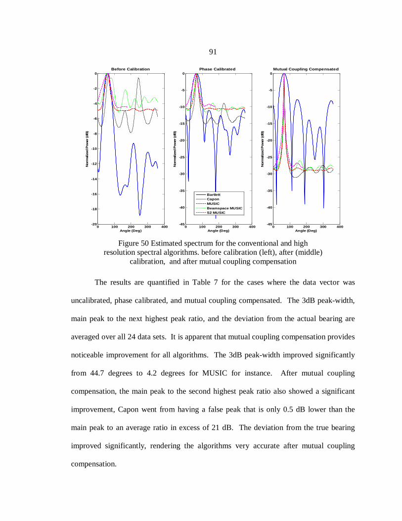
91
Figure 50 Estimated spectrum for the conventional and highresolution spectral algorithms. before calibration (left), after (middle)
calibration, and after mutual coupling compensation
The results are quantified in Table 7 for the cases where the data vector was
uncalibrated, phase calibrated, and mutual coupling compensated. The 3dB peak-width,
main peak to the next highest peak ratio, and the deviation from the actual bearing are
averaged over all 24 data sets. It is apparent that mutual coupling compensation provides
noticeable improvement for all algorithms. The 3dB peak-width improved significantly
from 44.7 degrees to 4.2 degrees for MUSIC for instance. After mutual coupling
compensation, the main peak to the second highest peak ratio also showed a significant
improvement, Capon went from having a false peak that is only 0.5 dB lower than the
main peak to an average ratio in excess of 21 dB. The deviation from the true bearing
improved significantly, rendering the algorithms very accurate after mutual coupling
compensation.
0 100 200 300 400-20
-18
-16
-14
-12
-10
-8
-6
-4
-2
0
Angle (Deg)
Nor
mal
ized
Pow
er (d
B)
Before Calibration
0 100 200 300 400-45
-40
-35
-30
-25
-20
-15
-10
-5
0
Angle (Deg)
Nor
mal
ized
Pow
er (d
B)
Phase Calibrated
0 100 200 300 400-45
-40
-35
-30
-25
-20
-15
-10
-5
0
Angle (Deg)
Nor
mal
ized
Pow
er (d
B)
Mutual Coupling Compensated
BartlettCaponMUSICBeamspace MUSICS2 MUSIC

92
Table 7 Algorithms performance averaged over the acquired data set (24 bearings)
3dB peak-width (degrees)
Main peak to the second highestratio
(mean of the highest second peak)(dB)
Deviation from true peak(degrees)
Beforecal
Aftercenter
cal
Mutualcoupling
com
Beforecal
Aftercenter
cal
Mutualcoupling
com
Beforecal
Aftercenter
cal
Mutualcoupling
com
Bartlett 44.78 43.91 43.56 6.18 9.57 7.80 11.75 0.04 0
Capon 46.09 13.04 4.26 0.43 9.50 21.36 14.00 0.04 0.04
MUSIC 44.70 19.56 4.26 4.13 9.64 23.94 11.70 0.04 0
BeamspaceMUSIC 51.22 19.04 4.52 3.06 8.89 23.20 7.50 0.79 0
S2-MUSIC 43.08 14.75 6.78 N2P N2P N2P 2.42 0.04 0.08
To demonstrate the consistency of the data depicted for a single source, 60 sets of
data were acquired to quantify how the DOA estimation varies when the same estimate is
of interest. The root mean square error (RMSE) results showed that except with Capon,
all the other algorithms showed an excellent stability in the estimate. Capon exhibited a
0.84 degree variance over the 60 runs after mutual coupling compensation (1.38 degrees
without calibration and 0.89 degrees with phase calibration).
A series of figures showing the estimated spectrum for all the algorithms of
concern at all the measured bearings for two data sets including the one used to obtain the
above results are given in Appendix B (single sources set 1). A second set of data was
processed to further verify the results and they were comparable to the one shown in this
section, the estimated spectrum for the algorithm for the second set of data is shown in
Appendix B (single sources set 2).

93
Two CW Sources Results
Two sources, one generating from the function generator (5.8 GHz) and the other
from the analog frequency synthesizer (5.7998 GHz), were used in this test (receiver
board LO was set to 5.7993 GHz). The 1st and 2nd source were at 500 KHz and 700 KHz
IF, respectively. The estimated true peaks were at bearings 10 degrees and 86 degrees.
Results for before and after calibration along with results after mutual coupling
compensation for one of the bearings are depicted in Figure 51 for Bartlett, Capon,
MUSIC, beamspace MUSIC, and S2 MUSIC. Results for the 3dB beamwidth, 3rd
highest peak, and bearing error are summarized in Table 8 when mutual coupling
compensation was applied. The results indicate that the subspace method performed
well, with a maximum 3dB beamwidth of 9 degrees (for beamspace MUSIC). The
bearing error was within one degree of error and the third highest peak was in excess of
20 dB lower than the peaks of interest. Compared to the case where only one source was
used, the 1st peak which resulted in a lower power compared to the 2nd peak had a wider
3dB beamwidth; besides the latter the bearing error and the ratio of the peak(s) to floor
were comparable. The next section investigates how the difference in power between the
1st and 2nd sources affect the DOA estimates.
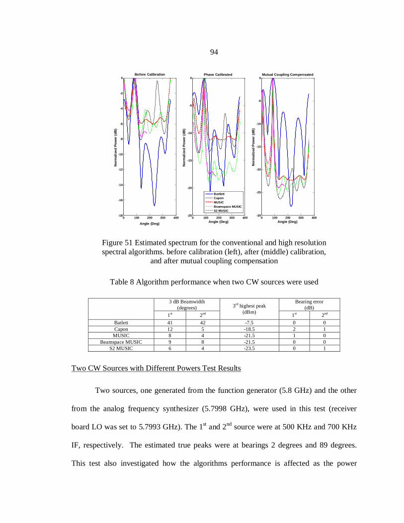
94
Figure 51 Estimated spectrum for the conventional and high resolutionspectral algorithms. before calibration (left), after (middle) calibration,
and after mutual coupling compensation
Table 8 Algorithm performance when two CW sources were used
3 dB Beamwidth(degrees) 3rd highest peak
(dBm)
Bearing error(dB)
1st 2nd 1st 2nd
Batlett 41 42 -7.5 0 0Capon 12 5 -18.5 2 1
MUSIC 8 4 -21.5 1 0Beamspace MUSIC 9 8 -21.5 0 0
S2 MUSIC 6 4 -23.5 0 1
Two CW Sources with Different Powers Test Results
Two sources, one generated from the function generator (5.8 GHz) and the other
from the analog frequency synthesizer (5.7998 GHz), were used in this test (receiver
board LO was set to 5.7993 GHz). The 1st and 2nd source were at 500 KHz and 700 KHz
IF, respectively. The estimated true peaks were at bearings 2 degrees and 89 degrees.
This test also investigated how the algorithms performance is affected as the power
0 100 200 300 400-18
-16
-14
-12
-10
-8
-6
-4
-2
0
Angle (Deg)
Nor
mal
ized
Pow
er (d
B)
Before Calibration
0 100 200 300 400-25
-20
-15
-10
-5
0
Angle (Deg)
Nor
mal
ized
Pow
er (d
B)
Phase Calibrated
0 100 200 300 400-30
-25
-20
-15
-10
-5
0
Angle (Deg)
Nor
mal
ized
Pow
er (d
B)
Mutual Coupling Compensated
BartlettCaponMUSICBeamspace MUSICS2 MUSIC

95
difference between the two sources is varied. The power in the second signal was fixed
and the first signal’s power was varied such that difference in power between the two
signals went from -10 dB to -35 dB in a 5 dB increments. Note that compared to the
previous section, the power levels used for this set up were lower. The estimated
spectrums for all varying power difference between the two signals for Bartlett, Capon,
MUSIC, beamspace MUSIC, and S2 MUSIC are depicted in Figure 52, Figure 53, Figure
54, Figure 55, and Figure 56, respectively.
The first observation applies to Bartlett. It is clear from Figure 52 that once the
power difference between the signals is lower than the sidelobe levels, the second source
cannot be detected and is considered a sidelobe. This behavior is anticipated since
Bartlett estimates are based on received power spectrum. Compared to all the remaining
algorithms Capon did poorly when the power difference was increased.
Figure 52 Estimated Spectrum for Bartlett for a varying powerdifference between the impinging sources
0 50 100 150 200 250 300 350 400-30
-25
-20
-15
-10
-5
0Bartlett- Signals power diffference and its effect on DOA estimation peaks
Angle (Deg)
Nor
mal
ized
Pow
er (d
B)
Equal power-10 dBm difference-15 dBm difference-20 dBm difference-25 dBm difference-30 dBm difference-35 dBm difference

96
Figure 53 Estimated Spectrum for Capon for a varying powerdifference between the impinging sources
Figure 54 Estimated Spectrum for MUSIC for a varying powerdifference between the impinging sources
0 50 100 150 200 250 300 350 400-25
-20
-15
-10
-5
0Capon - Signals power diffference and its effect on DOA estimation peaks
Angle (Deg)
Nor
mal
ized
Pow
er (d
B)
Equal power-10 dBm difference-15 dBm difference-20 dBm difference-25 dBm difference-30 dBm difference-35 dBm difference
0 50 100 150 200 250 300 350 400-25
-20
-15
-10
-5
0MUSIC - Signals power diffference and its effect on DOA estimation peaks
Angle (Deg)
Nor
mal
ized
Pow
er (d
B)
Equal power-10 dBm difference-15 dBm difference-20 dBm difference-25 dBm difference-30 dBm difference-35 dBm difference

97
Figure 55 Estimated Spectrum for beamspace MUSIC for a varying powerdifference between the impinging sources
Figure 56 Estimated Spectrum for S2 MUSIC for a varying powerdifference between the impinging sources
0 50 100 150 200 250 300 350 400-25
-20
-15
-10
-5
0Beamspace MUSIC - Signals power diffference and its effect on DOA estimation peaks
Angle (Deg)
Nor
mal
ized
Pow
er (d
B)
Equal power-10 dBm difference-15 dBm difference-20 dBm difference-25 dBm difference-30 dBm difference-35 dBm difference
0 20 40 60 80 100 120 140 160 180-25
-20
-15
-10
-5
0S2 MUSIC - Signals power diffference and its effect on DOA estimation peaks
Angle (Deg)
Nor
mal
ized
Pow
er (d
B)
Equal power-10 dBm difference-15 dBm difference-20 dBm difference-25 dBm difference-30 dBm difference-35 dBm difference

98
Results are summarized in Table 9 for all the algorithms after mutual coupling
compensation. The reader should note that the measurements shown are based on one set
of measurements. To verify the consistency of the estimates, 10 sets of data for the same
bearing were acquired and processed in the case were the two signals exhibited the same
power. No notable changes were noted in the spectrum of all the algorithms, except for
Capon, which showed a variation in the bearing estimate of the 1st peak of about 3
degrees along with a variation on the peak power of about 2dB. All the other algorithms
showed no sign of variation over all data sets.
The parameters of interest are the 3 dB peak-width, the resulting power of the 1st
and 2nd peaks, the 3rd highest peak and the bearing error. It is apparent that Bartlett and
Capon perform poorly when the power difference between the two sources is 10 dB or
higher. MUSIC, beamspace MUSIC and S2 MUSIC showed superb performance of
bearing error. The beam corresponding to the peak with the lower power setting showed
a significant widening. The 3rd highest peak compared to the second peak stayed about
constant after the 10 dB difference mark for all algorithms except Bartlett, where the
second peak became a mere sidelobe. Overall it was noticed that the 3dB peak-width
increased slightly when two source measurements are conducted compared to a single
source.

99
Table 9 Summary for data for all algorithms after mutual couplingcompensation for two sources with varying power difference
BartlettSig. power difference
(dB)
3 dB peak-width(degrees) Power (dBm) 3rd highest peak
(dBm)
Bearing error(degrees)
1st 2nd 1st 2nd 1st 2nd
0 46 44 0 -0.74 -5.9 0 0-10 38 42 -5.5 0 -5.5 9 2-15 34 42 -6.7 0 -6.7 12 2-20 34 42 -7.2 0 -7.2 13 2-25 34 42 -7.4 0 -7.4 13 2-30 34 42 -7.4 0 -7.4 13 2-35 34 42 -7.4 0 -7.4 13 2
CaponSig. power difference
3 dB peak-width Power3rd highest peak
Bearing error1st 2nd 1st 2nd 1st 2nd
0 14 8 -0.9 0 -10 5 0-10 42 6 -10.8 0 -19 13 1-15 42 6 -10.9 0 -18 13 1-20 40 6 -11.3 0 -19 16 1-25 45 6 -11.4 0 -18.5 16 1-30 43 6 -11.8 0 -18.4 18 1-35 58 6 -12 0 -18.2 16 1
MUSICSig. power difference
3 dB peak-width Power 3rd highest peak Bearing error
1st 2nd 1st 2nd 1st 2nd
0 10 8.5 0 -1.1 -13 1 2-10 20 8 -8.5 0 -17 1 2-15 20 7 -10.3 0 -18.4 1 2-20 20 5.5 -10.6 0 -18.9 1 2-25 20 4.5 -11.9 0 -18.9 1 2-30 60 4.4 -15.2 0 -19.8 1 2-35 90 5.5 -16.2 0 -20 1 2
Beamspace MUSICSig. power difference
3 dB peak-width Power3rd highest peak
Bearing error1st 2nd 1st 2nd 1st 2nd
0 12 10 -0.9 0 -10 2 0-10 18 3.5 -10.8 0 -19 1 1-15 20 3.5 -10.9 0 -18 1 1-20 22 2.5 -11.3 0 -19 1 1-25 28 2.5 -11.4 0 -18.6 1 1-30 24 2.5 -11.8 0 -18.4 1 1-35 24 2.5 -12 0 -18.2 2 1
S2 MUSICSig. power difference
3 dB Beamwidth Power3rd highest peak
Bearing error
1st 2nd 1st 2nd 1st 2nd
0 9 12.5 0 -3.3 -14.6 0 3-10 18 5 -8.4 0 -17.5 0 1-15 20 8 -11.3 0 -19.6 0 1-20 21 7.4 -16.1 0 -20.5 0 1-25 21 7.5 -12.1 0 -20.6 0 1-30 22 6.6 -12.5 0 -22.3 1.5 1-35 29 6.6 -14 0 -22.8 3 1
The MUSIC algorithm is given as an example in Figure 57 to show how the
algorithm behaves when phase calibration and mutual coupling compensation are applied

100
to the data vector for the varying power difference between the two sources. The spectra
for the rest of the algorithms can be found in Appendix B (Two CW signals with varying
power difference).
Figure 57 MUSIC algorithm estimated spectrum for different varyingpower difference in the uncalibrated, phase calibrated and
mutual coupling compensated case
Harris SeaLancet RT1944/U Radio Signal
The Harris SeaLancet RT1944/U Radios were used to test the capability of the
system to detect signals emitting from radios utilizing a wideband signal. Two units were
used where one was set to be the master and the other to be the slave. The SNR was set
to 25 dB and the transmit signal strength used was -10 dBm. A 50 dB attenuation was
used between the two units. The transmission speed used was 10 MBPS and the
0 200 400-15
-10
-5
0
Angle (Deg)
Nor
mal
ized
Pow
er (d
B)
Equal Power
0 200 400-20
-18
-16
-14
-12
-10
-8
-6
-4
-2
0-10 dB difference
0 200 400-20
-18
-16
-14
-12
-10
-8
-6
-4
-2
0-15 dB difference
0 200 400-25
-20
-15
-10
-5
0-20 dB difference
0 200 400-25
-20
-15
-10
-5
0-25 dB difference
0 200 400-25
-20
-15
-10
-5
0-30 dB difference
0 200 400-25
-20
-15
-10
-5
0-35 dB difference
UncalibratedPhase CalibratedMutual Coupling Compensated
MUSIC

101
occupied bandwidth of the modulated signal was 20 MHz. The estimated spatial
spectrum for all algorithms of interest are shown in Figure 58 while the 3dB beamwidth
along with the main peak to the second highest peak and deviation peak are summarized
in Table 10.
Results indicate that the accuracy of bearing estimates is very good overall
showing a maximum deviation in MUSIC with 2 degrees of error. Compared to the
results shown in Table 7, the accuracy in detecting a wideband signal source after mutual
coupling compensation is within a dB of the true peak except for MUSIC where the error
was 2 degrees. In addition, the ratio of the main peak to the second highest peaks is
higher compared to CW results, along with a noticeable widening of the 3dB beamwidth.
The first factor leading to the latter is attributable to behavior of the high resolution
algorithms, which assume a narrow band signal while the signal used here is not. In
addition, the SNR used in this case was 25dB compared to 34 dB in the CW case.
Another important factor is related to the fact that only a portion of the WiMAX signal
(5% of the overall signal is passed) is used since the maximum sampling rate allowed by
the data acquisition system is 2.5 MSPS.

102
Figure 58 Estimated Spatial spectrum for DOA estimation algorithmswhen a WiMAX signal is used. Uncalibrated (Left), Phase
Calibrated (center), and Mutual coupling Compensated (right)
Table 10 Algorithms performance when a WiMAX signal is used
3dB peak-width(Degrees)
Main peak to the second highestratio (dB)
(mean of the highest second peak)
Deviation from true peak.(Degrees)
Beforecal
Aftercenter
cal
Mutualcoupling
com
Beforecal
Aftercenter
cal
Mutualcoupling
com
Beforecal
Aftercenter
cal
Mutualcoupling
com
Bartlett 44 45 44 2.5 3.4 4.3 9 6 0
Capon 24 23.5 9.2 0 0.5 11.2 6 2 1
MUSIC 34.5 24 16 5.5 7.4 11 10 6 2
BeamspaceMUSIC 42 54 18.7 3.5 3.5 9.5 10 4 0
S2-MUSIC 31 23.5 14 6 6.5 13.5 8 7 1
0 100 200 300 400-15
-10
-5
0Uncalibrated
Angle (Deg)
Nor
mal
ized
Pow
er (d
B)
0 100 200 300 400-15
-10
-5
0Phase Calibrated
0 100 200 300 400-20
-18
-16
-14
-12
-10
-8
-6
-4
-2
0Mutual Coupling compensated
BartlettCaponMUSICBeamspace MUSICS2 MUSIC

103
Effect of Signal Frequency on the DOA Estimate
As mentioned in Chapter five, the frequency response of the filters in the 8-
channel receiver board varies from one channel to the other and above 500 KHz the
phase is not consistent. The goal in this section is to quantify how this variation of phase
over the IF band affects the estimated DOA. For the same bearing, the LO drive
frequency was varied to produce an output of 100 KHz to 1.2 MHz in 100 KHz
increments. Only the data that was mutual coupling compensated is shown in this section
and is depicted in Figure 59. Relying on phase calibration alone beyond the point of
phase consistency causes a significant deviation from the true peak, but based on the
results from mutual coupling compensated data the estimates are still accurate to within 4
degrees when the IF frequency is below the 3dB point of the filter response. At 1.2 MHz
we see that all the algorithms fail to yield accurate results and that is not only due to the
filter but also one should note that at the highest frequency, the sampling is at the Nyquist
threshold. One way to minimize the accuracy error in this case is to build a filter that
extends beyond the desired IF pass frequency but just high enough to exhibit stable phase
within the desired IF band.

104
Figure 59 Effect of IF frequency on DOA estimates
Table 11 Deviation (degrees) from actual bearing for a varying IF frequency
500KHz
600KHz
700KHz
800KHz
900KHz
1000KHz
1100KHz
1200KHz
Bartlett 1 2 4 5 1 1 4 20
Capon 1 2 4 5 1 1 4 20
MUSIC 1 1 4 1 1 1 1 4
BeamspaceMUSIC 3 4 8 1 0 0 6 23
S2 MUSIC 1 2 10 3 5 5 3 27
Close Frequency vs. Number of Samples
Since the algorithms used assume non-coherent signals, finding how spectrally
close signals affect the DOA estimates is crucial. Two CW sources were used and were
set to be 2 KHz apart. The number of samples used was also varied from 50, 100, to
1000 samples a fixed bearing. The calibrated, uncalibrated and mutual coupling
0 200 400-40
-35
-30
-25
-20
-15
-10
-5
0
Angle (Deg)
Nor
mal
ized
Pow
er (d
B)
Bartlett
0 200 400-40
-35
-30
-25
-20
-15
-10
-5
0Capon
0 200 400-16
-14
-12
-10
-8
-6
-4
-2
0MUSIC
0 200 400-18
-16
-14
-12
-10
-8
-6
-4
-2
0Beamspace MUSIC
0 200 400-16
-14
-12
-10
-8
-6
-4
-2
0S2 MUSIC
100 KHz IF500 KHz IF1 MHZ IF1.2 MHz IF
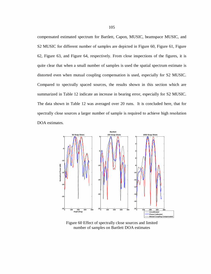
105
compensated estimated spectrum for Bartlett, Capon, MUSIC, beamspace MUSIC, and
S2 MUSIC for different number of samples are depicted in Figure 60, Figure 61, Figure
62, Figure 63, and Figure 64, respectively. From close inspections of the figures, it is
quite clear that when a small number of samples is used the spatial spectrum estimate is
distorted even when mutual coupling compensation is used, especially for S2 MUSIC.
Compared to spectrally spaced sources, the results shown in this section which are
summarized in Table 12 indicate an increase in bearing error, especially for S2 MUSIC.
The data shown in Table 12 was averaged over 20 runs. It is concluded here, that for
spectrally close sources a larger number of sample is required to achieve high resolution
DOA estimates.
Figure 60 Effect of spectrally close sources and limitednumber of samples on Bartlett DOA estimates
0 100 200 300 400-30
-25
-20
-15
-10
-5
0
Angle (Deg)
Nor
mal
ized
Pow
er (d
B)
50 Snap Shots
0 100 200 300 400-25
-20
-15
-10
-5
0100 Snap Shots
0 100 200 300 400-20
-18
-16
-14
-12
-10
-8
-6
-4
-2
01000 Snap Shots
UncalibratedPhase CalibratedMutual Coupling Compensated
Bartlett

106
Figure 61 Effect of spectrally close sources and limitednumber of samples on Capon DOA estimates
Figure 62 Effect of spectrally close sources and limitednumber of samples on MUSIC DOA estimates
0 100 200 300 400-12
-10
-8
-6
-4
-2
0
Angle (Deg)
Nor
mal
ized
Pow
er (d
B)
50 Snap Shots
0 100 200 300 400-14
-12
-10
-8
-6
-4
-2
0100 Snap Shots
0 100 200 300 400-16
-14
-12
-10
-8
-6
-4
-2
01000 Snap Shots
UncalibratedPhase CalibratedMutual Coupling Compensated
Capon
0 100 200 300 400-6
-5
-4
-3
-2
-1
0
Angle (Deg)
Nor
mal
ized
Pow
er (d
B)
50 Snap Shots
0 100 200 300 400-10
-9
-8
-7
-6
-5
-4
-3
-2
-1
0100 Snap Shots
0 100 200 300 400-15
-10
-5
01000 Snap Shots
UncalibratedPhase CalibratedMutual Coupling Compensated
MUSIC

107
Figure 63 Effect of spectrally close sources and limitednumber of samples on beamspace MUSIC DOA estimates
Figure 64 Effect of spectrally close sources and limitednumber of samples on S2 MUSIC DOA estimates
0 100 200 300 400-10
-9
-8
-7
-6
-5
-4
-3
-2
-1
0
Angle (Deg)
Nor
mal
ized
Pow
er (d
B)
50 Snap Shots
0 100 200 300 400-12
-10
-8
-6
-4
-2
0100 Snap Shots
0 100 200 300 400-18
-16
-14
-12
-10
-8
-6
-4
-2
01000 Snap Shots
UncalibratedPhase CalibratedMutual Coupling Compensated
Beamspace MUSIC
100 150 200 250 300 350-14
-12
-10
-8
-6
-4
-2
0
Angle (Deg)
Nor
mal
ized
Pow
er (d
B)
50 Snap Shots
100 150 200 250 300 350-14
-12
-10
-8
-6
-4
-2
0100 Snap Shots
100 150 200 250 300 350-20
-18
-16
-14
-12
-10
-8
-6
-4
-2
0100 Snap Shots
UncalibratedPhase CalibratedMutual Coupling Compensated
S2 MUSIC

108
Table 12 1st and 2nd peak deviation from the true bearing for a varying number of samplesused
1st Peak mean deviation (degrees) 2nd Peak mean deviation (degrees)50 100 1000 50 100 1000
Bartlett (no Cal) 30.2381 20.5714 7.5714 30.6667 21.1429 9.7143Bartlett (phase Cal) 20 13.6190 4.3810 35.4286 15.7619 5.1905Bartlett (MC comp) 62.3810 57.0476 0.9524 62.4762 56.3810 0
Capon(no Cal) 43.8095 86.5238 38.0952 45.9048 84.1429 79.0952Capon(phase Cal) 10.9524 15.1905 0.4762 119.0476 133.5714 134.4286Capon(MC comp) 43.8095 49.1429 0.3333 45.9048 56.9048 0.7143MUSIC(no Cal) 63.7619 28.0476 7.1429 64 41.8095 9.9524
MUSIC(phase Cal) 16.5714 11.6190 4.1429 30.6190 10.5714 6.5238MUSIC(MC comp) 64 47.6667 1 63.7619 47.7143 0.1905
Beamspace MUSIC(no Cal) 8.1429 92.9048 6.5714 139.5714 6.1905 24.9048Beamspace MUSIC(phase Cal) 4.9048 5.0952 2 51 25.0952 3.8571
Beamspace MUSIC 56.1905 64.0476 0.5714 57.2381 61.7143 2.0476S2 MUSIC(no Cal) 44.1429 140.9048 1.3333 134.9524 32.5238 161.7143
S2 MUSIC(phase Cal) 33.1429 139.3333 11.6667 140.5238 31.1429 151.8095S2 MUSIC(MC comp) No peak No peak 6 86.6190 86.7619 16
Summary of Results
In this Chapter the results for a variety of experiments that were carried out was
shown. Both a single and dual CW sources were tested along with a WiMAX signal.
The results show that mitigating the mutual coupling effects is imperative to achieving
high resolution performance. Compared to a single source case, when multiple sources
are used, a beam widening along with a slightly higher error in accuracy was recorded
when the two sources exhibit the same power. When the power difference is significant,
Bartlett and Capon performed poorly while the high resolution algorithms yielded superb
performance in estimating the angles of arrival.
When the Harris radios were used to test with a WiMAX signal, though the
accuracy of estimating the bearings for all the algorithms was excellent, the 3dB
beamwidth and the ratio of the main peak to the second highest peak were poorer than
when a CW signal was used. The reasons for the observed degradation are that in the
109
experiment a lower SNR was used compared to the CW case, in addition to the fact that
the signal used is not narrow band. Finally, only a portion of the available channel
bandwidth was used which means that only a fraction of the signal power is captured, this
will affects the performance of DOA estimation algorithms.
When the 1MHz channel was utilized, the IF frequency was varied to verify the
performance of the algorithms under varying IF frequency. It was concluded that with
mutual coupling compensation the algorithms performed well beyond the 3dB point of
the filters and failed to perform only when the sampling rate was at the threshold of the
Nyquist criterion. Signal coherence effects were examined by using two sources that
were set to be 2 KHz apart. It was concluded using a lower number of sample degrades
the performance of the algorithms significantly when the sources are spectrally close
(2KHz).
The above results show how well the spectral algorithms perform in a lab setting.
With the current lab setting, resolution could not be tested properly since the chamber is
not big enough to have a small angular source separation without having the two antennas
interfere with one another. Future lab equipment will allow more accurate testing
without having to approximate the angle of arrival based on a blind algorithms. Having
knowledge of the exact angle when conducting a test not only helps to provide a more
accurate metric on the algorithms performance but will enable improvement in the
calibration method.

110
CHAPTER SIX
CONCLUSION AND FUTURE WORK
The goal to equip the smart antenna system at Montana State University with a
high resolution and computationally efficient DOA estimation algorithm was met. The
challenges in implementing high resolution DOA estimation algorithms in a real system
at 5.8 GHz have been addressed in this research. Conventional and subspace based
spectral DOA estimation algorithms have been analyzed and a novel computationally
efficient alternative was presented. Though more susceptible than MUSIC to certain
parameter variations (SNR, mutual coupling…), the error in S2 MUSIC is not significant
enough to result in major accuracy or resolution degradation according to simulation
results. The major drawback of S2 MUSIC is that it can detect fewer sources then
conventional MUSIC since S2 MUSIC relies on reducing the size of the covariance
matrix.
Lab tests showed that S2 MUSIC has remarkable performance compared to
MUSIC. In addition, S2 MUSIC, due to its reduced search space, is not subject to
sidelobes which is the case for other algorithms. A significant amount of time and
effort was necessary to implement the hardware needed to achieve our goal. Phase
stability was a major concern and the hardware designed showed good phase stability
thanks to the mechanical rigidity provided by the designed enclosure. Test results
showed that the receiver board is able to successfully estimate bearings of sources that
are as low as -90 dBm. When the receiver board was subject to strong signals, the front
end saturation did not affect the DOA estimates. When multiple sources were tested, the

111
high resolution spectral algorithms showed a remarkable ability to estimate sources even
if the power difference between them is in excess of 35 dB and the maximum deviation
of 3 degrees from the actual bearing was measured when S2 MUSIC was used (power
difference between the two sources was 35dB). Over all, the accuracy of the high
resolution spectral subspace based DOA estimation algorithms was within 2 degrees of
the actual bearing.
Good hardware design was necessary but not sufficient to reach theoretical
performance; mitigating unwanted effects inherent in the hardware was necessary as well.
Calibrating for magnitude and phase errors in the system by means of current injection
improved the DOA estimates compared to the case where no calibration was applied.
The accuracy of estimation was improved significantly. Without calibration the estimates
were up to 14 degrees from the actual bearing (in the case of MUSIC). After the current
injection calibration was applied the deviation from the true peak was within a fraction of
a degree. In addition, the 3dB peak-width improved from 46 degrees to about 20 degree
after applying the current injection calibration. Mitigating the effect of mutual coupling
proved to be the key step in approaching theoretical performance. The results showed
that the 3dB peak-width went from about 45 degree to about 4 degree after applying the
new calibration method.
The offline calibration method showed very encouraging results. The method
corrects not only for mutual coupling, but also for phase differences, which eliminates the
need to perform current injection. Knowledge of the exact bearings of the sources used

112
for calibration is not required for this method, though having that information saves on
the computation burden.
To the knowledge of the author, this is the first time such performance for high
resolution DOA estimation algorithms was achieved in a real world scenario with such
promising results. Most of the work done, especially at 5.8GHz, relied on simulation
predictions and many experts in the field agreed that though theoretically subspace based
methods are superior, their predicted performance is extremely hard to achieve since they
are prone to the errors inherent in the system.
Though a significant amount of work was done to test the performance of the
system, more work remains and the following summarizes some of the key future tasks:
Test the system with a lab set up able to provide accurate bearings (this set up is
currently considered for purchase by our group). This will further validate the
results presented.
Test the system in an outdoor environment to investigate how the system will
perform outside the lab; the outdoor test will also allow for further testing of
multi-sources.
Incorporate the DOA block in the adaptive smart antenna system (this is currently
being pursued and will be achieved shortly).
Investigate alternative calibration methods or modify the current offline method to
provide the system with the ability to self-calibrate.
Future designs should consider a single board implementation for both DOA
estimation and beamforming.

113
Tracking was not considered in this work and investigating tracking algorithms is
highly desirable.

114
REFERENCES CITED

115
[1] Dr. Yikun Huang (PI), Dr. Richard S. Wolff (CO-PI) “Smart Adaptive Antennasfor Wireless Communications in Rural and Sparsely Populated Areas” proposed andaccepted by MBRCT
[2] B. Allen, M. Ghavami “Adaptive antenna systems: fundamentals andapplications” 2005, Wiley
[3] Godara, L.C. “Applications of antenna arrays to mobile communications. I.Performance improvement, feasibility, and system considerations” Proceedings of theIEEE, Vol 85 Issue 7
[4] T. S. Rappaport, “Wireless personal communications: Trends and challenges,”IEEE Antennas Propagat. Mag., vol. 33, pp. 19-29, Oct. 1991
[5] Khallaayoun, A., and Huang, Y., “Spatial Selective MUSIC for Direction ofArrival Estimation with Uniform Circular Array”, IEEE Antennas and PropagationSociety Annual Symposium, July 2007.
[6] P. Stoica and A. Nehorai, “MUSIC, Maximum Likelihood, and Cramer-Raobound”. IEEE Trans. Acoust. Speech Signal Processing 37 (1989), pp. 720–741.
[7] M. D. Panique “Design and evaluation of test bed software for a smart antennasystem supporting wireless communication in rural areas”, Master’s Thesis, MontanaState University, May, 2005
[8] B. D. V. Veen, K. M. Buckley, “Beamforming: A Versatile Approach to Spatialfiltering”, IEEE ASSP Magazine, April 1988
[9] Y. Huang R.Wolff, “A Compact Smart Antenna for WiMAX Radio”, IEEEmobile WiMAX, July 2009, Napa California
[10] Raymond J. Weber, “Development of a Cognitive Array System” , Master’sThesis, Montana State University, May, 2010
[11] Huang, Y., and Panique, M., “Performance analysis of a nullsteering algorithm,”IEEE APS International Symposium, June, 2007.
[12] C. GODARA, “Applications of Antenna Arrays to Mobile Communications, PartI: Performance Improvement, Feasibility, and System Considerations” PROCEEDINGSOF THE IEEE, VOL. 85, NO. 7, JULY 1997
[13] Constantine A.Balanis (1997), “Antenna theory”, Wiley, third edition
[14] P. Ioannides, C.A. Balanis, “Uniform circular arrays for smart antennas”Antennas and Propagation Magazine, IEEE Aug 2005, vol 47 Issue 4

116
[15] Louis L. Schart “Statistical signal processing: detection, estimation, and timeseries analysis”.Addision-Wesley Publishing company, 1991
[16] A. L. Swindlehurst and T. Kailath, “A performance analysis of subspace-basedmethods in the presence of model errors. Part I: The MUSIC algorithm,” IEEE Trans.Signal Process., vol. 40, no. 7, pp. 1758–1774, July 1992
[17] Bellini, E. and Tosi, A. “A directive system of wireless telegraphy”, 1906, Elect.Eng. 2 (11), pp. 771-775.
[18] Marconi, G. “On Methods Whereby the Radiation of Electric Waves May beMainly Confined to Certain Directions, and Whereby the Receptivity of a Receiver Maybe Restricted to Electric Waves Emanating from Certain Directions”, Proceedings of theRoyal Society of London. Series A, Containing Papers of a Mathematical and PhysicalCharacter, April 30, 1906, Vol. 77, No. 518, pp. 413-421.
[19] Adcock, F. British Patent Specification No.130490 1919.
[20] 3. Keen, R. Wireless detection finding. s.l. : Iliffe & Sons, Dorset House.
[21] Bartlett, M. S, “Periodogram Analysis and Continuous Spectra," Biometrika 37(1950), 1-16
[22] H. Krim, M. Viberg. Two decades of array signal processing research: theparametric approach . s.l. : Signal Processing Magazine, IEEE , Vol 13, Issue 4., Jul1996.
[23] Burg, J.P. , “Maximum entropy spectral analysis”, 1967, Proc. 37th annualmeeting of the society of exploration geophysicists.
[24] J. Capon “High-Resolution Frequency-Wavenumber Spectrum Analysis”PROCEEDINGS OF THE IEEE, VOL. 57, NO. 8, AUGUST 1969
[25] Borgiotti, G.V. and Kaplan, L.J. , “Superresolution of uncorrelated interferencesources by using adaptive array techniques” 1979, trans. Antennas Propag. AP-27, p. 842.
[26] Gabriel, W. , “Spectral alalysis and adaptive array superresolution thecniques”,1980, Proc. IEEE 68, p. 654.
[27] Paulraj, A ,“Subspace methods for direction of arrival”, et al. 1993, Amsterdam:North-Holland, 1993, Vol 10 Chap 16 , pp. 693-739.
[28] Pisarenko, V.F. “The retrieval of harmonics from a covariance function” 1973,Geophys.J.Roy. Astronom. Soc. 33 , pp. 347-366.

117
[29] Ralph O. Schmidt, “Multiple Emitter Location and Signal Parameter Estimation”IEEE transactions on antennas and propagation, vol. AP-34, NO.3, march 1986.
[30] Schmidt, R.O. “A signal subspace approach to multiple emitter location ofspectral estimation”, PhD Thesis, Stanford University, 1981.
[31] Bienvenu, G. and Kopp, L. , “Principe de la goniometrie passive adaptative”1979, 7° Colloque sur le traitement du signal et des images, FRA, pp. 1-10.
[32] Tufts, D.W. and Kumaresan, R. ,“Estimation of frequencies if multiple sinusoids:making linear prediction perfrom like maximum likelihood”, September 1982, Proc. ofIEEE 70, 9, pp. 975-989.
[33] Kumaresan, R. and Tufts, D.W. Estimating the angle of arrival of multiple planewaves. Jan 1983, IEEE tran. on Aerospace and Elec. Sys.AES-19 , pp. 134-139
[34] Owsley, N. L. “Signal Subspace based minimum variances spatial arrayprocessing”, November 1985, 19th Asilomar Conf., pp. 94-97.
[35] Xu, X. L. and Buckley, k. M. “A comparison of element and beamspace spatial-spectrum estimation for multiple source clusters”, April 1990, Proc. ICASSP-90 , pp.2643-2646.
[36] Paulraj, A. and Roy, R.H. , “Estimation of signal parameters via rotationalinvariance techniques-ESPRIT”, November 1985, In Proceedings of the 19tj AsilomarConference on circuits systems and Computers, pp. 83-89.
[37] Roy, R.H. “ESPRIT--Estimation of signal parameters via rotational invariancetechniques”, 1987, Ph.D dissertation, Stanford University.
[38] Kung, S. Y., Arun, K. S. and Bhashkar Roa, D.V. “New state space and singularvalue decomposition based approximation methods for harmonic retreival”, 1983, Journalof the optical society of America 73, pp. 1799-1811.
[39] Ouibrahim, H., Weiner, D. D. and Sarkar, T. K. “Matrix pencil approach to angleof arrival estimation”,November 1986, In Proceedings of the 20th Asilomar Conf. onCircuits systems and Computers, pp. 203-206.
[40] C. P. Mathews and M. D. Zoltowski, “Eigenstructure techniques for 2-d angleestimation with uniform circular arrays,” IEEE Trans. on Signal Processing, vol. 42, pp.2395-2407, Sept. 1994
[41] A.H. Tewfik, W. Hong, “ On the application of uniform linear array bearingestimation techniques to uniform circular arrays”, IEEE Trans. Signal Processing, Vol 40,pp. 1008-1011, Apr. 1992

118
[42] B. Friedlander, A. J. Weiss, “Direction finding using spatial smoothing withinterpolated arrays”, IEEE Trans. Aerosp. Electron. Syst., Vol 28, pp. 574-587, Apr. 1992
[43] Barabell, A. J. “Performance comparison of superresolution array processingalgorithms”. s.l. : Lincon Labratory, MIT, Tech. Rep. TST-72 1984.
[44] A. J. Barabell, “Improving the resolution performance of eigenstructure-baseddirection finding algorithms ” IEEE ICASSP, 1983, Boston
[45] A. N. Lemma, E. F. Deprettere, A.-J van der Veen “Experimental Analysis ofAntenna Coupling for High-Resolution DOA Estimation Algorithms” IEEE 1999

119
APPENDICES

120
APPENDIX A
HARDWARE SCHEMATICS, LAYOUT, AND BOM

121
Beamformer Board diagram
Beamformer & Antenna Array Transfer Plate
T/R Switch
T/R SwitchPA
L NA
A tten uator
5 .8 GHzWiM ax Sign al
Monopo leAnten na
Spartan 3ANFPGA
T/R Switch
T/R SwitchPA
L NA
A tten uator Monopo leAnten na
T/R Switch
T/R SwitchPA
L NA
A tten uator Monopo leAnten na
T/R Switch
T/R SwitchPA
L NA
A tten uator Monopo leAnten na
T/R Switch
T/R SwitchPA
L NA
A tten uator Monopo leAnten na
T/R Switch
T/R SwitchPA
L NA
A tten uatorMonopo leAnten na
T/R Switch
T/R SwitchPA
L NA
A tten uatorMonopo leAnten na
T/R Switch
T/R SwitchPA
L NA
A tten uatorMonopo leAnten na
8-ElementAntenna ArrayTransfer Plate
Extern alCon nection
In tern alCon nection
AmpDio de Detector
A/D
u1 x1
RSSI
WiMaxTX/RX
TX
RXTo L NAs, PAs,T/R Switches
9 6Control lin es to Attenuators
and P hase Shifters
Digital RSSI
Buffer
DC/DC LDO1.2V
3.3V
P ower to DigitalComponents
P ower toAna lo g/RF
Compo nen ts
5.1V
3.45V
Power fromModular PDS
(PowerDistribution
System) Board
Power
P hase Shifter
B and passFilter
B and passFilter
B and passFilter
B and passFilter
B and passFilter
B and passFilter
B and passFilter
B and passFilter
SurfaceTemp
Sensor2
I2C Data toSBC
Phase Shifte r
Phase Shifte r
Phase Shifte r
Phase Shifte r
Phase Shifte r
Phase Shifte r
Phase Shifte r
8-Way PowerDivider/
Combiner

122
RF Front end -1

123
RF Front end -2

124
LO drive distribution-1

125
LO drive distribution-2

126
LO drive distribution-3

127
Power Supply

128
Variable Gain amplifier-1

129
Variable Gain amplifier-2

130
Variable Gain amplifier output -1

131
Variable Gain amplifier output -2

132
IF filters-1

133
IF filters-2

134
Top Layer layout snapshot (RF layer)

135
Bottom Layer layout snapshot (IF layer)

136
Assembly Top Layer

137
Assembly Bottom Layer

138
Bill of materialItem # Quantity Part reference in schematic Part number Manifacturer Part name Part value Footprint reference
1 2 U56-57 AD8334 Analog Devices Inc IC VGA QUADW/PREAMP 64-LFCSP
LFCSP_VQ64
2 1 U55 ADF4106 analog devices frequency synthesizer TSSOP-16
3 73 C44 C49 C52 C56-64 C67 C74 C79-80 C83-90C92 C101 C103-104 C109-111 C113-116
C124 C130 C137-138 C141 C143-150 C153C162 C164-166 C169-175 C179 C186 C189C191-193 C196-197 C199-200 C202-203
C210
CAP0402 Murata ElectronicsNorth America
CAP CER .1UF 10V 10%X5R 0402
0.1µF 603
4 8 C178 C112 C142 C163 C55 C198 C91 C73 CAP0402 Panasonic - ECG CAP 18000PF 16VCERAMIC X7R 0402
0.018µF 603
5 8 C66 C188 C187 C65 C102 C97 C151-152 CAP0402 Murata ElectronicsNorth America
CAP CER 22PF 50V 5%C0G 0402
22pF 603
6 1 C105 CAP0402 Murata ElectronicsNorth America
CAP CER .1UF 10V 10%X5R 0402
0.1µF 402
7 1 C13 CAP0603 IPC SM-782 STD. SURFACE MOUNTCAPACITOR 0.031 X0.061 INCHES
.01uF 603
8 8 C43 C72 C108 C127 C129 C158 C190 C213 CAP0603 IPC SM-782 STD. SURFACE MOUNTCAPACITOR 0.031 X0.061 INCHES
??? 603
9 6 C75 C159 C180 C183 C76 C98 CAP0603 Panasonic - ECG CAP 1UF 6.3VCERAMIC X5R 0603
1.0µF 603
10 2 C117 C201 CAP0805 Murata ElectronicsNorth America
CAP CER 10UF 6.3VX5R 0805
10µF 805
11 10 C1-4 C9-12 C15 C20 CAP-CK13 KEMET AXIAL CERAMICCAPACITOR, MIL-SPECSIZE CK13
100pF 603
12 7 C7-8 C5 C17 C6 C31 C36 CAP-CK13 KEMET AXIAL CERAMICCAPACITOR, MIL-SPECSIZE CK13
0.1uF 603
13 4 C19 C32 C34 C128 CAP-CK13 KEMET AXIAL CERAMICCAPACITOR, MIL-SPECSIZE CK13
10pF 603
14 1 C23 CAP-CK13 KEMET AXIAL CERAMICCAPACITOR, MIL-SPECSIZE CK13
22uF 603
15 1 C24 CAP-CK13 KEMET AXIAL CERAMICCAPACITOR, MIL-SPECSIZE CK13
20pF 805
16 1 C25 CAP-CK13 KEMET AXIAL CERAMICCAPACITOR, MIL-SPECSIZE CK13
1.5nF 805
17 5 C26-28 C21-22 CAP-CK13 KEMET AXIAL CERAMICCAPACITOR, MIL-SPECSIZE CK13
100pF 805
18 2 C14 C16 CAP-CK13 2.2uF 80519 1 C33 CAP-CK13 KEMET AXIAL CERAMIC
CAPACITOR, MIL-SPECSIZE CK13
0.1pF 805
20 2 C29-30 CAP-CK13 KEMET AXIAL CERAMICCAPACITOR, MIL-SPECSIZE CK13
1nF 603
21 1 C18 CAP-CK13 KEMET AXIAL CERAMICCAPACITOR, MIL-SPECSIZE CK13
22uF 805
22 3 C37-39 CAP-CK13 KEMET AXIAL CERAMICCAPACITOR, MIL-SPECSIZE CK13
10uF 805
23 3 C40-42 CAP-CK13 KEMET AXIAL CERAMICCAPACITOR, MIL-SPECSIZE CK13
10.uF 805
24 16 C45 C48 C68 C71 C93 C96 C118 C121 C131C134 C154 C157 C176-177 C204 C207
CAP-CK13 KEMET AXIAL CERAMICCAPACITOR, MIL-SPECSIZE CK13
3.8nF 805
25 16 C50-51 C99-100 C122-123 C135-136 C160-161 C77-78 C184-185 C208-209
CAP-CK13 KEMET AXIAL CERAMICCAPACITOR, MIL-SPECSIZE CK13
0.38nF 805
26 1 C35 CAP-CK13 KEMET AXIAL CERAMICCAPACITOR, MIL-SPECSIZE CK13
10pF 805
27 16 C47 C132-133 C69-70 C155-156 C46 C119-120 C181-182 C95 C94 C205-206
CAP-CK13 KEMET AXIAL CERAMICCAPACITOR, MIL-SPECSIZE CK13
3.3nF 805
28 16 C107 C54 C139-140 C53 C106 C194-195 C81C167-168 C82 C125-126 C211-212
CAP-CK13 KEMET AXIAL CERAMICCAPACITOR, MIL-SPECSIZE CK13
0.33nF 805
29 4 R43 R59 R62 R78 CT-94W Copal Electronics Inc POT 10K OHM SQCERMET TOP
10.0K CT-94EW
30 1 J9 DB9-WIRE TYCO ELECTRONICS STRAIGHT DB9CONNECTOR
DB9-STRAIGHT_WIRE_M

139
31 20 FM1-20 FACTORY_MODE_0805
0805_FM
32 20 FB1-20 FERRITE_BEAD_0603
Murata FERRITE CHIP 75 OHM300MA 0603
120nH 603
33 16 L6-7 L10-11 L14-15 L18-19 L22-23 L26-27L30-31 L34-35
FERRITE_BEAD_0603
Murata FERRITE CHIP 75 OHM300MA 0603
10uH 805
34 16 L8-9 L24-25 L16-17 L28-29 L12-13 L32-33L20-21 L36-37
FERRITE_BEAD_0603
Murata FERRITE CHIP 75 OHM300MA 0603
1uH 805
35 16 U1-8 U17-24 FILTER_5515BP15C1020
panasonic bandpass filter 0805_FILTER
36 1 CLK FOX_801_TCXO
10 MHz ref clock FOX801
37 8 U33-40 GAT-ATT PL-126-ATTN38 8 U9-16 HMC318 hittite pre amp MSOP8-G39 8 U25-32 HMC488 hittite mixer MSOP8-G40 5 U45-48 U53 HMC311SC70 SC70-641 1 U54 HMC431LP4 QFN24_GND42 5 L1-5 IND-MOLDED MOLDED INDUCTOR,
0.5" PIN SPACING3.3 nH 603
43 1 D1 LED_SMT_0603
Cree Inc LED 4MM OVAL BLUE470NM
LED
44 16 F1-16 LINE_PHASE_TUNE
LITTELFUSE 345-101 FUSE HOLDER, PCBMOUNT, 1.25 X .25"FUSES
??? 0805_FM
45 3 REG1-3 LT1086-3V NATIONALSEMICONDUCTOR
5 VOLT, VOLTAGEREGULATOR
DDPAK3_LINEAR
46 1 J11 POWER_FEED_TH
GENERIC 2 PIN SIPHEADER .100 CENTERS
POWER_IN_22GUAGE
47 16 R44 R46 R48 R50 R52-53 R56 R58 R63 R65R67 R69-70 R72 R75 R77
RES0402 Vishay/Dale RES 187 OHM 1/16W1% 0402 SMD
237 603
48 2 R55 R74 RES0402 Vishay/Dale RES 10K OHM 1/16W5% 0402 SMD
10k 603
49 8 R51 R49 R71 R47 R73 R68 R54 R66 RES0402 Vishay/Dale RES 274 OHM 1/16W1% 0402 SMD
274 603
50 2 R27-28 RES0805 Yageo RES 39K OHM 1/16W5% 0402 SMD
0 805
51 4 R42 R60-61 R79 RES0805 Yageo RES 39K OHM 1/16W5% 0402 SMD
39.0K 805
52 4 R57 R64 R76 R45 RES0805 Yageo RES 39K OHM 1/16W5% 0402 SMD
0(optional) 805
53 16 R1-16 RES-WR1 IPC SM-782 STD. WIRE WOUNDRESISTOR 3.4 X 7.05MM
FS 603
54 5 R17-21 RES-WR1 IPC SM-782 STD. WIRE WOUNDRESISTOR 3.4 X 7.05MM
100 603
55 3 R22-23 R25 RES-WR1 IPC SM-782 STD. WIRE WOUNDRESISTOR 3.4 X 7.05MM
18 603
56 1 R24 RES-WR1 IPC SM-782 STD. WIRE WOUNDRESISTOR 3.4 X 7.05MM
6.2k 805
57 2 R26 R30 RES-WR1 IPC SM-782 STD. WIRE WOUNDRESISTOR 3.4 X 7.05MM
51 603
58 1 R29 RES-WR1 IPC SM-782 STD. WIRE WOUNDRESISTOR 3.4 X 7.05MM
4.3k 805
59 1 R31 RES-WR1 IPC SM-782 STD. WIRE WOUNDRESISTOR 3.4 X 7.05MM
5.1k 805
60 3 R32 R34 R37 RES-WR1 IPC SM-782 STD. WIRE WOUNDRESISTOR 3.4 X 7.05MM
10k 603
61 3 R35-36 R33 RES-WR1 IPC SM-782 STD. WIRE WOUNDRESISTOR 3.4 X 7.05MM
330 603
62 3 R38-40 RES-WR1 IPC SM-782 STD. WIRE WOUNDRESISTOR 3.4 X 7.05MM
10K 603
63 1 R41 RES-WR1 IPC SM-782 STD. WIRE WOUNDRESISTOR 3.4 X 7.05MM
270 603
64 16 J1-8 J12-18 J20 SMA_CM Amphenol Connex CONN SMA FEMALEPANEL MT 2 HOLE
SMA_CM
65 1 J19 SMA_CM Pomona SMB Connectors SMBJACK PANELRECEPTACLE
SMA_CM
66 1 S1 SW-SPST-NO C&K Components SWITCH TOGGLE SPSTSOLDER LUG
??? SPDT-CASEMT
67 8 T1-8 T1-6T DALE TA-10-08 600 - 600 OHMTELEPHONE COUPLINGAUDIO TRANSFORMER
W38_MINI_C_RF_TRANSF
68 1 J10 TEST_POINT Through Hole PC TestPoint
TEST_POINT
69 1 U52 TPS73633DBVT
SOT23-5
70 7 U41-44 U49-51 WP4F_2WAY 2way power splitter DQ1255_1

140

141

142

143

144
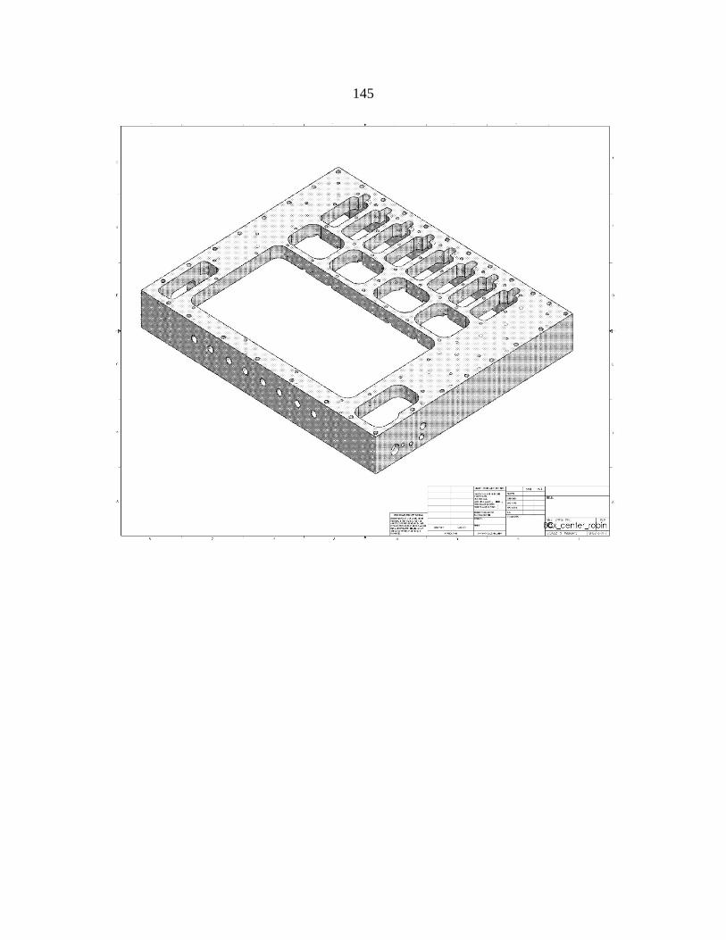
145

146

147
APPENDIX B
TEST RESULTS

148
Data set 1
Single CW Source

149
0 200 400-30
-20
-10
0
Angle (Deg)
Nor
mal
ized
Pow
er (d
B)
0 200 400-40
-30
-20
-10
0
0 200 400-30
-20
-10
0
0 200 400-25
-20
-15
-10
-5
0
Capon
0 200 400-40
-30
-20
-10
0
0 200 400-40
-30
-20
-10
0
0 200 400-30
-20
-10
0
0 200 400-25
-20
-15
-10
-5
0
0 200 400-25
-20
-15
-10
-5
0
0 200 400-25
-20
-15
-10
-5
0
0 200 400-30
-20
-10
0
0 200 400-30
-20
-10
0
0 200 400-30
-20
-10
0
0 200 400-30
-20
-10
0
0 200 400-30
-20
-10
0
0 200 400-25
-20
-15
-10
-5
0
0 200 400-25
-20
-15
-10
-5
0
0 200 400-20
-15
-10
-5
0
0 200 400-25
-20
-15
-10
-5
0
0 200 400-30
-20
-10
0
0 200 400-40
-30
-20
-10
0
0 200 400-30
-20
-10
0
0 200 400-30
-20
-10
0
0 200 400-30
-20
-10
0
No calibrationPhase calibratedMutual coupling compensated

150
0 200 400-40
-30
-20
-10
0
Angle (Deg)
Nor
mal
ized
Pow
er (d
B)
0 200 400-40
-30
-20
-10
0
0 200 400-50
-40
-30
-20
-10
0
0 200 400-40
-30
-20
-10
0
0 200 400-50
-40
-30
-20
-10
0
Bartlett
0 200 400-40
-30
-20
-10
0
0 200 400-50
-40
-30
-20
-10
0
0 200 400-50
-40
-30
-20
-10
0
0 200 400-40
-30
-20
-10
0
0 200 400-40
-30
-20
-10
0
0 200 400-40
-30
-20
-10
0
0 200 400-40
-30
-20
-10
0
0 200 400-40
-30
-20
-10
0
0 200 400-40
-30
-20
-10
0
0 200 400-50
-40
-30
-20
-10
0
0 200 400-40
-30
-20
-10
0
0 200 400-50
-40
-30
-20
-10
0
0 200 400-40
-30
-20
-10
0
0 200 400-40
-30
-20
-10
0
0 200 400-50
-40
-30
-20
-10
0
0 200 400-40
-30
-20
-10
0
0 200 400-50
-40
-30
-20
-10
0
0 200 400-40
-30
-20
-10
0
0 200 400-40
-30
-20
-10
0
No CalibrationPhase CalibratedMutual coupling compensated

151
0 200 400-25
-20
-15
-10
-5
0
Angle (Deg)
Nor
mal
ized
Pow
er(d
B)
0 200 400-30
-20
-10
0
0 200 400-30
-20
-10
0
0 200 400-20
-15
-10
-5
0MUSIC
0 200 400-30
-20
-10
0
0 200 400-40
-30
-20
-10
0
0 200 400-30
-20
-10
0
0 200 400-25
-20
-15
-10
-5
0
0 200 400-25
-20
-15
-10
-5
0
0 200 400-25
-20
-15
-10
-5
0
0 200 400-30
-20
-10
0
0 200 400-30
-20
-10
0
0 200 400-30
-20
-10
0
0 200 400-30
-20
-10
0
0 200 400-30
-20
-10
0
0 200 400-25
-20
-15
-10
-5
0
0 200 400-25
-20
-15
-10
-5
0
0 200 400-20
-15
-10
-5
0
0 200 400-25
-20
-15
-10
-5
0
0 200 400-25
-20
-15
-10
-5
0
0 200 400-40
-30
-20
-10
0
0 200 400-30
-20
-10
0
0 200 400-30
-20
-10
0
0 200 400-25
-20
-15
-10
-5
0
No CalibrationPhase CalibratedMutual Coupling Compensated

152
0 200 400-30
-20
-10
0
Angle (Deg)
Nor
mal
ized
Pow
er (d
B)
0 200 400-40
-30
-20
-10
0
0 200 400-40
-30
-20
-10
0
0 200 400-25
-20
-15
-10
-5
0
Beamspace MUSIC
0 200 400-30
-20
-10
0
0 200 400-40
-30
-20
-10
0
0 200 400-30
-20
-10
0
0 200 400-25
-20
-15
-10
-5
0
0 200 400-25
-20
-15
-10
-5
0
0 200 400-25
-20
-15
-10
-5
0
0 200 400-40
-30
-20
-10
0
0 200 400-30
-20
-10
0
0 200 400-40
-30
-20
-10
0
0 200 400-30
-20
-10
0
0 200 400-30
-20
-10
0
0 200 400-25
-20
-15
-10
-5
0
0 200 400-25
-20
-15
-10
-5
0
0 200 400-20
-15
-10
-5
0
0 200 400-30
-20
-10
0
0 200 400-25
-20
-15
-10
-5
0
0 200 400-40
-30
-20
-10
0
0 200 400-30
-20
-10
0
0 200 400-30
-20
-10
0
0 200 400-30
-20
-10
0
No CalibrationPhase CalibratedMutual Coupling Compensated

153
0 100 200-25
-20
-15
-10
-5
0
Angle (Deg)
Nor
mal
ized
Pow
er (d
B)
0 100 200-40
-30
-20
-10
0
0 100 200-30
-20
-10
0
0 100 200-20
-15
-10
-5
0S2-MUSIC
0 100 200-30
-20
-10
0
0 100 200-40
-30
-20
-10
0
0 100 200-40
-30
-20
-10
0
0 100 200-30
-20
-10
0
0 100 200-30
-20
-10
0
0 100 200-25
-20
-15
-10
-5
0
0 100 200-30
-20
-10
0
0 100 200-30
-20
-10
0
0 100 200-30
-20
-10
0
0 100 200-30
-20
-10
0
0 100 200-40
-30
-20
-10
0
0 100 200-25
-20
-15
-10
-5
0
0 100 200-25
-20
-15
-10
-5
0
0 100 200-20
-15
-10
-5
0
0 100 200-25
-20
-15
-10
-5
0
0 100 200-25
-20
-15
-10
-5
0
0 100 200-40
-30
-20
-10
0
0 100 200-25
-20
-15
-10
-5
0
0 100 200-30
-20
-10
0
0 100 200-30
-20
-10
0
No CalibratoinPhase CalibratedMutual Coupling Compensated

154
Data set 2
Single CW Source

155
0 200 400-50
-40
-30
-20
-10
0
Bartlett
Angle (Deg)
Nor
mal
ized
Pow
er (d
B)
0 200 400-50
-40
-30
-20
-10
0
0 200 400-50
-40
-30
-20
-10
0
0 200 400-50
-40
-30
-20
-10
0
0 200 400-50
-40
-30
-20
-10
0
0 200 400-50
-40
-30
-20
-10
0
0 200 400-50
-40
-30
-20
-10
0
0 200 400-50
-40
-30
-20
-10
0
0 200 400-40
-35
-30
-25
-20
-15
-10
-5
0
0 200 400-50
-40
-30
-20
-10
0
0 200 400-35
-30
-25
-20
-15
-10
-5
0
0 200 400-40
-35
-30
-25
-20
-15
-10
-5
0
UncalibratedPhase CalibratedMutual Coupling Compensated

156
0 200 400-25
-20
-15
-10
-5
0
Capon
Angle (Deg)
Nor
mal
ized
Pow
er (d
B)
0 200 400-30
-25
-20
-15
-10
-5
0
0 200 400-30
-25
-20
-15
-10
-5
0
0 200 400-30
-25
-20
-15
-10
-5
0
0 200 400-30
-25
-20
-15
-10
-5
0
0 200 400-30
-25
-20
-15
-10
-5
0
0 200 400-30
-25
-20
-15
-10
-5
0
0 200 400-30
-25
-20
-15
-10
-5
0
0 200 400-30
-25
-20
-15
-10
-5
0
0 200 400-30
-25
-20
-15
-10
-5
0
0 200 400-25
-20
-15
-10
-5
0
0 200 400-25
-20
-15
-10
-5
0
UncalibratedPhase CalibratedMutual Coupling Compensated

157
0 200 400-25
-20
-15
-10
-5
0MUSIC
Angle (Deg)
Nor
mal
ized
Pow
er (d
B)
0 200 400-30
-25
-20
-15
-10
-5
0
0 200 400-30
-25
-20
-15
-10
-5
0
0 200 400-25
-20
-15
-10
-5
0
0 200 400-30
-25
-20
-15
-10
-5
0
0 200 400-30
-25
-20
-15
-10
-5
0
0 200 400-30
-25
-20
-15
-10
-5
0
0 200 400-30
-25
-20
-15
-10
-5
0
0 200 400-25
-20
-15
-10
-5
0
0 200 400-30
-25
-20
-15
-10
-5
0
0 200 400-25
-20
-15
-10
-5
0
0 200 400-20
-15
-10
-5
0
UncalibratedPhase CalibratedMutual Coupling Compensated

158
0 200 400-25
-20
-15
-10
-5
0
Beamspace MUSIC
Angle (Deg)
Nor
mal
ized
Pow
er (d
B)
0 200 400-30
-25
-20
-15
-10
-5
0
0 200 400-30
-25
-20
-15
-10
-5
0
0 200 400-25
-20
-15
-10
-5
0
0 200 400-30
-25
-20
-15
-10
-5
0
0 200 400-35
-30
-25
-20
-15
-10
-5
0
0 200 400-30
-25
-20
-15
-10
-5
0
0 200 400-30
-25
-20
-15
-10
-5
0
0 200 400-30
-25
-20
-15
-10
-5
0
0 200 400-30
-25
-20
-15
-10
-5
0
0 200 400-30
-25
-20
-15
-10
-5
0
0 200 400-25
-20
-15
-10
-5
0
UncalibratedPhase CalibratedMutual Coupling Compensated

159
0 100 200-25
-20
-15
-10
-5
0S2 MUSIC
Angle (Deg)
Nor
mal
ized
Pow
er (d
B)
0 100 200-25
-20
-15
-10
-5
0
0 100 200-30
-25
-20
-15
-10
-5
0
0 100 200-35
-30
-25
-20
-15
-10
-5
0
0 100 200-30
-25
-20
-15
-10
-5
0
0 100 200-35
-30
-25
-20
-15
-10
-5
0
0 100 200-30
-25
-20
-15
-10
-5
0
0 100 200-30
-25
-20
-15
-10
-5
0
0 100 200-25
-20
-15
-10
-5
0
0 100 200-25
-20
-15
-10
-5
0
0 100 200-25
-20
-15
-10
-5
0
0 100 200-30
-25
-20
-15
-10
-5
0
UncalibratedPhase CalibratedMutual Coupling Compensated

160
Two CW signals with varying power difference

161
0 200 400-20
-18
-16
-14
-12
-10
-8
-6
-4
-2
0
Angle (Deg)
Nor
mal
ized
Pow
er (d
B)
Equal Power
0 200 400-25
-20
-15
-10
-5
0-10 dB difference
0 200 400-30
-25
-20
-15
-10
-5
0-15 dB difference
0 200 400-30
-25
-20
-15
-10
-5
0-20 dB difference
0 200 400-30
-25
-20
-15
-10
-5
0-25 dB difference
0 200 400-35
-30
-25
-20
-15
-10
-5
0-30 dB difference
0 200 400-35
-30
-25
-20
-15
-10
-5
0-35 dB difference
No calibrationPhase CalibratedMutual Coupling Compensated
Bartlett
0 200 400-18
-16
-14
-12
-10
-8
-6
-4
-2
0
Angle (Deg)
Nor
mal
ized
Pow
er (d
B)
Equal Power
0 200 400-25
-20
-15
-10
-5
0-10 dB difference
0 200 400-25
-20
-15
-10
-5
0-15 dB difference
0 200 400-25
-20
-15
-10
-5
0-20 dB difference
0 200 400-25
-20
-15
-10
-5
0-25 dB difference
0 200 400-25
-20
-15
-10
-5
0-30 dB difference
0 200 400-25
-20
-15
-10
-5
0-35 dB difference
UncalibratedPhase CalibratedMutual Coupling Compensated
Capon

162
0 200 400-18
-16
-14
-12
-10
-8
-6
-4
-2
0
Angle (Deg)
Nor
mal
ized
Pow
er (d
B)
Equal Power
0 200 400-25
-20
-15
-10
-5
0-10 dB difference
0 200 400-25
-20
-15
-10
-5
0-15 dB difference
0 200 400-25
-20
-15
-10
-5
0-20 dB difference
0 200 400-25
-20
-15
-10
-5
0-25 dB difference
0 200 400-25
-20
-15
-10
-5
0-30 dB difference
0 200 400-25
-20
-15
-10
-5
0-35 dB difference
UncalibratedPhase CalibratedMututal Coupling Compensated
Beamspace MUSIC
0 100 200-18
-16
-14
-12
-10
-8
-6
-4
-2
0
Angle (Deg)
Nor
mal
ized
Pow
er (d
B)
Equal Power
0 100 200-20
-18
-16
-14
-12
-10
-8
-6
-4
-2
0-10 dB difference
0 100 200-25
-20
-15
-10
-5
0-15 dB difference
0 100 200-25
-20
-15
-10
-5
0-20 dB difference
0 100 200-25
-20
-15
-10
-5
0-25 dB difference
0 100 200-25
-20
-15
-10
-5
0-30 dB difference
0 100 200-25
-20
-15
-10
-5
0-35 dB difference
UncalibratedPhase CalibratedMutual Coupling Compensated
S2 MUSIC

163
APPENDIX C
MATLAB CODE

164
Algorithms base codes
Multiple algorithms based code, including
[46] Bartlett
[47] Capon
[48] MUSIC
[49] Adapted angular response
[50] Thermal noise algorithms
[51] Maximum entropy
%%%%%%%%%%%%%%%%%%%%%%%%%%%%%%%%%%%%%%%%%%%%%%
function [P_Bar_dB,P_MEM_dB,P_AAR_dB,P_MLM_dB,P_TNA_dB,P_Music_dB_EVD] =many_alg(az1,az2,elements,power1,power2,noise,sector,samples)
Phi1 = az1; % Azimuth angled of the first incoming signalPhi2 = az2; % Azimuth angled of the second incomingsignalelements = elements; % elements in antennaant_radius = 0.3812*elements; % Antanna radiusP1 = power1; % Power of the first incoming signalP2 = power2; % power of the second incoming signalNoise_P = noise; % noise powerSector = sector; % number of sectors to scanSamPles = samples; % Number of samples
%%% constant definition
f = 5.8e9; %% operating frequencyc = 2.998e8; %% speed of lightlamda = c/f; %% operating wavelengthbeta = (2*pi)/lamda; %% wave numbereta = 120*pi;theta = pi/2; %% Elevation angle
%%% Sampling parameters
Win_per = SamPles/f;

165
T = 1/(f);Samp = floor(Win_per/T);t = linspace(0,Win_per,Samp);theta = pi/2; %% Elevation angle
%%% Sectors Spliting
k = 1:Sector;for i = 1:elements; a_t(i,:) = exp(j*ant_radius*sin(theta)*cos(k*2*(pi/Sector)-(2*(pi/elements)*i)));end
%%% Array received signals and noise
S_t1 = (P1)*(exp(j*4*pi*f*t));S_t2 = sqrt(P2)*(1+wgn(1,Samp,P2,'linear','complex'));NoiSe = wgn(elements,Samp,Noise_P,'linear','complex');x_t = a_t(:,Phi1)*S_t1 +a_t(:,Phi2)*S_t2 + NoiSe ;Rxx = x_t*ctranspose(x_t)/Samp;
%%% Beam scan algorithm
P_Barlett = ctranspose(a_t)*Rxx*a_t;P_barlett_spectrum = diag(P_Barlett);P_Bar_norm = P_barlett_spectrum/max(P_barlett_spectrum);P_Bar_dB = 10*log10(abs(P_Bar_norm));
%%% maximum entropy
iden = eye(elements,elements);
P_MEM =1./(ctranspose(a_t)*inv(Rxx)*iden(1,:)'*ctranspose(iden(1,:)')*ctranspose(inv(Rxx))*a_t);P_MEM_spec = diag (P_MEM);P_MEM_norm = P_MEM_spec/max(P_MEM_spec);P_MEM_dB = 10*log10(abs(P_MEM_norm));
%%% Adapted angular response
P_AAR = ctranspose(a_t)*inv(Rxx)*a_t./(ctranspose(a_t)*inv(Rxx^2)*a_t);P_AAR_spec = diag (P_AAR);P_AAR_norm = P_AAR_spec/max(P_AAR_spec);

166
P_AAR_dB = 10*log10(abs(P_AAR_norm));
%%% Maximum likelihood (capon)
P_MLM = 1./(ctranspose(a_t)*inv(Rxx)*a_t);P_MLM_spec = diag (P_MLM);P_MLM_norm = P_MLM_spec/max(P_MLM_spec);P_MLM_dB = 10*log10(abs(P_MLM_norm));
%%% thermal noise algorithm
P_TNA = 1./(ctranspose(a_t)*inv(Rxx^2)*a_t);P_TNA_spec = diag (P_TNA);P_TNA_norm = P_TNA_spec/max(P_TNA_spec);P_TNA_dB = 10*log10(abs(P_TNA_norm));
%%% Multiple signal classification
[eig_VEC,diag_vec] = eig(Rxx);[eigvals,ix] = sort(diag(diag_vec),'descend');eig_VEC = eig_VEC(:,ix);En = eig_VEC(:,3:elements);P_Music =1./(ctranspose(a_t)*eig_VEC(:,3:elements)*ctranspose(eig_VEC(:,3:elements))*a_t);P_Music_spectrum = diag(P_Music);P_Music_norm = P_Music_spectrum/max(P_Music_spectrum);P_Music_dB_EVD= 10*log10(abs(P_Music_norm));
figureplot(P_Bar_dB)hold onplot(P_MEM_dB,'r')plot(P_AAR_dB,'g')plot(P_MLM_dB,'k')plot(P_TNA_dB,'r:')plot(P_Music_dB_EVD,'y')
%%%%%%%%%%%%%%%%%%%%%%%%%%%%%%%%%%%%%%%%%%%%%%Beamspace%%%%%%%%%%%%%%%%%%%%%%%%%%%%%%%%%%%%%%%%%%%%%%
function [P_Music_beam_dB] =beamspace_MUSIC(Phi1,Phi2,elements,P1,P2,Noise,Sector,Points,Modes)
Phi1 = Phi1; % Azimuth angled of the first incoming signal

167
Phi2 = Phi2; % Azimuth angled of the second incomingsignalelements = elements; % elements in antennaant_radius = 0.3812*elements; %ant_radius;% 3; % Antanna radiusP1 = 10^(P1/10); % Power of the first incoming signalP2 = 10^(P2/10); % power of the second incoming signalNoise_P = 10^(Noise/10); % noise powerSector = Sector; % number of sectors to scanSamPles = Points; % Number of samplesif Phi1 == 0 Phi1 = 360;end
if Phi2 == 0 Phi2 = 360;end
%%% constant definition
f = 5.8e9; %% operating frequencyc = 2.998e8; %% speed of lightlamda = c/f; %% operating wavelengthbeta = (2*pi)/lamda; %% wave numbereta = 120*pi;theta = pi/2; %% Elevation angle
%%% Sampling parameters
Win_per = SamPles/f;T = 1/(f);Samp = floor(Win_per/T);t = linspace(0,Win_per,Samp);theta = pi/2; %% Elevation angle%%% Sectors Spliting
k = 1:Sector;for i = 1:elements; a_t(i,:) = exp(1i*ant_radius*sin(theta)*cos(k*2*(pi/Sector)-(2*(pi/elements)*i)));end
%%% Array received signals and noise
S_t1 = (P1)*(exp(j*4*pi*f*t));S_t2 = sqrt(P2)*(1+wgn(1,Samp,P2,'linear','complex'));NoiSe = wgn(elements,Samp,Noise_P,'linear','complex');x_t = a_t(:,Phi1)*S_t1 +a_t(:,Phi2)*S_t2 + NoiSe ;

168
Rxx = x_t*ctranspose(x_t)/Samp;
%%% beamspace real MUSIC for UCA
%%% define the weight vectorn = 1:1:elements;sy = (2*pi*n)/elements;Modes = Modes;
%%% generating the mode vectorM1 = -Modes:1:0;M2 = -1:-1:-Modes;MM = cat(2,M1,M2);
%%% Weight vectorCv = diag(1i.^(MM));vec_count = 0;for i = -Modes:1:Modesvec_count = vec_count+1; V(:,vec_count) =sqrt(elements)*(1/elements)*exp(1i*i*sy)';end
Feh = Cv*V';
%%% genetating the Beamspace manifold
a_bs = Feh*a_t;
%%% one can also generetate a_bs by using bessel function as follows:
ModeSS = Modes:1:Modes;bess = diag(besselj(ModeSS,ant_radius));vec_count = 0;kk = 1:Sector;for i = -Modes:1:Modes; vec_count = vec_count+1; v_phi(vec_count,:) =sqrt(elements)*exp(1i*ant_radius*sin(theta)*cos(k*2*(pi/Sector)-(2*(pi/elements)*i)));end
%%% getting W that has centro hermitian rowsM_prim = 2*Modes +1;ss = -Modes:1:Modes;

169
max_beam_num = 2*Modes+1;beam_num = 1:1:max_beam_num;W_ch = (1/sqrt(M_prim))*exp(-1i*ss'*beam_num);
Frh = W_ch'*Feh;b_theta = Frh*a_t;
y_t = Frh*x_t;Ryy = y_t*ctranspose(y_t);Ryy_real = real(Ryy);
[eig_VEC_beam,diag_vec_beam] = eig(Ryy_real);[eigvals_beam,ix_beam] = sort(diag(diag_vec_beam),'descend');eig_VEC_beam = eig_VEC_beam(:,ix_beam);En_beam = eig_VEC_beam(:,3:max_beam_num);P_Music_beam = 1./(ctranspose(b_theta)*En_beam*ctranspose(En_beam)*b_theta);P_Music_spectrum_beam = diag(P_Music_beam);P_Music_norm_beam = P_Music_spectrum_beam/max(P_Music_spectrum_beam);P_Music_beam_dB = 10*log10(P_Music_norm_beam);
%%%%%%%%%%%%%%%%%%%%%%%%%%%%%%%%%%%%%%%%%%%%%%
Spatial Selective MUSIC base algorithm%%%%%%%%%%%%%%%%%%%%%%%%%%%%%%%%%%%%%%%%%%%%%%
function [angle_music1,angle_music2,angle_s2_music1, angle_s2_music2] =S2MUSIC_two_sig(angle1,angle2,elements,P1,P2,Noise,points,var_elem,bb,bbb)
% clear all
format long
Phi1 = angle1*10; % Azimuth angled of the first incoming signalPhi2 = angle2*10; % Azimuth angled of the second incoming signal
if Phi1 == 0 Phi1 = 3600;end
if Phi2 == 0 Phi2 = 3600;end

170
ant_radius = 0.3812*elements; % Antanna radiusP1 = 10^(P1/10); % Power of the first incoming signalP2 = 10^(P2/10); % power of the second incoming signalNoise_P = 10^(Noise/10); % noise powerSector = 3600; % number of sectors to scanSamPles = points; % Number of samples
%%% constant definition
f = 5.8e9; %% operating frequencyc = 2.998e8; %% speed of light
%%% Sampling parameters
Win_per = SamPles/f;T = 1/(f);Samp = floor(Win_per/T);t = linspace(0,Win_per,Samp);theta = pi/2; %% Elevation angle%%% Sectors Spliting
k = 1:Sector;for i = 1:elements; a_t2(i,:) = exp(j*ant_radius*sin(theta)*cos(k*2*(pi/Sector)-(2*(pi/elements)*i)));end
%%% Array received signals and noise
S_t1 = (P1)*(exp(j*4*pi*f*t));S_t2 = sqrt(P2)*(1+wgn(1,Samp,P2,'linear','complex'));NoiSe = wgn(elements,Samp,Noise_P,'linear','complex');x_t = a_t(:,Phi1)*S_t1 + NoiSe + a_t(:,Phi2)*S_t2;
var_elem = 5;
if var_elem == 3if locs_1(1)>=1 && locs_1(1)<=90
shift_S2 = 0; x_t1 = x_t(1:3,:); Rxx1 = 1/size(x_t1,2) *x_t1 * x_t1'; a_t_s2 = a_t2(1:3,1:90); a_t_s2_corr = a_s2_corr1(1:3,1:90);
elseif locs_1(1)>=91 && locs_1(1)<=180 shift_S2 = 90; x_t1 = x_t(3:5,:); Rxx1 = 1/size(x_t1,2) *x_t1 * x_t1';

171
a_t_s2 = a_t2(3:5,91:180); a_t_s2_corr = a_s2_corr1(3:5,91:180);
elseif locs_1(1)>=181 && locs_1(1)<=240 shift_S2 = 180; x_t1 = x_t(5:7,:); Rxx1 = 1/size(x_t1,2) *x_t1 * x_t1'; a_t_s2 = a_t2(5:7,181:270); a_t_s2_corr = a_s2_corr1(1:3,181:270);%91:180);
elseif locs_1(1)>=241 && locs_1(1)<=360 shift_S2 = 240; x1 = x_t(6:8,:); Rxx1 = 1/size(x_t1,2) *x_t1 * x_t1'; a_t_s2 = a_t2(6:8,271:360); a_t_s2_corr = a_s2_corr1(6:8,271:360);
end
elseif var_elem == 4if locs_1(1)>=1 && locs_1(1)<=120
shift_S2 = 0; x_t1 = x_t(1:4,:); Rxx1 = 1/size(x_t1,2) *x_t1 * x_t1'; a_t_s2 = a_t2(1:4,1:120); a_t_s2_corr = a_s2_corr1(1:4,1:120);
elseif locs_1(1)>=121 && locs_1(1)<=240 shift_S2 = 120; x_t1 = x_t(4:7,:); Rxx1 = 1/size(x_t1,2) *x_t1 * x_t1'; a_t_s2 = a_t2(4:7,121:240); a_t_s2_corr = a_s2_corr1(4:7,121:240);
elseif locs_1(1)>=241 && locs_1(1)<=360 shift_S2 = 240; x_t1 = x_t(5:8,:); Rxx1 = 1/size(x_t1,2) *x_t1 * x_t1'; a_t_s2 = a_t2(5:8,241:360); a_t_s2_corr = a_s2_corr1(5:8,241:360);
endelseif var_elem == 5
if locs_1(1)>=1 && locs_1(1)<=180 shift_S2 = 0; x_t1 = x_t(1:5,:); Rxx1 = 1/size(x_t1,2) *x_t1 * x_t1'; a_t_s2 = a_t2(1:5,1:180); a_t_s2_corr = a_s2_corr1(1:5,1:180);
elseif locs_1(1)>=181 && locs_1(1)<=360 shift_S2 = 180; x_t1 = x_t(4:8,:); Rxx1 = 1/size(x_t1,2) *x_t1 * x_t1'; a_t_s2 = a_t2(4:8,181:360); a_t_s2_corr = a_s2_corr1(4:8,181:360);
endend

172
%%% S2 MUSIC spetrum generation
[eig_VEC1,diag_vec1] = eig(Rxx1);[eigvals1,ix1] = sort(diag(diag_vec1),'descend');eig_VEC1 = eig_VEC1(:,ix1);En1 = eig_VEC1(:,2:length(Rxx1));
P_S2_Music = 1./(ctranspose(a_t_s2)*En1*ctranspose(En1)*a_t_s2);P_S2_Music_spectrum = diag(P_S2_Music);P_S2_Music_norm = P_S2_Music_spectrum/max(P_S2_Music_spectrum);P_S2_Music_dB = 10*log10(abs(P_S2_Music_norm));
figuretitle('S2-MUSIC')subplot(2,9,loop-18)x_ax = linspace(1,180,180);plot(x_ax+shift_S2,P_S2_Music_dB);
%%%%%%%%%%%%%%%%%%%%%%%%%%%%%%%%%%%%%%%%%%%%%%
Element spacing varying code example%%%%%%%%%%%%%%%%%%%%%%%%%%%%%%%%%%%%%%%%%%%%%%
%%%% fixed SNR = 10%%% var element spacing
for xx = 1:200
[P_Bar_dB,P_cap_dB,P_Music_dB,P_S2_Music_dB] =S2MUSIC(45,8,10,0,1000,5,1,1,0.1); P_Bar_dB_p1(:,xx) = P_Bar_dB; P_cap_dB_p1(:,xx) = P_cap_dB; P_Music_dB_p1(:,xx) = P_Music_dB; P_S2_Music_dB_p1(:,xx) = P_S2_Music_dB;

173
endsave('lamda_var_p1','P_Bar_dB_p1','P_cap_dB_p1','P_Music_dB_p1','P_S2_Music_dB_p1')
%% note that the above loop is repeated for varying elements spacing which isthe last variable in the function’s parameter
%%%%%%%%%%%%%%%%%%%%%%%%%%%%%%%%%%%%%%%%%%%%%%%%%%%%%%%%%%%%%%%%%%%%%%%%%%
%%% Beamspace
for xx = 1:200 P_Music_beam_dB = beamspace_singlesource(45,8,10,0,3600,1000,7,0.1); P_Beam_p1(:,xx) = P_Music_beam_dB;endsave('lamda_var_beam_p1', 'P_Beam_p1')clear all
Processing example%%%%%%%%%%%%%%%%%%%%%%%%%%%%%%%%%%%%%%%%%%%%%%
clear allload lamda_var_p1load lamda_var_beam_p1for i = 1:200 [x_bar,locs_bar] =findpeaks(real(P_Bar_dB_p1(:,i)),'sortstr','descend'); [x_cap,locs_cap] =findpeaks(real(P_cap_dB_p1(:,i)),'sortstr','descend'); [x_music,locs_music]=findpeaks(real(P_Music_dB_p1(:,i)),'sortstr','descend'); [x_s2,locs_s2]=findpeaks(real(P_S2_Music_dB_p1(:,i)),'sortstr','descend'); [x_beam,locs_beam] =findpeaks(real(P_Beam_p1(:,i)),'sortstr','descend'); bar(i) = locs_bar(1); cap(i) = locs_cap(1); music(i) = locs_music(1); s2(i) = locs_s2(1); beam(i) = locs_beam(1);endMSE_bar_p1 = sqrt(sum(abs(bar-450))/200);MSE_cap_p1 = sqrt(sum(abs(cap-450))/200);MSE_music_p1 = sqrt(sum(abs(music-450))/200);MSE_s2_p1 = sqrt(sum(abs(s2-450))/200);MSE_beam_p1 = sqrt(sum(abs(beam-450))/200);
save('MSE_p1','MSE_bar_p1','MSE_cap_p1','MSE_music_p1','MSE_s2_p1','MSE_beam_p1')

174
%%% on a different m file the saved variables are loaded and organized forplotting
factor = [0.1 0.2 0.3 0.4 0.5 0.6 0.7 0.8 0.9 1 1.1 1.2 1.3 1.4 1.5 ];
MSE_all_bar = [MSE_bar_p1 MSE_bar_p2 MSE_bar_p3 MSE_bar_p4 MSE_bar_p5MSE_bar_p6 MSE_bar_p7 MSE_bar_p8 MSE_bar_p9 ... MSE_bar_1 MSE_bar_1p1 MSE_bar_1p2 MSE_bar_1p3 MSE_bar_1p4 MSE_bar_1p5];MSE_all_cap = [MSE_cap_p1 MSE_cap_p2 MSE_cap_p3 MSE_cap_p4 MSE_cap_p5MSE_cap_p6 MSE_cap_p7 MSE_cap_p8 MSE_cap_p9 ... MSE_cap_1 MSE_cap_1p1 MSE_cap_1p2 MSE_cap_1p3 MSE_cap_1p4 MSE_cap_1p5];MSE_all_music = [MSE_music_p1 MSE_music_p2 MSE_music_p3 MSE_music_p4MSE_music_p5 MSE_music_p6 MSE_music_p7 MSE_music_p8 MSE_music_p9 ... MSE_music_1 MSE_music_1p1 MSE_music_1p2 MSE_music_1p3 MSE_music_1p4MSE_music_1p5];MSE_all_s2 = [MSE_s2_p1 MSE_s2_p2 MSE_s2_p3 MSE_s2_p4 MSE_s2_p5 MSE_s2_p6MSE_s2_p7 MSE_s2_p8 MSE_s2_p9 ... MSE_s2_1 MSE_s2_1p1 MSE_s2_1p2 MSE_s2_1p3 MSE_s2_1p4 MSE_s2_1p5];MSE_all_beam = [MSE_beam_p1 MSE_beam_p2 MSE_beam_p3 MSE_beam_p4 MSE_beam_p5MSE_beam_p6 MSE_beam_p7 MSE_beam_p8 MSE_beam_p9 ... MSE_beam_1 MSE_beam_1p1 MSE_beam_1p2 MSE_beam_1p3 MSE_beam_1p4MSE_beam_1p5];
figure
plot(factor,MSE_all_bar/10,':*')hold onplot(factor,MSE_all_cap/10,'r')plot(factor,MSE_all_music/10,'k')plot(factor,MSE_all_s2/10,'g:')plot(factor,MSE_all_beam/10,'m')plot(0.37*ones(1,length(factor)),linspace(0,0.14,length(factor)),':')legend('Bartlett','Maximum likelihood','MUSIC','S2 MUSIC','Beamspace MUSIC')xlabel('Element spacing factor (Lamda)')ylabel('RMSE (deg)')
%%%%%%%%%%%%%%%%%%%%%%%%%%%%%%%%%%%%%%%%%%%%%%
Example code for resolution as the number of sampling is the variable, here the number ofsamples used is 100 and is highlighted, “hist” and “imagesc” were used to plot the results forbetter visualization of simualation results.

175
%%%%%%%%%%%%%%%%%%%%%%%%%%%%%%%%%%%%%%%%%%%%%%
%function [P_Bar_dB,P_cap_dB,P_Music_dB,P_S2_Music_dB,P_Music_beam_dB] =%S2MUSIC_two_sig(angle1,angle2,elements,P1,P2,Noise,sect,points,var_elem,bb,b%bb,del_f,Modes)
clear all
for i = 1:360
[P_Bar_dB,P_cap_dB,P_Music_dB,P_S2_Music_dB,P_Music_beam_dB] =S2MUSIC_two_sig(180,i,8,20,20,0,360,100,5,1,1,10e6,7);
P_Bar_dB_10(:,i) = P_Bar_dB;P_cap_dB_10(:,i) = P_cap_dB;P_Music_dB_10(:,i)= P_Music_dB;P_S2_Music_dB_10(:,i) = P_S2_Music_dB;P_Music_beam_dB_10(:,i) = P_Music_beam_dB;
end
save('res_samp_10','P_Bar_dB_10','P_cap_dB_10','P_Music_dB_10','P_S2_Music_dB_10','P_Music_beam_dB_10')%%%% Bartlettfor i = 1:360 [x_bar,locs_bar]=findpeaks(real(P_Bar_dB_10(:,i)),'sortstr','descend','minpeakheight',-25);
for h = 1:length(locs_bar) locs_Bar(i,h) = locs_bar(h); x_Bar(i,h) = x_bar(h);
endif length(locs_Bar) > 1
if i < 180if locs_Bar(i,1)>locs_Bar(i,2)
switCH1 = locs_Bar(i,2); switCH2 = x_Bar(i,2); locs_Bar(i,2) = locs_Bar(i,1); locs_Bar(i,1) = switCH1; x_Bar(i,2) = x_Bar(i,1); x_Bar(i,1) = switCH2;
endif i > 180
if locs_Bar(i,1)<locs_Bar(i,2) switCH1 = locs_Bar(i,2); switCH2 = x_Bar(i,2);
176
locs_Bar(i,2) = locs_Bar(i,1); locs_Bar(i,1) = switCH1; x_Bar(i,2) = x_Bar(i,1); x_Bar(i,1) = switCH2;
endendendend
end%%%% MLfor i = 1:360 [x_cap,locs_cap]=findpeaks(real(P_cap_dB_10(:,i)),'sortstr','descend','minpeakheight',-25);
for h = 1:length(locs_cap) locs_Cap(i,h) = locs_cap(h); x_Cap(i,h) = x_cap(h);
endif length(locs_Cap) > 1
if i < 180if locs_Cap(i,1)>locs_Cap(i,2)
switCH1 = locs_Cap(i,2); switCH2 = x_Cap(i,2); locs_Cap(i,2) = locs_Cap(i,1); locs_Cap(i,1) = switCH1; x_Cap(i,2) = x_Cap(i,1); x_Cap(i,1) = switCH2;
endif i > 180
if locs_Cap(i,1)<locs_Cap(i,2) switCH1 = locs_Cap(i,2); switCH2 = x_Cap(i,2); locs_Cap(i,2) = locs_Cap(i,1); locs_Cap(i,1) = switCH1; x_Cap(i,2) = x_Cap(i,1); x_Cap(i,1) = switCH2;
endendendend
end
%%%% MUSICfor i = 1:360 [x_music,locs_music]=findpeaks(real(P_Music_dB_10(:,i)),'sortstr','descend','minpeakheight',-25);
for h = 1:length(locs_music) locs_Music(i,h) = locs_music(h); x_Music(i,h) = x_music(h);
endif length(locs_Music) > 1

177
if i < 180if locs_Music(i,1)>locs_Music(i,2)
switCH1 = locs_Music(i,2); switCH2 = x_Music(i,2); locs_Music(i,2) = locs_Music(i,1); locs_Music(i,1) = switCH1; x_Music(i,2) = x_Music(i,1); x_Music(i,1) = switCH2;
endif i > 180
if locs_Music(i,1)<locs_Music(i,2) switCH1 = locs_Music(i,2); switCH2 = x_Music(i,2); locs_Music(i,2) = locs_Music(i,1); locs_Music(i,1) = switCH1; x_Music(i,2) = x_Music(i,1); x_Music(i,1) = switCH2;
endendendend
end%%%%% Beam
for i = 1:360 [x_beam,locs_beam]=findpeaks(real(P_Music_beam_dB_10(:,i)),'sortstr','descend','minpeakheight',-25);
for h = 1:length(locs_beam) locs_Beam(i,h) = locs_beam(h); x_Beam(i,h) = x_beam(h);
endif length(locs_Beam) > 1
if i < 180if locs_Beam(i,1)>locs_Beam(i,2)
switCH1 = locs_Beam(i,2); switCH2 = x_Beam(i,2); locs_Beam(i,2) = locs_Beam(i,1); locs_Beam(i,1) = switCH1; x_Beam(i,2) = x_Beam(i,1); x_Beam(i,1) = switCH2;
endif i > 180
if locs_Beam(i,1)<locs_Beam(i,2) switCH1 = locs_Beam(i,2); switCH2 = x_Beam(i,2); locs_Beam(i,2) = locs_Beam(i,1);

178
locs_Beam(i,1) = switCH1; x_Beam(i,2) = x_Beam(i,1); x_Beam(i,1) = switCH2;
endendendend
end
%%%% S2
for i = 1:225 [x_s2,locs_s2]=findpeaks(real(P_S2_Music_dB_10(:,i)),'sortstr','descend','minpeakheight',-25);
for h = 1:length(locs_s2) locs_S2(i,h) = locs_s2(h); x_S2(i,h) = x_s2(h);
endif length(locs_S2) > 1
if i < 180if locs_S2(i,1)>locs_S2(i,2)
switCH1 = locs_S2(i,2); switCH2 = x_S2(i,2); locs_S2(i,2) = locs_S2(i,1); locs_S2(i,1) = switCH1; x_S2(i,2) = x_S2(i,1); x_S2(i,1) = switCH2;
endif i > 180
if locs_S2(i,1)<locs_S2(i,2) switCH1 = locs_S2(i,2); switCH2 = x_S2(i,2); locs_S2(i,2) = locs_S2(i,1); locs_S2(i,1) = switCH1; x_S2(i,2) = x_S2(i,1); x_S2(i,1) = switCH2;
endendendend
end
histbar = hist(locs_Bar.',[1:360]);histcap = hist(locs_Cap.',[1:360]);histmusic = hist(locs_Music.',[1:360]);histbeam = hist(locs_Beam.',[1:360]);hists2 = hist(locs_S2.',[1:225]);

179
figure% axes('FontWeight','bold','FontSize',14)subplot(3,2,1)imagesc(histbar.',[0,10]);title('Bartlett Histogram','FontSize',14,'FontWeight','bold')ylabel('Set Angle [deg]','FontSize',14,'FontWeight','bold')xlabel('Detected Angle [deg]','FontSize',14,'FontWeight','bold')subplot(3,2,2)imagesc(histcap.',[0,10]);title('ML Histogram','FontSize',14,'FontWeight','bold')ylabel('Set Angle [deg]','FontSize',14,'FontWeight','bold')xlabel('Detected Angle [deg]','FontSize',14,'FontWeight','bold')subplot(3,2,3)imagesc(histmusic.',[0,10]);title('MUSIC Histogram','FontSize',14,'FontWeight','bold')ylabel('Set Angle [deg]','FontSize',14,'FontWeight','bold')xlabel('Detected Angle [deg]','FontSize',14,'FontWeight','bold')subplot(3,2,4)imagesc(histbeam.',[0,10]);title('Beamspace MUSIC Histogram','FontSize',14,'FontWeight','bold')ylabel('Set Angle [deg]','FontSize',14,'FontWeight','bold')xlabel('Detected Angle [deg]','FontSize',14,'FontWeight','bold')subplot(3,2,5)imagesc(hists2.',[0,10]);title('S2 MUSIC Histogram','FontSize',14,'FontWeight','bold')ylabel('Set Angle [deg]','FontSize',14,'FontWeight','bold')xlabel('Detected Angle [deg]','FontSize',14,'FontWeight','bold')
cm = colormap(jet);cm(1,:)=[1,1,1];colormap(cm)
%%%%%%%%%%%%%%%%%%%%%%%%%%%%%%%%%%%%%%%%%%%%%%