Received: 20 June 2016 Revised: 31 October 2016 Accepted: 28 December 2016

DOI: 10.1002/cnm.2863

R E S E A R C H A R T I C L E

High-resolution data assimilation of cardiac mechanics applied toa dyssynchronous ventricle

Gabriel Balaban1,2,5 Henrik Finsberg1,2,5 Hans Henrik Odland4,7 Marie E. Rognes1,3

Stian Ross4,5 Joakim Sundnes1,2,5 Samuel Wall1,5,6

1Simula Research Laboratory, P.O. Box 134 1325Lysaker Norway2Department of Informatics, University of Oslo,P.O. Box 1080, Blindern 0316 Oslo Norway3Department of Mathematics, University of Oslo,P.O Box 1053, Blindern 0316 Oslo Norway4Faculty of Medicine, University of Oslo, P.O. Box1078 Blindern, 0316 Oslo Norway5Center for Cardiological Innovation,Songsvannsveien 9, 0372 Oslo Norway6Department of Mathematical Science andTechnology, Norwegian University of LifeSciences, Universitetstunet 3 1430 Ås Norway7Department of Pediatrics, Oslo UniversityHospital, PO Nydalen Oslo, Norway

CorrespondenceGabriel Balaban, Simula Research Laboratory,P.O. Box 134 1325 Lysaker, Norway.Email: gabrib@math.uio.no

Funding informationResearch Council of Norway; Center forBiomedical Computing at Simula ResearchLaboratory , Grant/Award Number: 179578; Centerfor Cardiological Innovation at Oslo UniversityHospital , Grant/Award Number: 203489

AbstractComputational models of cardiac mechanics, personalized to a patient, offer accessto mechanical information above and beyond direct medical imaging. Addition-ally, such models can be used to optimize and plan therapies in-silico, therebyreducing risks and improving patient outcome. Model personalization has tradi-tionally been achieved by data assimilation, which is the tuning or optimizationof model parameters to match patient observations. Current data assimilation pro-cedures for cardiac mechanics are limited in their ability to efficiently handlehigh-dimensional parameters. This restricts parameter spatial resolution, and therebythe ability of a personalized model to account for heterogeneities that are oftenpresent in a diseased or injured heart. In this paper, we address this limitationby proposing an adjoint gradient–based data assimilation method that can effi-ciently handle high-dimensional parameters. We test this procedure on a syntheticdata set and provide a clinical example with a dyssynchronous left ventricle withhighly irregular motion. Our results show that the method efficiently handles ahigh-dimensional optimization parameter and produces an excellent agreement forpersonalized models to both synthetic and clinical data.

KEYWORDS

adjoint, cardiac mechanics, data assimilation, dyssynchrony, patient specific

1 INTRODUCTION

Computational models of cardiac mechanics, personalizedto the level of the individual through the use of clini-cal imaging, have potential to be a powerful aid in thediagnosis and treatment of cardiac disease. By relatingimage-based data to fundamental physical processes, modelscan give additional insight into the function or dysfunctionof the individual’s heart, beyond what can be directly mea-sured or observed in the images. This is becoming moreimportant as the resolution and accuracy of clinical imag-ing continues to improve. This increasingly detailed datacombined with biophysical models have promise in anal-ysis of regionally and temporally resolved differences inthe mechanics of the heart, important in diseases such asheart failure and the application of cardiac resynchronizationtherapy.

A key step in making these clinically useful cardiacmechanics models is proper data assimilation from patientobservations into a fit model. This involves the optimiza-tion, or tuning, of individual model parameters to make themodel match the observations of the patient’s heart. Overthe last decade several data assimilation methods have beendeveloped and proposed for this problem. The earliest studiesused gradient-based optimization to minimize the discrep-ancy between model-derived data and clinical observations.The gradients necessary for these optimizations were cal-culated using direct differentiation1 or finite difference.2–4

More recent efforts include the use of global optimiza-tion methods: in particular, genetic algorithms,5,6 a MonteCarlo method,7 subplex algorithm,8 and parameter sweeps.9,10

Finally, reduced order unscented Kalman filtering has alsobeen successfully applied as a data assimilation tool forpatient-specific model creation.11–13

Int J Numer Meth Biomed Engng. 2017;33:e2863. wileyonlinelibrary.com/journal/cnm Copyright © 2016 John Wiley & Sons, Ltd. 1 of 17https://doi.org/10.1002/cnm.2863

2 of 17 BALABAN ET AL.

The increasingly large amount of easily obtainable geo-metric and motion data, however, is a challenge for dataassimilation into personalized computational models usingthe techniques mentioned above. This is as the computationalexpense scales badly with the number of model parameters tobe fit. In the case of the Kalman filtering strategies, at least 1extra evaluation of the model is required per additional modelparameter to be optimized. The calculation of model-datamismatch gradients by finite difference or direct differenti-ation suffers from the same limitation. Global methods onthe other hand are affected by the curse of dimensionality,that is, a rapid expansion of the space of parameters thatmust be searched as the number of dimensions increases. Forhigh-dimensional problems, the run time needed to conduct aglobal search can be computationally prohibitive.

In contrast, the calculation of a functional gradient by theadjoint formula is nearly independent of the number of opti-mization parameters, requiring 1 forward and 1 backwardadjoint solve of the mathematical model. The forward solveis typically needed to evaluate the functional, and the eval-uation of the gradient at the same point requires only anadditional backward solve of the adjoint system. Further-more, this backward solve is always linear and, therefore,computationally less expensive than the forward solve if themathematical model is nonlinear. These methods have beenwidely explored in model optimization, with adjoint-baseddata assimilation techniques having previously been used forcardiac mechanics, specifically using linear elastic modelsand clinical data,14,15 and also nonlinears model combinedwith experimental data.16

In this work, we provide an improved data assimilationpipeline for high-resolution optimization, demonstrating theparameterization of mechanical contraction in high spatialresolution driven by 4D echocardiography patient data. Thishigh-dimensional optimization problem is efficiently solvedusing an adjoint gradient–based technique, described in detailin our previous work.16 We demonstrate our method on thepathological case of a dyssynchronous left ventricle (LV),which has complex and irregular motion, as well as on a syn-thetic case consisting of data generated by our mechanicalmodel. This study is to the best of our knowledge, the firstto use adjoint-based data assimilation for nonlinear cardiacmechanics with clinical data, and the first to consider the res-olution of a parameter at the same scale as the discretizationof the cardiac geometry. These are important considerationsas better understanding of myocardial properties emerges andthe collection of high-resolution clinical data continues toexpand.

The rest of this paper is organized as follows: InSection 2, we present a mathematical model that accountsfor the 3 main drivers of ventricular mechanics: bloodpressure, tissue elasticity, and muscle contraction. We alsodescribe clinical measurements of a patient suffering fromdyssynchrony and our data assimilation procedure for fit-ting the model to these measurements. Numerical results are

presented in Section 3 and discussed in Section 4. Finally, weprovide some concluding remarks in Section 5.

2 MATERIALS AND METHODS

2.1 Wall motion modelling

To estimate the position of the myocardial walls through thecardiac cycle, we adopt a continuum mechanics description ofcardiac wall motion. In this description, we consider a fixedleft ventricular (LV) reference geometry Ω, with endocardialboundary 𝜕Ωendo and basal boundary 𝜕Ωbase.

Our fundamental quantity of interest is the vector-valueddisplacement map u(X), where X ∈ Ω. At any given point intime in the cardiac cycle, u(X) relates the current geometry 𝜔to the reference geometry by

X + u(X) = x, x ∈ 𝜔, X ∈ Ω. (1)

Assuming that the cardiac walls are in equilibrium, it is pos-sible to determine the value of u from the principle of virtualwork

𝛿W(u) = 0, (2)

which states that the virtual work, 𝛿W(u), of all forces appliedto a mechanical system vanishes in equilibrium. For our ven-tricular wall motion model, the virtual work 𝛿W(u), is givenby

𝛿W(u, p) = ∫ΩP ∶ Grad 𝛿u dV + ∫Ω

(J − 1) 𝛿p

+ pJF−T ∶ Grad 𝛿u dV

+ pblood∫𝜕Ωendo

JF−TN · 𝛿u dS

+ ∫𝜕Ωbase

ku · 𝛿u dS.

(3)

Here, we have introduced the hydrostatic pressure p to enforcethe incompressibility constraint J = 1, with J = det F =det (Grad u + I), and I being the second-order identity ten-sor. Furthermore, N denotes the unit outward normal vector,k the constant of a spring that we introduce at the basalboundary, and pblood the intraventricular blood pressure. Thevirtual variables 𝛿u and 𝛿p are test functions whose valuesare arbitrary when the system (Equation 2) is in mechanicalequilibrium.

To anchor the computational geometry, we fix u in the lon-gitudinal direction at the base by using a Dirichlet boundarycondition. At the epicardial boundary, normal forces are setto 0, and so there is no term for this boundary in Equation 3.

The internal stresses of our model are given by P, the firstPiola-Kirchhoff tensor, which can be calculated as a deriva-tive of a strain energy functional in the case of a hyperelasticmaterial. In our model, we use a reduced version9,10,17,18 of theHolzapfel-Ogden strain energy law,19

BALABAN ET AL. 3 of 17

𝜓(C) = a2b

(eb(I1(C)−3) − 1

)+

af

2bf

(ebf (I4f (C)−1)2+ − 1

), (4)

which gives the amount of strain energy, 𝜓 , stored per unitvolume myocardium undergoing the deformation C = FTF.The notation (·) + refers here to max{·, 0}. Furthermore, themechanical invariants I1 and I4f are defined as

I1(C) = tr C, I4f = ef · Cef , (5)

with ef indicating the local myocardial fiber direction. Thematerial parameters a, af, b, and bf are scalar quantities, whichinfluence the shape of the stress-strain relationship, and can beadapted to personalize the elastic properties of a myocardialtissue model to a specific patient.

The Lagrange multiplier formulation of incompressibilitythat we use enforces its constraint only weakly. This can causeconvergence issues in the numerical solution of the workbalance equation (Equation 2). We therefore eliminate vol-umetric strains from the energy function (Equation 4) by asimple modification

��(C) = 𝜓

(J−

23 C

). (6)

This modification has been shown to improve the robust-ness of Newton-Raphson methods applied to incompressiblehyperelastic problems [Figure 3C20].

To account for muscle contraction, we apply the activestrain framework.21 In this framework, the amount of mus-cle fiber shortening is specified by a field 𝛾 via a split of thedeformation gradient

F = FeFa(𝛾), (7)

where Fe is the elastic part and Fa(𝛾) is the active part ofthe deformation gradient. For the value of Fa(𝛾), we adopta simple relation18,22 that satisfies the incompressibility con-straint by design and directly relates the amount of active fibershortening to the value of 𝛾

Fa = (1 − 𝛾)ef ⊗ ef +1√

1 − 𝛾(I − ef ⊗ ef ). (8)

In the case 𝛾 = 0, there is no muscle shortening at all, andthe amount of shortening increases with increased 𝛾 up to thetheoretical limit of 𝛾 = 1. Physiologically, 𝛾 models the lengthchange along muscle fibers neglecting elastic effects. This,together with the elastic resistance gives the strength of themuscle contraction.

Muscle contraction is accounted for in terms of virtualwork by modifying the first Piola-Kirchhoff stress tensor sothat the strain energy only depends on the elastic part of thedeformation

P = 𝜕��

𝜕F= 𝜕��(Ce)

𝜕F(9)

with Ce = FTe Fe.

Given an amount of fiber shortening 𝛾 , the value of theelastic parameters a, b, af, and bf, the intraventricular bloodpressure pblood and the spring constant k, the myocardial walldisplacement u and hydrostatic pressure p can be obtained bysolving the principle of virtual work (Equation 2).

2.2 Clinical measurements

Clinical data were obtained at the Oslo University Hospitalin the context of the Impact study.23 Specifically, we considerthe case of an 82-year-old man in New York Heart Associ-ation functional class III systolic heart failure with coronaryartery disease and left bundle branch block. A left bundlebranch block normally causes both electrical and mechani-cal dyssynchrony. In this case, electrocardiography revealed aQRS width of 140 ms and the echocardiographically derivedejection fraction was 30 %.

Prior to cardiac resynchronization therapy implant, thepatient had echocardiographic and LV pressure measurementstaken, which are the basis for the clinical data used in thisstudy. Pressure recordings were conducted with an intravas-cular pressure sensor catheter (Millar microcatheter) that waspositioned in the LV via the right femoral artery. Pressure datawere obtained automatically and digitized (Powerlab system,AD Instruments) before off-line analyses were performedwith a low pass filter of 10 Hz.

Images of the patient’s LV were captured with 4-D echocar-diography using a GE Vingmed E9 machine (GE healthcareVingmed, Horten, Norway). Speckle tracking motion analy-sis was conducted with GE’s software package EchoPac. Datafrom 6 beats were combined in EchoPac to obtain a singlesequence of images for a single heartbeat. Analysis of theseimages resulted in LV cavity volume measurements as well asregional strain curves defined for a 17 segment delineation ofthe LV according to the American heart association (AHA)representation.24 The strain curves were measured in the localLV longitudinal, radial, and circumferential directions. Bothstrains and volumes were measured 34 times throughout thecardiac cycle.

Valvular events were used to synchronize the pressure to thestrain and volume data. The timing of the observed valvularevents in the images were matched with the observed valvu-lar events in the pressure trace. In the pressure trace, aorticvalve opening was selected after the steepest increase of thepressure ( dp

dtmax ) and mitral valve closure just before dp

dtmax . Aortic valve closure was chosen just before the pres-sure had its largest decrease after aortic valve opening, andthe mitral valve opening before the pressure dropped downto baseline after aortic valve closure. A pressure-volume(PV) loop based on the synchronization is displayed inFigure 2.

Finally, a linear correction of the strain curves was per-formed to eliminate drift, with drift being defined as the valueof the strain obtained at the end of the cardiac cycle. Theoret-ically, drift should be zero for a stable cyclical heartbeat. Thelinear correction enforces the cyclical property.

4 of 17 BALABAN ET AL.

2.3 Ventricular geometry generation

The computational mechanics framework used for our wallmotion model, described in Section 2.1, requires a referencestress-free geometry from which to define displacements.Such a geometry typically does not exist in vivo due to thepresence of blood pressure on the endocardial walls. Algo-rithms exist for calculating stress-free geometries given aloaded state.25,26 However, for the sake of simplicity, we deriveour reference geometry from an echocardiographic image ofthe LV at the beginning of atrial systole, as the pressure is nearminimal at this point, and the ventricular myocardium can beassumed to be relaxed.

From the image at the beginning of atrial systole, triangu-lated data points for LV endocardial and epicardial surfaces,along with a 17 segment delineation, were extracted usingthe EchoPac software package. The segment delineation wasgiven on a so called strain mesh, which is a 2-D surface con-structed by EchoPac and located approximately in the midwall of the LV.

We constructed a flat ventricular base by cutting the rawgeometry with a plane that was fit via least squares to thepoints at the base. After the fitting, the longitudinal positionof the cutting plane was adjusted so that the cavity volumeof the resulting mesh agreed with the measured volume to atolerance of 1 mL. Points on the epicardial and endocardialsurfaces that lay above the cutting plane were removed.

We used Gmsh27 to create a linear tetrahedral volumet-ric mesh between the endocardial and epicardial surfaces.This mesh had 1262 elements and is shown in Figure 1B.

Myocardial fiber orientations were assigned using arule-based method, with a fiber helix angle of 40◦ on theendocardium rotated clockwise throughout the ventricularwall to − 50◦ on the epicardium.28 A streamline repre-sentation of the local myocardial fibers is displayed inFigure 1C.

Finally, the AHA segments from the strain mesh weretransferred onto the volumetric mesh. This was accom-plished by computing prolate spherical coordinates forthe barycenter of each tetrahedron and then assigningan AHA zone to the tetrahedron based on the corre-sponding prolate spherical coordinate in the strain mesh.AHA segments on the volumetric mesh are shown inFigure 1D.

2.4 Parameter estimation

Now that we have a mathematical description of cardiacmotion, along with a personalized computational geometryand target data, we next turn to the problem of personalizingthe motion model via the estimation of the elastic parametersand the fiber contraction. As dyssynchrony is a disease whichprimarily affects the contraction properties of the ventricle,we focus our efforts on contraction modelling and use a verysimple personalization of stiffness properties. That is, onlythe parameter a is optimized to fit the ventricular volumes,and the other elastic parameters are kept fixed at the values(af = 1.685 kPa, b = 9.726, bf = 15.779), which were obtainedfrom a bi-axial loading experiment [Table 1 row 319].

FIGURE 1 Ventricular geometry generation. Endocardial and epicardial surfaces are marked on 3-D ultrasound images. A, The endocardial marking for a2-D slice of 1 such image. B, A computational geometry is generated from epicardial and endocardial surfaces. C, Rule-based fibers are assigned. D, AHAsegments are assigned to the geometry, according to E, standardized scheme

BALABAN ET AL. 5 of 17

FIGURE 2 Patient pressure-volume relationship for the left ventricle.Measurements in the blue solid line are used to estimate contraction,whereas measurements in the red dashed line are used to estimate elasticity

Fiber contraction varies throughout the cardiac cycle, andso we estimate the parameter 𝛾 separately at each time mea-surements were taken. Furthermore, as the contraction of theLV may occur dyssynchronously, we allow for 𝛾 to vary inspace as well as in time.

Muscle shortening is typically present in the ventriclesthroughout systole and in early diastole until the muscles fullyrelease their contraction. During the phase of atrial systole,we do not expect muscle contraction in the ventricle, and sowe set 𝛾 = 0 for this phase. This allows us to estimate elasticproperties independently of contraction during atrial systole,and then estimate contraction at each point in the rest of thecardiac cycle with the material parameters fixed. In Figure 2,we show the pressure-volume loop of the patient under con-sideration and highlight the phases where we estimate thecontraction and elastic parameters.

2.5 Definition of functionals

As described in Section 2.2, the data available for our per-sonalization of the wall motion model are pressure, volume,and strain measurements throughout the cardiac cycle. Thepressure measurements are included in the model as a bound-ary condition via the virtual work (Equation 2), and thusour data assimilation only needs to fit the model to the vol-ume and strain measurements. This requires that we define asuitable set of functionals that quantify the model-strain andmodel-volume mismatches. The personalization of the wallmotion model can then be achieved by optimizing the contrac-tion and elastic parameters to minimize the total model-datamismatch.

Let i denote the index of an observed cavity volumeVi, or strain 𝜀i, in the cardiac cycle. Furthermore, let j ∈{1, .., 17} be the index of an AHA segment Ωj and k ∈ {c,r, l} indicate a direction: circumferential, radial or longitudi-nal, respectively. Given a measurement point i, we define themodel-strain mismatch

Iistrain =

17∑j=1

∑k∈{c,r,l}

(𝜀i

kj − ��ikj

)2, (10)

for model strain ��ikj and measured strain 𝜀i

kj. The speckletracking software we use provides the measured strain 𝜀i

kj.This strain is regionally averaged and of Lagrangian type. Tomimic this in our model, we define the model strain as

��ikj =

1|Ωj|∫Ωj

eTk ∇u ek dx, (11)

where ek denotes a unit direction field and |Ωj| the volume ofsegment j.

Furthermore, we also define the model-volume mismatch

Iivol =

(Vi − V i

Vi

)2

, (12)

where the model volume is calculated by the formula

V i = −13∫𝜕Ωendo

(X + u) · JF−TN dS. (13)

We note that this method of calculating the model volumedepends upon (X + u)·N = 0 at the basal plane. These con-ditions hold in our model as the basal plane is defined with0 longitudinal coordinate and longitudinal displacements arealso set to 0 in this plane.

To have a single optimization target to describe the fitto data, we combine the strain (Equation 10) and volume(Equation 13) mismatches into 1 single functional

Iidata(𝛼) = 𝛼Ii

vol + (1 − 𝛼)Iistrain. (14)

Here, the parameter 𝛼 controls the relative emphasis of theparameter estimation on volume or strain matching.

In our study, we consider a high-dimensional representationof 𝛾 to more accurately capture the details of a dyssyn-chronous contraction. However, this can easily lead to anover-parametrized problem in which many parameter combi-nations produce the same functional values. To further con-strain the optimization, we introduce a first-order Tikohonovregularization functional

6 of 17 BALABAN ET AL.

Iismooth(𝜆) = 𝜆||∇𝛾 i||2, (15)

where ||·|| represents the standard L2 norm. This func-tional discriminates between 𝛾 parameter sets based on theirsmoothness. The parameter 𝜆 can be adjusted to control thesize of the functional and hence the relative emphasis onsmoothing.

2.6 Parameter estimation as an optimization problem

The elastic parameters of the reduced Holzapfel-Ogden law(Equation 4) represent the passive elastic properties of themyocardium. We personalize these properties by adjusting theparameter a to match measured LV volumes. Mathematically,this problem is formulated as

minimizea

NAS∑i=1

Iivol

subject to 𝛿W(pi

blood, a)= 0 ∀ i ∈ {1, ...NAS},

(16)where 𝛿W is given by Equation 3 and NAS = 3 indicates thetotal number of measurements available in atrial systole.

The contraction field that we seek should fit the data asclosely as possible while also being as smooth as possible.To achieve this, we minimize both the data and smoothnessfunctionals as follows:

minimize𝛾

Iidata(𝛼) + Ii

smooth(𝜆)

subject to 𝛿W(pi

blood, a, 𝛾i) = 0

𝛾 i(X) ∈ [0, 1), X ∈ Ω.

(17)

This problem is solved for every measurement point i not inatrial systole.

The optimization problems (Equations 16 and 17) have 2free parameters whose values must be chosen, namely, thestrain-volume weighing 𝛼 and the regularization 𝜆. The valueof 𝜆 can be expected to influence the trade-off between theoptimized values of the data functional Ii

data and the regu-larization functional Ii

smooth. Similarly, 𝛼 can be expected toinfluence the trade-off between Ii

strain and Iivol. In our study, we

choose the values of 𝛼 and 𝜆 by examining their effects on thefunctionals that they weigh. The choices we made are furtherdescribed in Section 3.3

The spatial resolution of the parameter 𝛾 affects the amountof detail that can be captured by the model and simultaneouslythe number of variables that need to be optimized. We there-fore test 3 different resolutions of 𝛾 . The lowest resolution,“scalar,” is simply a single global value. The next resolutionis “regional” and consists of a separate value for each of the17 AHA zones. Finally, the highest resolution we consider is“P1” and consists of a separate value at each of the vertices ofthe mesh, with a linear interpolation between vertices. Usingour ventricular mesh, a P1 resolution of 𝛾 has 1262 separatevariables.

2.7 Implementation of mechanics and optimizationsolvers

For the numerical solution of the work balance equation(Equation 2), we use a Galerkin finite element method withTaylor-Hood tetrahedral elements,29 that is, a continuouspiecewise quadratic representation of the displacement fieldand a continuous piecewise linear representation of the pres-sure field.

The software implementation of our finite element methodis based on the package FEniCS,30 which automatically gen-erates matrix and vector assembly code from a symbolicrepresentation of the work balance equation (Equation 2).The resulting nonlinear systems were solved using the PETScimplementation of a Newton trust region algorithm,31 whilethe inner linear solves were handled by a distributed memoryparallel LU solver.32

To solve the optimization problems (Equations 16 and17), we apply a sequential quadratic programming (SQP)algorithm.33 This algorithm requires the derivatives ofthe function to be optimized, which in our case arethe gradients of the mismatch functionals in problems(Equations 16 and 17) with respect to a and 𝛾 , respectively.These gradients are automatically computed by solving amachine derived adjoint equation via the software frameworkdolfin-adjoint.34

In addition to gradients, the SQP algorithm requires evalua-tions of the mismatch functionals for given values of the con-trol variables, which again relies on the solution of the workbalance equation (Equation 2). In the case of the problem(Equation 17), the control variable is 𝛾 , which has a largeinfluence on the solution of Equation 2. Numerical solution ofEquation 2 by Newton method depends upon having a goodinitial guess, which in our case are the values of the mechan-ical state variables, u, p, resulting from the previous solve ofEquation 2. If the value of 𝛾 differs too greatly from one solveto the next, the Newton algorithm might fail due to the rootof the system being too far away from the initial guess. Toavoid this problem, we make use of a homotopy procedurethat moves from one value of 𝛾 to the next in small incrementsand solves Equation 2 each time the value of 𝛾 is changed.This procedure is presented as Algorithm 1 and is similar toone that has been previously published.35

All algorithms, solvers, and relevant data are publicly avail-able online.36

2.8 Error estimation

The optimization functionals introduced in Section 2.5 aredefined separately for each measurement point. For the pur-poses of evaluating goodness of fit over the entire car-diac cycle, we consider metrics that are averaged overmeasurement points. Furthermore, we relate errors to thesizes of the data for ease of interpretation. In the caseof the model-volume error, we introduce the volumemetric

BALABAN ET AL. 7 of 17

Ivol =||Vi − V i||𝓁1||Vi||𝓁1

, (18)

where the 𝓁1 norm is taken with respect to the measure-ment point index i. Furthermore, we consider 2 average strainmetrics

Istrain = 151

17∑j=1

∑k∈{c,r,l}

||𝜀ik,j − ��

ik,j||𝓁1

||𝜀ik,j||𝓁1

, (19)

Irelmaxstrain = 1

51

∑k∈{c,r,l}

∑17j=1 ||𝜀i

k,j − ��ik,j||𝓁1

maxj||𝜀ik,j||𝓁1

. (20)

Here, N specifies the number of measurement points usedin the optimization, and the factor 51 is 17 × 3, the numberof AHA segments times the number of strain measurementsper segment. The first metric considers relative differencesbetween norms, whereas the second relates errors normsto the maximum strain norm over all segments. This sec-ond metric emphasizes larger features in the strain curvesmore heavily and deemphasizes small scale features suchas noise.

Similar to the average data errors introduced above, wealso introduce a smoothness metric that is averaged acrossmeasurement points

Ismooth = 1N

N∑i=1

Iismooth, (21)

and a combined data metric based on the strain and volume

metrics

Idata = Ivol + Istrain. (22)

Finally, we also define an error metric for a synthetic data testof the contraction optimization (Equation 17). In this test, acontraction field 𝛾ground is chosen and synthetic data are gen-erated from the mechanics model. These data are then used tocalculate a reproduction of the contraction, 𝛾 repr. In order tocompare the ground truth and reproduced contraction fields,we use a relative L2 norm

||𝜀𝛾 ||avg = 1N

N∑i=1

||𝛾 irepr − 𝛾 i

ground||L2

||𝛾 iground||L2

. (23)

3 NUMERICAL EXPERIMENTS

In this section, we present the results of our numericalexperiments. We first estimate the parameter a using vol-ume measurements in atrial systole. We then test the esti-mation of contraction 𝛾 using synthetic data generated bythe wall motion model. This gives an idea of how wellthe algorithm can perform under idealized circumstances.

Next, we conduct the contraction estimation using the clin-ical strain and volume data. Finally, we consider lowerresolution representations of 𝛾 and compare the resolu-tions based on computational expense and data matchingcapability.

In all of the experiments below, optimizations were termi-nated if the difference between the value of the mismatchin the current and previous iteration was less than 10 − 9 forthe passive material parameter optimization and 10 − 6 for thecontraction parameter optimization or if the SQP algorithmwas not able to further reduce the mismatch value. In the con-traction optimization, the SQP algorithm was initialized withthe value of 𝛾 from the previous measurement point in thecardiac cycle.

To obtain convergence of Newton method for the solu-tion of the virtual work (Equation 2), we set 𝛿𝛾max = 0.02in the homotopy Newton solver (Algorithm 1) and limited𝛾 to the interval [0, 0.9]. In the cases that Newton methoddid not converge, 𝛿𝛾max was halved until convergencewas obtained.

Strains were calculated with respect to the measurementpoint defined as start of atrial systole, as the reference geom-etry taken from the image corresponding to this point wasassumed to be stress and strain free. Similarly, pressures forthe clinical data were adjusted downward by the pressure mea-sured at the start of atrial systole, 2.8 kPa, so that the adjustedstart of atrial systole pressure was 0, and therefore compatiblewith the stress free assumption.

The value of the basal spring constant was set to k= 1.0 kPa.This allowed for some motion in the basal plane and wasshown in a sensitivity analysis (see Appendix B) to give opti-mal 𝛾 values whose spatial average is close to that obtainedwith a completely fixed boundary.

8 of 17 BALABAN ET AL.

3.1 Estimation of elastic parameter a

An estimate of the parameter a was obtained by minimizingthe mismatch between model-derived and clinically measuredvolumes in atrial systole, as described in Equation 16. Theoptimal a value obtained was 0.435, with goodness of fitIvol = 0.0035. The same optimal a value was also obtainedfrom 8 randomly chosen starting points between 0 and 45.

3.2 Synthetic dataset creation

To evaluate the performance of our contraction estimationmethod (Equation 17) under idealized conditions, we haveperformed synthetic data tests. The data for these tests wasconstructed by solving the virtual work (Equation 2) for agiven set of elastic parameters (a, af, b, and bf), contraction𝛾 , and cavity pressures. The a parameter was set to 0.435kPa, as obtained previously by fitting the model to the patientatrial systolic volume data. The other 3 elastic parameterswere fixed to the values mentioned in Section 2.4. Thecontraction 𝛾 was chosen to be a wave with Gaus-sian shape and P1 resolution traveling along thelongitudinal axis.

Eight points of measurement were used in the synthetictests. This was fewer than the number of in vivo measurementpoints, which allowed for faster computations. The pressurevalues that were chosen for the synthetic measurement pointscan be seen in Figure 5. These pressures start at 0, increaseto the maximum atrial systole pressure that was measured invivo and then decrease linearly back to 0.

For the synthetic strain data, we considered 3 differentcases. The first case consisted of the displacement gradienttensor defined over the entire ventricular geometry. Next, weconsidered regionally averaged values of the diagonal com-ponents of the displacement gradient. The regional averagingmimics the strain curves generated by the speckle trackingsoftware. Finally, we consider 30 noisy realizations of theregional strain curves. The noise that was added to thesecurves was estimated from the drift values of the in vivo strainand is described in Appendix E.

3.3 Choice of functional weights 𝛼 and 𝜆

The optimization functional weights 𝛼 and 𝜆 were chosenbased on trial optimizations using the synthetic and in vivodatasets. The strains in the synthetic data were regionally aver-aged and noisy. In these trials, we first set 𝜆 = 0 and tested𝛼 values ranging from 0 to 1.0 in increments of 0.1, in addi-tion to the values 0.95, 0.99, 0.999, and 0.9999. For each levelof 𝛼, we recorded the values of the fit metrics, Ivol and Istrain,and plotted them against each other (Figure 3). On the basisof the plot, we chose 𝛼 = 0.95 as this value gave a good bal-ance between volume and strain matching. With the value of𝛼 fixed to 0.95, we tested 𝜆 from 10 − 6 to 100.0 in increasingpowers of 10. The effect of the choice of 𝜆 on the smoothnessand data functionals is shown in Figure 3. On the basis of thisplot, we selected points that gave near optimal fit values witha high level of smoothness. These points were 𝜆 = 1.0 for thesynthetic case and 𝜆 = 0.01 for the patient case.

FIGURE 3 Trade-off curves for various 𝛼 and 𝜆 values used in model personalization with synthetic strain data and in vivo patient data. The synthetic strainsare noisy and regionally averaged. The contraction parameter is represented at P1 resolution. Top: optimal strain mismatch (Equation 20) versus average volumemismatch (Equation 18) for a range of 𝛼 values and 𝜆 = 0.0. Bottom: Total data mismatch versus contraction gradient size for a range of 𝜆 values and 𝛼 = 0.95

BALABAN ET AL. 9 of 17

3.4 Contraction estimation with synthetic data

Using the synthetic datasets described in Section 3.2 asa target, we calculated optimized contraction fields. Allelastic parameters were kept fixed throughout the optimiza-tion so that the test was restricted to the contraction field.We quantified the error in the reproduction of 𝛾 using P1resolution for the 3 cases of strain. Errors in the relative norm,||𝜖𝛾 ||avg, were 0.033 for the full displacement gradient tensorand 0.227 for the regionally averaged diagonal of the dis-placement gradient without noise. The average error for the30 noisy regionally averaged cases was 0.224 with a stan-dard deviation of 0.009. We note that the reproduction errorwas lowest for the full clean strains, and an order of magni-tude higher for the regional clean and regional noisy strains.We also note that the reproduction error using regional cleanstrains was very close to the average reproduction error from

the 30 regional noisy strains. The maximum error for all 3cases of strain occured in the apex and was 0.06, 0.0701,0.0724 for the full, regional clean, and regional noisy cases,respectively.

For the case of the full clean strains, we have plotted thereconstructed contraction field alongside the ground truthin Figure 4. We note that the ground truth and reproduc-tion appear very similar. To visualize the effect of thenoise in strain on the optimized contraction field, we plot-ted the mean and standard deviation of the 30 syntheticstrain curves and mean and standard deviation of the averageof the contraction field resulting from the 30 strain curves.Both of these plots are restricted to the anterior basal seg-ment and are shown in Figure 5. We note that the effectof the noise on the optimized average contraction field isminimal.

FIGURE 4 Lateral view of the ground truth and reconstructed contraction fields at 7 measurement points during the synthetic data test. The target for theoptimization is the full strain field with no noise. At each pressure the reconstruction is displayed on the left and the ground truth on the right

10 of 17 BALABAN ET AL.

FIGURE 5 On the left are the mean (solid line) and standard deviation (highlighted area) of 30 synthetic longitudinal strain curves in the anterior basalsegment corrupted by Gaussian noise. On the right are the mean and standard deviations of 𝛾 estimated averaged over the same segment

FIGURE 6 Posterior view of the contraction field 𝛾 optimized to in vivodata at P1 resolution. A snapshot is shown for every third in vivomeasurement point

3.5 Contraction estimation with in vivo data

Using the in vivo data described in Section 2.2 as a target,we calculated optimized contraction fields at P1 resolution.These contraction fields are shown in Figure 6. We notethat the value of the contraction varies significantly in spaceand time. A comparison of the estimated to the measuredpressure - volume (PV) loop is shown in Figure 7. Optimizedand measured strains are compared in Figure 8.

FIGURE 7 Clinically measured (red) versus optimized wall motion model(blue) left ventricular cavity volumes

3.6 Effect of contraction parameter resolution

To quantify the effects of the resolution of the contractionfield 𝛾 , we have repeated the contraction estimation from invivo data using regional and scalar resolutions. The fit valuesobtained for these resolutions are compared with the fit valueof the P1 resolution in Table 2. The results show that the P1resolution of 𝛾 gives an order of magnitude better strain andvolume matches than the scalar and regional resolutions, and

that Irelmaxstrain is about an order of magnitude lower than Istrain

in all 3 cases.The computational cost of the data assimilation using the

3 resolutions of 𝛾 is compared in Table 1. We note that thenumber of forward and adjoint solves increases with the reso-lution and that the average run time of an adjoint solve in thescalar and P1 resolutions are almost the same.

4 DISCUSSION

In our study, we have created a personalized model ofwhole cycle ventricular mechanics based on strain, volume,and pressure measurements of a dyssynchronous LV. Thecontraction parameter in our study was resolved at a highP1 level of resolution. Previous studies8,11 have consideredcontraction parameters that were resolved up to the regionallevel of AHA zones. By comparing our P1 results to thosegenerated with a regional resolution, we have shown that it is

BALABAN ET AL. 11 of 17

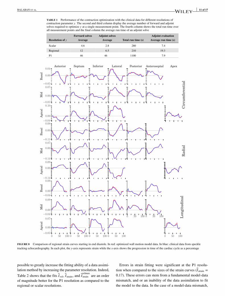
TABLE 1 Performance of the contraction optimization with the clinical data for different resolutions ofcontraction parameter 𝛾 . The second and third column display the average number of forward and adjointsolves required to optimize 𝛾 at a single measurement point. The fourth column shows the total run time overall measurement points and the final column the average run time of an adjoint solve

Forward solves Adjoint solves Adjoint evaluationResolution of 𝛾 Average Average Total run time (s) Average run time (s)

Scalar 4.6 2.8 280 7.4

Regional 12 6.5 210 19.3

P1 46 46 1100 7.9

FIGURE 8 Comparison of regional strain curves starting in end diastole. In red: optimized wall motion model data. In blue: clinical data from speckletracking echocardiography. In each plot, the y-axis represents strain while the x-axis shows the progression in time of the cardiac cycle as a percentage

possible to greatly increase the fitting ability of a data assimi-lation method by increasing the parameter resolution. Indeed,

Table 2 shows that the fits Ivol, Istrain, and Irelmaxstrain are an order

of magnitude better for the P1 resolution as compared to theregional or scalar resolutions.

Errors in strain fitting were significant at the P1 resolu-tion when compared to the sizes of the strain curves (Istrain =0.17). These errors can stem from a fundamental model-datamismatch, and or an inability of the data assimilation to fitthe model to the data. In the case of a model-data mismatch,

12 of 17 BALABAN ET AL.

TABLE 2 Relative misfit for different representation of 𝛾

Resolution of 𝛾 Ivol Istrain Irelmaxstrain

Scalar 0.044 1.5 0.27

Regional 0.024 1.1 0.16

P1 0.0037 0.17 0.029

the limitations of the model may play a role (see Section 4.1).Another cause of model-data mismatch is inaccuracy or noisein measurements, in which case, the model can be used toimprove the measurements. This is the case when models areused to regularize image-based motion.37,38

The SQP optimization algorithm that we used is a localsearch only, so that is possible that our fitting was suboptimal,possibly contributing to the mismatch in strain. Adding regu-larization has been shown to prevent such suboptimal resultsin fluid control problems [39 page 123]. This partially moti-vated our use of regularization in the contraction optimization(Equation 17).

The discrepancies between our model-based and measuredstrains are very small, however, when compared to the sizesof the largest strain curves of a given strain type, longitudinal,circumferential, or radial. This can clearly be seen in Figure 8

and in the low value of the metric Irelmaxstrain . This shows that our

method was able to accurately capture the larger amplitudefeatures of the heterogeneity in contraction. Such features areless prone to distortion by noise then those with smaller strainvalues and are therefore more relevant for potential medicaluse. However, the question of how much model resolutionis actually needed to provide medically useful informationremains an open one.

As a consequence of increased dimensionality in the opti-mization, estimating the contraction 𝛾 took just under 4times longer with the P1 resolution than the scalar resolu-tion. This was due to an increase in the number of forwardand adjoint evaluations needed at the higher resolution. How-ever, the average run time of an adjoint gradient evaluationdid not differ significantly in the P1 case. This near invari-ance of the gradient calculation cost to the number of opti-mization parameters is an advantage of the adjoint-gradientmethod. In the case of the regional resolution, the averageadjoint-gradient run time was nearly double that of the other2 cases. This was due to increased symbolic computationrequired by the software dolfin-adjoint to differentiate char-acteristic functions defined over each AHA segment. Thetotal run time for the scalar case was higher than for theregional case, despite the scalar case requiring fewer forwardand adjoint evaluations. This was due to a greater number ofNewton iterations required per forward solve in the scalarcase.

To test the effects of mesh resolution on the contractionestimation, we have considered alternative mesh resolutionsin Appendix C. The analysis shows that the tested increaseand decrease in the resolution of the mesh did not signif-icantly change the fit quality of the contraction estimation

(Table C1). There were, however, slight differences in thespatial average of the contraction field between the 3 casestested (Figure C1). This was most likely due to differences inthe quality of the discrete approximation of the work balanceequation (2).

In the current study, the resolution of the computationalmesh affected both the resolution of the contraction fieldand the resolution of the displacement-pressure variables inthe finite element model. The results of the mesh resolutiontests suggest our contraction field may have been too highlyresolved and that it might be beneficial to select the resolu-tion of the contraction variable independently of the mesh infuture studies. This would require specifying a set of basisfunctions for 𝛾 , which could be designed to allow for a goodfit of model to data while at the same time minimizing thenumber of degrees of freedom. Such a procedure has been pre-viously implemented for parameter estimation in groundwatermodelling.40

To test the accuracy of the contraction estimation, we haveconducted synthetic data tests for which the true contractionfield was known. The results of these tests show that ourdata assimilation is greatly effected by the sparsity of data.Indeed, the approximation of 𝛾 was an order of magnitude bet-ter with strains that had all 6 components and were definedeverywhere on the geometry, as compared to the regionallyaveraged strains limited to the tensor diagonal. This result didnot hold at the apex where the maximum errors were the samefor all 3 cases.

The regionally averaged strain representation is easier fora human to interpret and is widely used in medical research.However, for the purposes of building accurate personalizedmodels, more resolution of strain is highly advantageous. Thesynthetic tests also showed that our data assimilation is notgreatly effected by noise in the echocardiographic measure-ments. This is most likely due to our use of regularization,which favoured smoother solutions that averaged out theeffects of the noise.

In addition to noise in strain, we can also expect inaccura-cies in volume measurements from echocardiography. This isan issue for the estimation of the elastic parameter a, which weconducted purely from volume measurements. Experimentswith gel phantoms have quantified this inaccuracy for assess-ments of a single image.41 However, for the estimation ofthe elastic parameter a, relative differences in errors betweenimages are more relevant. These have to the best of our knowl-edge not been studied and so we have conducted estimationsof a with volume curves perturbed by a range of errors (seeAppendix 3.1). These experiments show that the estimatedstiffness parameter is indeed sensitive to volume errors. Theeffect on the average of the contraction field is, however,quite minimal. An alternative to the current stiffness estima-tion procedure would be to allow for greater spatial resolutionfrom strain measurements as per the contraction parameter.This might allow for a regularized stiffness field to averageout the effects of noisy measurements.

BALABAN ET AL. 13 of 17

The volume fit between model and data was close for the3 points in atrial systole, but differed in early isovolumiccontraction. Indeed, the model underestimated the measuredvolumes, indicating an overestimation of ventricular stiff-ness at these points. This is a consequence of fitting thestiffness parameters to the atrial systolic points, and not tothe points in early isovolumic contraction afterwards. If theeffects of contraction could be isolated from the effects ofelasticity, it would be possible to include these points in theelastic parameter fitting and possibly obtain a better match ofvolumes.

In our study, we personalized only a single elastic parametera, which was done for the sake of simplicity. Previous studieshave successfully estimated greater numbers of elastic param-eters for the reduced Holzapfel law9 and the fully orthortropicHolzapfel law.3 Such procedures could be potentially com-bined with our contraction estimation to increase the level ofmodel personalization. Another potential improvement of theelastic parameter estimation we used is the inclusion of aggre-gated geometry measures, such as short axis and long axisdiameters. Such measures have been shown to improve iden-tifiability of elastic parameters in experiments with mouseventricles.42

Several data assimilation studies5,6 have included objectivefunctionals consisting of strain and volume components withequal weighing given to both. We have shown that it maybe possible to improve such data assimilation procedures bytuning the relative weight of strain and volume components.Indeed, in the top right plot of Figure 3, there is a definite cor-ner in the strain-volume fitting space consisting of 4 pointsbeneath 𝛼 = 0.95. Choosing 𝛼 among these points gives a fairtrade-off between strain and volume matching whereas anychoice outside this corner simply worsens the fit of strain orvolume without much improving the other.

In Figure 3, we have shown how the parameters 𝛼 and 𝜆affect the fitting and smoothness metrics related to the con-traction field 𝛾 . Additionally, we have tested the effects ofvariations in 𝛼 and 𝜆 on the spatial average of the contrac-tion field. These experiments are presented in Appendix D.Figure D1 shows that varying 𝛼 in the region [0, 0.5] had lit-tle to no effect on the spatial average of 𝛾 , whereas increasesin 𝛼 outside of this region tended to increase the amount ofcontraction. This behaviour correlates with the value of Istrain

in (Figure 3 top right). Similarly, increasing 𝜆 beyond 0.001tended to increase the misfit in the data functional (Figure 3bottom right) and also increase the average amount of contrac-tion (Figure D1 right). We hypothesize that additional levelsof misfit in strain introduced by increasing 𝛼 beyond 0.5 andor 𝜆 beyond 0.001 lead to overestimating the amount of con-traction in our patient’s LV. However, we lack knowledge ofthe true amount of muscle contraction in the patient, whichcould be used to test the hypothesis. Further validation of themodel and data assimilation are needed.

4.1 Limitations

The results obtained in this article were limited by issuespertaining to the choice of mathematical model, quality ofclinical data, numerical stability, and the design of the dataassimilation algorithm. Firstly, the boundary conditions of theventricle wall motion model did not account for the effects ofthe right ventricular pressure on the septum and the mechan-ical coupling to the neighboring structures: left atrium, rightventricle, and pericardium.

The in vivo circumferential and radial motion at the basewas not incorporated into the model. Instead, some motionwas allowed by the basal spring, whose constant k needed tobe chosen. In the future, we would like to incorporate basalmotion data from the images into our personalized model.This would allow us to avoid having to make a choice of k andhopefully allow for the reproduction of in vivo basal motionin the personalized model.

During the atrial systole phase, we assumed 𝛾 = 0. Thisallowed for the estimation of passive properties separate fromcontraction. This assumption is appropriate for a healthyventricle but might be false in a diseased ventricle if musclerelaxation is sufficiently delayed.

Our mathematical model of wall motion neglected theeffects of viscoelasticity, tissue compressibility,43 inertia, andmyocardial sheet microstructure. Finally, the reference geom-etry that we used for our calculations came from an echocar-diographic image in which there was a nonzero level of bloodpressure. The blood pressures we used in our patient spe-cific model were off by the 2.8 kPa that we subtracted tohave 0 pressure in the reference geometry. This pressureadjustment meant that the elastic stiffness of the ventriclewas underestimated by our elastic parameter estimation, asthe mathematical model operated at a lower pressure thanmeasured in the patient’s heart.

The accuracy of the optimized motion model was limited byuncertainties in the clinical strain and volume measurements,which were related to echocardiographic image quality, imagesample rate, and speckle tracking algorithm accuracy. Pres-sure and volume measurements had to be synchronized, whichmight have lead to a potentially unphysiological loss of vol-ume in the iso-volumic relaxation phase of the in vivo PV loop(Figure 1).

Finally, there were several algorithmic limitations. Firstly,the optimized 𝛾 fields we computed may or may not have beenunique. For potential clinical applications, this is a concern asthe uniqueness of parameters relate to the reproducibility andconsistency of data obtained from a personalized model. Fur-thermore, our procedures for choosing the functional weights𝛼 and 𝜆 were not optimal. In both the synthetic and clinicaldata case, the weight values were chosen by parameter sweepsthat kept a single parameter fixed, which did not account forpossibly better 𝛼,𝜆 combinations lying outside of the areaswe tested. Finally, the SQP optimization algorithm that weused was a local search only, that is, only one minimum ofthe objective is calculated. Better parameter fits may be pos-

14 of 17 BALABAN ET AL.

sible with global optimization methods that explore multipleminima.

5 CONCLUSION AND FUTURE OUTLOOK

By using high-resolution data assimilation, we were able tocapture the detailed motion of a dyssynchronous LV in a com-putational model with an excellent fit of model observationsto data. This demonstrates the power of the data assimilationmethod, which can also be applied to other models and ormodel parameters.

In the future, the proposed method should be furtherimproved and tested on cohorts of patients. This wouldallow for the study of simulated contraction patterns amonggroups of patients that could lead to further understanding ofdyssynchrony.

6 AUTHOR DECLARATION

All of the clinical data for this study was collected with theapproval of the Norwegian national ethics committee, REC,and in accordance to the Helsinki Declaration of 1975, asrevised in 2000.

ACKNOWLEDGMENTS

Computations were performed on the Abel supercomputingcluster at the University of Oslo via Notur projects nn9316kand nn9249k.

Funding was provided by the Research Council of Nor-way via the Center for Biomedical Computing at SimulaResearch Laboratory (grant 179578), and via the Center forCardiological Innovation at Oslo University Hospital (grant203489).

REFERENCES

1. Sermesant M, Moireau P, Camara O, et al. Cardiac function estimation fromMRI using a heart model and data assimilation: Advances and difficulties.Med Image Anal. 2006;10(4):642–656.

2. Augenstein KF, Cowan BR, LeGrice IJ, Nielsen PM, Young AA. Method andapparatus for soft tissue material parameter estimation using tissue taggedmagnetic resonance imaging. J Biomech Eng. 2005;127(1):148–157.

3. Gao H, Li WG, Cai L, Berry C, Luo X. Parameter estimationin a Holzapfel–Ogden law for healthy myocardium. J Eng Math.2015;95(1):231–248.

4. Wang VY, Lam HI, Ennis DB, et al. Modelling passive diastolic mechanicswith quantitative MRI of cardiac structure and function. Med Image Anal.2009;13(5):773–84.

5. Mojsejenko D, McGarvey JR, Dorsey SM, et al. Estimating passive mechan-ical properties in a myocardial infarction using MRI and finite elementsimulations. Biomech Model Mechanobiol. 2014;14(3):633–647.

6. Sun K, Stander N, Jhun CS, et al. A computationally efficient formal opti-mization of regional myocardial contractility in a sheep with left ventricularaneurysm. J Biomech Eng. 2009;131(11):111001–111001-10.

7. Neumann D, Mansi T, Georgescu B, et al. Robust image-based estimationof cardiac tissue parameters and their uncertainty from noisy data, MedicalImage Computing and Computer-Assisted Intervention–MICCAI 2014. NewYork, NY: Springer; 2014:9–16.

8. Wong KC, Sermesant M, Rhode K, et al. Velocity-based cardiac contractil-ity personalization from images using derivative-free optimization. J MechBehav Biomed Mater. 2015;43:35–52.

9. Asner L, Hadjicharalambous M, Chabiniok R, et al. Estimation of passiveand active properties in the human heart using 3d tagged mri. Biomech ModelMechanobiol. 2015:1–19.

10. Hadjicharalambous M, Chabiniok R, Asner L, et al. Analysis ofpassive cardiac constitutive laws for parameter estimation using3D tagged MRI. Biomech Model in Mechanobiol. 2015;14(4):807–828.

11. Chabiniok R, Moireau P, Lesault P-F, et al. Estimation of tissue contractilityfrom cardiac cine-MRI using a biomechanical heart model. Biomechanicsand Model in Mechanobiol. 2012;11(5):609–630.

12. Xi J, Lamata P, Lee J, et al. Myocardial transversely isotropic mate-rial parameter estimation from in-silico measurements based on areduced-order unscented Kalman filter. J Mech Behav Biomed Mater.2011;4(7):1090–1102.

13. Marchesseau S, Delingette H, Sermesant M, et al. Preliminary specificitystudy of the Bestel-Clément-Sorine electromechanical model of the heartusing parameter calibration from medical images.J Mech Behav BiomedMater. 2013;20:259–71.

14. Delingette H, Billet F, Wong KCL, et al. Personalization of cardiac motionand contractility from images using variational data assimilation. IEEE TransBiomed Eng. 2012;59(1):20–24.

15. Sundar H, Davatzikos C, Biros G. Biomechanically-constrained 4Destimation of myocardial motion. Medical Image Computing andComputer-Assisted Intervention–MICCAI, London, UK, 2009. New York,NY: Springer; 2009:257–265.

16. Balaban G, Alnæs MS, Sundnes J, Rognes ME. Adjoint multi-start-basedestimation of cardiac hyperelastic material parameters using shear data.Biomech Model Mechanobiol. 2016;15(6):1–13.

17. Krishnamurthy A, Villongco CT, Chuang J, et al. Patient-specific models ofcardiac biomechanics. J Comput Phys. 2013;244:4–21.

18. Gjerald S, Hake J, Pezzuto S, Sundnes J, Wall ST. Patient–specific param-eter estimation for a transversely isotropic active strain model of left ven-tricular mechanics. Statistical Atlases and Computational Models of theHeart-Imaging and Modelling Challenges. New York, NY: Springer; 2015:93–104.

19. Holzapfel Ga, Ogden RW. Constitutive modelling of passive myocardium: astructurally based framework for material characterization. Philos Trans SerA Math Phys Eng Sci. 2009;367(1902):3445–75.

20. Land S, Niederer S, Lamata P, et al. Improving the stability ofcardiac mechanical simulations. IEEE Trans Biomed Eng. 2015;62(3):939–947.

21. Nardinocchi P, Teresi L. On the active response of soft living tissues. J Elast.2007;88(1):27–39.

22. Evangelista A, Nardinocchi P, Puddu PE, et al. Torsion of the human leftventricle: experimental analysis and computational modeling. Prog BiophysMol Biol. 2011;107(1):112–121.

23. Hospital OU. Acute feedback on left ventricular lead implantation loca-tion for cardiac resynchronization therapy (CCI impact). 2016. https://clinicaltrials.gov. Accessed September 1, 2016.

24. Cerqueira MD, Weissman NJ, Dilsizian V, et al. Standardized myocardialsegmentation and nomenclature for tomographic imaging of the heart a state-ment for healthcare professionals from the cardiac imaging committee ofthe Council on Clinical Cardiology of the American Heart Association.Circulation. 2002;105(4):539–542.

25. Bols J, Degroote J, Trachet B, et al. A computational method to assess the invivo stresses and unloaded configuration of patient-specific blood vessels. JComput Appl Math. 2013;246:10–17.

26. Gee MW, Förster C, Wall WA. A computational strategy for prestress-ing patient-specific biomechanical problems under finite deformation. Int JNumer Meth Biomed Eng. 2010;26(1):52–72.

27. Geuzaine C, Remacle JF. Gmsh: A 3-D finite element mesh generatorwith built-in pre-and post-processing facilities. Int J Numer Meth Eng.2009;79(11):1309–1331.

BALABAN ET AL. 15 of 17

28. Bayer JD, Blake RC, Plank G, Trayanova NA. A novel rule-based algorithmfor assigning myocardial fiber orientation to computational heart models.Annals of Biomed Eng. 2012;40(10):2243–2254.

29. Hood P, Taylor C. Navier-stokes equations using mixed interpolation. FiniteElem Meth Flow Prob. 1974:121–132.

30. Logg A, Mardal KA, Wells GN, et al. Automated Solution of DifferentialEquations by the Finite Element Method. New York, NY: Springer; 2011.

31. Balay S, Brown J, Buschelman K, et al. PETSc web page. 2015. http://www.mcs.anl.gov/petsc. Accessed September 1, 2016.

32. Li XS, Demmel JW. SuperLUDIST: A scalable distributed-memory sparsedirect solver for unsymmetric linear systems. ACM Trans Math Softw.2003;29(2):110–140.

33. Kraft D. A Software Package for Sequential Quadratic Programming. Ger-many: DFVLR Obersfaffeuhofen; 1988.

34. Farrell PE, Ham DA, Funke SW, Rognes ME. Automated derivation of theadjoint of high-level transient finite element programs. SIAM J Sci Comput.2013;35(4):C369–C393.

35. Pezzuto S, Ambrosi D, Quarteroni A. An orthotropic active–strain modelfor the myocardium mechanics and its numerical approximation. Eur JMech-A/Solids. 2014;48:83–96.

36. Finsberg H, Balaban G. High resolution data assimilation of car-diac mechanics. 2016. http://www.bitbucket.org/finsberg/cardiac_highres_dataassim. Accessed September 1, 2016.

37. Papademetris X, Sinusas AJ, Dione DP, Constable RT, Duncan JS.Estimation of 3-d left ventricular deformation from medical imagesusing biomechanical models. IEEE Trans Med Imaging. 2002;21(7):786–800.

38. Tuyisenge V, Sarry L, Corpetti T, et al. Estimation of myocardial strain andcontraction phase from cine mri using variational data assimilation. IEEETrans Med Imaging. 2016;35(2):442–455.

39. Gunzburger MD. Perspectives in Flow Control and Optimization.Philadelphia: Siam; 2002.

40. Tsai FTC, Sun NZ, Yeh WWG. Global-local optimization for parameterstructure identification in three-dimensional groundwater modeling. WaterResour Res. 2003;39(2):1043.

41. Aurich M, André F, Keller M, et al. Assessment of left ventricular vol-umes with echocardiography and cardiac magnetic resonance imaging:real-life evaluation of standard versus new semiautomatic methods. J Am SocEchocardiography. 2014;27(10):1017–1024.

42. Nordbø Ø, Lamata P, Land S, et al. A computational pipeline for quan-tification of mouse myocardial stiffness parameters. Comput Biol Med.2014;53:65–75.

43. Yin F, Chan C, Judd RM. Compressibility of perfused passive myocardium.Am J Physiol-Heart Circulatory Physiol. 1996;271(5):H1864–H1870.

How to cite this article: Balaban G, Finsberg H,Odland HH, Rognes ME, Ross S, Sundnes J, Wall S.High-resolution data assimilation of cardiac mechan-ics applied to a dyssynchronous ventricle. IntJ Numer Meth Biomed Engng. 2017;33:e2863.https://doi.org/10.1002/cnm.2863

APPENDIX A

SENSITIVITY OF ELASTIC PARAMETER TO ERROR IN ATRIALSYSTOLIC VOLUME MEASUREMENTS

To test the sensitivity of our estimated a parameter to uncer-tainty in volume measurements, we have conducted a seriesof estimations with various levels of volume perturbation.

TABLE A1 Sensitivity of the optimized material parameter a to errorsin volume measurements. The first column gives the perturbation of thevolume increase between measurement points 1-2 and 2-3, inpercent. The next 2 columns give the size of these perturbations inmilliliters with ΔV2 and ΔV3 referring to perturbations in the volumes ofthe second and third measurement points, respectively. In the fourth column,optimal a values are given. In all cases, the volume fit Ivol was lessthan 4 × 10 − 6

Perturbation ΔV2 ΔV3 a(%) (ml) (ml) (kPa)

−25 −1.2 −1.06 0.494

−15 −0.717 −0.636 0.469

−5 −0.239 −0.212 0.446

0 0 0 0.435

5 0.239 0.212 0.424

15 0.717 0.636 0.404

25 1.2 1.06 0.384

FIGURE A1 Sensitivity of the optimal average contraction 𝛾 to changes inthe parameter a. The upper and lower a values are based on estimating awith volume perturbations of ± 25% (Table A1). The middle value wasobtained by estimating a from in vivo volumes

We generated clean volume data using the computationalmodel using a = 0.435 kPa, the optimal value obtained fromthe clinical data. Perturbations in volume increases of sizes± 5,15,25% were added to this data, which were then usedas target for optimization. The resulting a values and per-turbations are shown in Table A1. The largest perturbationsresulted in the a values 0.494 kPa and 0.384 kPa, representingcirca ± %13 change from the original a value.

The resulting average value of 𝛾 is shown in Figure A1for the extreme cases with 𝛼 = 0.494 and 𝛼 = 0.384 . Forreference, we also include the average value of 𝛾 using𝛼 = 0.435.

APPENDIX B

SENSITIVITY OF ESTIMATED PARAMETERS TO SPRINGCONSTANT

The spring boundary condition that we used at the ven-tricular base has a significant effect on the simulated cav-ity volumes calculated by the model. This is due to the

16 of 17 BALABAN ET AL.

TABLE B1 Sensitivity of optimal a value to choice of spring constant k

k 10 − 8 10 − 7 10 − 6 10 − 5 10 − 4 10 − 3 0.01 0.1 1 10 100 ∞

a 0.875 0.875 0.875 0.875 0.873 0.873 0.849 0.684 0.435 0.375 0.366 0.365

FIGURE B1 Sensitivity of the spatially averaged contraction 𝛾 to thechoice of spring constant k

cross-sectional area of the cavity being large at the ventric-ular base. Therefore, we can expect the choice of k to havean effect on the optimal parameters calculated by our dataassimilation.

To quantify this effect, we have conducted a sensitivityanalysis, starting with the effect of k on the optimized elas-tic parameter a. We repeated the elastic parameter fittingdecribed in Section 3.1 and varied the k-value from 0.001 to100.0. We also considered the case k = ∞, denoting a com-pletely rigid boundary held by Dirichlet boundary conditions.The effect of the choice of k on the optimal value of a is shownin Table B1. The table shows that the optimal a varies from0.365 kPa to 0.875 kPa depending upon how the k parameteris set.

We also tested the sensitivity of the contraction 𝛾 at P1 res-olution to k by repeating the estimation of 𝛾 with the variousk and a pairs obtained in the previous experiment. For each k,a pair, we have plotted the spatial average of contraction 𝛾 ateach measurement point in Figure B1. The results show up toa 20% variation in 𝛾 and very little variation for the choices ofk greater than or equal to 1.0. For some of the values of k< 1.0,our homotopy Newton solver was unable to secure conver-gence during the optimization. Curves corresponding to thesecases are drawn only to the point before the nonconvergenceoccurred.

APPENDIX C

EFFECT OF MESH RESOLUTION ON ESTIMATEDCONTRACTION AT P1 RESOLUTION

Ventricular meshes were generated by Gmsh27 with 3different resolutions controlled by the parameter“Mesh.CharacteristicLengthFactor.” This parameter wasgiven the values 1.0, 0.65, and 0.45, which resulted inmeshes with 549, 1262, and 2261 vertices, respectively.Using the 3 meshes, we estimated contraction fieldsfrom the in vivo data. The average value of 𝛾 is shownfor these 3 cases in Figure C1. Fit quality is comparedin Table C1.

FIGURE C1 Spatial average of contraction 𝛾 for 3 different meshresolutions

TABLE C1 Relative misfit for different mesh resolutions

Number of elements Ivol Istrain Irelmaxstrain

549 0.0033 0.17 0.029

1262 0.0037 0.17 0.029

2661 0.0043 0.18 0.031

APPENDIX D

SENSITIVITY OF CONTRACTION SIZE TO CHOICES OFAND 𝜆

On the basis of the trade-off curves in Figure 3, we chose theoptimization weights 𝛼 = 0.95 and 𝜆 = 0.01 for the person-alization of our wall motion model to the in vivo data. Toshow the effect of these choices on the optimized contractionfield 𝛾 , we have varied the 𝛼 and 𝜆 values and plotted the spa-tial averages of the resulting contraction fields. The resultsshow that the amount of contraction tends to increase propor-tionally to both 𝛼 and 𝜆 beyond the thresholds 𝛼 = 0.5 and𝜆 = 0.001.

APPENDIX E

ESTIMATION OF NOISE IN ECHO SPECKLE TRACKING STRAINMEASUREMENTS

To increase the relevance of the synthetic tests, we consid-ered a set of regional strains that contained noise. This noisewas modelled as an additive Gaussian process to imitate the

TABLE E1 Mean and covariance of a Gaussian noise summand estimatedfrom patient drift values in circumferential (C), radial (R), and longitudinal(L) directions

Covariance × 10 − 4

C R L Mean

C 1.43 0.73 0.66 0.006

R - 6.8 6.31 −0.013

L - - 7.26 0.01

BALABAN ET AL. 17 of 17

FIGURE D1 Sensitivity of the spatially averaged contraction 𝛾 to variations in optimization weights 𝛼 and 𝜆. Left: 𝜆 = 0 and 𝛼 is varied. Right: 𝛼 = 0.95 and𝜆 is varied

accumulation of tracking errors in EchoPac’s image-basedstrain calculations. The mean and variance of a summandin the Gaussian process were estimated from our in vivostrain data of a single patient. From these data, the sam-ple means and variances of the drift values were dividedby the number of measurement points to approximate the

noise in a single measurement. The mean and covariance ofthis single measurement point noise are given in Table E1.Theoretically, error-free strain curves would have no driftgiven stable conditions in the heart. This motivates the useof the drift values in order to approximate the trackingerror.