
High Pressure Study of Gd5(SixGe1 x 4 Giant...
131
NORTHWESTERN UNIVERSITY High Pressure Study of Gd 5 (Si x Ge 1-x ) 4 Giant Magnetocaloric Materials Using X-ray Magnetic Circular Dichroism A DISSERTATION SUBMITTED TO THE GRADUATE SCHOOL IN PARTIAL FULFILLMENT OF THE REQUIREMENTS for the degree DOCTOR OF PHILOSOPHY Field of Materials Science and Engineering By Yuan-Chieh Tseng EVANSTON, ILLINOIS June 2009
Transcript of High Pressure Study of Gd5(SixGe1 x 4 Giant...

NORTHWESTERN UNIVERSITY
High Pressure Study of Gd5(SixGe1−x)4 Giant Magnetocaloric Materials Using
X-ray Magnetic Circular Dichroism
A DISSERTATION
SUBMITTED TO THE GRADUATE SCHOOL
IN PARTIAL FULFILLMENT OF THE REQUIREMENTS
for the degree
DOCTOR OF PHILOSOPHY
Field of Materials Science and Engineering
By
Yuan-Chieh Tseng
EVANSTON, ILLINOIS
June 2009

2
c© Copyright by Yuan-Chieh Tseng 2009
All Rights Reserved

3
ABSTRACT
High Pressure Study of Gd5(SixGe1−x)4 Giant Magnetocaloric Materials Using X-ray Magnetic
Circular Dichroism
Yuan-Chieh Tseng
The role of Si-doping in enhancing the magnetic ordering temperature (Tc) of Gd5(SixGe1−x)4
giant magnetocaloric compounds was investigated using x-ray magnetic circular dichroism (XMCD)
and diamond anvil cell (DAC) techniques. The purpose of the study is to understand the mecha-
nism of doping-induced ferromagnetic order in these compounds that may advance the magnetic
refrigeration technology. The results demonstrate that hydrostatic pressure leads to similar effects
as Si-doping for x≥ 0.125 because the P -T phase diagram reproduces the most notable features of
the x-T phase diagram, indicating that the magnetic properties of these compounds are volume-
driven. The low-x (0 < x ≤ 0.75) region exhibits an inhomogeneous magneto-structural ground
state featured by a mixed antiferromagnetic (orthorhombic (II))−ferromagnetic (orthorhombic
(I)) phase at low temperature. Pressure was found to remove this magneto-structural inhomo-
geneity by fully restoring the magnetization that is obtained for x ≥ 0.125. However, unlike the
nearly constant dTc/dP obtained for 0.125 ≤ x < 0.5, dTc/dP of the low-x samples is strongly
4
x-dependent. This suggests that the emergence of the ferromagnetic order from within the anti-
ferromagnetic phase of Gd5Ge4 parent compound cannot be simply described as a volume-effect
due to the existence of the magneto-structural inhomogeneity. Finally, the quantitative corre-
spondence between Si-doping and hydrostatic pressure was examined in order to know if the
properties of these materials are monotonically volume-dependent. It was found that Si-doping
increases Tc much more effectively than pressure, by a factor of ∼ 11 for a given volume reduc-
tion. A local lattice contraction was found around Si atoms as a result of the substitution of
Ge by the smaller Si atoms resulting in a remarkably high local chemical pressure. This local
contraction results in a stronger Si 3p-Gd 5d orbital hybridization benefiting the indirect fer-
romagnetic exchange and hence responsible for a more effective Tc increase, overthrowing the
concept prior to this study that macroscopic volume contraction is the major course determining
Tc increase.
Approved
Professor Michael J. BedzykDepartment of Materials Science and EngineeringNorthwestern University Evanston, IL
Final Examination Committee:Prof. Michael J. Bedzyk, ChairDr. Daniel HaskelDr. George SrajerProf. Christopher M. WolvertonProf. Mark C. Hersam

5
Acknowledgements
It is a great pleasure to thank the many people who made this thesis possible. My utmost
gratitude goes to my Argonne advisor Dr. Daniel Haskel because of his selfless guidance through-
out my graduate studies. I greatly appreciate his mentoring based on trust and friendship −
working with him is an unforgettable experience. I also thank Prof. Bedzyk and Dr. Srajer for
providing me with the opportunity to work at Argonne National Laboratory. I also appreciate
Prof. Wolverton and Prof. Hersam for their valuable comments in my final exam. In addition,
I need to thank Dr. N. M Souza-Neto for the precious partnership in all experiments, and also
Dr. S. Sinogeikin and Dr. Y. Ding for enriching my knowledge in high pressure field. Besides,
Dr. Y. Choi, Dr. M. A. Laguna-Marco, Dr. J. C. Lang who provided important suggestions to
my thesis deserve my acknowledgement as well. I am very thankful for having been a member
of the Magnetic Materials Group and I appreciate every single person in this group who ever
helped me over the past 3 years.
I can’t neglect Prof. V. K. Pecharsky, Prof. K. A. Gschneidner, Dr. Ya. Mudryk, and
Dr. D. Paudyal at Ames Laboratory for their remarkable contributions to the magnetocaloric
materials project. I also thank my Northwestern colleagues, V. Kohli, Z. Feng, M. McBriarty,
J. Alaboson, J. Emery, S. Christensen, J. Klug, and C.Y. Leung for enriching my graduate life.
I would also like to express my gratitude to Ching-Hui for joining my life in my last year at
Northwestern, making my life never alone. Moreover, I especially thank my best roommate and
colleague, Jui-Ching (Phillip) Lin for accompanying me to Northwestern a few years ago and

6
walking through different life experience together. I appreciate the encouragements given by
a few close friends including Wei-Chih, Nicole, Shu-Te, Shan-Wei, Meng-Chun, Ching-Hsuan,
Yu-Chen, Yi-Kai, Shih-Han, and church members like Emily, Hsieh-Ke, Past. Wu, Dr. Lin and
Prof. Chen. My younger brother, Hsin-Wu, has also been my loyal supporter and I wish him the
best for his study at the Univ. of Florida. Finally, I would like to dedicate this dissertation to
my dear parents and family in Kaohsiung, Taiwan−it is their encouragements that gave me the
initial motivation to study in the U.S. and their long-lasting supports that helped me persevere
in despite of all the difficulties.
Yuan-Chieh Tseng
Northwestern University, June 2009

7
Table of Contents
ABSTRACT 3
Acknowledgements 5
List of Tables 10
List of Figures 11
Chapter 1. Introduction 15
1.1. Giant magnetocaloric effect and Gd5(SixGe1−x)4 compounds 15
1.2. The role of Si-doping in Gd5(SixGe1−x)4 24
1.3. Volume effect in Gd5(SixGe1−x)4 24
1.4. Motivation for high pressure study 25
Chapter 2. Introduction to synchrotron techniques 28
2.1. X-ray magnetic circular dichroism (XMCD) 28
2.2. X-ray absorption fine structure (XAFS) 38
2.3. X-ray powder diffraction (XRD) 42
Chapter 3. High pressure experimental setup 46
3.1. High-pressure XMCD beamline setup 46
3.2. Diamond anvil cell (DAC) 48
3.3. Sample preparation 50

8
3.4. Pressure calibration 50
Chapter 4. Role of Si-doping in enhancing ferromagnetic interactions in Gd5(SixGe1−x)4
compounds 57
4.1. Introduction 57
4.2. Experiment 58
4.3. Results for Gd5(Si0.125Ge0.875)4 and Gd5(Si0.5Ge0.5)4 compounds 59
4.4. Discussions for Gd5(Si0.125Ge0.875)4 and Gd5(Si0.5Ge0.5)4 63
4.5. Results and discussions for Gd5(Si0.375Ge0.625)4 67
4.6. Conclusion 69
Chapter 5. Emergence of ferromagnetic order from within antiferromagnetic phase of
Gd5Ge4: pressure studies of low-x region 70
5.1. Introduction 70
5.2. Experiment 71
5.3. Results 73
5.4. Discussion 79
5.5. Modified phase diagram of Gd5(SixGe1−x)4 86
5.6. Conclusion 90
Chapter 6. Quantitative discrepancy between Si-doping and pressure effects upon
Gd5(SixGe1−x)4 compounds 91
6.1. Introduction 91
6.2. Experiment 92
6.3. Results 94

9
6.4. Discussion 100
6.5. Conclusion 106
Chapter 7. Summary and future work 108
7.1. Thesis summary 108
7.2. Future work 110
References 114
Appendix A. Local structure analysis using IFEFFIT calculation 121
A.1. Introduction to IFEFFIT 121
A.2. Data analysis process 121
Appendix B. FDMNES calculations 127
B.1. Introduction 127
B.2. Program inputs 127
B.3. Examples 130

10
List of Tables
1.1 MCE of different materials 20
6.1 Si and Ge interatomic distance change determined by K -edge XAFS 103

11
List of Figures
1.1 Schematic illustration of magnetic refrigeration cycle 17
1.2 The entropy-temperature diagram of the MCE materials 18
1.3 Analogy between magnetic refrigeration and traditional vapor-compressed
refrigeration 19
1.4 Crystal structures of Gd5(SixGe1−x)4 22
1.5 Phase diagram of Gd5(SixGe1−x)4 23
2.1 Schematic illustration of the circularly polarized x-ray induced electronic
transition responsible for XMCD 29
2.2 helicity-dependent XAS and XMCD spectra 30
2.3 Temperature dependence of the coercive field (Hc) for ε-Fe2O3 nanoparticles 33
2.4 Temperature-dependence of morb, mspin and morb/mspin for ε-Fe2O3
nanoparticles 34
2.5 Schematic illustration of the vectorial-probe characteristic of XMCD 35
2.6 Magnetic-field dependence of out-of-plane XMCD signal for Mn and Ru in
SrRuO3/SrMnO3 multilayer 36
2.7 Schematic illustration of the spin configuration of SrRuO3/SrMnO3 multilayer 37
2.8 Schematic illustration of a XAFS process 39

12
2.9 XAFS analysis process 41
2.10 Schematic illustration of the Bragg diffraction 42
2.11 Angle-dispersive powder diffraction setup 44
2.12 2-D diffraction image pattern and 2θ diffraction pattern of Gd5(SixGe1−x)4 45
3.1 Schematic illustration of the experimental high-pressure XMCD setup 47
3.2 Configuration of the diamond anvil cell, cold finger extension, and
electromagnet 49
3.3 Cu XAFS pressure calibration 53
3.4 Pressure-dependent ruby R-line fluorescence spectra 55
3.5 Portable ruby fluorescence detector 56
4.1 Gd L3 -edge XMCD signal as a function of temperature for P = 0.25 and
14.55 GPa for Gd5(Si0.125Ge0.875)4 60
4.2 XMCD as a function of temperature for different applied pressures for
Gd5(Si0.125Ge0.875)4 and Gd5(Si0.5Ge0.5)4 61
4.3 Magnetic phase diagram as a function of Si concentration and applied
pressure 62
4.4 dTc/dP comparison for Gd5(Si0.125Ge0.875)4, Gd5(Si0.375Ge0.625)4, and
Gd5(Si0.5Ge0.5)4; the P -T phase diagram of Gd5(Si0.375Ge0.625)4 68
5.1 Lattice parameters and unit-cell volume of x-dependent Gd5(SixGe1−x)4 72
5.2 Temperature-dependent dc magnetization of Gd5(SixGe1−x)4 73

13
5.3 X-ray diffraction pattern of Gd5(SixGe1−x)4 at T = 17 K and Rietveld
refinements 75
5.4 Gd L3 -edge XMCD signal taken at P = 9.2 GPa for Gd5(Si0.025Ge0.975)4 76
5.5 Temperature-dependent Gd L3 -edge XMCD for Gd5(Si0.025Ge0.975)4,
Gd5(Si0.05Ge0.95)4, and Gd5(Si0.075Ge0.925)4 at ambient condition 77
5.6 Temperature-dependent Gd L3 -edge XMCD for Gd5(Si0.025Ge0.975)4,
Gd5(Si0.05Ge0.95)4, and Gd5(Si0.075Ge0.925)4 at various pressures 78
5.7 (a)Temperature-dependent saturation magnetization and (b) dTc/dP for
Gd5(Si0.025Ge0.975)4, Gd5(Si0.05Ge0.95)4, and Gd5(Si0.075Ge0.925)4 79
5.8 Modified magnetic phase diagram of Gd5(SixGe1−x)4 88
5.9 Modified structural phase diagram of Gd5(SixGe1−x)4 89
6.1 Comparison of XRD at selected pressure points for Gd5(Si0.125Ge0.875)4 95
6.2 XRD and Rietveld refinement for Gd5(Si0.125Ge0.875)4 at P = 7 GPa 96
6.3 Pressure-dependence of three lattice constants from ambient to 8 GPa for
Gd5(Si0.125Ge0.875)4 97
6.4 Lattice constant change and related volume change with pressure and
Si-doping, and their corresponding Tcs for Gd5(Si0.125Ge0.875)4 99
6.5 Magnitude of Fourier transform (FT) of Ge and Si K -edge XAFS spectra 102
6.6 Si and Ge K -edge experimental and simulated XANES and XMCD for
Gd5(Si0.125Ge0.875)4 104
6.7 Schematic illustration of the local contraction effect present in crystal lattice105

14
6.8 Schematic illustration of FM percolation in Gd5(SixGe1−x)4 106
A.1 Ge K -edge XAFS raw data with background removal and k -dependent
spectrum 122
A.2 ARTEMIS interface with FEFF paths 123
A.3 FEFF fitting parameters 124
A.4 FEFF fitting results 125
A.5 k-dependent and the Fourier transform of Ge K -edge XAFS with FEFF
fitting results 126
B.1 Basic codes for FDMNES calculation 128
B.2 Flow-chart for a complete FDMNES calculation process 129
B.3 Si K -edge XMCD and XANES spectra collected from FDMNES calculation130
B.4 Ge K -edge XMCD and XANES using different convolution width in
FDMNES calculation 131

15
CHAPTER 1
Introduction
1.1. Giant magnetocaloric effect and Gd5(SixGe1−x)4 compounds
Attention to environmental and energy issues has been on the rise in recent years, with
people becoming aware that the earth’s environment is gradually destroyed and the limited
energy resources are being over consumed by human activities. Global warming is considered
one of the most severe, requiring prompt strategies. Our current vapor-compressed refrigerant
technology is inefficient in electricity consumption, and its usage of chlorine-based refrigerant
results in fairly high greenhouse gas emission and ozone layer depletion which are responsible for
the global warming effect. To circumvent this, an alternative concept using solid state materials
as refrigerant was created. The key principle behind this concept is the magnetocaloric effect
(MCE)[1], where it harnesses the degree of ordering of nuclear or electronic magnetic dipoles
in order to reduce a material’s temperature and allow the material to serve as a refrigerant
(Fig. 1.1)[2]. This phenomenon was originally discovered in iron by Warburg[1] and explained
independently by Debye [3]and Giauque [4]. The cooling capability of the MCE is reflected
by the magnetic entropy (∆SM) and the adiabatic temperature (∆Tad) change upon applied
magnetic field, and these two parameters can be expressed as:

16
(1.1) ∆SM(T,4H) =
∫ H2
H1
(∂M(T,H)
∂T)HdH
(1.2) ∆Tad(T,4H) = −∫ H2
H1
(T
C(T,H))H
(∂M(T,H)
∂T)HdH
M, C and H represent the magnetization, the heat capacity of the material and the applied
magnetic field, respectively. The thermodynamics of the MCE in terms of ∆SM and ∆Tad is
illustrated in Fig. 1.2 [5].The analogy between a vapor-compressed and a magnetic refrigerant
is illustrated in Fig. 1.3 [6]. Conceptually, without emitting greenhouse gas and free of ozone-
depleting refrigerant, the magnetic refrigeration can perform as a more environmentally-friendly
counterpart. The MCE concept has been practical at very low temperature [5], but in order to
improve magnetic refrigeration technology to the household near room temperature refrigeration
based on the MCE is imperatively necessary.

17
+ H
Q
H = 0
+ Q
T
T + Tad
T
T Tad
T
Adiabatic process
Adiabatic process
Figure 1.1. Schematic illustration of magnetic refrigeration cycle. The MCE ma-terial is placed in an isolated environment (adiabatic condition). When a magneticfield (H) is applied, the magnetic dipoles are aligned. Since the process is adia-batic, the magnetic entropy is not reduced yet, thereby increasing the temperatureof the MCE material (T+∆T). The added heat can be removed by coolant suchas fluid or gas (-Q), while H is still held to prevent magnetic dipoles from re-absorbing the heat. Once the heat is removed, the MCE material undergoes anadiabatic process again to retain total entropy but H is decreased. The thermalenergy will cause magnetic dipoles to overcome H, hence reducing the temperatureof the material (T-∆T). At this moment, the MCE material will be contacted withthe substance wanted to be refrigerated. Because the MCE material is cooler thanthe substance, the heat will be transferred to the MCE material (+Q) finally toachieve the cooling purpose. Figure is reproduced from Ref. [2]

18
Figure 1.2. The entropy-temperature diagram taken from Ref. [5] illustrates themagnetocaloric effect. S0, T0 represent the entropy and temperature status withoutapplied field, and S1 and T1 represent those with applied filed. The solid linesrepresent the total entropy change with (S(H1)) and without (S(H0)) applied field.The dotted line represent the electronic and lattice (non-magnetic) entropy change,and the dashed lines represent the magnetic entropy change with (SM(H1)) andwithout (SM(H0)) applied field. The horizontal arrow and vertical arrow representthe change of ∆Tad and ∆SM with applied field, respectively.

19
T T+ ΔTHeat
rejection
T- ΔT Cool system
Heat
rejection
P = 0 P > 0 P = 0
H = 0 H > 0 H = 0
T T+ ΔT T- ΔT
Cool system
Figure 1.3. Analogy between magnetic refrigeration and traditional vapor-compressed refrigeration. In principle, the thermodynamic cycle used in magneticrefrigeration can replace the Carnot cycle used in traditional refrigeration for itperforms better efficiency (∼ 30 to 60 % of the Carnot cycle depending on appliedfield [1]) and is free to ozone-depleting coolants. Figure is reproduced from Ref.[6].

20
Material Tc(K) ∆H(T) ∆S(J/kgK) ∆Tad(K) Reference
La(FexSi1−x)H 274−291 2−5 -24−-28 7−13 [7-9]Mn(AsxSb1−x) 230−318 2−5 -18−-32 4.7−13 [10,11]
La(Ca,Sr)MnO3 230−263 1.5−5 -3.8−8 < 3 [12,13]Gd5(SixGe1−x)4 80−275 2−5 -14−-19 12−16 [14,15]Tb5(SixGe1−x)4 50−110 5 -20 - [16]Dy5(SixGe1−x)4 ∼ 65 5 -34 - [17]
Table 1.1. Entropy change, ∆SM and adiabatic temperature change, ∆Tad, occur-ring at the transition temperature Tc at different applied filed increase, ∆H, formaterials displaying the giant MCE.
There has been several compounds displaying near or above room temperature MCE reported
in recent studies. These include the series of La(Fe, Si)H [7, 8, 9], Mn(As, Sb) [10, 11],
La(Ca, Sr)MnO3 [12, 13], and R5(Si,Ge)4 [14-17]. Their MCE parameters (∆SM, ∆Tad) and
Curie temperatures (Tc) are present in Table 1. Among all candidate magnetocaloric materials,
R5(SixGe1−x)4 where R is a rare earth (Gd, Tb, Dy) has drawn much attention due to its very
strong coupling between structural and magnetic properties, leading to a giant MCE and making
itself a competitive candidate. The intriguing crystal structures, composed of Gd containing
slabs, together with the magnetic coupling mechanisms within and between the slabs, have been
the subject of intense research. The phase transitions obtained in these materials usually involve
change of crystal structure, such as breaking or forming of inter-slab Si(Ge) covalent bonds (Fig.
1.4) [6]. If the structural change occurs concomitantly with a magnetic transition, it results in a
1st order magneto-structural transition. In such case, the change in structural entropy is added to
the magnetic entropy change and the MCE of the material is greatly enhanced. Gd5(SixGe1−x)4
is renowned for its sizable MCE which could result in adiabatic temperature changes as high as
16 K [13, 18, 19]. More importantly, its 1st order magneto-structural transition responsible for

21
the giant MCE can be tuned to reach ∼ 275 K, displaying great potential for room temperature
(R.T.) operation of a magnetic refrigerant [18-23].
The building blocks of the crystal structure of Gd5(SixGe1−x)4 are the atomic-slabs shown
in Fig. 1.4. The slabs contain three inequivalent crystallographic sites for Gd ions and two for
Si(Ge) (T2 and T3, 25 % occupancy for each). The third crystallographic site for Si(Ge) is located
between slabs (T1, 50 % occupancy). This particular site is key because it effectively controls
the degree of atomic-interactions between slabs, as well as playing a key role in modifying the
crystal structures and magnetic properties [14, 19]. Figure 1.5 [6] shows the magnetism- and
structure- related phase diagram of Gd5(SixGe1−x)4. There are three extended substitutional
solid solutions in the phase diagram. First is with Gd5Si4 type structure (0.5 < x ≤ 1.0)
where the material’s paramagnetic phase (PM) exhibits fully connected Si(Ge) covalent bonds,
orthorhombic I (O(I)) structure. Second is with Gd5Si2Ge2 type structure (0.24 ≤ x ≤ 0.5) where
only half of Si(Ge) covalent bonds are present at monoclinic (M), PM phase. The third is with
Gd5Ge4 type structure (0 ≤ x ≤ 0.2), and the material’s PM phase displays an orthorhombic
II (O(II)) structure with broken Si(Ge) covalent bonds. Interestingly, the material displays x-
independent (0 < x ≤ 1.0), Si(Ge) bond-connected O(I) structure for ferromagnetic (FM) state.
In addition, an O(II), antiferromagnetic (AFM) intermediate phase is only present for 0 ≤ x ≤
0.2.

22
O(I) M O(II)
T2
T3
T1
Gd
Si/Ge
Figure 1.4. Crystal structures for Gd5(SixGe1−x)4 compounds. All Gd ions arelocated inside the slabs, while Si(Ge) can occupy either inter-slab (T1) or intra-slab (T2, T3) crystallographic sites. O(I), M and O(II) represent orthorhombic(I), monoclinic and orthorhombic (II), respectively. The presence or absence ofcovalent Si(Ge) bonds between the slabs is what distinguishes between the variousstructures. Figure is reproduced from Ref. [6].

23
x(Si)
0.0 0.2 0.4 0.6 0.8 1.0
Tem
pera
ture
(K
)
0
50
100
150
200
250
300
350
Ferromagnetic
Paramagnetic
AFM
O(I)
O(II)
M
M
O(II)
O(I)
Figure 1.5. Phase diagram of Gd5(SixGe1−x)4. Different crystal structures arethereby illustrated for different magnetic phases − O(II) for AFM and P in low xregion (0 ≤ x ≤ 0.2), M for PM in the middle of region (0.24 ≤ x ≤ 0.5), and O(I)for all FM (0 < x ≤ 1.0) but for PM only in high x region (0.5 < x ≤ 1.0). Figureis reproduced from Ref. [6].

24
1.2. The role of Si-doping in Gd5(SixGe1−x)4
A valuable feature of Gd5(SixGe1−x)4 is that Tc can be linearly increased by Si-doping, as
shown in Fig. 1.5. In particular, the ordering temperature is tunable from ∼ 30 to ∼ 275 K (0
< x ≤ 0.5) by adjusting the Si/Ge ratio without losing the giant MCE [25]. This expands the
operational temperature range of magnetic refrigeration based on this compound. However, this
striking feature disappears when the Si-content is larger than x = 0.5, where a purely, 2nd order
FM(O(I))→ PM(O(I)) transition takes place on warming (0.5 < x ≤ 1.0) without a concomitant
structural change, as also shown in Fig. 1.5 [18, 20]. This limits the usage of this material as
a magnetic refrigerant for applications below 275 K. Thus, in order to extend the giant MCE
towards R.T. in these and related materials, understanding the role of Si-doping has become an
important goal. Most of the relevant studies focused on certain interesting compositions (x = 0,
0.125, 0.5), sporadically exploring the fundamental knowledge of their magnetic and structural
properties and MCEs [19, 20, 26, 27]. Nevertheless, a systematic effort aimed at unveiling the
mechanism by which Si enhances Tc is missing. This effort is essential as it will shed light into
possible routes to achieve higher ordering temperature for the giant MCE materials, critically
needed for true R.T. magnetic refrigeration based on these and related compounds.
1.3. Volume effect in Gd5(SixGe1−x)4
Having smaller atomic size than Ge, Si’s role in occupying three inequivalent crystallographic
sites (Fig. 1.4) is to exert chemical pressure upon the lattice causing a reduction in unit cell vol-
ume. This volume reduction directly enhances both intra- and inter-slab magnetic interactions,
resulting in an increase of the FM ordering temperature. In particular, the volume reduction

25
also leads to the reforming of inter-slab bonds, converting either O(II) or M into O(I) structure
which favors the FM phase [6, 10, 16].
The macroscopic volume-effect obtained with atomic substitution suggests that it itself ought
to be the dominant course in modifying the material’s properties. Until now, a few pressure
studies were carried out to verify this hypothesis. Morellon et al. [28] reported that these
compounds exhibit a pressure-induced increase of the ordering temperature dTc/dP = 0.3 and
3.0 K kbar−1 for x = 0.8 and 0 ≤ x ≤ 0.5, respectively. Another work by the same authors
shows that pressure can convert Gd5Ge4 AFM-O(II) into FM-O(I) phase with dTc/dP = 4.8
K kbar−1 by reforming the inter-slab bonds [29]. Mudryk et al. [26] found that a M → O(I)
structural transition can be induced by applying pressures of ∼ 2.2 GPa in an x = 0.5 sample.
These preliminary findings indicate that pressure does stabilize the FM phase by converting the
structure from larger volume (O(II) or M) into smaller one (O(I)), similar to the effect of Si-
doping. Despite these findings, whether the magnetic/structural transitions are driven solely by
macroscopic volume effects is unclear, i.e. whether Si-doping in Gd5(SixGe1−x)4 simply reduces
the macroscopic volume and hence an equivalent effect is obtained with applied pressure.
1.4. Motivation for high pressure study
One common aspect of all previous pressure studies is their limitation to the low pressure
range. Extending this work to higher pressures is critical to unveil the correspondence between
Si-doping and pressure. Most pressure- and magnetism- related research in Gd5(SixGe1−x)4 was
done using the strain-gauge technique in a piston-cylinder, which can only provide pressures up
to 1 GPa (10 kbar) [28, 29]. To date, the highest pressure applied to Gd5(SixGe1−x)4 was 2.5
GPa [26]. This limitation restricts the correspondence study to a very narrow range and thus

26
leaves key questions unsolved. Besides, the low-x region (0 ≤ x ≤ 0.2; Fig. 1.5) displays an AFM
intermediate phase with low saturation magnetization, which is not present at higher Si content.
The mechanism that leads to the emergence of the FM order from Gd5Ge4 with pure AFM ground
state is unclear. In particular, the truth that whether the low-x region should be described
as a frustrated magnet with competing FM and AFM interactions, or a magneto-structural
mixed phase AFM(O(II))-FM(O(I)), hasn’t been examined. A pressure study combined with
x-ray powder diffraction at ambient condition could solve these questions which are not fully
addressed in Ref. [29] also due to pressure limitation. The magnetic properties measurements
of previous pressure-studies were primarily carried out in superconducting quantum interference
device (SQUID). The SQUID has very limited space for sample loading, and can’t avoid detecting
the paramagnetic or diamagnetic backgrounds usually displayed by most of the matters. These
factors limit the usage of certain pressure cells that can yield higher pressures.
In order to unambiguously determine the correlation between Si-doping and pressure, high-
pressure (HP) studies (up to ∼ 20 GPa) were conducted on Gd5(SixGe1−x)4 in this work. The
work was carried out by combining synchrotron techniques with a setup especially dedicated
to HP studies, where a diamond anvil cell (DAC) was incorporated. This combined technique
provides a better way to isolate the effects of volume reduction upon the magnetic/structural
transitions by ruling out doping-induced effects, such as (a) nonrandom distribution of Si(Ge)
among the three inequivalent sites [30], (b) volume-independent modifications to the electronic
structure due to differences in Ge 4p and Si 3p wave functions, and (c) phase separation or
spatially-inhomogeneous distribution of Si dopants depending on the conditions of the material’s
synthesis [31]. Within this approach, the correspondence between Si-doping and pressure was
investigated both qualitatively and quantitatively. Especially, we carried out the HP magnetic

27
properties measurements using x-ray magnetic circular dichroism (XMCD) which is renowned
for probing element-specific magnetism (described in Chapter 2). This work basically covers
pressure studies for most of the interesting regions of the phase diagram, including Ge-rich (0 <
x < 0.1) and middle (0.125 ≤ x ≤ 0.5) regions. Two specific compositions (x = 0.125 and 0.5)
were chosen to do quantitative investigations.
The dissertation is organized as follows. Chapter 1 is the introduction. Chapter 2 provides
the introduction of the synchrotron techniques used in this work. Chapter 3 describes the ex-
perimental setup of HP. Chapter 4 contains pressure studies for the middle region (0.125 ≤ x ≤
0.5), and Chapter 5 for Ge-rich (0 < x < 0.1) region. Chapter 6 discusses quantitatively, the
correspondence between Si-doping and pressure. Thesis summary and future work are presented
in Chapter 7.

28
CHAPTER 2
Introduction to synchrotron techniques
2.1. X-ray magnetic circular dichroism (XMCD)
XMCD is a spectroscopic technique especially suitable to probing ferromagnetism, or ma-
terials with non-zero net magnetization such as ferrimagnetism or canted antiferromagnetism.
XMCD measurements require circularly polarized x-rays usually generated by specialized in-
sertion devices [32, 33] or phase retarding optics [34] adopted in third-generation synchrotron
facilities. The circularly polarized x-ray is helicity-dependent, carrying right- and left- circularly
polarized photons. X-ray absorption process involves excitation of a core electron to unoccu-
pied electronic states. When a helicity-dependent photon comes in, it carries angular moment
along its propagation direction, and this projection of the angular momentum is then transferred
to spin-polarization of the excited electrons through a spin-orbit coupling. As shown in Fig.
2.1, the right- and left- circularly polarized photons would generate spin-down and -up photo-
electrons, respectively. Since ferro- (ferri) magnetic or canted antiferromagnetic materials have
imbalanced density of states of spin-up and spin-down, this imbalance gives rise to the difference
in absorption coefficients for the opposite x-ray helicities, which is the XMCD signal.
When circularly polarized x-ray passes through a magnetic material of thickness of d, the
intensity of the two polarization states, indicated as + and − are:
29
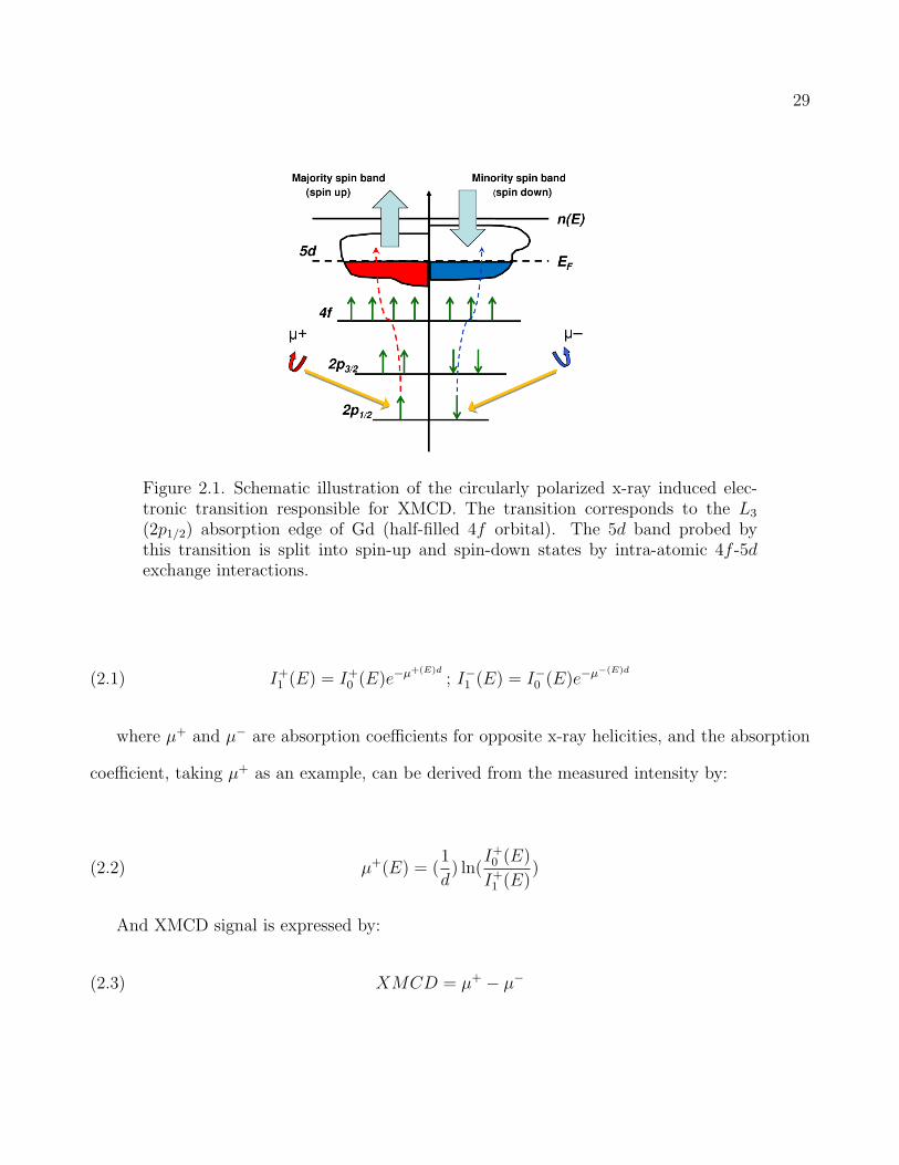
Figure 2.1. Schematic illustration of the circularly polarized x-ray induced elec-tronic transition responsible for XMCD. The transition corresponds to the L3
(2p1/2) absorption edge of Gd (half-filled 4f orbital). The 5d band probed bythis transition is split into spin-up and spin-down states by intra-atomic 4f -5dexchange interactions.
(2.1) I+1 (E) = I+
0 (E)e−µ+(E)d
; I−1 (E) = I−0 (E)e−µ−(E)d
where µ+ and µ− are absorption coefficients for opposite x-ray helicities, and the absorption
coefficient, taking µ+ as an example, can be derived from the measured intensity by:
(2.2) µ+(E) = (1
d) ln(
I+0 (E)
I+1 (E)
)
And XMCD signal is expressed by:
(2.3) XMCD = µ+ − µ−

30
0.00
0.05
0.10
0.15
0.20
0.700 0.705 0.710 0.715 0.720 0.725
-0.02
-0.01
0.00
0.01
L2
+
-
XA
S (
arb.
uni
ts) (a) L
3
+- -
(b)
XM
CD
(ar
b. u
nits
)
Energy (keV)
Figure 2.2. (a) helicity-dependent (µ+ and µ−) x-ray absorption spectra (XAS)and (b) XMCD (µ+-µ−) of L2 and L3 absorption edges for Fe+3 ions collectedfrom ε-Fe2O3 [50] samples.
The correlation between helicity-dependent absorption and XMCD spectra is illustrated in Fig.
2.2. XMCD has a major impact on understanding the element-specific physics of ferromagnetic
materials. By tuning the x-ray energy to selected atomic resonances, the measurements can yield
element- and orbital- selective magnetization [35].
Materials having ferromagnetic ordering are transition metals, rare earths and their alloys.
For transition metals (Ni, Co, Fe), their ferromagnetism is originated from unfilled 3d shells.
For rare earths, Gd or Tb for example, their ferromagnetic ordering is attributed to unpaired
electrons in unfilled 5d and localized 4f shells [36]. In rare earths, the 4f electron wave functions
are highly localized, and their ferromagnetic ordering is interpreted as the indirect exchange
between 4f electrons through the spin-polarized 5d (6s) conduction bands [36]. Unlike rare
earths, transition metals possess ferromagnetic ordering based on the direct exchange between

31
3d electrons. Thus, larger dichroic effects can be obtained at L2,3 -edges (2p → 3d) and M4,5
-edges (3d → 4f) in transition metals due to direct probe of 3d shell. Although probes of L2,3
-edges (2p → 5d) in rare earth also directly monitor the spin-polarization of the 5d shell, this
shell carries relatively smaller polarization that is induced by 4f shell. In this work, L3 -edge of
Gd was chosen because the XMCD signal at this particular energy can be detected in a diamond
anvil cell (DAC, described in Chapter 3).
The element- and orbital- selective advantages of XMCD are used in many areas ranging from
fundamental to applied aspects, such as magneto-electronics [37-40], earth sciences [41, 42]
and life sciences [43, 44]. In this work, XMCD was used at the Gd L3 -edge to probe 5d
polarization, which is proportional to 4f polarization and represents the magnetic properties
of Gd5(SixGe1−x)4. Si(Ge) K -edge (1s → 3(4)p) was also probed to understand how p states
mediate the FM interactions within the compounds. Although neutron diffraction is also capable
of probing magnetic structure, it was not used in this study because neutron diffraction requires
large sample size, which is not suitable for diamond anvil cell.
2.1.1. Sum rules calculations of XMCD
In addition to element- and orbital- selectivity, XMCD is also renowned for being capable
of decomposing spin (mspin) and orbital (morb) contributions to total magnetic moment. The
separation of mspin and morb is invaluable for understanding the fundamental origins of the
macroscopic magnetic properties of the matter. The decomposing process involves sum rule
calculations [45-47]. In the following, an example from the side-project of this thesis is given to
highlight this strength.

32
Example: magneto-crystalline anisotropic change in ε-Fe2O3 magnetic nanoparti-
cles
ε-Fe2O3 magnetic nanoparticles exhibiting a large coercivity field (Hc) of 20 kOe at room
temperature and bearing the characteristic of easy synthesis make it a potential candidate for
magnetic storage applications [48, 49]. However, a large reduction of Hc with temperature
decrease is obtained in this material, with a Hc of 0.8 kOe found at ∼ 110K (Fig. 2.3). XMCD
measurements were carried out and analyzed within the framework of sum rules to unveil this
magnetic softening characteristic. Details of sum rule calculations can be found in Ref. [47].
The 3d electron occupation number needed for a quantitative derivation of orbital and spin
components of magnetization, was set to n3d = 5 based on the 3d5 electronic configuration of
Fe+3 ions. The temperature-dependent mspin, morb, and morb/mspin quantities obtained from the
sum rule calculations are shown in Fig. 2.4.
The results show that mspin remains largely temperature independent while morb shows a
significant decrease around 120 K. In particular, the morb/mspin ratio, which is independent of
both the 3d electron configuration and the integration of XAS data, shows a significant reduction
(> 50 %) of the Fe 3d orbital moment at T ∼ 120 K and subsequently increases to attain at 80
K a value of the same order than the one measured at 200 K. It is argued [50] that the large
morb at room temperature is the origin of the moderately large anisotropy found in the material,
where the large reduction in morb at 120 K, and the related weakening of spin-orbital coupling,
is responsible for the decrease of the Hc around 110 K.

33
0 50 100 150 200 250 3000
5
10
15
20
25
Hc (
kO
e)
T (K)
-60 -40 -20 0 20 40 60-20
-15
-10
-5
0
5
10
15
20
T= 10 K
M (
em
u/g
)H (kOe)
-60 -40 -20 0 20 40 60-20
-15
-10
-5
0
5
10
15
20
T= 110 K
M (
em
u/g
)
H (kOe)-60 -40 -20 0 20 40 60
-20
-15
-10
-5
0
5
10
15
20
T= 260 K
M (
em
u/g
)
H (kOe)
Figure 2.3. Temperature dependence of the coercive field (Hc) for ε-Fe2O3 nanopar-ticles taken from [49]. The upper insets show the magnetization vs. magnetic fieldhysteresis loops of ε-Fe2O3 nanoparticles measured at 10 K, 110 K and 260 K,respectively

34
Figure 2.4. Temperature-dependence of the orbital (morb) and spin (mspin) effectivemoments and the ratio of orbital/spin (morb/mspin) for ε-Fe2O3 nanoparticles.
2.1.2. Vectorial characteristics of XMCD
It is also important to note that XMCD is a vectorial probe of magnetism. Since the photo-
electron is spin-polarized along or opposite the x-ray helicity, i.e., x-ray propagation direction, the
XMCD signal depends on the relative alignment of the x-ray wave-vector and the quantization
axis determined by an applied magnetic field, , where is the local moment direction (Fig. 2.5).
Since the x-ray absorption process averages over many absorbing sites, the vectorial nature of
XMCD implies that an element-specific magnetization is required to yield a XMCD signal 〈 ~K· ~M
6= 0〉. This allows XMCD to probe the net projection of moment aligned along the direction of
photon wave-vector.

35
M→
Figure 2.5. Schematic illustration of the vectorial-probe characteristic of XMCD.~K represents the x-ray photon wave-vector with helicity-dependency and ~M rep-resents the real magnetic moment. ~K· ~M is the effective magnetic moment probedby XMCD.
Example: interfacial magnetism in SrRuO3/SrMnO3 multilayer system
A multilayer system composed of perovskite SrRuO3 (SRO) and SrMnO3 (SMO) thin films
was investigated. SRO is a ferromagnet with Tc of ∼ 163 K [51] and strong out-of-plane
anisotropy. SMO is a G-type antiferromagnet with a Neel temperature (TN) of ∼ 260 K [52].
XMCD measurements were carried out with the magnetic field applied parallel to the x-ray prop-
agation direction, which is along the film normal [53, 54]. Since XMCD is proportional to the
net magnetic moment of resonant atoms projected along the x-ray propagation direction, it can
be seen in Fig. 2.6(a) that despite the AFM characteristic of SMO layer, the Mn ions possess
a net out-of-plane ferromagnetic moment with applied field (H) of 10 kOe at 50 K. However, as
the field increases to 40 kOe, the XMCD signal vanishes. This suggests that either the net Mn
moment disappears or rotates to the direction orthogonal to photon wave-vector, or could be

36
-0.004
-0.002
0.000
0.002
2840 2850 2860 2870 2880
0.000
0.006
0.012
0.018
635 640 645 650 655 660-2
0
2
4
2840 2850 2860 2870 2880-1
0
1
2
XAS XMCD 10 kOe XMCD 40 kOe
XAS XMCD 0 kOe XMCD 20 kOe XMCD 40 kOe
Energy (eV)
XM
CD
(arb. units)X
MC
D (arb. units)
XA
S (
arb.
uni
ts)
XA
S (
arb.
uni
ts)
(b)
(a)
Figure 2.6. Magnetic-field dependence (in kOe) of out-of-plane XMCD signals for(a) Mn L2, L3 -edges and (b) Ru L2 -edge at 50K. Ru L3 -edge was not probeddue to energy-range limitation at the beamline 4-ID-C, the Advanced PhotonSource.
both. The field-dependence of Ru moment at the same temperature is shown in Fig. 2.6(b). As
expected, a large out-of-plane Ru moment is observed. The remanent Ru moment obtained at H
= 0 is ∼ 70 % of that obtained at H = 40 kOe by comparing the XMCD signal, suggesting that
it results from the strong out-of-plane anisotropy of SRO layer. The reverse sign of XMCD be-
tween Mn and Ru moment upon field-dependence suggests an antiferromagnetic (AFM) coupling
between SRO and SMO layers, as shown in Fig. 2.7.

37
(a) H = 0 (b) H > 0
HOut-of-plane
Ru
Mn
Net Mn
Figure 2.7. Schematic illustration of the spin configuration of SRO/SMO multi-layer system with and without an out-of-plane applied field.

38
2.2. X-ray absorption fine structure (XAFS)
X-ray absorption fine structure (XAFS) is a powerful technique for studying local structure
in both ordered and disordered materials [55]. The spectroscopy acquires the energy range near
and above the core-level binding energy of the selected atom. XAFS can probe chemical and
physical states, sensitive to the coordination number, bonding distances surrounding around the
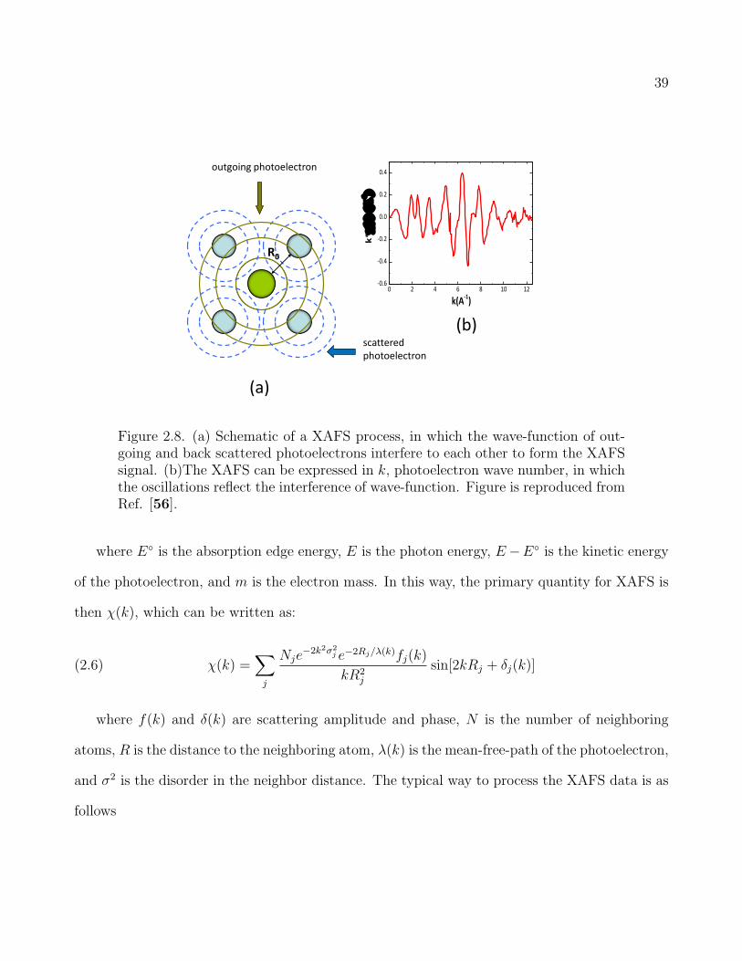
selected atoms. Fig. 2.8(a) is the sketch of XAFS process. An x-ray photon comes in and is
absorbed by the selected atom [56]. The absorption process liberates the core-level electron,
generating the outgoing photoelectron. The outgoing photoelectron leaves the absorbing atom
with a spherical wave until it hits the electron-cloud of the neighboring atoms. Hence, the
photoelectron is scattered by the neighboring atom and goes back to the absorbing atom. The
interference between the outgoing and back scattered wave-functions results in a modulation of
x-ray absorption coefficient, giving rise to the XAFS (Fig. 2.8(b)).
For XAFS, the interest is in the oscillations above the absorption edge, and define the XAFS
fine structure function χ(E) as:
(2.4) χ(E) =µ(E)− µ◦(E)
µ◦(E)
Here µ◦(E) is the absorption coefficient of an isolated atom, and µ(E) is the absorption coef-
ficient of the atom in the material of interest. χ(E) can be further expressed as a function of
photoelectron wave number, k, which has dimensions of 1/distance. Energy and wave number
are related by:
(2.5) k =
√2m(E − E◦)
~2
39
R0
outgoing photoelectron
scattered photoelectron
(a)
(b)
0 2 4 6 8 10 12-0.6
-0.4
-0.2
0.0
0.2
0.4
k(A-1
)
k*
Figure 2.8. (a) Schematic of a XAFS process, in which the wave-function of out-going and back scattered photoelectrons interfere to each other to form the XAFSsignal. (b)The XAFS can be expressed in k, photoelectron wave number, in whichthe oscillations reflect the interference of wave-function. Figure is reproduced fromRef. [56].
where E◦ is the absorption edge energy, E is the photon energy, E−E◦ is the kinetic energy
of the photoelectron, and m is the electron mass. In this way, the primary quantity for XAFS is
then χ(k), which can be written as:
(2.6) χ(k) =∑j
Nje−2k2σ2
j e−2Rj/λ(k)fj(k)
kR2j
sin[2kRj + δj(k)]
where f(k) and δ(k) are scattering amplitude and phase, N is the number of neighboring
atoms, R is the distance to the neighboring atom, λ(k) is the mean-free-path of the photoelectron,
and σ2 is the disorder in the neighbor distance. The typical way to process the XAFS data is as
follows

40
• Convert measured intensities to µ(E), and subtract a smooth pre-edge background from
µ(E) to get rid of absorption from other edges.
• Identify the threshold energy E◦, and normalize µ(E) to go from 0 to 1, so that it
represents the absorption of one atom.
• Remove a smooth post-edge background function to approximate µ◦(E).
• k-weight the XAFS χ(k) and Fourier transform into real space.
A typical XAFS analysis process is shown in Fig. 2.9 [57]. By comparing with theoretical
calculations, the XAFS data can be analyzed to obtain the local structure around the selected
element. In this work, XAFS was used to probe local contraction effect around Si atoms (Chapter
6) and to calibrate pressure (Chapter 3).

41
0
0 2 4 6 80.0
0.1
0.2
0.3
0.4
0.5
(d)
� (R)
(A-2)
R (A)
8900 9000 9100 9200 9300 9400 9500
0.0
0.2
0.4
0.6
0.8
1.0
1.2
1.4
(a)
� (E
)
E (eV)0 2 4 6 8 10 12
-0.2
-0.1
0.0
0.1
0.2
0.3
�� ��
k (A-1)
(b)
0 2 4 6 8 10 12-0.6
-0.4
-0.2
0.0
0.2
0.4
0.6
k*
�� ��� ��� �
k(A-1)
(c)
Figure 2.9. XAFS analysis process. (a) The raw XAFS spectrum is pre-edge sub-tracted to remove the background and then be normalized. (b) The normalizedspectrum is converted into k-space and (c) be k-weighted, and (d) finally be Fouriertransformed into real-space. Figure is reproduced from Ref. [58].

42
θ d
Incident beam reflected beam
θUpper plane
Lower plane
θ
dsinθ
Figure 2.10. Schematic illustration of the Bragg diffraction.
2.3. X-ray powder diffraction (XRD)
X-ray powder diffraction (XRD) is widely used to determine crystal structures based on their
diffraction patterns. In general, XRD could (1) determine the crystal structures of identified
materials and (2) identify single- or multi-phase conditions according to Bragg diffraction law:
(2.7) 2d sin θ = nλ
where d is the atomic interplanar spacing; θ is the diffraction angle; n is an integer; λ is the
wavelength of the x-ray. The angle of the diffraction is related to the atomic interplanar spacing
(Fig. 2.10) and the intensity of the diffraction peak depends on the exact positions of atoms in
the unit cell, which is the structure factor, and their disorder. The structure factor (F (Q)) and
its relationship to the x-ray intensity (I) can be expressed as:
(2.8) F (Q) =∑rj
Fmolj (Q)eiQ·rj

43
(2.9) I = |F (Q)|2
Here rj is the position of the jth molecule in the unit cell [58]. In this work, in order to obtain
the pressure-induced volume change (compressibility), XRD was collected in a diamond anvil
cell (Chapter 3) using the angle-dispersive setup at the sector 16 of the Advanced Photon Source
(Fig. 2.11).
As shown in Fig. 2.11, the diffraction patterns were collected using a MAR345 image plate
(pixel size 100 × 100 gm2. The collected two-dimensional diffraction rings on the image plate
(Fig. 2.12(a)) were integrated with FIT2D program [59] into diffraction pattern of intensity
versus 2θ (Fig. 2.12(b)). In this work, Rietveld refinement [60] was employed to determine
crystallographic structures, lattice parameters, and quantitative amounts of different phases in
pressure-induced multi-phase mixtures of the materials.

44
2D image plate Beam stopper
Figure 2.11. Angle-dispersive powder diffraction setup. Figure is taken from Ref. [61].

45
(a) (b)
5 10 15 20 25
0
5
10
15
2
Inte
nsi
ty x
10
00
(a
rb.
un
its)
Figure 2.12. (a) The diffraction pattern of Gd5(Si0.5Ge0.5)4 sample collected usinga 2-dimensional image plate and (b) integrated into an intensity vs 2θ diffractionpattern.

46
CHAPTER 3
High pressure experimental setup
3.1. High-pressure XMCD beamline setup
High-pressure XMCD measurements were carried out at beamline 4-ID-D of the Advanced
Photon Source, Argonne National Laboratory. The beamline setup is shown in Fig. 3.1. A 1×1
mm2 x-ray beam produced by a 2.4 m-long linear undulator insertion device is monochromized
by a Si (111) double-crystal monochromator [32, 33]. For XMCD measurements, the linearly
polarized x-rays are converted to circularly polarized by means of a C(111), 100 µm-thick diamond
crystal phase retarder (PR) optics [34]. Toroidal (Pd) and flat (Si) mirrors focus the x-ray beam
to ∼ 100×180 µm2 at the position of the slit before the sample. Harmonic rejection is critically
important during the measurements due to the significant attenuation of PR, diamond anvils
and the sample (100 ∼ 500 times at 7 keV), and the focusing mirror can provide a combined
harmonic rejection of ∼ 105 at 7 keV. Additional harmonic rejection can be achieved by detuning
the second Si (111) crystal of the monochromator away from its Bragg-peak as needed. A split
ion-chamber (IC) is used to monitor and maintain the vertical beam position by adjusting the
angular position of the second Si (111) crystal using a PZT and a feedback loop. The x-ray
beam size is further reduced to either (100×100) or (50×50) µm2 according to the aperture of
the perforated diamond anvils (will be discussed below).

47
Fig
ure
3.1.
Sch
emat
icillu
stra
tion
ofth
eex
per
imen
tal
hig
h-p
ress
ure
XM
CD
setu
pes
tablish
edat
bea
mline
4-ID
-Dof
the
Adva
nce
dP
hot
onSou
rce,
Arg
onne
Nat
ional
Lab
orat
ory.

48
IC1 and IC2 are used as detectors of incident and transmitted intensities, located before and
after the sample, respectively. The XMCD signal is collected by modulating the x-ray helicity at
11.7 Hz and detecting the related modulation in the absorption coefficient with a lock-in amplifier
[62].
A non-magnetic, piston-cylinder type copper-beryllium diamond anvil cell (DAC) manufac-
tured by easyLab Technology is mounted on a helium-flow cryostat with an extended cold-finger
(Fig. 3.2). The DAC reaches temperature as low as ∼ 9 K. The cryostat itself is mounted on high
resolution x, y translation stages for sample positioning with 1 µm accuracy, and placed between
the pole pieces of an electromagnet, which provides a maximum magnetic field strength of 0.7
Tesla at the sample position. The long-travel X-translation stage is used to move the sample in
and out of the electromagnet in order to do sample loading and in-situ pressure calibration using
the ruby fluorescence method. A Huber 410 goniometer allows a θ rotation of the cryostat/DAC
about the vertical axis. This allows to rotate the single crystalline diamond anvils away from
unwanted Bragg diffraction which otherwise gives rise to glitches in the absorption spectra.
3.2. Diamond anvil cell (DAC)
The Diamond anvil cell (DAC) is typically used for high pressure experiments. In a con-
ventional DAC, the material of interest is placed in the cell, in which the opposing force will
be applied through the backing plates to the anvils generating pressure on the sample located
in a cavity of a gasket. In this work, the absorption edge of interest is Gd L3 (7.243 keV). In
order to reduce diamond absorption at this particular edge, the diamonds were perforated. The
DAC consists of a fully perforated diamond anvil (FPA) which serves as a backing plate for a
mini-anvil (MA) 0.7 mm high, and an opposing, partially perforated anvil (PPA) with a 0.1 mm

49
GdSiGe
Cu
Ruby
Powder mixtureIn Si-oil (1:1:2 by weight)
Figure 3.2. Membrane-driven diamond anvil cell mounted on the cold finger exten-sion of a He-flow cryostat. A schematic of the asymmetric diamond anvil config-uration, including fully-perforated-, partially-perforated- and mini-anvil is shownin the inset. The sample mixture (described in text) is loaded into a drilled cavityof the pre-indented gasket.
inner wall. Paired 0.6 or 0.45 mm culets for the MA and PPA were used in the DAC depending
on the target pressure ranges. For 0.6 mm culet, pressure up to 16 GPa can be generated; for
0.45 mm culet, a maximum P of ∼ 23 GPa has been reached. The configuration of the DAC
is shown in Fig. 3.2 [63]. The asymmetric configuration of the DAC retains a smooth optical
surface on the mini-anvil side to allow in-situ ruby fluorescence pressure calibration. The rough
inner surface of the partial conical perforation scatters strongly the optical fluorescent photons
and reduces the intensity.
Unlike a strain-gauge pressure cell whose pressure needs to be increased ex-situ by a knob
and then to be read via a transducer, pressure is changed in-situ in our DAC by controlling

50
the He-gas pressure in an expanding membrane which drives the piston motion of the cell. The
He-gas pressure can be adjusted remotely by a pressure-control-box connected to a He cylinder
bottle. The advantage of this setup is no need for warming up the cryostat for removing the
DAC. While the disadvantage is that the sizable DAC inevitably limits the minimum gap of the
electromagnet hence reducing the strength of the magnetic field.
3.3. Sample preparation
The sample preparation requires three elements− pressure medium (Si-oil), pressure calibrant
(Cu or ruby powders), and the material of interest (Gd5(SixGe1−x)4 compounds), as shown in
Fig. 3.2. The samples used in measurements require very fine powders size, usually less than
1 µm in diameter. If the pressure calibrant is Cu, the mixture of the sample follows a weight
ratio of 1:1:2 for Gd5(SixGe1−x)4, Cu powders and silicon-oil, respectively in order to yield an
ideal absorption jump of ∼ 1 for both Gd L3 and Cu K -edges. If the pressure calibrant is
ruby, its powders need to be homogeneously coated on the surface of the MA without mixing
with Gd5(SixGe1−x)4 and silicon-oil. This allows the emitted ruby fluorescence to be collected
efficiently through the perforation of the FPA. The sample mixed with Cu calibrant if needed is
then loaded into a 250 µm hole in a nonmagnetic stainless steel gasket, which was pre-indented
down to a thickness range of 80 - 60 µm depending on the target pressure range.
3.4. Pressure calibration
Two in-situ pressure calibration methods, Cu XAFS and ruby fluorescence have been used
in this work for different considerations. In the beginning, Cu XAFS was used due to the un-
availability of ruby-fluorescence optical system. However, this method requires energy switching
between different absorption edges (Gd L3 and Cu K -edges) and extended energy XAFS scans
51
through the absorption edge of the calibrant material, which is very time consuming. Another
disadvantage of the Cu XAFS is that its absolute accuracy is about 0.5 - 1 GPa, poorer than
∼ 0.1 GPa acquired in the ruby fluorescence method. The relative change in pressure can be
determined with much better accuracy of ∼ 0.1 GPa. In addition, Cu XAFS is easily affected
by Bragg diffraction induced by the single crystalline diamond anvils which heavily worsens the
calibration results. The advantage of the Cu XAFS is that a smooth optical surface of a diamond
anvil required in ruby fluorescence method is not necessary, which reduces the cost of diamond
anvils. In general, pressure calibration using Cu XAFS is useful when optical access to the DAC
is not feasible. The reason why XRD was not used as a pressure calibration method in this
work is because it requires a CCD camera (described in Chapter 2) which is not the standard
apparatus in 4-ID-D beamline.
3.4.1. Cu XAFS pressure calibration
In-situ pressure calibration using x-ray absorption fine structure measurements can be traced
to Ref. [55, 64]. Copper is suitable for this method as it has a cubic structure and a known
compressibility [65]. In addition, its K absorption edge (8.979 keV) is in close proximity to
the energy of the wanted measurements (Gd L3 is 7.243 keV). Since XAFS can probe the local
structure of the selected atom (described in chapter 2), it can, therefore, determine the pressure
by comparing the bond-length changes against the known compressibility of the calibrant. Fig.
3.3(a) shows raw absorption spectra of CuK -edge for different pressures. The data were collected
from a reference Cu powder sample (< 1µm), outside (ambient condition) and inside the DAC
(2.4 and 9.8 GPa) respectively. It is known that the phase of the XAFS signal depends on
inter-atomic distances through

52
(3.1) χ(k) ≈ sin[2kRj + δj(k)]
where Rj is the bonding length and δj is the scattering phase shift. A volume reduction
would result in a reduction of the photoelectron phase 2kR and an elongation outwards of the
k-dependent XAFS oscillations, as shown in the inset of Fig. 3.3(a). The changes in inter-atomic
distance with pressure can also be clearly seen in the Fourier transform (FT) of the XAFS as
shown in Fig. 3.3(b). The fitting model used FEFF 6.0 standards [66] and IFEFFIT 2.8 package
[67], assuming a uniform compressibility of all Cu-Cu bonds, and the real space fits include
contributions from the first two atomic shells only.

53
Figure 3.3. (a) Raw Cu K-edge absorption spectra measured at different pressures.Inset shows the background-removed XAFS data.(b) Magnitude (main panel) andreal part (inset) of the complex Fourier transform of XAFS data together withrepresentative fits. (c) Pressure calibration using the volume reduction measuredby XAFS (empty squares) and the compressibility of Cu at 300 K (red curve).Pressure calibration from ruby fluorescence is also shown (filled squares)

54
In addition to the decrease in inter-atomic distance, the amplitude increase of the FT is also
evident as a result of the decrease of bond-length vibrational disorder upon volume reduction.
The pressure was obtained by interpolating the fitted volume change (∆V) into the known
compressibility curve of Cu at 300 K. The fitted volume change can be expressed as
(3.2) ∆V/V◦ = 3×∆R/R◦
where ∆R is the change of bond-length. The pressures obtained from the fitted Cu XAFS
were compared with those gained from ex-situ ruby pressure calibration, as shown in Fig. 3.3(c).
3.4.2. Ruby fluorescence pressure calibration
Ruby fluorescence, which is the most widely used pressure calibration method in high-pressure
research [68] was employed in this work. This method utilizes the spectral shift of the ruby (α-
Al2O3 contains Cr+3) fluorescence R lines (R1 and R2) with the variation of external stress
(pressure) [69] as shown in Fig. 3.4. It is important to note that the peak positions of R1 and
R2 will shift with temperature change. In order to account for both pressure- and temperature-
dependent shifts of the spectra during the calibrations, a program consulting the fitting formulas
reported in Ref. [70] was used. The most accurate way to calibrate the pressure is to take
the average of two R lines. However, because of the weak intensity of R2 at low temperature,
only R1 was used for calibration during low temperature measurements. The reported pressure
values using ruby fluorescence in this work were the average of that obtained at the lowest
temperature (∼ 9 to 17 K) and room temperature (300 K), the difference being usually smaller
than ∼ 1.5 GPa. The spectra were taken from a portable ruby fluorescence system manufactured

55
��� ��� ��� ��� ��� ��� ��� ��� ��� ��� ��� ��� �������������������������������������������
Figure 3.4. Pressure-dependent ruby R-line fluorescence spectra taken at room temperature
by Optipress (now easyLab). Pressure was calibrated by translating the cryostat/DAC into the
ruby fluorescence station on the side of the electromagnet, as shown in Fig. 3.5 [71].

56
Figure 3.5. Portable ruby fluorescence detector assembled to a translation stagenearby the electromagnet and cryostat.

57
CHAPTER 4
Role of Si-doping in enhancing ferromagnetic interactions in
Gd5(SixGe1−x)4 compounds
4.1. Introduction
According to the phase diagram of Gd5(SixGe1−x)4 [13], in the compositional range 0.24 ≤
x ≤ 0.5, the giant MCE is related to a 1st order, magnetic-crystallographic phase transition, in
which a PM→ FM transition on cooling is accompanied by a change in crystal structure from a
M to O(I) phase [18, 19]. The Ge-rich alloys (0 ≤ x ≤ 0.2), on the other hand, exhibit two phase
transitions on cooling: a 2nd order PM → AFM transition and a 1st AFM → FM transition at
lower temperatures. This second transition is accompanied by a structural transition between
two orthorhombic polymorphs, i.e. between the so-called O(II)-type structure and O(I) [20].
The most notable feature of these phase transitions is the reversible breaking and reforming of
covalent Si(Ge)-Si(Ge) bonds connecting Gd-containing slabs, which occurs concomitantly with
the change of magnetic state. The crystal structure changes via a martensitic-like mechanism,
involving large shear displacement (∼ 0.5 A) of sub-nanometer-thick Gd-containing slabs [18, 19].
Since this reversible phase transition can be manipulated by application of a magnetic field,
most investigations [18-21] of the MCE in these materials have been carried out within the
compositional range for 0.24 ≤ x ≤ 0.5. In particular, Gd5(SixGe1−x)4 is the most (heavily)
studied, because its magneto-structural transition occurs near room temperature [18-21].

58
Although for Ge-rich (0 ≤ x ≤ 0.2) and middle range (0.24 ≤ x ≤ 0.5) compositions the
material is characterized by different magnetic-crystallographic phases, the FM ordering tem-
perature, Tc, is linearly dependent on Si content. For example, for the three compositions x =
0.125, 0.375 and 0.5 discussed in this chapter, Tc of 80 (3), 190 (5) and 275 (3) K, respectively,
are obtained [72, 73]. As addressed in Chapter 1, since Si and Ge atoms have markedly different
sizes, the unit cell volume is affected by the Si/Ge ratio. Similarly, hydrostatic pressure (P) has
been used to alter the unit cell volume, and dTc/dP of ∼ 3.0 K kbar−1 has been reported for the
0 ≤ x ≤ 0.5 range [28]. The goal of this work is to extend the pressure range up to ∼ 18 GPa in
order to better explore the correlation between Si doping-induced chemical pressure and applied
pressure upon the magnetic transitions. In addition, XAFS measurements of the Ge and Si local
structure were carried out in order to understand the effect of local lattice distortion around Si
dopants. These will be discussed in Chapter 6.
4.2. Experiment
Polycrystalline samples of Gd5(SixGe1−x)4 for x = 0.125, 0.375 and 0.5 were prepared as
described by Pecharsky and Gschneidner [18]. In addition, the alloys were heat treated at 1300
◦C for 1 hour. Fine powders (≤ 1 µm) of Gd5(SixGe1−x)4 were thoroughly mixed with fine
powders (≤ 1 µm) of Cu and dispersed in silicon oil which was used as hydrostatic pressure
medium. The sample preparation followed the recipe described in Chapter 3, and the in situ
pressure calibration was done by measuring Cu XAFS as described in the same chapter. High-
quality transmission x-ray data were collected over the Gd L3 (7.243 keV) and Cu K (8.979
keV) -edges through perforated anvils in the DAC. Gd L3 (7.243 keV) edge was probed under
an applied field strength of ∼ 0.7 Tesla.

59
4.3. Results for Gd5(Si0.125Ge0.875)4 and Gd5(Si0.5Ge0.5)4 compounds
The pressure dependence of the magnetic transition was measured in the 0.25 - 14.55 GPa
range for x = 0.125 and x = 0.5 samples. Figure 4.1 shows temperature-dependent Gd L3 -edge
XMCD data for the x = 0.125 sample at applied pressure of 0.25 GPa (Fig. 4.1(a)) and 14.55
GPa (Fig. 4.1 (b)). The inset figures show that the XMCD signal fully reverses upon reversal
of a 0.7 Tesla applied field as expected. The XMCD signal does not change significantly from
20 to 80 K, but drops quickly at 90 (3) K. This drop is due to the magneto-structural, 1st order
phase transition, which at ambient pressure occurs at 80 (3) K [23] as confirmed with XMCD
measurements outside the DAC [73]. At P = 14.55 GPa the magnetic transition has significantly
shifted upward in temperature.
Figure 4.2(a) and (b) show the integrated area under the XMCD curves for x = 0.125 and 0.5,
respectively, both normalized to the low-temperature saturation value as a function of temper-
ature for different applied pressures. The data show that the magnetic transition temperature,
Tc, is enhanced with pressure in both samples. It changes from 80 (3) K at ambient pressure to
257 (5) K at P = 14.55 GPa for x = 0.125, and from 275 (3) K at ambient to 336 (5) K at P =
10 GPa for x = 0.5.

60
7.22 7.23 7.24 7.25 7.26 7.27 7.28-4
-3
-2
-1
0
Ab
so
rptio
n (a
rb. u
ntis
)
P = 14.55 GPa
7.22 7.23 7.24 7.25 7.26 7.27 7.28
-2
-1
0
1
2
T = 20 K
XM
CD
(arb
. u
nit
s)
Energy (keV)
+0.7 Tesla -0.7 Tesla
XM
CD
(a
rb.
un
tis)
Energy (keV)
T(K) 20 80 100 150 200 240 260 280
(b)
7.22 7.23 7.24 7.25 7.26 7.27 7.28-4
-3
-2
-1
0
Ab
so
rptio
n (a
rb. u
ntis
)
7.22 7.23 7.24 7.25 7.26 7.27 7.28
-2
-1
0
1
2
XM
CD
(arb
. u
nit
s)
Energy (keV)
+0.7 Tesla -0.7 Tesla
T = 20 K
(a)
XM
CD
(a
rb.
un
tis)
Energy (keV)
T(K) 20 60 80 90 100 110 120 130 140
P = 0.25 GPa
Figure 4.1. Gd L3 -edge XMCD signal (normalized to the absorption edge jump)as a function of temperature for (a) P = 0.25 GPa and (b) P = 14.55 GPa, for x =0.125 sample. The insets show the reversal of XMCD signal upon reversal of ap-plied magnetic field. The helicity-independent absorption spectra, obtained as theaverage of absorption spectra for opposite helicities, is shown by the dashed lines.The sample thickness decreases with pressure causing a reduction in absorptionedge jump.

61
40 80 120 160 200 240 2800.0
0.2
0.4
0.6
0.8
1.0
M(T
)/M
S
Temp (K)
0.25 GPa 1.36 GPa 2.75 GPa 3.86 GPa 14.55 GPa
(a)
100 150 200 250 300 3500.0
0.2
0.4
0.6
0.8
1.0
ambient 2.4 GPa 9.8 GPa
(b)
M(T
)/M
S
Temp (K)
Figure 4.2. Integrated XMCD as a function of temperature for different appliedpressures for (a) x = 0.125 and (b) x = 0.5 samples. The XMCD signal is normal-ized to the saturation value at 20 K. The lines are guides to the eye. Error barsshown for P = 14.55 GPa data in (a) are the same for the other data sets.
Here, Tc is determined from the maximum absolute value of the derivative of the fitted lines.
Another notable feature of the data for x = 0.125 sample is the presence of a non-zero XMCD
signal above Tc for P = 0.25, 1.36, 2.75, 3.86 GPa, which is related to the AFM phase present
in the low-x region (x ≤ 0.2), whereas this feature is not observed at 14 GPa in this sample, or
at any pressure in the x = 0.5 sample.
The pressure dependence of Tc for x = 0.125 and x = 0.5 is summarized in Figs. 4.3 (a) and
(b), respectively. The dependence of Tc on x (ambient pressure) is superimposed to highlight
the correspondence between x and P.

62
0 2 4 6 8 10 12 14 160
50
100
150
200
250
300
350
0.15 0.20 0.25 0.30 0.35 0.40 0.45
0 2 4 6 8 100
50
100
150
200
250
300
350
0.80 0.85 0.90 0.95 1.00
x (Si)
x=0.125 outside cell x=0.125 inside cell
(a) x = 0.125
FMAFM
PMPM
Tem
p (K
)
Pressure (GPa)
x=0.5 outside cell x=0.5 inside cell Fit
(b) x = 0.5
PM
FM
0.5
Figure 4.3. Magnetic phase diagram as a function of Si concentration (top) andapplied pressure (bottom). The points indicate the observed Curie temperatures,Tc, for different pressures as measured by XMCD for (a) x = 0.125 and (b) x =0.5 samples. The ”outside cell” data correspond to ambient pressure condition.

63
The overlaying x scale is determined by using known Tc(x) values from the literature [25]
for x = 0.125, x = 0.5 and x = 1.0 at P = 0. One can see that the general features of Tc(x)
are also present in Tc(P), namely a linear dependence of Tc on P, with a change in slope at x ∼
0.5. As we discuss below, an additional common feature is the disappearance of the FM-AFM
transition on warming for P > 4 GPa, which manifests itself in the XMCD data as a non-zero
XMCD signal above Tc.
4.4. Discussions for Gd5(Si0.125Ge0.875)4 and Gd5(Si0.5Ge0.5)4
The non-zero XMCD signal above Tc for P < 4 GPa in Fig. 4.2(a) indicates the presence
of a small ferromagnetic component. Non-zero magnetization above Tc with a similar ratio of
Ms/Mtail ∼ 5.5 was also observed in the SQUID data of Morellon et al. [23] for an x = 0.1 com-
pound. The low-x, Ge-rich compounds are known to undergo a FM-AFM transition at ambient
pressure before they become paramagnetic at higher temperature. This intermediate transition
is only observed for x ≤ 0.2, while higher x samples directly transform into a paramagnetic phase
on warming [14, 18, 25]. The non-zero XMCD tail for T > Tc is likely due to canting of the
AFM structure induced by the 0.7 T applied field. For example, Gd5Ge4, which is AFM at zero
field displays significant canting in an applied field [74]. The non-zero XMCD tail is not present
in the P = 14.55 GPa data, indicating a direct transition from FM to PM state at this pressure.
The presence of a tail for P < 4 GPa (which in Fig. 4.3 (a) is shown to be equivalent to x < 0.22)
and its absence at P = 14.55 GPa (equivalent to x ∼ 0.43) is in agreement with the occurrence of
the FM-AFM transition only at low x (low pressure) and its absence at high x (high pressure).
The P (x)-T phase diagram shown in Fig. 4.3 highlights the pressure−Si correspondence.
Starting with x = 0.125 sample, pressures of P = 0.25, 1.36, 2.75, 3.86 and 14.55 GPa produce a

64
temperature-dependent magnetization corresponding to x = 0.14, 0.15, 0.17, 0.22 and 0.44, re-
spectively, resulting in ∆(Si%)/∆P = 0.205 (Si%) kbar−1 (Fig. 4.3(a)). The pressure dependence
of the magnetic transition temperature, Tc, is linear with a slope dTc/dP = 1.2 K kbar−1. For
comparison, a value of dTc/dP = 3.0 K kbar−1 was obtained in Ref. [28] for a limited pressure
range below 1.0 GPa.
The XMCD data measured on the x = 0.125 sample outside the DAC at ambient pressure [73]
show a Curie temperature of 80 K, which is in agreement with previous SQUID measurements
[14, 23] and also very close to Tc = 84 K found by a linear extrapolation to P = 0 of the data in
Fig. 4.3(a). At the other end of the x scale in this panel, a Tc of 284 K is found by extrapolating
the fit to x = 0.5, which is 9 K higher than 275 K directly measured in x = 0.5 sample at ambient
pressure [73] (represented by the filled square in Fig. 4.3 (b)).
The data shown in Fig. 4.3 (b) correspond to measurements performed on an x = 0.5 sample.
Applied pressures of P = 2.4 and 10 GPa result in Tc of 321 (5) and 336 (5) K, corresponding
to the x values of 0.8 and 1.0, respectively [14, 18, 25]. Interestingly, x = 0.5 sample at an
applied pressure of 10 GPa shows the same magnetic ordering temperature as pure Gd5Si4 with
Tc = 336 K. In addition, even though a Tc of 336 (5) K is the ultimate transition temperature
achieved by doping Si up to x = 1.0 sample, the data indicate that further increases in transition
temperature are expected for pressures beyond 10 GPa. This means that hydrostatic pressure
provides an additional flexibility in manipulating Tc than Si doping does (albeit in a reversible
way), because it is not limited by the end boundaries of the solid solution.
At ambient pressure, the x = 0.5 sample is located near a structural boundary. While
it is monoclinic (M) at room temperature, a slight increase in Si concentration drives it into
the orthorhombic (O(I)) phase with a concomitant increase in Tc. Since the compressibility

65
of monoclinic and orthorhombic phases are markedly different [75], this structural transition is
responsible for the observed discontinuity in dTc/dx at x ≤ 0.5 [14, 18, 25]. Similarly, pressure
causes a 1st order M → O(I) transition in x = 0.5 sample within a range of P ∼ 1.0−2.0 GPa
[26], with Tc changing from 275 to 305 K. Here the smallest pressure of P = 2.5 GPa is large
enough to cause the transition into the O(I) phase, and this transition with its related Tc increase
is responsible for the discontinuity in dTc/dP . The slope of a fit through P = 2.4, 10 GPa data
points yields a dTc/dP = 0.2 K kbar−1, which is lower than the 0.9 K kbar−1 reported in Ref.
[76]. The correspondence between doping and pressure using the x = 0.5 data is ∆(Si%)/∆P
= 0.26 (Si%) kbar−1, which is comparable to 0.205 (Si%) kbar−1 obtained using the x = 0.125
data in Fig. 4.3(a).
The results clearly demonstrate that the FM → PM transition in Gd5(SixGe1−x)4 alloys is
similarly affected by Si doping and applied pressure at least in a qualitative way. Magnetic
interactions between localized Gd 4f moments are indirect since there is virtually no overlap
between Gd 4f wave-functions. Most intermetallic alloys exhibit an indirect Ruderman-Kittel-
Kasuya-Yosida (RKKY) [77] coupling through a spin-polarized conduction band. While this is
likely the dominant mechanism for exchange coupling between Gd ions inside Gd-slabs (intra-
slab), it has also been argued [14] that an indirect super-exchange coupling [78] plays a role in
mediating inter-slab coupling through the intervening, non-magnetic Si(Ge)-Si(Ge) bonds that
connect the Gd slabs in the FM, orthorhombic structure. The recent observation of magnetic
polarization in Ge 4p orbital due to hybridization with Gd 5d orbital, however, indicates that
RKKY coupling may also be involved in mediating the inter-layer magnetic coupling [73].
Regardless of whether the inter-slab coupling is of RKKY or superexchange type, its strength
is intimately connected with the overlap of Gd 5d and Si 3p (Ge 4p) states. This overlap is

66
enhanced by a volume contraction induced by either Si doping or applied pressure. For super-
exchange interactions, the increased overlap of magnetic Gd 5d and non-magnetic Si 3p (Ge 4p)
states increases the probability for virtual hopping needed to mediate Gd-Gd indirect exchange.
For RKKY interactions, the increased overlap between Gd 5d-Si 3p (Ge 4p) states promotes
hybridization and the related ability to transfer magnetic interactions through a spin-polarized
Gd 5d-Si 3p (Ge 4p) conduction band.
Prior to this study, unambiguously distinguishing between the effects of volume reduction,
Si(Ge) site occupancy and changes in electronic structure introduced by Si doping upon the
magnetic properties of these materials was difficult. Since the related work done by Morellon
et.al [28] has revealed that volume contraction affects both electronic and crystal structures in a
low pressure range (< 1 GPa), the equivalency between x and P in an extended pressure range
shown in this work has demonstrates that the application of pressure in an extended range is
able to reproduce all of the features in the x-T magnetic phase diagram. This may be interpreted
as an indication that, at least qualitatively, volume-driven effects can account for the observed
Si-induced changes in the x-T magnetic phase diagram.
However, evaluating the quantity where is the fractional change in volume-induced by pressure
by pressure or doping, provides a measure of the efficiency by which a structural volume change is
converted into a change in Tc. Using the compressibility value of κ = -0.25 Mbar−1 in Ref. [27],
and the doping-dependent lattice parameters in [18], it is found that Si-doping is more effective
in increasing Tc than pressure is for a given volume change. This indicates that Si-doping does
more to stabilize ferromagnetic interactions than simply uniformly reducing the volume of the
unit cell. A more detailed study for this aspect is presented in Chapter 6.

67
4.5. Results and discussions for Gd5(Si0.375Ge0.625)4
Due to a limited pressure range attained in above experiments (≤ 15 GPa) [79], two different
compounds, namely x = 0.125 and x = 0.5 were needed in order to fully explore the corre-
spondence of pressure and chemical Si doping over the entire 0 < x ≤ 1.0 range. In particular,
we were not able to directly demonstrate that the observed discontinuity in Tc(x) at x = 0.5
[25] is volume-driven. Therefore, a x = 0.375 sample with Si content between those of the two
previously studied samples (x = 0.125 and x = 0.5) was measured. This allowed us to directly
prove that the discontinuity in Tc(x) at x ∼ 0.5 is volume driven and also to further establish
the correspondence between Si doping (chemical pressure) and physical pressure in this class of
giant magnetocaloric effect compounds. The Tc of x = 0.375 increases with pressure, as was also
observed for both x = 0.125 and x = 0.5 samples. The magnetic transition temperatures as a
function of pressure for x = 0.125, x = 0.375, and x = 0.5 samples are presented in Fig. 4.4(a).
It is easy to see that the sample with x = 0.125 yields a linear dTc/dP up to ∼ 15 GPa, while
that with x = 0.375 exhibits a discontinuity in dTc/dP at ∼ 7.2 GPa. A similar discontinuity
induced by pressure was also observed for x = 0.5 [26, 76, 79]. It is known that a β (M) →
α (O(I)) phase transition is responsible for this discontinuity in Tc for x = 0.5 as a result of
the different compressibilities of M and O(I) structures [26]. Since the discontinuity in dTc/dP
occurs at ∼ 277 K on both x = 0.375 and x = 0.5 samples, it is reasonable to assume that the
M → O(I) structural transition for x = 0.375 occurs at ∼ 7.2 GPa at Tc of 277 (5) K (see the
dashed line in Fig. 4.4(a)). In addition, the dTc/dP for x = 0.375 at pressures below 7.2 GPa
in Fig. 4.4 (a) is 1.5 K kbar−1, which is comparable to 1.2 K kbar−1 obtained in x = 0.125.
Furthermore, dTc/dP measured at higher pressures reduces to 0.15 K kbar−1, comparable to 0.2
K kbar−1 obtained for the x = 0.5 sample. The good quantitative similarities reveal that x =

68
0 2 4 6 8 10 12 14 16 18 20
100
150
200
250
300
350
0 2 4 6 8 10 12 14 16 18 20180
200
220
240
260
280
300
320
340
TC (
K)
, x = 0.125, x = 0.375, x = 0.5
TC (
K)
277K
(a)
PM(M)
(b)FM(O(I))
FM(O(I))
PM(O(I))
Pressure (GPa)
Figure 4.4. (a) The transition temperature as a function of pressure of x = 0.125,0.375, and x = 0.5 samples, respectively. Open symbols represent the data mea-sured at ambient conditions. The horizontal dashed line marks slope discontinuityobserved for the x = 0.375 sample, and the Tc (277K) of x = 0.5 under ambientconditions. (b) The P − T phase diagram of x = 0.375. The data points indicatethe transition temperatures under different pressures. The transition regime ismarked by dashed lines located between 7.18 and 8.1 GPa .
0.375 behaves analogously to x = 0.125 at low pressures and to x = 0.5 at high pressures. This
behavior is dictated by the change in compressibility introduced by the M → O(I) structural
transition.
A P -T diagram is plotted in Fig. 4.4 (b) [72] for the x = 0.375 sample. The discontinuity in
dTc/dP at 277 K is also observed at this temperature in the x-T phase diagram, where the M→
O(I) structural transition occurs at x ∼ 0.5 [25]. Hence, our results indicate that this transition
is volume driven. When the volume reduction causes Tc to reach 277 K, a low-Si/low-pressure
phase (monoclinic) will be converted into a high-Si/high-pressure phase (O(I)).

69
4.6. Conclusion
Using XMCD we have demonstrated that applying hydrostatic pressure yields similar, quali-
tative magnetic behavior to that obtained by Si-doping in Gd5(SixGe1−x)4 (x = 0.125, 0.375, 0.5)
over a large pressure range up to ∼ 18 GPa. This correspondence is quantified to be 0.233 (Si%)
kbar−1. All features in the x-T magnetic phase diagram of these materials are also reproduced by
applying pressure, namely, the disappearance of the intermediate AFM phase, a linear increase
in Tc and a discontinuity in dTc/dP at Tc of 275 K. Based on the reported compressibility and
doping-dependent lattice parameters for these compounds, our results indicate that Si-doping
does more to stabilize FM interactions in these materials than is achieved by an uniform reduc-
tion in lattice volume alone. This quantitative difference between pressure and Si-doping will be
fully addressed in Chapter 6.

70
CHAPTER 5
Emergence of ferromagnetic order from within antiferromagnetic
phase of Gd5Ge4: pressure studies of low-x region
5.1. Introduction
In general, the ferromagnetic nature of Gd5(SixGe1−x)4 for x ≥ 0.2 is well established [14, 18].
However, the low-x region of the phase diagram is less understood. In this region an intermediate
AFM phase is observed for x < 0.2 in the 30−130 K temperature range, intermediate to FM (T
< 80 K) and PM (T > 130 K) phases (see phase diagram in Fig. 1.5). The presence of this AFM
phase at low x and intermediate temperatures, displaying AFM coupling between Gd ions across
slabs but FM coupling within the slabs [76], is indicative of the close proximity in total energy
between FM and AFM phases in the low x region of the phase diagram [80]. A contraction of
the lattice, either through Si-doping or applied pressure, enhances the inter-slab FM interactions
and stabilizes FM ordering. For example, the ground state of pure Gd5Ge4 is AFM-O(II) phase,
and pressure converts it into FM-O(I) phase [29]. However, the mechanism leading to the
emergence of FM-O(I) phase from within the AFM-O(II) phase of the parent Gd5Ge4 compound
at low x is still a matter of debate. In particular, the question arises whether the low-x samples
should be described as AFM-O(II)/FM-O(I) mixtures, or otherwise as structurally homogeneous,
ternary solid-solutions where competing FM and AFM interactions are simultaneously present
[31]. Because of the strong electron-lattice coupling present in these compounds, both scenarios
are expected to result in an inhomogeneous magneto-structural ground state. This inhomogeneity

71
could in principle be removed by expanding the lattice volume, which favors an AFM phase, or
by contracting the lattice with external pressure or chemical pressure (Si-doping), which favors
the FM state [25, 28, 79, 80].
In this chapter we present evidence from x-ray diffraction, temperature-dependent bulk mag-
netization measurements, and x-ray magnetic circular dichroism measurements at ambient- and
high-pressure conditions indicating that the magnetism of low-x samples (0 < x ≤ 0.075) is
characterized by the simultaneous presence of the AFM-O(II) and FM-O(I) phases, their volume
fractions depending not only on Si content, x, but also on applied pressure and magnetic field.
The application of pressure reduces the lattice volume and stabilizes the FM-O(I) phase, leading
to a magnetically- and structurally- homogeneous ground state where ordered magnetic moments
typical of high x samples are recovered.
5.2. Experiment
Polycrystalline samples of Gd5(SixGe1−x)4 with x = 0, 0.025, 0.05, 0.075, 0.125 and 0.5 were
prepared at Ames Laboratory. The samples were heat-treated at 1300 ◦C for 1 hour to achieve
homogeneous atomic distribution, and then were finely ground into micron-sized powders. X-ray
diffraction patterns were collected on a Rigaku TTRAX rotating anode powder diffractometer
using Mo Kα radiation and fitted by Rietveld refinement (by Ya. Mudryk at Ames lab). The x-
ray powder diffraction measurements at temperatures from 10 K to 300 K and in magnetic fields
from 0 to 30 kOe were performed on the same diffractometer equipped with a continuous flow
helium cryostat and a superconducting magnet [81]. Room temperature results show a linear
dependence of the lattice parameters on Si content, indicating that Si incorporates into the lattice
(Fig. 5.1). Superconducting Quantum Interference Device (SQUID, Quantum Design MPMS

72
0.000 0.025 0.050 0.075 0.100 0.1257.688
7.692
7.696
7.700
0.000 0.025 0.050 0.075 0.100 0.125
14.826
14.829
14.832
14.835
0.000 0.025 0.050 0.075 0.100 0.1257.775
7.780
7.785
7.790
0.000 0.025 0.050 0.075 0.100 0.125886
887
888
889
890
a (Å
)
b (Å
)
c (Å
)
x (Si)
volu
me
(Å3 )
Figure 5.1. Lattice parameters and unit-cell volume of Gd5(SixGe1−x)4 compoundsat room temperature as a function of Si content. All samples exhibit the O(II)-typestructure at ambient conditions.
XL-7) measurements of the dc magnetic susceptibility in a 50 Oe applied field (at Northwestern
University), both for field-cooling (FC) and zero-field cooling (ZFC), show that all samples display
ferromagnetic transitions with Tc values of 32, 46, 58, 80, and 275 K for x = 0.025, 0.05, 0.075,
0.125 and 0.5 respectively (Fig. 5.2). In this chapter results from only x = 0.025, 0.05, and
0.075 samples are presented since high-x samples were already described in Chapter 4. Other
experimental details related to the high-pressure XMCD measurements are also as described in
Chapter 4.

73
50 100 150 200 250 300 3500.0
0.5
1.0
1.5
2.0
2.5
50 100 150 200 250 300 3500.0
0.5
1.0
1.5
2.0
2.5
0.025 (ZFC) 0.025 (FC) 0.05 (ZFC) 0.05 (FC) 0.075 (ZFC) 0.05 (FC) 0.125 (ZFC) 0.125 (FC) 0.5 (ZFC) 0.5 (FC)
Mag
netiz
atio
n (e
mu/
g)
Temp (K)
H = 50 Oe
Figure 5.2. Temperature-dependent dc magnetization data of Gd5(SixGe1−x)4 com-pounds for x = 0.025, 0.05, 0.075, 0.125, and 0.5 samples measured on warming ina H = 50 Oe applied field after field (FC) and zero-field cooling (ZFC).
5.3. Results
The lattice parameters (a, b, and c) and unit cell volume as a function of x are plotted
in Fig. 5.1. All samples have a PM-O(II) phase at room temperature. Fig. 5.2 shows the
temperature-dependent FC and ZFC SQUID magnetization data measured on warming for low-
x (0.025, 0.05, 0.075) and higher-x (0.125, 0.5) samples. According to the Gd5Si4 − Gd5Ge4
phase diagram (Fig. 1.5), the lowest temperature transition found in x = 0.025, 0.05, 0.075,
and 0.125 samples on warming is FM → AFM, and the second transition displaying a week
anomaly at ∼ 130 K is AFM → PM, which occurs only for x < 0.2 where an AFM intermediate
phase is present [18, 21, 23]. The x = 0.5 sample only shows a FM → PM transition. The
ferromagnetic ordering temperature Tc increases linearly with x as expected [18, 21, 23], but

74
the magnetization is strongly reduced below Tc in both FC and ZFC data for x < 0.125. The
saturation magnetization changes drastically with x at low-x, but is similar for x = 0.125 and
0.5 samples. Furthermore, significant irreversibility between FC and ZFC data is observed in the
low-x samples, whereas this irreversibility is much less significant in x = 0.125 and 0.5 samples.
The x-ray diffraction pattern measured at ambient pressure and 17 K for the x = 0.025 sample
is shown in Figs. 5.3 (a)−(b), together with Rietveld refinements using single phase [O(I)] and
mixed phase [O(I)+O(II)] structural models, respectively. The Rietveld refinements show that
both O(II) and O(I) phases are present in the sample, with roughly equal volume fractions at
T = 17 K. However, the fraction of O(I) phase at low temperature increases with Si doping,
reaching ∼ 80 % for x = 0.05 (Fig. 5.3(c)).

75
10 11 12 13 14 15 16 17 18-2000
-1000
0
1000
2000
3000
4000
2�
O(II)
Iobs.
Icalc.
Iobs.
- Icalc.
Inte
nsity (
arb
. u
nits)
O(I)
(b)
10 11 12 13 14 15 16 17 18
-2000
-1000
0
1000
2000
3000
4000
O(I)
Iobs.
Icalc.
Iobs.
- Icalc.
(a)
Inte
nsity (
arb
. u
nits)
2�
0 5 10 15 20 25 3040
50
60
70
80
90
100
(c)
0.025 0.05
FM
(O
(I))
-vo
lum
e %
Magnetic field (kOe)
Figure 5.3. X-ray diffraction pattern of Gd5(SixGe1−x)4 for x = 0.025 at H =0, T= 17 K together with results of Rietveld refinements using (a) single-phase O(I)structure and (b) mixed-phased O(II)/O(I). Quality of fit parameters is Rp = 22.52%, Rwp = 28.04 %, RBragg = 16.12 % for the single-phase model and Rp = 9.95%, Rwp = 13.15 %, RBragg = 5.52 % for the mixed-phase model. The x-dependentFM-O(I) volume fraction at T = 17K is shown in (c) as a function of applied fieldH. Only small fractions of the diffraction pattern are shown in (a) and (b) forclarity.

76
7.230 7.235 7.240 7.245 7.250 7.255 7.260-1.5
-1.0
-0.5
0.0
0.5
1.0
1.5
-1.5
-1.0
-0.5
0.0
0.5
1.0
1.5
7.23 7.24 7.25 7.26-8
-4
0
4
8 +7 kOe - 7 kOe
XM
CD
(ar
b. u
nit
s)
Energy (eV)
XA
S (arb. units)
XM
CD
(ar
b. u
nits
)
Energy (eV)
Figure 5.4. X-ray absorption (dashed lines) and edge-jump normalized XMCDsignal at the Gd L3 -edge of Gd5(SixGe1−x)4 alloys for x = 0.025 a T = 15 K, P =9.2 GPa, and H = 7 kOe. Inset shows the reversal of XMCD signal upon reversalof the applied magnetic field.
It is also observed that the application of a magnetic field increases the volume fraction of
O(I) phase at the expense of the O(II) phase, as shown in Fig. 5.3(c). A field-induced transition
from AFM-O(II) to FM-O(I) was previously reported in single phase Gd5Ge4 [20].
Figure 5.4 shows that Gd L3 -edge XMCD signal switches upon applied field of ± 7 kOe
for x = 0.025 sample. Figure 5.5 shows the temperature dependence of the integrated XMCD
signal measured in a 7 kOe applied field for the three low x samples at ambient pressure with
ZFC. The integrated signals are proportional to the sample’s net magnetization. The data show
two clear phase transitions. According to the phase diagram [23, 25] and as seen in Fig. 5.2,
the first transition on warming is a FM → AFM transition while the second transition is AFM
→ PM, as indicated in the figure. The measured XMCD signal above the FM-AFM transition
temperature is due to the canting of AFM ordered moments in the H = 7 kOe applied field [79].

77
20 40 60 80 100 120 140 160 180 200
0.0005
0.0010
0.0015
0.0020
0.0025
PMAFM
AFM
x = 0.025 x = 0.05 x = 0.075
XM
CD
(ar
b. u
nits
)
Temp (K)
FM
Figure 5.5. Temperature-dependent Gd L3 -edge XMCD integrated intensities forx = 0.025, 0.05, and 0.075 measured at ambient-pressure in H = 7 kOe. Linesthrough data points are guides for the eyes.
The saturated XMCD values for FM and canted-AFM phases are henceforth labeled as Ms(FM)
(for T < Tc) and Ms(AFM) (for Tc < T < TN), respectively. These values are proportional
to the net FM component in either phase. When both FM and AFM transitions are present
(low pressure) Tc and TN are defined as the local maxima in the data’s first derivative for the
corresponding transitions. Generally, this corresponds to a ∼ 60 % reduction in magnetization
relative to Ms(FM, AFM). At higher pressures where a single transition is observed Tc is defined
where the XMCD is reduced by ∼ 60 % from Ms(FM).
Figure 5.6(a)−(c) show temperature-dependent XMCD intensities measured at various ap-
plied pressures for x = 0.025, 0.05, 0.075, respectively. It can be seen that pressure initially
induces a systematic increase in the saturation magnetization, Ms(FM), and Curie temperature
Tc, while Ms(AFM) and associated Neel temperature TN ∼ 130 K remain nearly unchanged. At
larger pressures, the intermediate AFM phase is no longer present and the data display a single

78
40 80 120 160 200 2400.000
0.001
0.002
0.003
0.004
0.005
0.006
0.007
0.008
0.009
ambient 1.5 GPa 4.0 GPa 6.2 GPa 9.2 GPa
XM
CD
(a
rb.
un
its)
Temp (K)
(a)
40 80 120 160 200 240
0.000
0.001
0.002
0.003
0.004
0.005
0.006
0.007
0.008
0.009
(b) ambient 0.8GPa 2.0GPa 6.1GPa
XM
CD
(a
rb.
un
its)
Temp (K)
40 80 120 160 200 2400.000
0.001
0.002
0.003
0.004
0.005
0.006
0.007
0.008
0.009
(c) ambient 2.0GPa 3.6GPa
XM
CD
(a
rb.
un
its)
Temp (K)
Figure 5.6. Temperature-dependencies of integrated XMCD intensities for (a) x =0.025, (b) x = 0.05, and (c) x = 0.075 at various applied pressures.
FM → PM transition with a pressure-enhanced Tc. This later behavior is also observed for x =
0.125 sample described in Chapter 4.
The pressure dependence of Ms(FM) for the three low x samples and for x = 0.125 (the latter
taken from Ref. [71]) is summarized in Fig. 5.7 (a). All Ms(FM) data are for T = 17 K and H
= 7 kOe. The pressure dependence of Tc and TN for the three samples is summarized in Fig.
5.7 (b).

79
0 2 4 6 8 100
40
80
120
160
200
240
280
0.025 0.05 0.075
0 1 2 3 4 5100
120
140
160
180 x = 0.025 x = 0.05 x = 0.075
TN
(K
)
Pressure (GPa)
Tc (
K)
Pressure (GPa)
(b)
0 2 4 6 8 10 12 14
0.002
0.003
0.004
0.005
0.006
0.007
0.008
(a)
0.025 0.05 0.075 0.125
XM
CD
(a
rb.
un
its)
Pressure (GPa)
Figure 5.7. (a)Saturated magnetization, Ms (FM), as a function of pressure for x =0.025, 0.05, 0.075 and 0.125. Data are obtained from integrated XMCD intensitiesat T = 17 K. (b)The pressure dependence of Tc and TN (inset figure) for x =0.025, 0.05, and 0.075 samples. Dashed lines correspond to dTc/dP = 1.85 Kkbar−1, close to the dTc/dP = 1.2−1.5 K kbar−1 values found for higher-x 0.125and 0.375 samples. The shadowed area indicates pressures below (above) which aninhomogeneous (homogeneous) magneto-structural ground state is present at lowtemperature.
5.4. Discussion
The presence of a significant volume fraction of O(II) phase (50 %) for x = 0.025 (Fig. 5.
3(c)) at H = 0 and T = 17 K is due to the incomplete AFM-O(II) to FM-O(I) phase transition
in this sample on cooling. The presence of both FM-O(I) and AFM-O(II) phases in the ground
state at ambient pressure is a result of the close proximity in the total energy of these phases at
low x [80]. The mixed-phase nature of the sample can be directly associated with the irreversible
behavior observed in FC and ZFC SQUID measurements for x = 0.025, 0.05, and 0.075 samples
(Fig. 5.2) since an applied magnetic field stabilizes the FM-O(I) phase. The larger irreversibility

80
occurs for x = 0.025, which has the largest AFM fraction. The strong irreversibility between
FC and ZFC magnetization data decreases with x (Fig. 5.2) as the fractional volume of the
AFM-O(II) phase decreases (Fig. 5.3). This strong irreversibility is nearly absent in x = 0.125
and x = 0.5 samples which show pure Gd5Si4-type O(I) phase in the ground state [19, 29]. The
results show that the presence of the AFM component is responsible for the reduced Ms(FM)
seen in x = 0.025, 0.05, and 0.075 samples. Increasing Si content stabilizes the FM-O(I) phase
at the expense of the AFM-O(II) phase, with Ms(FM) reaching saturation at x ∼ 0.125. The
low Ms(FM) obtained for the three low x samples can be thought of as due to compositional
frustration where FM and AFM components coexist within the sample volume. This behavior
is strongly x-dependent for 0 < x ≤ 0.075 and disappears between x = 0.075 and x = 0.125.
The temperature-dependent XMCD intensities shown in Fig. 5.5 show that Tc increases
with Si-doping (x = 0.025, 0.05, 0.075) at an estimated rate dTc/dx ∼ 4.2 K Si%−1. This is
in agreement with the 5.0 K Si%−1 estimated from the phase diagram [5, 11]. Additionally,
the TN ∼ 130 K found by XMCD is nearly independent of x, also in agreement with previous
findings [23, 25]. The systematic increase in low-temperature magnetization with increasing x
observed in the low-field (H = 50 Oe) SQUID measurements (Fig. 5.2) is not evident in the
high-field (7 kOe) XMCD measurements. The stronger 7 kOe applied field results in the low
temperature XMCD signal including contributions from both FM-O(I) and canted AFM-O(II)
phases. These contributions have opposite x-dependencies, the FM-O(I) increasing with x but
the AFM-O(II) decreasing with x. This compensation results in a much weaker x dependence of
the low-temperature magnetization in the high-field XMCD measurements.
Nevertheless, one can quantitatively estimate the true x-dependent FM-induced XMCD sig-
nals by subtracting the FM fraction from Fig. 5.3(c) at H = 7 kOe. For example, FM phase is

81
found to be ∼ 65 % and ∼ 83 % with H = 7 kOe for x = 0.025 and 0.05, respectively. Since
the XMCD signals of these two samples are similar at low temperature, it gives rise to a ∼ 20 %
increase in true FM-induced XMCD. This value is in fair agreement with the SQUID measure-
ments shown in Fig. 5.2, where a 30 % increase in FM order is found from x = 0.025 to x =
0.05 with H = 50 Oe at low temperature.
The low-temperature magnetization of the low-x samples at ambient pressure is reduced
relative to the values achieved under high pressure (Figs. 5.5 and 5.6). This behavior is different
than what was reported previously for x = 0.125, 0.5 samples [63, 79] where pressure, much like
Si doping, enhances Tc but does not affect the saturation magnetization. Here, pressure increases
both Tc and the net FM moment at low temperature. After the saturation magnetization reaches
values typical of fully ordered FM compounds such as x = 0.125 and x = 0.5 an additional
increase in pressure only causes an increase in Tc without further changes in Ms(FM). The
different behavior of low-x and high-x samples is due to the presence of an AFM-O(II) phase in
the ground state of low-x samples. Pressure transforms the AFM phase into a FM phase [29]
and Ms(FM) increases accordingly. As shown in Fig. 5.7 (a), applied pressures of ∼ 5.0, 3.0, and
2.0 GPa are needed to fully convert the low-x, inhomogeneous AFM/FM samples [low Ms(FM)]
into a homogeneous FM [large Ms(FM)] phase for x = 0.025, 0.05 and 0.075, respectively.
A pressure-induced AFM → FM transition is known to occur in Gd5Ge4, as originally re-
ported by Magen et al. [29]. It is shown that the AFM-O(II) structure featuring magnetically
disconnected Gd-containing slabs can be transformed into a FM-O(I) phase at a pressure P ∼ 1
GPa. Pressure reduces the lattice volume and causes the reforming of Ge-Ge bonds connecting
Gd-slabs leading to emergence of FM order. Similarly, Pecharsky et al. reported [20] that this
AFM → FM transition can be induced by magnetic fields where a 93 % FM volume fraction

82
is observed for H = 35 kOe. Our field-dependent (Fig. 5.3 (c)) and high-pressure (Fig. 5.7
(a)) results are consistent with these studies, suggesting that the pressure-induced increase in
FM interactions within the inhomogeneous AFM/FM ground state (the three low-x samples)
is qualitatively similar to what is observed in Gd5Ge4. However, in Gd5Ge4, the pressure- and
field-induced AFM→ FM transitions are 1st order [20, 29] while field- and pressure-induced tran-
sitions in the mixed phase of the low-x samples appear sluggish, requiring significantly larger
pressures and fields (Fig. 5.3 (c) and Fig. 5.7 (a)). In what follows the possible reasons for this
behavior are addressed.
The AFM→ FM transition in Gd5(SixGe1−x)4 is coupled to martensitic-like structural change
[14, 19, 23] which can occur rapidly under the presence of an effective stress. However, the
growth of the martensitic phase has to be along the habit plane [82] which allows the occurrence
of macroscopic shape deformation; e.g. in our case, the habit plane is the ~a-axis along which the
atomic displacements during the breaking and reforming of Ge-Ge bonds connecting Gd-slabs
take place [14, 19, 23].
However, the growth of the martensitic phase together with the concomitant appearance of
FM ordering will be retarded by defect-rich interfacial boundaries as has been reported in surface-
related studies [83]. This type of defect-rich boundary is bound to exist in an inhomogeneous
AFM(O(II))/FM(O(I)) phase which bears large structural misfit, acting as barrier to hinder the
growth of the FM-O(I) phase under applied pressure or field, leading to the sluggish behavior
seen in Fig. 5.3(c) and Fig. 5.7 (a). Obviously, other details of a sample’s microstructure will
also play a role in determining the dynamics of the phase transition.
Alternatively, the sluggish nature of the pressure- and field-induced transition in the low-
x samples could be attributed to the existence of a glass-like state for low applied fields and

83
temperatures rendering the materials into a kinetically-arrested state [84]. For example, glass-
like dynamics has been observed in Gd5Ge4 in the presence of a complex AFM structure [85].
This glassy state varies with T and H and was observed in Gd5Ge4 for H ≤ 2.5 T and T ≤ 30
K [84]. Within this H−T region the AFM → FM transition was found to be sluggish while a
sharp, 1st order transition is recovered away from this H−T boundary. In samples with low Si
content, the energy barrier between AFM-O(II) and FM-O(I) states may be lowered preventing
formation of a highly metastable state. In such case a gradual transformation is expected instead
of a sharp one. The irreversibility, however, suggests that the kinetic arrest is still present in
these samples. The compositional disorder (uneven Si distribution through the lattice), phase
coexistence, and complex magnetic structure create a highly frustrated system with multiple
energy barriers, which may or may not be easily overcome by external influences.
Thus, it is remarkable that applied pressure restores nearly full FM-O(I) order at the ex-
pense of reducing the fractional volume of the AFM-O(II) phase. The pressure-induced lattice
contraction enhances intra- and inter-layer Gd-Gd indirect FM exchange interactions. Recently,
spin-dependent hybridization between Gd 5d and Si 3p (Ge 4p) states was reported to change
dramatically at the magneto-structural transition affecting the overlap between Gd 5d states
and the strength of indirect FM exchange [73]. A volume reduction with pressure results in
band broadening and a related increase in the overlap between Gd 5d states resulting in en-
hanced long-range indirect Ruderman-Kittel-Kasuya-Yoshida (RKKY) exchange coupling [77].
The lower total energy of the FM-O(I) phase versus the AFM-O(II) phase for contracted lattices
is the driving force for the pressure- and Si doping (x)-induced transition from an inhomogeneous
AFM/FM state into a nearly homogeneous FM state.

84
Since the AFM-O(II)/FM-O(I) ratio decreases with x (Fig. 5.3) the pressure needed to
achieve a homogeneous FM-O(I) ground state also decreases with x (Fig. 5.7 (a)). We note that,
while both Ms (FM) (T ≤ Tc) and Tc increase with pressure, Ms (AFM) (Tc < T < TN) and
TN are only weakly dependent on pressure (Figs. 5.6(a)−6(c)). This is consistent with previous
reports on Gd5Ge4 [29] and Gd5(Si0.125Ge0.875) [79], where a much weaker pressure dependence
is reported for TN than for Tc. Pressure increases the fractional volume of the FM state in the
mixed ground state (T ≤ Tc) at the expense of the AFM phase but does not significantly affect
the AFM -O(II) structure that is energetically favorable at higher temperature (Tc < T < TN).
At small enough volumes (high pressures or x > 0.2) the FM-O(I) phase is stabilized to higher
T and the AFM-O(II) phase is no longer present.
The ability of pressure and Si-doping to restore a homogeneous FM ground state in the low-x
samples confirms the previously established concept [28, 79] that a unit cell volume reduction,
either through Si doping or applied pressure, enhances the FM exchange interactions and leads
to enhanced Tc. However, in the previous pressure studies [72, 79] it was reported that dTc/dP
= 1.2−1.5 K kbar−1 for samples with x = 0.125 and x = 0.375; i.e., at these higher doping
levels (0.125 < x < 0.5) the rate at which Tc increases with pressure is nearly independent of Si
concentration provided that applied pressures are small enough that a structural phase transition
from monoclinic to orthorhombic-O(I) is not induced at room temperature [79]. We argued that
this is due to the fact that the strength of ferromagnetic interactions is mostly determined by
lattice volume and hence dTc/dP is dictated by lattice compressibility. In contrast, the low-x
samples show markedly different behavior. At low pressures P ≤ 4 GPa, dTc/dP shows strong
x dependence, with values of 1.28, 1.85, and 2.87 K kbar−1 obtained for x = 0.025, 0.05, and
0.075, respectively (solid lines in Fig. 5.7 (b)).

85
This could be interpreted as a result of different compressibilities for these low-x samples
associated with the x-dependent fractional volumes of AFM-O(II) and FM-O(I) phases in the
mixed state. However, if these samples were to have different compressibilities, one would expect
the lowest x sample with the largest O(II) fractional volume and largest unit-cell volume to have
the largest compressibility and the largest dTc/dP , while the opposite is observed. On the other
hand the martensitic-like, magento-structural transition AFM-O(II) → FM-O(I) is expected to
be affected by strain. The gradual reduction in interfacial O(II)/O(I) volume in the mixed-phase,
low-x samples, in going from x = 0.025 to x = 0.075 may explain the observed changes in dTc/dP
since the sample with largest nominal strain (x = 0.025) displays the slowest pressure-induced
increase in Tc. One would expect that once a homogeneous FM-O(I) state is reached for P ≥ 4
GPa the expected values of dTc/dP would be restored for all samples [79]. Although the limited
number of data points in Fig. 5.8 precludes us from making a definitive statement, the available
data are consistent with this expectation (dashed lines in Fig. 5.7 (b) correspond to dTc/dP =
1.85 K kbar−1).
Finally a comparison of dTc/dP in Gd5Ge4, low-x samples (x = 0.025, 0.05, 0.075), and
high-x samples (x = 0.025, 0.05, and 0.075) is presented. The largest dTc/dP of ∼ 4.8 K kbar−1
is obtained for Gd5Ge4, followed by the low-x samples (1.28, 1.85, and 2.87 K kbar−1 for x =
0.025, 0.05, and 0.075, respectively) while the smallest dTc/dP of 1.2−1.5 K kbar−1 is obtained
for x = 0.125 and 0.375. In Gd5Ge4, the pressure-induced first-order transition from AFM-O(II)
to FM-O(I) involving the reforming of Ge-Ge bonds connecting Gd slabs leads to a sudden
stabilization of the FM state. For the mixed-phase low-x samples discussed here, the ability of
applied pressure to stabilize a homogeneous FM state is strongly dependent on the level of Si
doping, i.e., on the AFM-O(II)/FM-O(I) ratio. When the FM-O(I) phase is fully developed for x

86
= 0.125 and 0.375 samples (or for P ≥ 4 GPa in low-x samples), pressure enhances FM ordering
at the lowest rate. The drastic change in dTc/dP behavior, which increases in low-x samples
from 0.025 to 0.075 but decreases to become constant in higher-x samples (0.1 < x < 0.5) and
in low-x samples at high pressures is further evidence that the magnetism in the low-x region of
the phase diagram is influenced by Si doping in a way that is fundamentally different than what
takes place in the high-x region of the phase diagram.
5.5. Modified phase diagram of Gd5(SixGe1−x)4
According to the results presented in this chapter, the phase diagram (Fig. 1.5) needs to
to be modified. Fig. 5.8 and 5.9 show the modified magnetic and structural phase diagram,
respectively, updated with the coexisting AFM(O(II))-FM(O(I)) phase region at low Si-doping
region (0 < x ≤ 0.75) and low temperature. In this region, materials display magneto-structural
inhomogeneity (phase coexistence), so the magnetization is reduced compared to that of x≥ 0.125
where single phase behavior is found. One possible explanation for the coexisting AFM(O(II))-
FM(O(I)) phase region is an incomplete AFM(O(II))→ FM(O(I)) transition upon cooling. Since
at low x AFM(O(II)) and FM(O(I)) phases have close proximity in their total energies (the FM-
O(I) phase being lower) it is possible that variations in microstructure (e.g. local strain or defect
density) may stabilize the AFM phase in certain regions of the sample to lower temperatures,
resulting in the observed coexistence. Alternatively, the mixed-phase behavior may be due to
variations in sample composition at the atomic scale (Si content). XRD shows that the lattice
parameters of the low-x (0 < x ≤ 0.75) samples linearly decrease with Si content (XRD, Fig.
5.3). However, being XRD a probe of the average structure, this only proves that Si incorporates

87
into the lattice in a manner proportionately to the nominal Si concentration. This does not prove
that the Si concentration is homogeneous at the atomic scale.
If Si atoms are not homogeneously distributed at the atomic-scale, one might expect that
phase separation will take place with Si-rich and Ge-rich regions nucleating FM-O(I) and AFM-
O(II) phases, respectively. In this scenario atomic scale variations in Si composition result in
phase separation, while in the previous scenario of an incomplete AFM’FM transition a similar
inhomogeneous, mixed phase results from variations in local strain and/or defect concentration
(microstructure). We note that it is possible to distinguish between these two scenarios by
directly probing the degree of compositional homogeneity at the atomic, nano and micro scales
using a combination of element-specific real space mapping techniques such as energy dispersive
x-ray spectroscopy (EDX) [87] in the electron microscope (SEM/TEM) or x-ray fluorescence
microprobe imaging [88], together with XAFS and diffuse-scattering techniques. These will be
discussed further in Chapter 7.

88
PM
AFM
AFM+FM
FM
TNTC
Figure 5.8. Modified magnetic phase diagram of Gd5(SixGe1−x)4. Red line marksTc of the corresponding composition (x). Compared to Fig. 1.5, the modifiedphase diagram includes coexisting AFM-FM phases at low Si-doping region (0 <x ≤ 0.75) and low temperature. Precise determination of the phase boundaryrequires additional measurements beyond the three Si concentrations probed inthis thesis.

89
O(II) M
O(I)
O(II) + O(I)
Figure 5.9. Modified structural phase diagram of Gd5(SixGe1−x)4. The low Si-doping region (0 < x ≤ 0.75) at low temperature is structurally characterized withthe coexisting O(II)-O(I) phase. Precise determination of the added phase bound-ary requires additional measurements beyond the three Si compositions measuredin this thesis.

90
5.6. Conclusion
The magnetic and structural properties of low-x (0.025, 0.05, and 0.075) Ge-rich Gd5(SixGe1−x)4
compounds were probed with element-specific XMCD measurements in a diamond-anvil cell,
together with SQUID magnetometry and x-ray diffraction measurements. While the small Si-
doping levels lead to the emergence of partial FM order, the ground state is inhomogeneous due
to an incomplete AFM → FM transition on cooling. This inhomogeneous ground state features
a reduced low-temperature magnetization accompanied by strong irreversibility in FC and ZFC
magnetization data, indicative of a glassy behavior. Applied pressure reduces the lattice volume
and enhances the FM exchange interactions, restoring a nearly fully-ordered FM state. Although
Tc increases with pressure as previously observed in high-x samples [28, 79], dTc/dP is strongly
x-dependent for low-x samples in contrast with the nearly x-independent dTc/dP found for 0.125
≤ x ≤ 0.5 [72]. The results suggest that the emergence of FM from within the AFM phase
of Gd5Ge4 cannot simply be described by a volume effect and that the presence of an inhomo-
geneous magneto-structural ground state ought to be considered in order to explain the rather
complex low-x region of the phase diagram of these materials. Finally, the phase diagram is also
modified by adding the coexisting AFM(O(II))-FM(O(I)) phase region at low Si-doping region
(0 < x ≤ 0.75) and low temperature. The examination of compositional homogeneity of the
low-x samples using element-specific and real space mapping is also suggested.

91
CHAPTER 6
Quantitative discrepancy between Si-doping and pressure effects
upon Gd5(SixGe1−x)4 compounds
6.1. Introduction
In the last two chapters, it has been demonstrated that pressure is similar to Si-doping in
enhancing the FM order of Gd5(SixGe1−x)4 alloys. The enhancement of FM order could be
seen in the pressure-induced, linear increase of Tc (0.125 ≤ x ≤ 0.5), and in the removal of
the magneto-structural inhomogeneity characterized by fully restored magnetization for low-x
samples (0 < x < 0.1), as described in Chapter 4 and 5, respectively. Although both pressure
and Si-doping enhance the FM order by contracting the lattice, the extent of their similarities
has not been rigorously validated to date [72, 79]. While pressure simply contracts the lat-
tice macroscopically, doping Si into the alloys can result in (i) non-random atomic substitution
within the three in-equivalent Si(Ge) sites [14, 24] that may lead to anisotropic lattice con-
traction, (ii) volume-independent modifications to the electronic structure due to different wave
functions of Si 3p and Ge 4p states, which may mediate magnetic interactions differently via
nonmagnetic(Si(Ge))-magnetic(Gd) orbital hybridization, and (iii) atomic substitution-induced
microscopic local structure effects that may influence magnetic ordering but hard to observe by
structural probes of the average lattice. These factors could influence the magnetic interactions
in a more complex way both within and between the Gd-containing slabs, hence increasing the
FM interactions differently than pressure. The quantitative correspondence between Si-doping

92
and pressure is critically important in Gd5(SixGe1−x)4 because of a long-standing debate on
whether the materials properties, in particular Tc of these alloys, are solely macroscopically
volume-dependent since their re-discovery in 1997 [18, 21, 24]. Despite some efforts aimed at
this problem and some reports of higher efficiency of Si-doping than pressure in increasing Tc
[28, 79], solid and direct evidence hasn’t been reported yet.
This unsolved issue has important consequence of the magnetic refrigeration technology based
on Gd5(SixGe1−x)4 alloys, where Si-doping is only able to enhance Tc up to 275 K, i.e. close
to but not above room temperature without losing the GMCE [14, 24]. A standard route for
more efficient Tc enhancement through doping is unclear due to incomplete understanding of
other doping-induced effects in addition to the macroscopic volume contraction. In this chapter,
a study is presented comparing the rate of increase in Tc with Si-doping and pressure for a
given unit cell volume contraction. This allows us to compare the volume-effects in both cases
and hence contrast this with other factors, such as anisotropic lattice constant change or local
structure effects that may affect increase in Tc. This also allows for a quantitative comparison,
beyond previous qualitative studies. This study facilitates the understanding of the core essence
of doping-induced FM increase in Gd5(SixGe1−x)4 alloys, which is valuable to establishing a
formula in seeking other promising doping elements that may enhance Tc more effectively and
eventually enable a R. T. operational magnetic refrigerator.
6.2. Experiment
Polycrystalline samples of x = 0.125 and x = 0.5 in Gd5(SixGe1−x)4 formula were used in
this work. Samples were prepared at Ames Lab as described in Ref. [18]. The experimental
data were collected at different beamlines of the Advanced Photon Source, Argonne National

93
Laboratory. XMCD measurements were carried out at beamlines 4-ID-C and D at the Si (Ge)
K (1s → 3(4)p) transition at 1.839 (11.103) keV edges with applied magnetic field (H) of 4T
along x-ray photon wave-vector, in order to probe the magnetic polarization of Si 3p (Ge 4p)
induced by Gd 5d conduction electrons. Due to its orbital and elemental specificity, XMCD
allows us to probe the relevant wave functions in mediating the FM coupling through Si 3p (Ge
4p)- Gd 5d hybridization over three Si(Ge) sites. Gd L3 -edge (2p1/2 → 5d transition at 7.243
keV) XMCD was probed at beamline 4-ID-D through perforated anvils in an asymmetric DAC
with H = 0.7 T in order to obtain the pressure-induced Tc increase as described in the last two
chapters [63, 72, 79, 86]. Si and Ge K -edge XAFS spectra were collected to probe the local
structure of the selected atoms at beamlines 4-ID-C and D, respectively.
High-pressure angle-dispersive experiments using a Mao-type symmetric DAC [89] were car-
ried out at 16-ID-B to track the pressure-induced structural change, and also monitor the change
in lattice constants (Fig. 6.4). The collected two-dimensional diffraction rings were integrated
with FIT2D program [59] into diffraction pattern of intensity versus 2θ (Fig. 2.9(d)). Rietveld re-
finement [60] was used to determine crystallographic structures and lattice constants (Fig. 6.2).
FEFF6.0 theoretical standards [66] and IFEFFIT package [67] were used to fit the collected
Si(Ge) K -edge XAFS spectra, including the contributions from the first two atomic-shells and
assigning independent compressibilities as variables for Si-Si, Si-Gd, Si-Ge, and Ge-Gd bonds.
Details of the fitting process are described in Appendix A. Si(Ge) K -edge XMCD and x-ray
absorption near edge structure (XANES) were simulated by FDMNES code [90] and compared
with experimental data, in order to both theoretically and experimentally monitor Si 3p (Ge 4p)-
Gd 5d hybridization. Details of the calculations are present in Appendix B.

94
Local spin density approximation calculations with the onsite Coulomb parameter (LSDA +
U) approach [91, 92] was employed in simulating the x = 0.125 sample to highlight the electronic
structure modifications upon local structure change. The calculations have been performed using
the scalar relativistic version (which includes the mass velocity and Darwin correction terms) of
the LSDA+U method implemented in the tight binding linear muffin-tin orbital (TB-LMTO)
scheme [93, 94]. In these calculations, the density of state (DOS) of Gd 5d is the average of
all Gd ions located within the slabs and the results were obtained with Si located at T2 sites
considered as the preferential site [95, 96].
6.3. Results
Figure 6.1 shows the XRD pattern of selected pressure points for x = 0.125 sample marked
with corresponding phases. The results confirm the fact that pressure is able to yield a O(II)
→ M phase transition as Si-doping does. The detail of the mixed-phase fitting is highlighted in
Fig. 6.2, where a 75 % M - 25 % O(II) mixture found at P = 7 GPa is presented and the sum
of the two phases agrees fairly well with the experimental one. Fig. 6.3 describes the details of
pressure-induced changes in lattice constants below and above the phase transition (∼ 5 GPa)
and its inset shows the volume fraction of M phase as a function of applied pressure. The result
suggests that the O(II) → M transition is completed at P = 8 GPa. In order to subtract the
volume effects, the pressure scale of Fig. 6.3 was converted into unit cell volume. The converted
diagram is displayed in Fig. 6.4, where it shows the volume-dependence of lattice constants
reduction in percentage resulted by pressure (left panel) and Si-doping (right panel, taken from
Ref. [97]). The main panel of pressure shows data up to 5 GPa (840 A3) before the O(II) → M
transition takes place, for the purpose of having a clear comparison of dTc/dV (V defined as unit

95
6 7 8 9 10 11 12 13 14 15
0
10
20
30
2
ambient 6.3 GPa 7 GPa 8 GPa
100% M
25% O(II) + 75% M
62% O(II) + 38% M
Inte
nsity
(ar
b. u
nits
)
100% O(II)
Figure 6.1. Comparison of XRD at selected pressure points for x = 0.125. Thefitted fractional volumes in the mixed-phase region are indicated. The arrowsindicate the minority M phase at P = 6.3 GPa and O(II) phase at P = 7 GPa
cell volume) with Si-doping. Its inset figure shows the change in three lattice constants in the
M phase for continuous volume contraction down to 790.7 A3
(8 GPa). Si-doping panel shows
data up to x = 1.0 sample (854 A3), displaying O(II), O(II)+M, M, and O(I) phase according
to Ref. [97]. The volume-dependent Tcs are plotted as independently determined by XMCD
(pressure) and magnetometer SQUID (Si-doping) [79, 97]. Since the high-pressure XRD data
were collected at R.T., the magnetic phases of the material is in the paramagnetic phase (PM)
at all pressures.

96
7 8 9 10 11
-20
0
20
40
60
80
100
2
experiment M 75% O(II) 25% 75% M + 25% O(II)
Inte
nsity
(ar
b. u
nits
)
Figure 6.2. XRD pattern of x = 0.125 sample at P = 7 GPa together with resultsof Rietveld refinement using a mixture of O(II) and M phases. Quality of fitparameters are Rp = 19.57 %, Rwp = 22.32 %, RBragg = 17.14 %

97
0 1 2 3 4 5 6 7 814.3
14.4
14.5
14.6
14.7
14.8
14.9
15.0
15.1
0 1 2 3 4 5 6 7 87.0
7.1
7.2
7.3
7.4
7.5
7.6
7.7
7.8
Lattice constant (Å) (b)La
ttice
con
stan
t (Å
) (a
,c)
5 6 7 80
20
40
60
80
100
M p
hase
(%
)
P ressure (G Pa)
a (O(II)) a (M)b (O(II)) b (M)c (O(II)) c (M)
Pressure (GPa)
O(II) M
Figure 6.3. Pressure-dependence of three lattice constants from ambient to 8 GPa
for the x = 0.125 sample. ~a and ~c are shown in the left-vertical axis and ~b isshown in the right-vertical axis. Shadowed area highlights the O(II) (circle) →M (square) phase transition range where both O(II) and M phases coexist. Insetfigure displays the pressure-dependent volume fraction (in %) of M phase from 5to 8 GPa.

98
In order to address the importance of local structure effects that may contribute to dTc/dV
(Fig. 6.4) besides macroscopic volume contraction, XAFS measurements of Si(Ge) at ambient
condition were carried out. Fig. 6.5 shows the Fourier transform (FT) of Si and Ge K -edge
XAFS for the x = 0.5 sample probed at 10 K. At such temperature, the material displays a
slab-connected FM-O(I) state. Benefited by its sensitivity to local structure, XAFS reveals that
all Si covalent bonds (Si-Si, Si-Gd) display a significant contraction, while Ge’s local environment
displays a lattice expansion, as presented in Table 6.1. Here, XAFS probes the nature of the
average of the three sites. For x = 0.5 sample, the material exhibits a nearly random distribution
among the three Si(Ge) sites [19]. Hence, the collected XAFS provides the microscopic nature
contributed nearly equally from each site. The nearly random atomic distribution can also be
seen by the similar features shown in Si and Ge K -edge XAFS. The comparison for theoretical
and experimental Si(Ge) K -edge XANES and XMCD (inset figure) at various pressures and T
= 10 K for x = 0.5 sample, is illustrated in Fig. 6.6. They are used to highlight the difference
between pressure- and local structure- induced orbital hybridization of the selected atoms.

99
885 870 855 8400
50
100
150
200
250
300
350
885 870 855 840
-2.5
-2.0
-1.5
-1.0
-0.5
0.0
0.5
1.0
O(II) + M
O(I)M
a b c T
c
Si-doping (x)
Tc (
K)
O(II)
Unit cell volume (Å3)
O(II)
Latti
ce c
onst
ant c
hang
e (%
)Pressure (GPa)
0.0 0.2 0.4 0.6 0.8 1.00 1 2 3 4 5
830 820 810 800 790-3.0
-2.5
-2.0
-1.5
-1.0
-0.5
0.0
0.5
Latti
ceco
nsta
nt c
hang
e (%
)
Volume (A 3)
Figure 6.4. Lattice constant change and related volume change with pressure (left)and Si-doping (right)(units read from left-vertical axis) and Tc (opened squares,units read from right-vertical axis) for the x = 0.125 sample. The inset in thepressure panel depicts the pressure-induced volume change in the M phase. Pres-sure data were converted from Fig. 6.3. Si-doping data were taken from Ref. [97]and the diagram is marked with different phases by dashed lines. dTc/dP withpressure and Si-doping are obtained from XMCD [79] and SQUID magnetometer[25], respectively. The scale of the unit cell volume is fixed for both main panelsfor a clear dTc/dV comparison. The smallest volume shown in the pressure panel
(∼ 837 A3) is given by P = 5 GPa, and the material’s structure remains as O(II)
within this pressure range. For Si, the smallest volume is ∼ 852 A3
when x reaches1.0.

100
6.4. Discussion
In Fig. 6.3, it is evident that the pressure-induced phase transition takes place at ∼ 5 GPa,
in excellent agreement with Ref. [79]. In the O(II) region, the three lattice constants display a
nearly linear contraction, which can be further confirmed in the pressure panel of Fig. 6.4 given
in percentage scale. A notable feature is that pressure contracts the lattice anisotropically in
the M phase (larger compressibility along ~a-axis), whereas an isotropic compression is seen in
the O(II) both in the pure and mixed phase regions. Similar behaviors can be obtained with
Si-doping as shown in the right panel of Fig. 6.4. This suggests that macroscopically, pressure
and Si-doping contract the lattice in a similar way. This supports the notion that the O(II)→ M
transition involves a martensitic-like transition which requires a significant shear displacement
along the ~a-axis [14, 18, 19].
Nevertheless, a much smaller volume contraction is needed for Si-doping to trigger and finish
the O(II)→M phase transition. For example, it takes a volume reduction of ∼ 6 and ∼ 50 A3
for
Si-doping and pressure, respectively, to drive O(II) into O(II)+M, respectively; and ∼ 5 and ∼
42 A3
to complete the O(II)+M region, respectively. Besides, Si-doping is able to yield a dTc/dV
of 13.55 K A−3
much larger than 1.2 K A−3
yielded by pressure crossing O(II), O(II)+M and M
phases, as illustrated in Fig. 6.4. The results indicate that although pressure and Si-doping are
seemingly analogous to each other, the later exhibits a more effective volume contracting-induced
phase transition and increase in Tc, with a factor of ∼ 8 and ∼ 11.3, respectively.
The sluggish process of pressure in modifying structures and increasing Tc is likely due to the
uniform compression upon the lattice [72, 79]. Especially for FM order increase, pressure takes a
macroscopic route to homogeneously increase the overlap between Gd 5d and Si 3p (Ge 4p) states
and changes the magnetic interactions accordingly. This, however, is fundamentally distinct from

101
Si-doping which relies on the local chemical pressure as a result of atomic substitution upon the
three inequivalent crystallographic sites, which should yield a more complex way in varying the
magnetic interactions. Subtle magnetic transitions resulted from microscopic effects such as
local lattice distortion [49] or bonding anisotropy [98] are commonly reported. In this case, Si
substituting for Ge is expected to result in local structure adjustment hard to detect as it is in
macroscopic probes of structure. In particular, these materials’ FM exchange strength is critically
related to the level of Gd 5d and Si 3p(Ge 4p) hybridization [73]. Any subtle local structural
modifications either within or between slabs, are likely to vary the hybridization hence leading
to notable change in the FM exchange throughout the system.
The hypothesis was validated by XAFS as shown in Fig. 6.5, where a local lattice contraction
effect is obtained around Si atom with significant bond length reduction relative to those around
Ge atoms (present in Table 6.1). This microscopic stress is of atomic-scale level and unable to
relax macroscopically, as addressed in other related works on other systems [99, 100]. How this
local contraction effect affects the FM order is addressed as follows.

102
0 1 2 3 4 5 6 7 8 9 100.00
0.05
0.10
0.15
0.20
0.00
0.05
0.10
0.15
0.20
R (Å)
(R)
(Å-2)
data fit
(b)
data fit
(a)
Figure 6.5. Magnitude of Fourier transform (FT) of Ge (top) and Si (bottom) K-edge XAFS spectra using the k = [2, 10] A range for x = 0.5 sample at T = 10K. The spectra were fitted using the crystal structure determined from XRD at 10K.

103
Atom interatomic distance
Si Si - Si Si - Ge Si - Gd-0.0395 ± 0.0074 A 0.0012 ± 0.0013 A -0.031 ± 0.0182 A
Ge Ge - Ge Ge - Si Ge - Gd+0.083 ± 0.0021 A 0.0012 ± 0.0013 A +0.004 ± 0.003 A
Table 6.1. Si and Ge interatomic distances relative to those in the average struc-ture determined by crystallography for x = 0.5 sample. The results only includecontributions from the first two atomic shells around the selected Si and Ge atoms.
In Fig. 6.6, simulated and experimental XANES and XMCD (insets) spectra for Si and Ge
K -edge are presented. Both Si and Ge display clear XMCD signal, indicating a spin polarized
conduction band through Si 3p (Ge 4p)-Gd 5d hybridization [73]. The most distinct feature
between two elemental spectra is that, Si experimental XANES displays a much broader shoulder
on the rising absorption edge together with a ∼ 5 times larger XMCD signal than Ge after
edge-jump normalization. Interestingly, Si experimental XANES at ambient condition doesn’t
agree with the simulated result using lattice parameters at ambient condition, while it is more
consistent with the simulation using lattice parameters of P = 7 GPa. This reveals important
information that in terms of XANES and the related electronic structure of Si 3p conduction
states, the local contraction is able to yield a chemical pressure (at ambient condition) comparable
to that obtained by a very large macroscopic lattice compression resulted by applied pressure.
For example, considering the contracted Si-Si and Si-Gd bonds, they give rise to 1 % and 1.5
% interatomic distance reduction, respectively. According to Eq. 3.2, this will result in a local
volume reduction of ∼ 3 % around Si atom at ambient condition within the first two atomic
shells.
Details of the estimation is described in Appendix A. This is in a close approximation to ∼
1 % reduction for each axis with an applied pressure of ∼ 3 GPa. The results also suggest that

104
-10 -5 0 5 100.0
0.5
1.0
1.5
2.0
-5 0 5 10
-0.004
0.000
0.004
XM
CD
(arb
. units)
Energy (eV)
experiment (ambient) simulation (ambient)
XA
NE
S (
arb
. u
nits)
Energy (eV)
(a)
-10 -5 0 5 100.0
0.5
1.0
1.5
(b)
-5 0 5 10
-0.01
0.00
0.01
0.02
XM
CD
(arb
. units)
Energy (eV)
experiment (ambient)
simulation (ambient)
simulation (P=7 GPa)
XA
NE
S (
arb
. u
nits)
Energy (eV)
Figure 6.6. (a) Ge and (b) Si K -edge experimental and simulated XANES andXMCD (inset) results for x = 0.5 sample at T = 10 K. The simulation was con-ducted using the FDMNES code [90] using lattice parameters obtained by XRD(macroscopic) at ambient and P = 7 GPa condition. For Ge, theory and experi-ment show reasonable agreement. For Si, the experimental data feature a broad-ened shoulder distinct from the simulation, indicating a significant modification oflocal structure from average structure. This distinction is reduced when the latticeis artificially compressed (P = ∼ 7 GPa).
the broader shoulder of Si XANES is not due to its dissimilar wave-function of final p states
than Ge’s [101, 102], but refers to a stronger Si 3p-Gd 5d hybridization as a result of ∼ 0.03 A
contraction of Si-Gd bonds over all sites (Table 6.1).
The concept of local contraction and the correlation between microscopic and macroscopic
volume contraction are schematically illustrated in Fig. 6.7. Although it is very difficult to
quantify the true pressure exerted by local contraction merely by XANES, the unexpectedly
large value of 7 GPa already demonstrates the fact that doping is able to generate tremendous
atomic-scale stress in addition to macroscopic contraction, which is impossible to achieve with
applied pressure alone. The enhanced Si 3p-Gd 5d hybridization generated by the local pressure

105
Gd/Ge
Si
(ΔV/V)local (ΔV/V)macroscopic
Figure 6.7. schematic illustration of the local contraction effect present in crystallattice. The local structure around Si atoms is contracted as a result of atomicsubstitution (also see Table 6.1). It yields a local volume reduction much greaterthan the macroscopic one, particularly at low x.
consequently provides the best explanation why Si-doping increases Tc much faster than pres-
sure. More importantly, it suggests that the local contraction plays a far more dominant role
in increasing Tc than macroscopic contraction. This overthrows the concept prior to this work
that macroscopic contraction is the major driving force for Tc increase in Gd5(SixGe1−x)4. In
addition to x = 0.5 sample, the local contraction is also obtained in x = 0.125 sample, indicating
that its existence is not a single compositional case.
Band structure calculations (LSDA + U, not shown here) with Si occupying T2 site show
that local lattice contraction can give rise to ∼ 9 % increase in spin splitting of Gd 5d DOS
near Fermi level and result in ∼ 4 % increase in exchange interaction (Jex). Si magnetic moment
spin-polarized by Gd also increases from 0.06 to 0.09 µB/atom when the local contraction effect
is accounted for. One should note that these results were established on low occupancy by Si of

106
Gd/Ge
Si
Figure 6.8. Illustration of FM percolation in Gd5(SixGe1−x)4. Each Si atom ac-companied by local lattice contraction serves an efficient FM exchange pathwayand the yellow circle represents its effective area. The FM percolation is triggeredwhen the circled areas overlap with each other.
T2 site only. Thus, a more pronounced increase in both Jex and spin splitting of Gd 5d DOS is
expected when the local contraction is performed on available Si sites. Over all, it is believed
that the local contraction around Si atoms enables more efficient FM exchange pathway and
assists the FM percolation as illustrated in Fig. 6.8, thus resulting in a faster emergence of and
increase in the strength of FM order in Gd5(SixGe1−x)4.
6.5. Conclusion
This chapter presents an important study of the quantitative correspondence between Si-
doping and hydrostatic pressure effects upon Gd5(SixGe1−x)4. Prior to this study, the under-
standing of their correspondence was confined in qualitative scope. The role of Si-doping in

107
increasing Tc has been misconceived for long as merely a result of macroscopic volume contrac-
tion because similar qualitative behaviors were obtained with Si-doping and pressure. In this
study, a quantitative comparison between the two was examined by comparing their dTc/dV s.
Si-doping displays a much larger value than pressure with a factor of ∼ 11.3, suggesting its higher
efficiency in increasing the FM order. The results demonstrate an important observation of local
contraction around Si atoms that yields a tremendous local chemical pressure that hasn’t been
found thus far. This effect results in more enhanced Si 3p-Gd 5d hybridization which, in turn,
is responsible for the faster Tc increase than with macroscopic volume contraction. The local
contraction centered on Si dopants also plays a critical role in percolating the FM order with
a filament network fashion. The study unveils the mystery of doping-induced FM increase in
Gd5(SixGe1−x)4, as well as establishes a route for selecting suitable dopants to achieve higher
operational temperature of the magnetic refrigerator.

108
CHAPTER 7
Summary and future work
7.1. Thesis summary
The principal accomplishment of this thesis is two-fold. First, a high-pressure (HP) setup
using diamond anvil cell (DAC) and x-ray magnetic circular dichroism (XMCD) has been demon-
strated. The DAC used in this thesis is able to generate pressures up to ∼ 1 Mbar (100 GPa),
and the pressure can be calibrated in− situ using either Cu XAFS or ruby fluorescence method.
Thanks to the high brilliance of third generation synchrotron radiation coupled with focusing
optics provided by the Advanced Photon Source, Argonne National Laboratory, XMCD can be
collected through the DAC for absorption energy greater than ∼ 6 keV due to the use of per-
forated anvils which reduce absorption. This technique enables element- and orbital- specific
probe of magnetism under high pressure, enabling studies of the intimate connection between
overlapping electronic orbitals and resultant spin configurations of participating electrons.
Second, Gd5(SixGe1−x)4 giant magnetocaloric compounds have been studied as materials
of interest using the HP setup. These materials exhibit a tunable Tc with Si-doping which
possesses potential applications to magnetic refrigerators that operate near room temperature.
Magnetic refrigeration is an environmentally- and energy-friendly technology which uses adiabatic
demagnetization of ferromagnetic substances to generate cooling power. The results indicate that
pressure can alter the crystal structures and magnetic properties (Tc) similar to Si-doping. For
crystal structure, the pressure-induced O(II) → M transition involves a martensitic-like process

109
that has been extensively addressed for the analogous case of Si-doping. For magnetic properties,
pressure increases Tc linearly due to the enhanced overlapping between Si 3p (Ge 4p) and Gd 5d
conduction states which effectively mediates the FM interactions as a result of uniform lattice
compression. The qualitative correspondence between two counterparts can be summarized
in P -T phase diagram, where the most notable features found in the x-T phase diagram are
reproduced.
The pressure studies were also extended to low-x region (0 < x ≤ 0.075) to investigate the
emergence of FM order from within the Gd5Ge4 AFM-O(II) parent compound. It is found that
the materials display a mixed AFMO-(II) and FM-O(I) ground state resulting in low saturation
magnetization, and pressure can remove the magneto-structural inhomogeneity by fully restoring
the magnetization that is found in higher x samples (x ≥ 0.125). This inhomogeneous magneto-
structural ground state results in a x-dependent dTc/dP , which is unlike the nearly constant
dTc/dP for 0.125 ≤ x ≤ 0.5 where pressure only stabilizes the FM order.
Finally, the quantitative correspondence between Si-doping and pressure was examined by
comparing their dTc/dV s in order to decipher whether the magnetic properties of these materials
are solely macroscopically volume-dependent. The results show that Si-doping increases Tc much
faster than pressure for a given unit cell volume change. A local lattice contraction is found
around Si atoms as a result of atomic substitution. This local contraction yields remarkable
chemical pressure and responsible for a faster Tc increase due to greatly enhanced Si 3p-Gd
5d hybridization. This adds a new dimension to the former understanding that macroscopic
volume contraction alone is the dominant driving force. The local contraction also enables Si
atoms to become an efficient FM exchange pathway that facilitates the FM percolation within
the material.

110
7.2. Future work
7.2.1. Compositional homogeneity of the low-x region
As addressed in Chapter 5, the low-x (0 < x ≤ 0.75), low temperature region of the phase
diagram is characterized by magneto-structural inhomogeneity due to coexistence of FM-O(I) and
AFM-O(II) phases. The driving force behind this phase separation was preliminarily attributed
to an incomplete AFM-O(II)’FM-O(I) phase transition. However, an alternative explanation can
be given based on atomic scale variations in Si composition. Whether Si atoms are homogeneously
distributed at the atomic-scale, or inhomogeneously distributed in Si-rich (FM(O(I))) and Ge-
rich (AFM(O(II))) clusters remains to be demonstrated. As suggested in Chapter 5, element-
specific real space mapping, like energy dispersive x-ray spectroscopy (EDX) in the electron
microscope (SEM/TEM) or x-ray fluorescence microprobe imaging, are suitable tools for probing
homogeneity of Si composition at the nano and micro scale.
Besides real-space mapping probes, other synchrotron techniques such as XAFS [55] or diffuse
scattering [103] can also probe the compositional inhomogeneity by probing Si-Si, Si-Ge and
Ge-Ge pair correlations. For XAFS, one can see if a theoretical model based on a random
population of Si among three inequivalent crystallographic sites is able to fit the experimental
data, as addressed in Appendix A. The inconsistency between the experiment and the theory
will emerge if Si tends to form a cluster in which the distribution of Si-Si and Si-Ge pairs is
inconsistent with a random alloy for the given composition. For diffuse scattering, if Si atoms
are randomly populated without any short range order, then one only observes sharp Bragg
peaks in the diffraction pattern. While if Si atoms are not randomly populated and short range
order exists (not a solid solution), then the intensity of the Bragg peaks is diminished and some

111
of the scattered intensity appears as ”diffuse” scattering. However, diffuse scattering is more
easily interpreted using single crystalline samples. An alternative approach is to measure the
total scattering intensity and employ the pair distribution analysis method that is suitable for
powder samples. Details of diffuse scattering can be found in Ref. [103, 104]
7.2.2. Microstructural analysis
To the writer’s knowledge, microstructural work of Gd5(SixGe1−x)4 compounds is relatively
scarce. Most of the work was dedicated to the study of magnetic and structural properties.
It has been reported in Ref. [105] that a field-induced AFM(O(II)) → FM(O(I)) transition
was observed in a Gd5Ge4 sample using a 30×30 µm2 Hall probe imaging, and the obtained
FM domain size is about 60 ∼ 300 µm. Though the AFM(O(II)) and FM(O(I)) domain size
distribution was not investigated in this work, information of domain size can be determined by
the integral breadth of corresponding structural Bragg peaks acquired in the mixed phase region
studied in this work (Fig. 5.3). Since the fraction of FM-O(II) phase increases with applied field
as shown in Fig. 5.3, one will expect that the width of its corresponding Bragg peaks would
become narrower and the intensity would increase as the FM domain size grows. Details for
determining domain size using the integral breadth of Bragg peak can be found in Ref. [104].
The importance of the microstructural work also lies in if the materials are structurally ho-
mogeneous. If the microstructure is not homogeneous and there are some countable point or line
defects such as interstitials, vacancies or dislocations, they could possibly influence the dynamics
of the phase transition. For example, these defects might perform as pinning centers hindering
the FM domain growth or switching. These questions will be clarified if more microstructural
work is brought to the forum.

112
7.2.3. Experimental setup
For experimental setup, the magnetic field used in HP setup is limited by the open-gap of
the electromagnet due to DAC size. In this thesis, the maximum field strength is only 0.7 T.
A smaller DAC adapted into a superconducting magnet might be considered if high magnetic
field is the key for study interest. However, this type of DAC is usually not membrane driven
and requires ex-situ pressure calibration, which is more time-consuming than the current setup.
In addition, XAFS measurements for materials of interest under high pressure were not carried
out in this thesis work due to unavoidable Bragg diffraction peaks from the diamond anvils
appearing in extended energy region. This is because of the use of single crystalline diamond
anvils. Polycrystalline diamond anvils are recommended to probe XAFS with pressure. However,
the polycrystalline anvil is usually optically opaque and may not be suitable for in-situ ruby
fluorescence pressure calibration.
7.2.4. Remaining questions for Si-doping and pressure
For Gd5(SixGe1−x)4, although it has been addressed in Chapter 6 that pressure contracts three
lattice constants similarly to Si-doping, whether the most contracted ~a-axis in M phase leads to
the faster Tc increase viz-a-viz local contraction is unclear. In order to verify this, uniaxial
pressure-studies of Tc in single crystalline samples with (100), (010) and (001) orientations are
needed. This will determine whether the contraction of ~a-axis increases Tc faster than the other
two.

113
7.2.5. Other magnetocaloric material suitable for HP study
Besides Gd5(SixGe1−x)4, Tb5(SixGe1−x)4 for example, is a very close family to Gd5(SixGe1−x)4
worth of HP study. Unlike Gd5(SixGe1−x)4 whose low temperature saturation magnetization is
∼ 200 emu/g and with FM-O(I) phase for x ≥ 0.125, the low temperature magnetization of
Tb5(SixGe1−x)4 increases with x and the samples perform distinct hysteresis curves [106]. It has
been reported that Tb5(SixGe1−x)4 sample has a mixed FM-M+O(I) phase at low temperature
[107] and the level of this inhomogeneity may be x-dependent and thus results in different ground
states. It is worth comparing chemical pressure with physical pressure effects in these related
compounds, as well.

114
References
[1] E. Warburg, Ann. Phys. 13, 141 (1881)
[2] Wikipedia, http://en.wikipedia.org/wiki/Magnetic refrigeration.
[3] P. Debye, Ann. Phys. 81, 1154 (1926).
[4] W. F. Giauque, J. Am. Chem. Soc. 49, 1864 (1927).
[5] V. K. Pecharsky and K. A. Gschneidner, Jr., J. Magn. Magn. Mater. 200, 44 (1999).
[6] C. Magen, Ph.D thesis, University of Zaragoza.
[7] S. Fujieda, A. Fujita and K. Fukamichi, Appl. Phys. Lett. 81, 1276 (2002).
[8] A. Fujita, S. Fujieda, Y. Hasegawa and K. Fukamichi, Phys. Rev. B 67, 104416 (2003).
[9] F. X. Hu, B. G. Shen, J. R. Sun, G. J. Wang and Z. H. Cheng, Appl. Phys. Lett. 80, 826(2002).
[10] H. Wada and Y. Tanabe, Appl. Phys. Lett. 79, 3302 (2001).
[11] H. Wada, T. Morikawa, K. Taniguchi, t. Shibata, Y. Yamada and Y. Akishige, Physica B328, 114 (2003).
[12] Z. B. Guo, Y. W. Du, J. S. Zhu, H. Huang, W. P. Ding and D. Feng, Phys. Rev. Lett. 78,1142 (1997).
[13] V. K. Pecharsky and K. A. Gschneidner Jr., J. Appl. Phys. 90, 4614 (2001).
[14] V. K. Pecharsky and K. A. Gschneidner Jr., Adv. Mater. 13, 683. (2000).
[15] V. K. Pecharsky and K. A. Gschneidner Jr., Adv. Cryo. Eng. 43, 1729. (1998).

115
[16] L. Morellon, C. Magen, P. A. Algarabel, M. R. Ibarra and C. Ritter, Appl. Phys. Lett. 79,1318 (2001).
[17] V. V. Ivtchenko, V. K. Pecharsky and K. A. Gschneidner Jr., Adv. Cryo. Eng. 46A, 405.(2000).
[18] V. K. Pecharsky and K. A. Gschneidner, Jr, J. Alloys. Compd. 260, 98 (1997).
[19] W. Choe, V. K. Pecharsky, A. O. Pecharsky, K. A. Gschneidner Jr., V. G. Young, Jr., andG. J. Miller, Phys. Rev. Lett. 84, 4617 (2000).
[20] V. K. Pecharsky, A. P. Holm, K. A. Gschneidner Jr., and R. Rink, Phys. Rev. Lett. 91,197204 (2003).
[21] V. K. Pecharsky and K. A. Gschneidner Jr., Phys. Rev. Lett. 78, 4494 (1997).
[22] J.R. Sun, R.X. Hu and B.G. Shen, Phys. Rev. Lett. 85, 4191 (2000).
[23] L. Morellon, J. Blasco, P.A. Algarabel, and M. R. Ibarra, Phys. Rev. B 62, 1022 (2000).
[24] H. Tang, V. K. Pecharsky, G. D. Samolyuk, M. Zou, K. A. Gschneidner, Jr., V. P. Antropov,D. L. Schlagel, and T. A. Lograsso, Phys. Rev. Lett. 93, 237203 (2004).
[25] V. K. Pecharsky and K. A. Gschneidner Jr. , Appl. Phys. Lett. 70, 3299 (1997).
[26] Ya. Mudryk, A. P. Holm, K. A. Gschneidner Jr., and V. K. Pecharsky, Phys. Rev. B 72,064442 (2005).
[27] Ya. Mudryk, D. Paudyal, V. K. Pecharsky and K. A. Gschneidner, Jr., Phys. Rev. B 77,024408 (2008).
[28] L. Morellon, Z. Arnold, P. A. Algarabel, C. Magen, M. R. Ibarra and Y. Skorokhod.J. Phys.: Condens. Matter. 16, 1623 (2004).
[29] C. Magen, Z.Arnold, P. A. Algarabel, L. Morellon, Y. Skorokhod, P. A. Algarabel, M. R.Ibarra, and J. Kamarad, Phys. Rev. Lett. 91, 207202 (2003).
[30] D. Paudyal, V. K. Pecharsky, K. A. Gschneidner, Jr., and B. N. Harmon, Phys. Rev. B73, 144406 (2006).
[31] F. Casanova, S. d. Brion, A. Labarta, and X. Batlle. J. Phys. D: Appl. Phys. 38, 3343(2005).

116
[32] J. W. Freeland, J. C. Lang, G. Srajer, R. Winarski, D. Shu, and D. M. Mills, Rev. Sci. In-strum. 73, 1408 (2002).
[33] K. Hirano, K. Izumi, T. Ishikawa, S. Annaka, and S. Kikuta, Jpn. J. Appl. Phys. 30, L407,(1991); J. C. Lang and G. Srajer, Rev. Sci. Instrum. 66, 1540 (1995).
[34] G. Schutz et al., Phys. Rev. Lett. 58, 737 (1987); P. Carra and M. Altarelli, ibid. 64, 1286(1990); J. Stohr, J. Magn. Magn. Mater. 200, 470 (1997).
[35] N. Spaldin, magnetic materials: fundamentals and device applications, Cambridge Press(2003).
[36] R. C. O’handley, modern magnetic materials: principles and applications, 2000.
[37] D. J. Keavney, S. H. Cheung, S. T. King, M. Weinert, and L. Li, Phys. Rev. Lett. 95,257201 (2005).
[38] D. Haskel, G. Srajer, J. C. Lang, J. Pollmann, C. S. Nelson, J. S. Jiang, and S. D. Bader,Phys. Rev. Lett. 87, 207201 (2001).
[39] J. W. Freeland, K.E. Gray, L. Ozyuzer, P. Berghuis, E. Badica, J. Kavich, H. Zheng, andJ. F. Mitchell, Nature Mater. 4, 62 (2005).
[40] T. Zhao, A. Scholl, F. Zavaliche, H. Zheng, M. Barry, A. Doran, K. Lee, M. P. Cruz, andR. Ramesh, Appl. Phys. Lett. 90, 123104 (2007).
[41] C. I. Pearce, R. A. Pattrick and D. J. Vaughan, Rev. Mineralogy and Geochemistry, 61,127 (2006).
[42] R. J. Hemley and H.K. Mao, Mineralogical Magazine, 66, 791 (2002).
[43] C. Carvallo, P. Sainctavit, M.-A. Arrio, N. Menguy, Y. Wang, G. Ona-Nguema, and S.Brice-Profeta, American Mineralogist, 93, 880 (2008).
[44] T. Funk, P. Kennepohl, A. J. Di Bilio, W. A. Wehbi, A. T. Young, S. Friedrich, E. Arenholz,H. B. Gray, S. P. Cramer, J. Am. Chem. Soc. 126, 5859 (2004).
[45] B. T. Thole, P. Carra, F. Sette, and G. van der Lann, Phys. Rev. Lett. 68, 1943 (1992).
[46] P. Carra, B. T. Thole, M. Altarelli, and X. Wang, Phys. Rev. Lett. 70, 694 (1993).
[47] C. T. Chen, Y. U. Idzerda, H. J. Lin, N. V. Smith, G. Meigs, E. Chaban, G. H. Ho, E.Pellegrin, and F. Sette, Phys. Rev. Lett. 75, 152 (1995).

117
[48] J. Jin, S. Ohkoshi, and K. Hashmoto, Adv. Mater. 16, 48 (2004).
[49] M. Popovici, M. Gich, D. Niznansky, A. Roig, C. Savii, L. Casas, E. Molins, K. Zaveta, C.Enache, J. Sort, S. de Brion, G. Chouteau, and J. Nogues, Chem. Mater. 16, 5542 (2004).
[50] Y. C. Tseng, N. M. Souza-Neto, D. Haskel, M. Gich,C. Frontera, A. Roig, M. van Veenen-daal, and J. Nogues, Phys. Rev. B 79 094404 (2009).
[51] Y. Z. Yoo, O. Chmaissem, S. Kolesnik, A. Ullah, L. B. Lurio, D. E. Brown, J. Brady, B.Dabrowski, C. W. Kimball, M. Haji-Sheikh and A. P. Genis, Appl. Phys. Lett. 89, 124104(2006).
[52] T. Takeda and S. Ohara, J. Phys. Soc. Jpn. 37, 275 (1974).
[53] Y. Choi, Y.C. Tseng, D. Haskel, D.E. Brown, D. Danaher and O. Chmaissem,Appl. Phys. Lett. 93, 192 (2008).
[54] Y. Choi, Y. Z. Yoo, O. Chmaissem, A. Ullah, S. Kolesnik, C. W. Kimball, D. Haskel, J. S.Jiang and S. D. Bader, Appl. Phys. Lett. 91, 022503 (2007).
[55] E. A. Stern, Phys. Rev. B 10, 3027 (1974); P. A. Lee and J. B. Pendry, ibid. 11, 2795(1975).
[56] S. Kelly, ”Basics of fundamental XAFS analysis”,http://cars9.uchicago.edu/xafs/NSLS EDCA/July2003/Kelly.pdf
[57] M. Newville, ”fundamentals of XAFS”,http://cars9.uchicago.edu/xafs/xas fun/xas fundamentals.pdf
[58] J. Als-Nielsen and D. McMorrow, Elements of Modern X-ray Physics, Wiley published.
[59] A. P. Hammersley, S. O. Svensson, M. Hanfland, A. N. Fitch, and D. Hausermann, HighPress. Res., 14, 235 (1996).
[60] L. B. McCusker, R. B. Von Dreele, D. E. Cox, D. Louer and P. Scardi, J. Appl. Cryst.,32, 36 (1999).
[61] HPCAT, Carnegie Institution of Washington,http://www.hpcat.aps.anl.gov/16ID-B.htm
[62] M. Suzuki, N. Kawamura, M. Mizumaki, A. Urata, H. Maruyama, S. Goto, T. Ishikawa,Jpn. J. Appl. Phys. 37, L1488 (1998).

118
[63] D. Haskel, Y. C. Tseng, J. C. Lang and S. Sinogeikin, Rev. Sci. Instrum. 78, 083904 (2007).
[64] S. Kelly, R. Ingalls, F. Wang, B. Ravel, and D. Haskel, Phys. Rev. B 57, 7543 (1998).
[65] A. Dewaele, P. Loubeyre and M. Mezouar, Phys. Rev. B 70, 094112 (2004).
[66] S. I. Zabinsky, J. J. Rehr, A. Ankudinov, R. C. Albers and M. J. Eller, Phys. Rev. B 52,2995 (1995).
[67] http://cars9.uchicago.edu/ifeffit/
[68] R. A. Forman, G. J. Piermarini, J. D. Barnett and S. Block, Science 176, 284 (1972).
[69] K. Syassen, High. Press. Res. 28, 75 (2008).
[70] D. D. Ragan et al., J. Appl. Phys. 72, 5539 (1992); B. A. Weinstein, Rev. Sci. Instrum.57 910 (1986); A. D. Chijioke et al., J. Appl. Phys. 98, 114905 (2005).
[71] D. Haskel, Y. C. Tseng, N. M. Souza Neto, J. C. Lang, S. Sinogeikin, Ya. Mudryk, K. A.Gschneidner Jr. and V. Pecharsky, High Press. Res. 28, 185 (2008).
[72] Y. C. Tseng, D. Haskel, J. C. Lang, Ya. Mudryk, V. K. Pecharsky and K. A. Gschneidner,J. Appl. Phys. 103, 07B301 (2008).
[73] D. Haskel, Y. B. Lee, B. N. Harmon, Z. Islam, J. C. Lang, G. Srajer, Ya. Mudryk, K. A.Gschneidner, V. K. Pecharsky, Phys. Rev. Lett. 98, 247205 (2007).
[74] L. Tan, A. Kreyssig, J. W. Kim, A. I. Goldman, R. J. McQueeney, D. Wermeille, B. Sieve,T. A. Lograsso,D. L. Schlagel, S. L. Budko, V. K. Pecharsky, and K. A. Gschneidner, Jr.Phys. Rev. B 71, 214408 (2005).
[75] C. Magen, L. Morellon, P. A. Algarabel, M. R. Ibarra, Z. Arnold, J. Kamarad, T. Lograsso,D. L. Schlagel, V. K. Pecharsky, A. O. Tsokol, K. A. Gschneidner. Phys. Rev. B 72, 024416(2005).
[76] A. Magnus, G. Carvalho, Cleber S. Alves, Ariana de Campos, Adelino A. Coelho, SergioGama, Flavio C. G. Gandra, Pedro J. von Ranke, Nilson A. Oliveira. J. Appl. Phys. 97,10M320 (2005).
[77] M. A. Ruderman and C. Kittel, Phys. Rev. 96, 99 (1954); T. Kasuya, Prog. Theor. Phys.16, 45 (1956); K. Yosida, Phys. Rev. 106, 893 (1957).
[78] P. W. Anderson, Phys. Rev. B 79, 350 (1950).

119
[79] Y. C. Tseng, D. Haskel, J. Lang, S. Sinogeikin, Y. Mudryk, V. K. Pecharsky and K. A.Gschneidner, Phys. Rev. B 76, 014411 (2007).
[80] D. Paudyal, V. K. Pecharsky, K. A. Gschneidner, Jr., and B. N. Harmon, Phys. Rev. B75, 094427 (2007).
[81] A. P. Holm, V. K. Pecharsky, K. A. Gschneidner, Jr., R. Rink, and M. Jirumanus,Rev. Sci. Instrum. 75, 1081 (2004).
[82] Martensitic, G. B. Olson and W. S. Owen (ASM International, Materials Park, Ohio,1992), Chaps. 7, 9, and 10.
[83] P. Porsch, M. Kallmayer, T. Eichhorm, G. Jakob, H. J. Elmers, C. A. Jenkins, C. Felser,R. Ramesh, and M. Huth, Appl. Phys. Lett. 93, 025501 (2008).
[84] V. K. Pecharsky and K. A. Gschneidner Jr., Pure Appl. Chem. 79, 1383 (2007).
[85] S. B. Roy, M. K. Chattopadhyay, P. Chaddah, J. D. Moore, G. K. Perkins, L. F. Cohen,K. A. Gschneidner, and V. K. Pecharsky, Phys. Rev. B 74, 012403 (2006).
[86] Y. C. Tseng, D. Haskel, N. M. Souza-Neto,Y. Mudryk, V. K. Pecharsky and K. A. Gschnei-dner, Phys. Rev. B. 78, 214433 (2008).
[87] R. Glocker and H. Schreiber, Ann. Physik., 85, 1089 (1928).
[88] R. Jaramillo, T. F. Rosenbaum, E. D. Isaacs, O. G. Shpyrko, P. G. Evans, G. Aeppli, andZ. Cai, Phys. Rev. Lett. 98, 117206 (2007).
[89] A. F. Goncharov, V. V. Struzhkin, M. S. Somayazulu, R. J. Hemley and H. K. Mao,Science, 273, 218 (1986).
[90] Y. Joly, Phys. Rev. B 63, 125120 (2001).
[91] V. I. Anisimov, F. Aryasetiawan, and A. I. Lichtenstein, J. Phys.: Condens. Matter. 9,767 (1997).
[92] B. N. Harmon, V. P. Antropov, A. I. Lichtenstein, I. V. Solovyev, and V. I. Anisimov,J. Phys. Chem. Solids 56, 1521 (1995).
[93] O. K. Andersen and O. Jepsen, Phys. Rev. Lett. 53, 2571 (1984).
[94] U. von Barth and L. Hedin, J. Phys. C5, 1629 (1972).
[95] W. Choe, A. O. Pecharsky, M. Worle and G. J. Miller, Inorg. Chem. 42, 8323 (2003).

120
[96] S. Misra and G. J. Miller, J. Solid State Chem. 179, 2290 (2006).
[97] A. O. Pecharsky, K. A. Gschneidner Jr., V. K. Pecharsky and C. E. Schindler, J. AlloysCompd. 338, 126 (2002).
[98] J. Y. Kim, D. Y. Koo and J. H. Park, Phys. Rev. Lett. 96, 047205 (2006).
[99] P. Shanthakumar, M. Balasubramanian, D. M. Pease, A. I. Frenkel, D. M. Potrepka, V.Kraizman, J. I. Budnick, and W. A. Hines, Phys. Rev. B 74, 174103 (2006).
[100] Z. Sun, W. Yan, H. Oyanagi, Z. Pan, and S. Wei, Phys. Rev. B 74, 092101 (2006).
[101] E. Fermi, Nuclear Physics. University of Chicago Press (1950).
[102] P. A. M. Dirac , Proc. Roy. Soc. (London), A114, 243 (1927).
[103] W. A. Wooster, diffuse x-ray reflections from crystals, Oxford, Clarendon Press (1962).
[104] B. E. Warren, x-ray diffraction, chapter 12, Dover Press (1968).
[105] J. D. Moore, G. K. Perkins, Y. Bugoslavsky, L. F. Cohen, M. K. Chattopadhyay, S. B. Roy,P. Chaddah, K. A. Gschneidner, and V. K. Pecharsky, Phys. Rev. B 73, 144426 (2006).
[106] Y. C. Tseng, D. Haskel, N. M. Souza-Neto,Y. Mudryk, V. K. Pecharsky and K. A. Gschnei-dner, unpublished.
[107] L. Morellon, C. Ritter, C. Magen, P. A. Algarabel, and M. R. Ibarra, Phys. Rev. B 68,024417 (2003); C. Ritter, L. Morellon, P. A. Algarabel, C. Magen, and M. R. Ibarra,Phys. Rev. B 65, 094405 (2002).

121
APPENDIX A
Local structure analysis using IFEFFIT calculation
A.1. Introduction to IFEFFIT
IFEFFIT is a program for analyzing XAFS data [67], also a package allowing graphical
data manipulation and analysis. It is designed to fit experimental XAFS spectra to theoretical
calculations from FEFF [66]. IFEFFIT contains several graphical user interface (GUI) programs
including ATHENA, ARTEMIS, TKATOMS and SIXPACK. This thesis uses ATHENA and
ARTEMIS primarily. This chapter provides the details of the local structure probes of the
selected Si(Ge) atom using IFEFFIT program which is not described in Chapter 6.
A.2. Data analysis process
The first step to analyze data is to use ATHENA GUI program to generate XAFS spectrum.
In ATHENA, an optimized spectrum with proper background removal, taking Ge K -edge for
example (shown in A.1(a)), can be gained by manipulating the interfacial functions provided
by the program (not shown here). A k-dependent spectrum (Fig. A.1(b)) converted from µ(E)
diagram will enter the ARTEMIS program to run the fitting. More details for XAFS analysis
can be found in Chapter 2.
Figures A.2−4 show ARTEMIS interface for running FEFF fittings. Figure A.2 shows sev-
eral FEFF calculations for selected atoms (Si or Ge). In this thesis, Si and Ge FEFFs were
calculated simultaneously. Because the three inequivalent crystallographic sites T1, T3, and T3
can be populated by either Si or Ge, each site was assigned two FEFFs to calculate the different

122
11200 11400 11600 11800 12000-0.1
0.0
0.1
0.2
0.3
0.4
0.5
experiment background
�� ��Energy (eV)
(a)
0 2 4 6 8 10 12
-0.6
-0.4
-0.2
0.0
0.2
0.4 (b)
k (Å-1)
�� (k)
(Å-1)
Figure A.1. (a)Ge K -edge XAFS raw data with background removal and its (b)k -dependent spectrum.
contributions from the two doping counterparts at the same site to the absorbing atom. For
example, in Fig. A.2, FEFF0 and FEFF1 represent the photoelectron scattering contributions
of Ge (T1(x)) and Si (1-T1(x)) to the selected Ge atom, respectively, where T1(x)(1-T1(x)) is
defined as the occupancy of Ge (Si) at T1 site. In the calculations, T1 (x), T2 (x), and T3 (x)
were also set to be variables and restrained as ≤ 1. The results for T1(x), T2(x), and T2(x)
are all close to 0.5, which agrees well with what has been reported in Ref. [19]. A FEFF path
is characterized with the related interatomic distance (bond length) for single scattering path
(Reff), the amplitude of path (amp), and the photoelectron scattering, as also depicted in Fig.
A.2. The paths with amplitude lower than 15 were not chosen due to insignificant photoelectron
scattering effect. In addition, paths with Reff difference smaller than 0.15 A were merged in
order to reduce the total number of the paths in calculation. The value of 0.15 was gained from

123
Feff calculation
Scattering photoelectron path
Figure A.2. ARTEMIS interface with FEFF calculations (red) and scattering pho-toelectron paths (green).
∆r = π/2∆k, which is used as the general way to determine the XAFS resolution. Here, π =
3.14 and ∆k is 8 A−1
.
The path parameters include degeneracy of path (N), passive electron reduction factor (S02),
energy shift (delE0), bond length change (delR), and mean squared displacement (sigma2) while
not shown here. One should note that the degeneracy of the merged paths should be modified
accordingly. Here, sigma2 was set to be 0.003 as a standard value for the calculation.
In order to investigate the element-specific local structure modifications, variables for bonding
compressibilities were assigned to Si and Ge independently. As can be seen in Fig. A.3, alpha,

124
Formulas for inter-atomic distance modifications
Variables for different bonding compressibilties
Figure A.3. FEFF fitting parameters.
beta, gamma, delta and sigma represent ∆l/l, where l is bond length, for Si-Si, Si-Ge, Ge-Ge,
Ge-Gd, and Si-Gd, respectively. Therefore, the resultant interatomic distance change can be
expressed as l × compressibility (alpha, beta, etc.) as the formulas presented in Fig. A.3. The
fitting k range is 2−10 A−1
, and R range is 2−4.2 A considering the FEFF paths included in
the first two atomic shells.
The fitting results are shown in Fig. A.4. Usually the R-factor is expected to be no more
than 5 % for a good fit. The sign for the compressibility indicates either contraction or expansion
for the selected, relative interatomic distance. For example, in this case, alpha is -0.0055, which

125
Fitting results
Figure A.4. FEFF fitting results.
means in average, the Si-Si interatomic distances within the first two atomic shells are contracted.
The average interatomic distances count the scattering paths (Reff) over the T1, T3, and T3 sites
since the XAFS probes the average of the three. The resultant k-dependent spectrum and the
Fourier transform of Ge K -edge XAFS with their fittings are illustrated in Fig. A.5. One can
see in FT result, the experimental and theoretical results are in fair agreement within the first
two atomic shells (2−4.2 A).

126
0 2 4 6 80.00
0.05
0.10
0.15
0.20
experiment simulation
� (k)
(Å-2)
R (Å)
(b)
0 2 4 6 8 10 12
-0.6
-0.4
-0.2
0.0
0.2
0.4 (a)
experiment simulation
�� (k)
(Å-1)
k (Å-1)
Figure A.5. (a) k -dependent and (b) Fourier transform of Ge K -edge XAFS withFEFF fitting results.

127
APPENDIX B
FDMNES calculations
B.1. Introduction
The FDMNES program [90] calculates the x-ray absorption spectroscopy of the selected
atomic species in the materials. It gives the absorption cross sections of photons around the
ionization edge, which is also x-ray absorption near edges structure (XANES). The code uses
two techniques of monoelectronic calculations. The first is based on the Finite Difference Method
(FDM) to solve the Schrodinger equation. The second uses the Green function (multiple scat-
tering) on a muffin-tin approximation. The second is less precise but faster and was employed in
this thesis to calculate circular polarization. In this thesis, both XANES, XMCD spectra were
calculated to compare with the experimental results as described in Chapter 6.
B.2. Program inputs
Figure B.1 shows the necessary codes for FDMNES calculation, including crystal structure,
electronic configuration, and atomic position, etc. The program allows to calculate basic parame-
ters first (crystal structure, atomic position, electronic configuration, etc.) and then to convolute
later (energy shift, Fermi-level). Therefore, the convolution can be varied independently and
added into the same calculation result without running the entire process again (as described in
Fig. B.2).

128
Filout file directory
Si/T1/Si_Si_Si/(010)_out
Range energy range for scan
-15. 2. -8. 0.5 -5. 0.2 8. 1.0 20.
Green Green function (muffin-tin approximation)
K Edge selected edge
Polarization polarization orientation [000] in lattice and
0. 0. 0. 0. 1. 0. photon wave-vector In [010] direction
Rayon muffin-tin cluster radius (in Å)
6.0
Spinorbit circularly polarized absorption
Density density of state calculation
Absorber selected absorbing atom
4
Atom atomic number, electronic configurations
64 3 4 3 7. 0. 5 2 0.7 0.3 6 0 2. 0.
32 3 3 2 5. 5. 4 0 1. 1. 4 1 2. 0.
14 2 3 0 1. 1. 3 1 2. 0.
Spgroup space group
Pnma
Cryst crystal structure, lattice parameters and atomic
7.51370 14.7920 7.78580, 90. 90. 90. position
1 0.02296 0.40318 0.18232
1 0.67962 0.37732 0.82255
1 0.14958 0.75000 0.51011
2 0.84689 0.45984 0.52930
2 0.02350 0.75000 0.10210
2 0.26810 0.75000 0.87110
Arc Fermi level convolution (in eV)
Efermi
-1.5
End
Figure B.1. Basic codes for FDMNES calculation.

129
Choose of the parameters, data file reading
Calculation of the XANES, XMCD spectra
Convolution and calculation of spectra amplitudes
Compare with experimental results
Calculation of the final spectra amplitude
Final XANES and XMCD results
Check the shift and convolution parameters
Check the electronic configuration
Figure B.2. Flow-chart for a complete FDMNES calculation process.
In the codes, command ”spinorbit” is used to perform a spin-orbit coupling condition to
calculate XMCD spectra. It generates two helicity-dependent XANES spectra (µ+ and µ−,
described in Chapter 2) first, and XMCD spectrum is gained by taking the difference between
the two XANES spectra, µ+ - µ− (equation (2.1)). In polarization option, the first [0,0,0]
indicates that there is no specific polarization orientation within the crystallographic lattice
wanted to probe. The second [0,1,0] indicates the direction of photon wave-vector. Because of
the use of polycrystalline powders in the experiments and assuming the magnetic moments of the
samples are randomly oriented, photon wave-vector of [1,0,0], [0,1,0], and [0,0,1] directions were
considered (Fig. B.1 shows only [0,1,0]) in the calculation to probe the magnetic moments in

130
-10 -5 0 5 10 15 20
-0.02
-0.01
0.00
0.01
0.02
0.03
-10 -5 0 5 10 150.0
0.5
1.0
1.5
XA
NE
S (
arb
. u
nits)
Energy (eV)
T1 * 0.5 + T
2 * 0.25 + T
3 * 0.25
(b)
XM
CD
(a
rb.
un
its)
Energy (eV)
-10 -5 0 5 10 15 20
-0.02
-0.01
0.00
0.01
0.02
0.03
-10 -5 0 5 10 150.0
0.5
1.0
1.5
2.0
2.5
XA
NE
S (
arb
. u
nits)
Energy (eV)
T1
T2
T3
XM
CD
(a
rb.
un
its)
Energy (eV)
(a)
Figure B.3. Si K -edge XMCD (main) and XANES (inset) spectra collected fromFDMNES for (a) T1, T2 and T3 sites and (b) the average of the three sites forGd5(Si0.5Ge0.5)4.
entire sample volume. The final XMCD results are the average of the [1,0,0], [0,1,0], and [0,0,1]
absorption spectra.
Figure B.2 shows the flow-chart for a complete calculation process employed in this thesis.
As can be seen, convolution, energy shift, and electronic configuration, etc. may take a few times
of adjustments during the entire calculation in order to obtain a better fit to the experimental
results.
B.3. Examples
In this thesis, Si (Ge) K -edges XANES and XMCD are focused. For Gd5(SixGe1−x)4, Si
(Ge) occupies three in-equivalent crystallographic sites. Therefore, the FDMNES calculations
were run for the three sites independently, averaged with corresponding site occupancies [19]
and then compared to the experimental results. For example, Fig. B.3(a) shows the Si K -edge

131
-15 -10 -5 0 5 10 15 20
-0.010
-0.005
0.000
0.005
-15 -10 -5 0 5 10 15 200.0
0.5
1.0
1.5
2.0
XA
NE
S (
arb
. u
nits)
Energy (eV)
experiment simulation
(b)
XM
CD
(a
rb.
un
its)
Energy (eV)
-15 -10 -5 0 5 10 15 20
-0.010
-0.005
0.000
0.005
-15 -10 -5 0 5 10 15 200.0
0.5
1.0
1.5
2.0
XA
NE
S (
arb
. u
nits)
Energy (eV)
experiment simulation
X
MC
D (
arb
. u
nits)
Energy (eV)
(a)
Figure B.4. Ge K -edge XMCD and XANES using (a) an automatic convolutionwidth and (b) a convolution width of 1.9 eV.
XMCD (main) and XANES (inset) spectra for T1, T2 and T3, for Gd5(Si0.5Ge0.5)4 sample. This
can be easily done by selecting the absorbing atom in codes (see Fig. B.1, Absorber). Fig.
B.3(b) shows the sum of the three spectra with proper occupancies: T1 = 50 %, T2 = 25 %,
and T3 = 25 % [19]. The comparison for experimental an theoretical results is present in Fig.
6.6(b). FDMNES will determine the convolution width automatically. The convolution width
depends on both the core level and the final state width. Nevertheless, it is possible to modify
the convolution width with the keyword ”Gamma hole” as needed. For example, Fig. B.4(a)
shows Ge K -edge XMCD (main) and XANES (inset) using the convolution width automatically
determined by FDMNES, while the simulation result doesn’t agree with the experimental one
very well. The spectra can be improved significantly using Gamma hole = 1.9 eV, as shown in
Fig. B.4(b), where simulation and experiment are more consistent.