1

High Precision TOA-based Direct Localization ofMultiple Sources in Multipath

Nil Garcia*†, Alexander M. Haimovich*, Martial Coulon† and Jason A. Dabin*** CWCSPR, New Jersey Institute of Technology, USA, nil.garcia@njit.edu, haimovich@njit.edu

† University of Toulouse, INP-ENSEEIHT/IRIT, France, martial.coulon@enseeiht.fr** SPAWAR Systems Center Pacific, San Diego (CA), USA

Abstract—Localization of radio frequency sources over mul-tipath channels is a difficult problem arising in applicationssuch as outdoor or indoor gelocation. Common approaches thatcombine ad-hoc methods for multipath mitigation with indirectlocalization relying on intermediary parameters such as time-of-arrivals, time difference of arrivals or received signal strengths,provide limited performance. This work models the localization ofknown waveforms over unknown multipath channels in a sparseframework, and develops a direct approach in which multiplesources are localized jointly, directly from observations obtainedat distributed sources. The proposed approach exploits channelproperties that enable to distinguish line-of-sight (LOS) fromnon-LOS signal paths. Theoretical guarantees are establishedfor correct recovery of the sources’ locations by atomic normminimization. A second-order cone-based algorithm is developedto produce the optimal atomic decomposition, and it is shown toproduce high accuracy location estimates over complex scenes,in which sources are subject to diverse multipath conditions,including lack of LOS.

I. INTRODUCTION

Traditional time-of-arrival (TOA)-based localization is ac-complished through a two-step process. In the first step,sensors estimate TOA’s from all incoming signals; in thesecond step, such estimates are transmitted to a central node,that subsequently estimates the location of each source bymultilateration [1]. We refer to these localization techniquesas indirect localization. In a multipath environment, eachsensor receives, in addition to a line-of-sight (LOS) signal,multiple (possibly overlapping) replicas due to non-line-of-sight (NLOS) paths. Due to these multiple arrivals, it is, ingeneral, more challenging to obtain accurate TOA estimatesof the LOS components at the sensors. Matched filtering is amethod for time delay estimation. However, its performancedegrades greatly in the presence of multipath whose delay isof the same order than the inverse of the bandwidth of thesignal [2]. Moreover, in the case of blockage of the LOS path,the TOA of the first arrival does not correspond to a LOScomponent anymore, and will corrupt localization. In such acase, it is customary to apply techniques, like the one in [3],to mitigate NLOS channel biasing of the geolocation estimate.

A better approach than indirect localization is to inferthe source locations directly from the signal measurements

The work of A. M. Haimovich was partially supported by the U.S. AirForce Office of Scientific Research under agreement No. FA9550-12-1-0409.

This paper was presented in part at 2014 48th Asilomar Conference onSignals, Systems and Computers.

without estimating any parameters such as propagation delays.The concept of direct localization was first introduced byWax and Kailath [4, 5] in the 70’s. However, it is in thelast decade that Weiss et al. have further investigated andproposed actually efficient techniques [6–9]. In the absence ofmultipath, the state-of-the-art is Direct Position Determination(DPD) [6] which outperforms standard indirect localization,particularly at low signal-to-noise ratio (SNR), because it takesinto account the fact that signals arriving at different sensorsare emitted from the same location. The literature on directlocalization in the presence of multipath is scarce. In [10] amaximum likelihood (ML) estimator has been developed forthe location of a single source assuming a fixed and knownnumber of multipath, but without providing an efficient way tocompute the estimator. In [9], a Direct Positioning Estimation(DPE) technique is proposed for operating in dense multipathenvironments, but requires knowledge of the power delayprofile and is limited to localization of a single source.

A requirement of direct localization is that the signals,or a function of them, are sent to a fusion center whichestimates the source’s locations. Thus direct techniques arebest suited for centralized networks. An example of this areCloud Radio Access Networks (C-RAN) [11, 12]. C-RAN isa novel architecture for wireless cellular systems whereby thebase stations relay the received signals to a central unit whichperforms all the baseband processing. Cellular systems arerequired to be location-aware, that is they must be able toestimate the locations of the user equipments (UE) for appli-cations such as security, disaster response, emergency reliefand surveillance in GPS-denied environment [13]. In addition,in the USA, it is required by the Federal CommunicationsCommission (FCC) that by 2021 the wireless service providersmust locate UE’s initiating an Emergency 911 (E-911) callwith an accuracy of 50 meters for 80% of all wireless E-911calls [14]. In uplink localization, the base stations performtime measurements of the received signals emitted by the UE’sin order to infer their positions. Thus, a high accuracy directlocalization technique designed for multipath channels, suchas the one proposed in this work, may enhance the localizationaccuracy of current existing cellular networks by utilizing theC-RAN infrastructure. Moreover, it exists other applicationsthat may benefit from high accuracy TOA-based geolocationsuch as in WLAN and WPAN networks. For instance, thesetup of [15] uses radios with the IEEE 802.15 (WPAN)standard to localize devices. The setups proposed in [16, 17]

arX

iv:1

505.

0319

3v1

[cs

.IT

] 1

2 M

ay 2

015

2

employ TOA-based localization for localizing 802.11 devices(WLAN). In [18] it is proposed a hybrid RSS(received signalstrength)-TOA based localization algorithm that works with802.11 and 802.15 technologies. Other TOA-based localizationapplications are in the radio frequency identification (RFID)field [19].

In this paper, we present a TOA-based direct localizationtechnique for multiple sources in multipath environments(DLM) assuming known waveforms and no prior knowledge ofthe statistics of the NLOS paths. Preliminary results of DLMwere presented in [20]. Without some prior knowledge on themultipath, NLOS components carry no information, and thebest performance is obtained by using only LOS components[13]. We propose an innovative approach, based on ideas ofcompressive sensing and atomic norm minimization [21], forjointly estimating the sources’ locations using as inputs thesignals received at all sensors. Numerical evidence showsthat DLM has higher accuracy than indirect techniques, andthat it works well in a wide range of multipath scenarios,including sensors with blocked LOS. Moreover DLM requiresno channel state information.

In Section II, we introduce the signal model. Section IIIbriefly introduces our proposed technique. Sections IV andV provide in-depth explanations on the different parts of ourtechnique. Section VII compares DLM to previous existingtechniques. Finally, Section VIII reports our conclusions.

II. SIGNAL MODEL

Consider a network composed of L sensors and Q sourceslocated in a plane. The location of the q-th source is defined bytwo coordinates stacked in a vector pq . All sources share thesame bandwidth B, and transmit their own signals {sq(t)}Qq=1.The number of sources Q and their waveforms are known.The observation time is T , assumed to be shorter than thetime coherence of the channel, therefore, the channel is time-invariant. The complex-valued baseband signal at the l-thsensor is

rl(t) = rLOSl (t) + rNLOS

l (t) + wl(t) 0 ≤ t ≤ T, (1)

where wl(t) is circularly-symmetric complex white Gaussiannoise with known variance E |wl(t)|2 = σ2

w. The term rLOSl (t)

is the sum of all LOS components:

rLOSl (t) =

Q∑q=1

αqlsq (t− τl(pq)) , (2)

where αql is an unknown complex scalar representing thesignal strength and phase of the LOS path between the q-th source and l-th sensor, and τl(p) is the delay of a signaloriginating at p and reaching the l-th sensor:

τl(p) = ‖p− p′l‖2 /c. (3)

In (3), p′l is the location of the l-th sensor, c is the speed oflight and ‖·‖2 denotes the standard Euclidean norm. The termrNLOSl (t) in (1) aggregates all NLOS arrivals:

rNLOSl (t) =

Q∑q=1

Mql∑m=1

α(m)ql sq

(t− τ (m)

ql

), (4)

where Mql denotes the unknown number of NLOS pathsbetween the q-th source and the l-th sensor, α(m)

ql is anunknown complex scalar representing the amplitude of them-th NLOS path between the q-th source and l-th sensor,and τ (m)

ql is the delay of the NLOS component. The receivedsignal (1) is sampled at a frequency fs satisfying the Nyquistsampling criterion: fs ≥ 2B, where B is the bandwidth ofr(t). Each sensors collects N time samples at each observationtime. By stacking the N acquired samples, the received signalrl = [rl(0), . . . , rl((N − 1)/fs)]

T at the l-th sensor can bewritten in the following vector form

rl =

Q∑q=1

αqlsq (τl(pq)) +

Q∑q=1

Mql∑m=1

α(m)ql sq

(τ(m)ql

)+ wl, (5)

where sq(τ) is the vector of the N received samples from theq-th source waveform with delay τ :

sq(τ) =[sq (0− τ) · · · sq ((N − 1)/fs − τ)

]T. (6)

Since all sensors acquire the same number of samples, thesamples may be stacked in an N × L matrix

R =[r1 · · · rL

]=

=

Q∑q=1

[αq1sq (τ1(pq)) · · · αqLsq (τL(pq))

]+

+

Q∑q=1

L∑l=1

Mql∑m=1

α(m)ql sq

(τ(m)ql

)vTl + W, (7)

where the rows and columns index time instants and sensors,respectively, and vl is an all-zeros vector except for the l-th entry which is one. The LOS and NLOS componentsare parametrized by the first and second summands in (7),respectively. In the rest of the paper, we will switch betweenthe notations in (5) and (7) depending on whether we areinterested in the signal of one sensor only or of all sensors.

III. PROPOSED LOCALIZATION TECHNIQUE

In order to develop a localization technique, it is firstnecessary to understand what parameters of the receivedsignals depend on the sources locations. In the signal modelintroduced in the previous section, the propagation delays ofthe NLOS components (4) were assumed to be unknown andarbitrary, because of the lack of prior statistical knowledgeof the channel. Thus, information on the sources locationsis carried only by the LOS components (2). This claim issupported by the analysis in [13], which showed that the CRBincreases when NLOS components are present. Consequently,without a priori knowledge, the optimal strategy is to rejectNLOS components as much as possible, and rely on the LOScomponents to infer the sources’ locations.

With indirect techniques, first, the TOA’s of the LOS com-ponents are estimated, and then used to localize the sources bymultilateration. However, indirect techniques are suboptimalbecause they estimate the TOA of the first path at each sensorindependently, instead of taking into account that all LOScomponents originate from a single source location. In this

3

section, we propose a direct localization technique that relieson the fact that all LOS components associated with a sourcemust originate from the same location. Under the Gaussianassumption, the maximum likelihood estimator (MLE) is thesolution to the following fitting problem

minp1,...,pQα11,...,αLQ

M11,...,MLQ

τ(1)11 ,...,τ

(MLQ)

LQ

α111,...,α

MLQLQ

L∑l=1

∥∥∥∥∥rl −Q∑q=1

αqlsq (τl(pq))−

−Q∑q=1

Mql∑m=1

α(m)ql sq

(τ(m)ql

)∥∥∥∥∥2

2

(8)

subject to τ (m)ql > τl(pq), for all q, l and m. The parameters of

interest are the source locations {pq}Qq=1, while the rest act asnuisance parameters. Besides the fact that it is an enormouschallenge to find an efficient technique for minimizing thisobjective function, the ML criterion does not even lead to asatisfactory solution. The reason is that Mql, for all l andq, are hyperparameters that control the number of NLOSpaths in our model. It is known that increasing the valuesof hyperparameters always leads to a better fitting error [22],and in our case, it would lead to the erroneous conclusionthat there are a very large number of NLOS arrivals. Instead,we assume that the number of NLOS arrivals and the numberof sources is low with respect to the number of observations.This assumption enables the formulation of a feasible solutionto the ML multipath estimation problem by means of a sparserecovery technique.

In order to obtain a high-precision localization technique,there are two properties of the signal paths that need to beexploited. These properties allow to distinguish LOS fromNLOS components. The first one is that NLOS componentsarrive with a longer delay than LOS components, and thesecond property is that all LOS paths originate from the samelocation. Our technique is divided into two stages, which areexplained in the following two sections. In the first stage,NLOS components are canceled out from the received signalsby exploiting the fact that LOS components must arrive first.This processing can be done locally at each sensor. In thesecond stage, the cleaned version of the received signals aresent to a fusion center that finds the sources’ location. It is inthis stage that the source locations are estimated by exploitingthe fact that LOS components must originate from the samelocation, whereas NLOS components may be local to thesensors.

IV. STAGE 1: DECONVOLUTION

In this stage, the multipath channel is deconvolved, orequivalently, the propagation delays of different paths areestimated, and the multipath contributions are removed fromthe received signals. Our technique of choice for deconvolutionis the sparsity-based delay estimation technique proposed byFuchs [23] because of its high accuracy and because it usesonly a single snapshot of data as in our case. Other highaccuracy time delay estimation methods, like MUSIC [24], arenot applicable here because they require multiple uncorrelateddata snapshots. Let τmax be the largest possible propagation

delay, then in the Fuchs’ technique, the continuous set of allpossible propagation delays [0, τmax] is discretized forming agrid of delays

D = {0, τres, . . . , τmax} , (9)

where parameter τres denotes the resolution of the grid. Definethe dictionary matrix stacking the received signal waveformsfor all possible (discrete) delays (9):

A =[s (0) · · · s (τmax)

]. (10)

Then, the propagation delays of all paths from a single sourcereaching the l-th sensor are estimated by solving the followingLasso problem of the form

minxλ ‖x‖1 + ‖rl −Ax‖22 , (11)

where λ is a regularization parameter, ‖ · ‖1 is the `1-norm of a vector, and rl is the received signal defined in(5). Solving this convex optimization problems, results in asparse vector x whose non-zero entries indicate the estimateddelays. More precisely, if the d-th entry of x is differentthan zero, then a path has been detected with propagationdelay (d − 1)τres. After estimating the propagation delays,Fuchs uses a maximum description length (MDL) criterion tofilter out false detections. For more details on this techniquesee [23], and for a better understanding on the mathematicsbehind the Lasso problem see [25]. In [23], the time delayestimation technique was designed for real-valued signals, andassuming only a single emitting source. Here, we generalizesuch approach to complex valued signals by simply allowingthe variables and parameters in (11) to be complex. We alsogeneralize it to multiple sources by expanding the columns ofthe dictionary (10) to the waveforms of all sources:

A =[s1 (0) · · · s1 (τmax) · · · sQ (0) · · · sQ (τmax)

].

(12)It is possible to use other delay estimation techniques. Ob-viously, the more accurate the delay estimation technique,the better performance would be expected from this NLOSinterference mitigation. Contrary to indirect localization tech-niques, the goal here is not to precisely estimate the prop-agation delays of the first paths, but rather to estimate thepropagation delays of all subsequent arrivals, and cancel themout.

Let τ1ql, . . . , τPql

ql be the estimated propagation delays fromsource q to sensor l, then their amplitudes may be estimatedby solving a linear least squares fit

{αpql

}= arg min{αp

ql}

∥∥∥∥∥∥rl −Q∑q=1

Pql∑p=1

αpqlsq

(τpql

)∥∥∥∥∥∥2

2

. (13)

Assuming the estimated propagation delays are ordered inascending order τ1ql < . . . < τ

Pql

ql , then all arrivals, exceptthe first, can be canceled out from the received signals

rl = rl −Q∑q=1

Pql∑p=2

αpqlsq

(τpql

). (14)

Ideally, all NLOS arrivals would be perfectly detected andtheir propagation delays estimated, in which case we could

4

continue with a direct localization technique designed forabsent multipath. However, (14) is not guaranteed to cancelall NLOS components for two reasons. First, if the LOSpath between a source and sensor is blocked, then the firstarrival corresponds to a NLOS paths, in which case it is notremoved. Also, it is possible that the chosen delay estimationtechnique misses some arrivals or detects some false ones, thusfailing to remove some NLOS components or adding someextra components, respectively. In short, this stage is essentialas it reduces the multipath, but does not necessarily removeit completely. In the next section, we present a localizationtechnique designed to work in the presence of the residualmultipath as well as blocked paths.

V. STAGE 2: LOCALIZATION

This stage seeks to estimate the sources locations usingthe signals {rl}Ll=1 output by Stage 1. As explained in thepreceding section, such signals include LOS and also NLOScomponents, therefore, the signal model introduced in (5) forrl is also valid for rl. Obviously, since rl and rl are different,so are the values of the parameters appearing in (5) thatcharacterize them. From here on, to keep the notation in check,we abuse the notation by writing rl instead of rl. However,always bear in mind that the observations in this stage are thesignals output by Stage 1.

To compute the MLE (8), it is required that the number ofLOS and NLOS paths be known, otherwise the minimization(8) tends towards a nonsensical solution with a very largenumber of paths, a problem known as noise overfitting [22]. Inthis section, it is first assumed that the number of sensors thatreceive a LOS path from the q-th source, say Sq , is known. Itwill be shown later in Section V-C that such information is notreally needed. Nevertheless, even if {Sq}Qq=1 are known, butsince the number of NLOS paths is not, a pure MLE approachis still not feasible. To bypass this issue, we will rely on thefact that the number of sources and NLOS paths is relativelysmall with respect to the number of observations.

Define a LOS atom as the N × L matrix of measurementsof LOS paths of a signal sq(t) emitted from location p andreceived at the L sensors, i.e.,

Lq (b,p) =[b(1)sq (τ1(p)) · · · b(L)sq (τL(p))

](15)

where b = [b(1) · · · b(L)]T are the complex amplitudes of theLOS components. It is important to normalize b as it will bediscussed shortly. Hence, ‖b‖2 is constrained to a given valuethat we will denote uq , i.e., ‖b‖2 = uq . Define a NLOS atomas the N × L matrix of measurements due to a single NLOSpath from the q-th source to the l-th sensor

Nql (τ) = eiφsq(τ)vTl (16)

where the phase and delay are φ and τ , respectively, and vlis a unit vector, with the unit entry indexed by l. Note thatthe dependence of Nql(τ) with respect to φ is omitted in thenotation for simplicity reasons. Let R denote the matrix ofreceived signals (7) in the absence of noise. Then, R may beexpressed as a positive linear combination of given atoms

R =∑k

c(k)A(k), A(k) ∈ A (17)

where c(k) > 0 for all k, and A is the set of all atoms (oratomic set). The atomic set includes all different LOS andNLOS atoms,

A = ALOS ∪ ANLOS (18)

where ALOS

ALOS =

Q⋃q=1

{Lq (b,p) : b ∈ CL,p ∈ S ⊂ R2, ‖b‖2 = uq

}(19)

and ANLOS

ANLOS =

Q⋃q=1

L⋃l=1

{Nql (τ) : 0 ≤ φ < 2π, τ ∈ [0, τmax]

}.

(20)Here, S denotes the search area of the sources and τmax themaximum possible delay in the system. Notice that the set ofLOS atoms and the set of NLOS atoms are infinite in the sensethat p and τ are continuous variables within their domains.Thus this framework is inherently different in that the discretedictionaries used in traditional compressive sensing.

Since the atomic sets are infinite, determining the coeffi-cients c(k) from measurements R is a highly undeterminedproblem. This problem is solved by seeking a sparse or simplesolution in some sense to the coefficients c(k). As motivatedin [21], this can be accomplished with the help of the conceptof the atomic norm. More precisely, the atomic norm ‖ · ‖Ainduced by the set A is defined as∥∥∥R∥∥∥

A= infc(k)>0

{∑k

c(k) : R =∑k

c(k)A(k),A(k) ∈ A

}.

(21)An atomic decomposition of R is any set of coefficients {c(k)}for given atoms {A(k)} such that R =

∑k c

(k)A(k). Thecost of an atomic decomposition is defined as the sum ofits positive coefficients:

∑k c

(k). An atomic decomposition isoptimal if its cost achieves ‖R‖A, or equivalently, if its costis the smallest among all atomic decompositions. Sparsity isimposed here in the sense that we assume that the coefficientsc(k) for which the atomic decomposition is optimal (i.e., lowestcost) are associated with the true solution of locations andtime delays. This sparsity condition resolves the undeterminednature of (17). In practice, in the presence of noise, we seekthe optimal atomic decomposition that approximately matchesthe received signals. Precisely, in [21] it is suggested that thenoiseless signals R may be estimated by minimizing

minR

∥∥∥R∥∥∥A

(22a)

s.t.∥∥∥R− R

∥∥∥2F≤ ε, (22b)

where ‖ · ‖F is the Frobenius norm, i.e., ‖M‖f =√∑i,j |M(i, j)|2, for any matrix M, where M(i, j) is the

entry at the i-th row and j-th column. Roughly speaking,minimizing the atomic norm (22a) enforces sparsity, whileconstraint (22b) sets a bound on the mismatch between thenoisy signals and the estimated signals. In fact, the left handside of (22b) is an ML-like cost function (8), hence, parameter

5

ε may be regarded as an educated guess of the ML cost. Theoptimum solution to problem (22), say R?, may be regardedas an estimate of the received signals in the absence of noise.However, notice that solving such problem produces R? onlyand not its optimal atomic decomposition. Thus, in general, inorder to recover the optimal atomic decomposition, first, theoptimum R? to problem (22) is computed, and second, theoptimal atomic decomposition of R? is found.

The atomic decomposition of R? may be expressed

R? =

Q∑q=1

Kq∑k=1

c(k)q Lq

(b(k)q ,p(k)

q

)+

Q∑q=1

L∑l=1

Kql∑k=1

c(k)ql Nql

(τ(k)ql

)(23)

where {c(k)q }Kq

k=1 are the positive coefficients associated to theKq non-zero LOS atoms from the q-th source, and {c(k)ql }

Kql

k=1

are the positive coefficients associated to the Kql non-zeroNLOS atoms between the source-sensor pair (q, l). Given R?

is expressed as in (23) and given that (23) is an optimal atomicdecomposition, i.e., its cost

C =

Q∑q=1

Kq∑k=1

c(k)q +

Q∑q=1

L∑l=1

Kql∑k=1

c(k)ql (24)

is the smallest, then the set of locations for the q-th sourceassociated with the optimal atomic decomposition is{

p(k)q for all k = 1, . . . ,Kq

}, (25)

the set of LOS propagation delays between source q and sensorl is {

τl

(p(k)q

): b(k)q (l) 6= 0, for all k = 1, . . . ,Kq

}, (26)

and the set of NLOS propagation delays between source q andsensor l is {

τ(k)ql for all k = 1, . . . ,Kql

}. (27)

Next, a definition of correct recovery is provided.

Definition 1. Given R? is expressed as in (23) and giventhat (23) is an optimal atomic decomposition, then the sourceslocations are correctly recovered if

Kq = 1 (28)

p(1)q = pq, (29)

for q = 1, . . . , Q.

Condition Kq = 1 is required for all q because, obviously,it exists only one valid location for each source, and in suchcase p

(1)q must match the true location of the q-th source.

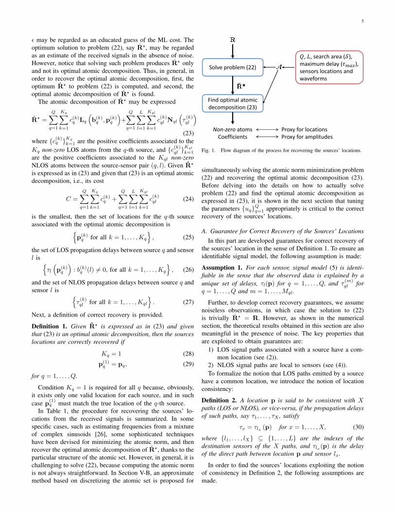
In Table 1, the procedure for recovering the sources’ lo-cations from the received signals is summarized. In somespecific cases, such as estimating frequencies from a mixtureof complex sinusoids [26], some sophisticated techniqueshave been devised for minimizing the atomic norm, and thenrecover the optimal atomic decomposition of R?, thanks to theparticular structure of the atomic set. However, in general, it ischallenging to solve (22), because computing the atomic normis not always straightforward. In Section V-B, an approximatemethod based on discretizing the atomic set is proposed for

Solve problem (22)

Find optimal atomic decomposition (23)

Non-zero atoms Coefficients

Proxy for locations Proxy for amplitudes

𝑄, 𝐿, search area (𝒮), maximum delay (𝜏𝑚𝑎𝑥), sensors locations, waveforms

𝑄, 𝐿, search area (𝒮), maximum delay (𝜏𝑚𝑎𝑥), sensors locations and waveforms

Fig. 1. Flow diagram of the process for recovering the sources’ locations.

simultaneously solving the atomic norm minimization problem(22) and recovering the optimal atomic decomposition (23).Before delving into the details on how to actually solveproblem (22) and find the optimal atomic decomposition asexpressed in (23), it is shown in the next section that tuningthe parameters {uq}Qq=1 appropriately is critical to the correctrecovery of the sources’ locations.

A. Guarantee for Correct Recovery of the Sources’ LocationsIn this part are developed guarantees for correct recovery of

the sources’ location in the sense of Definition 1. To ensure anidentifiable signal model, the following assumption is made:

Assumption 1. For each sensor, signal model (5) is identi-fiable in the sense that the observed data is explained by aunique set of delays, τl(p) for q = 1, . . . , Q, and τ

(m)ql for

q = 1, . . . , Q and m = 1, . . . ,Mql.

Further, to develop correct recovery guarantees, we assumenoiseless observations, in which case the solution to (22)is trivially R? = R. However, as shown in the numericalsection, the theoretical results obtained in this section are alsomeaningful in the presence of noise. The key properties thatare exploited to obtain guarantees are:

1) LOS signal paths associated with a source have a com-mon location (see (2)).

2) NLOS signal paths are local to sensors (see (4)).To formalize the notion that LOS paths emitted by a source

have a common location, we introduce the notion of locationconsistency:

Definition 2. A location p is said to be consistent with Xpaths (LOS or NLOS), or vice-versa, if the propagation delaysof such paths, say τ1, . . . , τX , satisfy

τx = τlx (p) for x = 1, . . . , X, (30)

where {l1, . . . , lX} ⊆ {1, . . . , L} are the indexes of thedestination sensors of the X paths, and τlx(p) is the delayof the direct path between location p and sensor lx.

In order to find the sources’ locations exploiting the notionof consistency in Definition 2, the following assumptions aremade.

6

Assumption 2. The number of LOS paths from source q, Sq ,is known.

By its very nature, a source location cannot be consistentwith any NLOS. Thus the location of the q-th source isconsistent with exactly Sq paths.

Assumption 3. Only the true location of the q-th source isconsistent with Sq paths emitted by the q-th source.

By Assumptions 2 and 3, given a source with a knownemitted waveform and a known number S of LOS paths, itstrue location is the only one consistent with S paths.

From (23) and Definition 1, the solution containing thetrue locations of the sources is associated with the optimalatomic decomposition. However, from (18) and the definitionof atoms, namely, LOS atoms (15) and NLOS atoms (16), theoptimal atomic decomposition is parameterized by the normof the amplitudes in the LOS atoms uq (15). For given dataR?, decreasing uq has to be balanced by an increase in thecoefficients of the LOS atoms, thus raising their contributionto the cost C (24). Put another way, different values of uq leadto different explanations of the data R? manifested as differentoptimal atomic decompositions, and thus corresponding todifferent solutions of the source localization problem. Weseek to determine which values of parameters uq ensure thatthe corresponding optimal atomic decomposition results inlocations that are consistent with the number of paths indicatedby Assumption 2. This in turn guarantees that these are the truesources’ locations. The next lemma establishes the conditionon uq under which a location associated with the optimalatomic decomposition is also consistent with the number ofLOS paths.

Lemma 1. Given a known number of LOS paths Sq of theq-th source, if parameter uq satisfies

uq <1√Sq − 1

, (31)

then any location (for the q-th source) associated to theoptimal atomic decomposition (25) is consistent, in the senseof Definition 2, with Sq or more paths.

For the proof of Lemma 1, see Appendix A. The interpre-tation of this lemma is that given a solution that producesa location with less than Sq paths, and if condition (31) ismet, there exists another lower cost solution, implying that asolution with fewer than Sq paths cannot be optimal.

The previous lemma guarantees that any location associatedwith the optimal atomic decomposition is consistent with Sqpaths. The next lemma establishes the condition on uq thatensures that at least one location is associated with the optimalatomic decomposition.

Lemma 2. Given a known number of LOS paths Sq of theq-th source, if parameter uq satisfies

uq >1√Sq, (32)

then at least one location (for the q-th source) is associatedto the optimal atomic decomposition.

For the proof of Lemma 2, see Appendix B. The interpre-tation of this lemma is that given a solution that does notproduce a location for the q-th source, and if condition (32)is met, there exists another lower cost solution that producesa location for the q-th source.

The two lemmas lead directly to the following theoremestablishing the guarantee for correct recovery of the sources’locations.

Theorem 1. A sufficient condition for the correct recovery inthe sense of Definition 1 of the sources’ locations is that

1√Sq

< uq <1√Sq − 1

(33)

for all q.

Proof: If uq > 1/√Sq for all q, by Lemma 2, at least one

location is associated to the optimal atomic decomposition foreach source. By Assumption 2, the number of LOS paths Sqis known for each source q. Therefore, if uq is chosen suchthat uq < 1/

√Sq−1 for all q, then by Lemma 1, the locations

associated to the optimal atomic decomposition for the sourceq are consistent with Sq or more paths. However, accordingto Assumption 3, only the location of the source is consistentwith Sq or more paths, thus completing the proof.

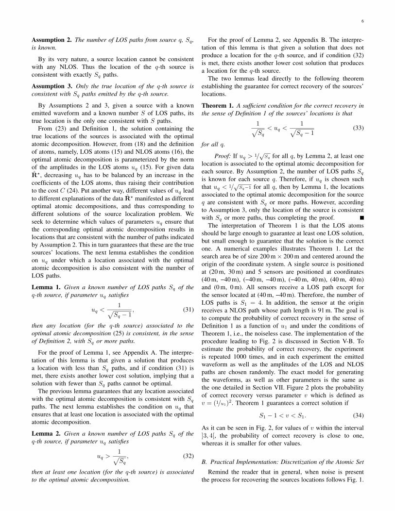
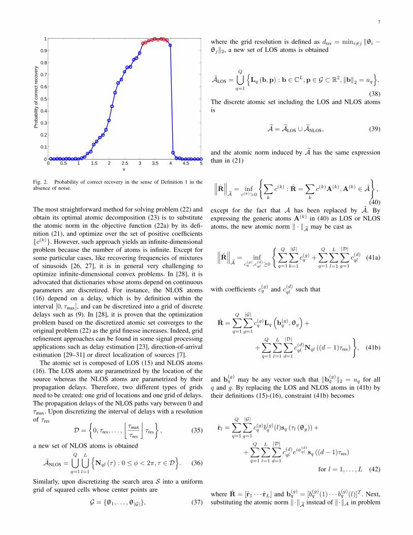
The interpretation of Theorem 1 is that the LOS atomsshould be large enough to guarantee at least one LOS solution,but small enough to guarantee that the solution is the correctone. A numerical examples illustrates Theorem 1. Let thesearch area be of size 200 m× 200 m and centered around theorigin of the coordinate system. A single source is positionedat (20 m, 30 m) and 5 sensors are positioned at coordinates(40 m, −40 m), (−40 m, −40 m), (−40 m, 40 m), (40 m, 40 m)and (0 m, 0 m). All sensors receive a LOS path except forthe sensor located at (40 m, −40 m). Therefore, the number ofLOS paths is S1 = 4. In addition, the sensor at the originreceives a NLOS path whose path length is 91 m. The goal isto compute the probability of correct recovery in the sense ofDefinition 1 as a function of u1 and under the conditions ofTheorem 1, i.e., the noiseless case. The implementation of theprocedure leading to Fig. 2 is discussed in Section V-B. Toestimate the probability of correct recovery, the experimentis repeated 1000 times, and in each experiment the emittedwaveform as well as the amplitudes of the LOS and NLOSpaths are chosen randomly. The exact model for generatingthe waveforms, as well as other parameters is the same asthe one detailed in Section VII. Figure 2 plots the probabilityof correct recovery versus parameter v which is defined asv = (1/u1)2. Theorem 1 guarantees a correct solution if

S1 − 1 < v < S1. (34)

As it can be seen in Fig. 2, for values of v within the interval]3, 4[, the probability of correct recovery is close to one,whereas it is smaller for other values.

B. Practical Implementation: Discretization of the Atomic Set

Remind the reader that in general, when noise is presentthe process for recovering the sources locations follows Fig. 1.

7

0 0.5 1 1.5 2 2.5 3 3.5 4 4.5 5 0

0.1

0.2

0.3

0.4

0.5

0.6

0.7

0.8

0.9

1

v

Pro

bab

ility

of

corr

ect

recovery

Fig. 2. Probability of correct recovery in the sense of Definition 1 in theabsence of noise.

The most straightforward method for solving problem (22) andobtain its optimal atomic decomposition (23) is to substitutethe atomic norm in the objective function (22a) by its defi-nition (21), and optimize over the set of positive coefficients{c(k)}. However, such approach yields an infinite-dimensionalproblem because the number of atoms is infinite. Except forsome particular cases, like recovering frequencies of mixturesof sinusoids [26, 27], it is in general very challenging tooptimize infinite-dimensional convex problems. In [28], it isadvocated that dictionaries whose atoms depend on continuousparameters are discretized. For instance, the NLOS atoms(16) depend on a delay, which is by definition within theinterval [0, τmax], and can be discretized into a grid of discretedelays such as (9). In [28], it is proven that the optimizationproblem based on the discretized atomic set converges to theoriginal problem (22) as the grid finesse increases. Indeed, gridrefinement approaches can be found in some signal processingapplications such as delay estimation [23], direction-of-arrivalestimation [29–31] or direct localization of sources [7].

The atomic set is composed of LOS (15) and NLOS atoms(16). The LOS atoms are parametrized by the location of thesource whereas the NLOS atoms are parametrized by theirpropagation delays. Therefore, two different types of gridsneed to be created: one grid of locations and one grid of delays.The propagation delays of the NLOS paths vary between 0 andτmax. Upon discretizing the interval of delays with a resolutionof τres

D =

{0, τres, . . . ,

⌊τmax

τres

⌋τres

}, (35)

a new set of NLOS atoms is obtained

ANLOS =

Q⋃q=1

L⋃l=1

{Nql (τ) : 0 ≤ φ < 2π, τ ∈ D

}. (36)

Similarly, upon discretizing the search area S into a uniformgrid of squared cells whose center points are

G = {θ1, . . . ,θ|G|}, (37)

where the grid resolution is defined as dres = mini 6=j ‖θi −θj‖2, a new set of LOS atoms is obtained

ALOS =

Q⋃q=1

{Lq (b,p) : b ∈ CL,p ∈ G ⊂ R2, ‖b‖2 = uq

}.

(38)The discrete atomic set including the LOS and NLOS atomsis

A = ALOS ∪ ANLOS, (39)

and the atomic norm induced by A has the same expressionthan in (21)

∥∥∥R∥∥∥A

= infc(k)>0

{∑k

c(k) : R =∑k

c(k)A(k),A(k) ∈ A

},

(40)except for the fact that A has been replaced by A. Byexpressing the generic atoms A(k) in (40) as LOS or NLOSatoms, the new atomic norm ‖ · ‖A may be cast as

∥∥∥R∥∥∥A

= infc(g)q ,c

(d)ql ≥0

{Q∑q=1

|G|∑k=1

c(g)q +

Q∑q=1

L∑l=1

|D|∑g=1

c(d)ql (41a)

with coefficients c(g)g and c(d)ql such that

R =

Q∑q=1

|G|∑g=1

c(g)q Lq

(b(g)q ,θg

)+

+

Q∑q=1

L∑l=1

|D|∑d=1

c(d)ql Nql ((d− 1)τres)

}, (41b)

and b(g)q may be any vector such that ‖b(g)

q ‖2 = uq for allq and g. By replacing the LOS and NLOS atoms in (41b) bytheir definitions (15)-(16), constraint (41b) becomes

rl =

Q∑q=1

|G|∑g=1

c(g)q b(g)q (l)sq (τl (θg)) +

+

Q∑q=1

L∑l=1

|D|∑d=1

c(d)ql e

iφ(d)ql sq ((d− 1)τres)

for l = 1, . . . , L (42)

where R = [r1 · · · rL] and b(g)q = [b

(g)q (1) · · · b(g)q (l)]T . Next,

substituting the atomic norm ‖·‖A instead of ‖·‖A in problem

8

(22) with (41a) and (42) yields

minc(g)q ,c

(d)ql ≥0

‖b(g)q ‖2=uq

0≤φ(d)ql <2π

Q∑q=1

|G|∑k=1

c(g)q +

Q∑q=1

L∑l=1

|D|∑g=1

c(d)ql (43a)

s.t.L∑l=1

‖rl − rl‖22 ≤ ε (43b)

rl =

Q∑q=1

|G|∑g=1

c(g)q b(g)q (l)sq (τl (θg)) +

+

Q∑q=1

L∑l=1

|D|∑d=1

c(d)ql e

iφ(d)ql sq ((d− 1)τres)

for l = 1, . . . , L.

(43c)

Problem (43) is not convex because of the bilinear forms,c(g)q b

(g)q (l) and c

(d)ql e

iφ(d)ql , appearing in constraint (43c). This

can be easily remedied by the following variable changes

c(g)q b(g)q = y(g)

q (44a)

c(d)ql e

iφ(d)ql = z(d)q (l), (44b)

from which it follows that∥∥∥c(g)q b(g)q

∥∥∥2

= c(g)q uq =∥∥∥y(g)

q

∥∥∥2

(45a)∣∣∣c(d)ql eiφ(d)ql

∣∣∣ = c(d)ql =

∣∣∣z(d)q (l)∣∣∣ . (45b)

Combining (44) and (45) with (43c) and (43a), respectively,results in the following optimization problem

miny(g)q

z(d)q (l)

Q∑q=1

|G|∑g=1

∥∥∥y(g)q

∥∥∥2

uq+

Q∑q=1

L∑l=1

|D|∑d=1

∣∣∣z(d)q (l)∣∣∣ (46a)

s.t.L∑l=1

‖rl − rl‖22 ≤ ε (46b)

rl =

Q∑q=1

|G|∑g=1

y(g)q (l)sq (τl(θg)) +

+

Q∑q=1

|D|∑d=1

z(d)q (l)sq ((d− 1)τres)

for l = 1, . . . , L,

(46c)

which is convex and finite-dimensional. Problem (46) is equiv-alent to the latent group Lasso problem [32], and specificalgorithms for solving (46) exist in the literature [33]. More-over, the problem also falls into the class of second-ordercone programs (SOCP), a subfamily of convex problems, forwhich efficient algorithms are available [34]. In our case, theSOCP type of algorithms resulted in the fastest computationaltimes. The variable y(g)q (l) represents the amplitude of a LOSpaths from source q to sensor l with delay τl(θg), whereasthe variable z(d)q (l) represents the amplitude of a NLOS pathfrom source q to sensor l with delay (d−1)τres. Let {y(g)

q } and{z(g)q (l)} be the solutions to problem (46). Then, the location

of the q-th source is the grid location θg for which ‖y(g)q ‖2

is larger than zero. Intuitively speaking, minimizing the term∑Qq=1

∑Ll=1

∑|D|d=1 |z

(d)q (l)| in the objective function (46a)

induces a sparse number of NLOS paths, whereas minimizing∑Qq=1

∑|G|g=1 ‖y

(g)q ‖2 induces a sparse number of sources’

locations.

C. Estimation of the Number of LOS Sensors

According to Theorem 1, we must fix uq to a value thatsatisfies 1/

√Sq < uq < 1/

√Sq−1 for each source q, where Sq

is the number of sensors receiving a LOS component fromthe q-th source. Hence, uq must be set to uq = 1/

√Sq−µ for a

parameter µ ∈]0, 1[. For instance, it has been observed that asatisfactory choice is µ = 0.2 as it led to the best probabilityof correct recovery for all experiments in Section VII. Inthis section, we propose a method for estimating the sourceslocations that not only does not require a priori knowledge onthe number of LOS sensors Sq , but in fact estimates them.The method works as follows. We start by assuming that allsensors receive a LOS component from all sources, Sq = Lfor all q, and set uq such that it satisfies (33). Then problem(46) is solved. According to Lemma 1, the sources’ locationsassociated to the optimal atomic decomposition for the q-thsource are consistent with at least Sq paths. However, byAssumption 3, no location is consistent with more than Sqpaths. Therefore, if the number of LOS sensors (Sq > Sq) hadbeen overestimated, no location would be obtained for sourceq. In the next step, Sq is decreased by one for all those sourceswithout a location estimate, and problem (46b) is solved again.These steps are repeated until a location is obtained for eachsource. The last value of Sq is the estimated number LOSsensors for the q-th source. This method corresponds to steps10, 11, 20–28 of DLM’s algorithm described in Section VI.

D. Spurious Locations

It is observed in numerical simulations that when thesources are off-grid (pq /∈ G for any q) and/or when thepropagation delays of the paths are off-grid (τ (m)

ql , τl(pq) /∈ Dfor any q, l, m), then some spurious locations may be obtainedfrom problem (46). This phenomenon is not new and it wasstudied in [35] in the case of delay estimation using the `1-norm (11). It was shown that if the propagation delay of a pathis off-grid, a peak appears around such propagation delay butalso secondary peaks of much weaker strength appear furtherapart.

To eliminate spurious locations, it is set a simple thresholdcriterion. Let y(g)

q be, for all q and g, the solution to problem(46). Ideally, for each source q, ‖y(g)

q ‖ is zero for all g exceptif θg matches the location of the source. However, in practice,for a given source q, problem (46) may produce some spuriouslocations, in which case ‖y(g)

q ‖ may be different than zerofor more than a single value of g. If θg is the true locationof the q-th source, then the Sq largest components of y

(g)q

are the amplitudes of the Sq LOS paths. In contrast, if θgis a spurious location, we have observed through numericalexperimentation that some of the Sq largest entries will be

9

approximately zero. Denote y(g)↓q the vector with the same

components than y(g)q , but sorted in descending order, i.e.,

|y(g)↓q (1)| ≥ · · · ≥ |y(g)↓q (L)|. We propose that, for a givensource q, all locations whose Sq strongest components do nosatisfy ∣∣∣y(g)↓q

(Sq

)∣∣∣ > AT. (47)

are dismissed. Here, Sq is the number of LOS paths assumedfor source q as explained in more detail in Section V-C,parameter A is the largest signal strength of a LOS or NLOSpath

A = max

(maxg,q,l

∣∣∣y(g)q (l)∣∣∣ ,max

d,q,l

∣∣∣z(d)q (l)∣∣∣) , (48)

and T is a value smaller than 1. For instance, in the simulationsit was used T = 1/30, so that all locations whose signalstrengths are 20 log10(30) ≈ 30 dB weaker than the strongestpath are discarded. If after the threshold criterion (47) oneor more locations still remain for the q-th source, then thelocation with the largest strength is picked

pq = θg : g = arg maxg

∣∣∣y(g)↓q

(Sq

)∣∣∣ . (49)

It is important to not skip (47), and apply (49) directly.As explained in Section V-C, the proposed technique worksby initially assuming that the number of LOS paths forthe q-th source is Sq = L and if no location is obtained,then successively decreasing Sq until problem (46) outputs alocation. However, if the threshold criterion (47) is skippedand Sq > Sq , a spurious location may be erroneously selectedas the correct source location instead of concluding that thereis no location and that Sq needs to be decreased.

E. Tuning Parameter εParameter ε in optimization problem (46) constraints the

fitting error between the received signals and the estimatedsignals. Such a parameter is set so that the received signalswithout noise are a feasible solution. Let rl be the noiselessreceived signal at sensor l, then we require that

L∑l=1

‖rl − rl‖22 =

L∑l=1

‖wl‖22 ≤ ε. (50)

If ε is chosen too small, then it can happen that∑Ll=1 ‖wl‖22 ≮

ε, thus excluding the noiseless signals from the set of possiblesolutions. Because the noise {wl}Ll=1 are random independentcomplex Gaussian vectors of length N , it follows that theerror normalized by the noise variance 2σ−2w

∑Ll=1 ‖wl‖22 is

a Chi-square random variable with 2NL degrees of freedom.Thus, parameter ε must be set to a large enough value so that∑Ll=1 ‖wl‖22 ≤ ε is satisfied with high probability, e.g.,

Pr

(L∑l=1

‖wl‖22 ≤ ε

)= γ. (51)

Let F(x, k) be the cumulative distribution function of the chi-squared distribution with k degrees of freedom evaluated at xand F−1 its inverse function. Then

ε =σ2w

2F−1 (γ, 2NL) . (52)

At low signal-to-noise ratio (SNR), it is possible that theenergy of the received signals is too low compared to theenergy of the noise causing that

∑Ll=1 ‖rl‖22 ≤ ε. In such case

problem (46) has the trivial solution y(g)q (l) = z

(g)q (l) = 0

for all q, l, g and d, and it will not output any locations.If∑Ll=1 ‖rl‖22 ≤ ε, we propose to estimate the locations by

finding the LOS signals that have the highest correlation withthe received signals:

pq = arg maxp∈G

L∑l=1

∣∣sHq (τl (p)) rl∣∣2∥∥sHq (τl (p))∥∥2 . (53)

F. Grid Refinement

The computational complexity of minimizing the second-order cone problem (46) is O((Q|G| + QL|D|)3.5) [36]. Tolower it we propose a recursive grid refinement procedureinspired by the ones in [29–31]. The optimization problem(46) employs a grid of delays in order to estimate the NLOSpaths between every source-sensor pair, and a grid of locationsin order to estimate the location of every source. In total,there are Q grids of location and QL grids of delays. Incomparison to previous grid refinement approaches, ours isa more complex due to the two different types of grids usedto explain the observed data. The idea behind a grid refinementprocedure is to start with a coarse grid(s) and refine eachgrid only around the active points. Let τres and dres be thegrid resolutions we wish to achieve in the grids of delays andlocations, respectively, and suppose that in order to lower thecomputational complexity, the grids are refined R times. If theresolution of the grids is increased by a factor of two at everystep, then the grids resolutions at each step are

τres,r = 2R−rτres for r = 1, . . . , R (54)

dres,r = 2R−rdres for r = 1, . . . , R. (55)

Let Dql,r be the grid of delays for the source-sensor pair (q, l)at step r, and Gq,r the grid of locations for source q. At thefirst step (r = 1), the continuous set of delays [0, τmax] isdiscretized with resolution τres,1

Dql,1 = {i τres,1 ∈ [0, τmax] : i ∈ Z} , (56a)

and the search area S is discretized uniformly with resolutiondres,1

Gq,1 =

{dres,1

(ij

)∈ S : i, j ∈ Z

}, (56b)

where Z is the set of integers. Consider step r, and let theactive propagation delays between the source-sensor pair (q, l)

be {τ (m)ql,r : m = 1, . . . , Mql,r}, and the active locations for

source q be {p(m)q,r : m = 1, . . . , Kq,r}. Then, the grids at step

r + 1 include the previous active delays and locations plussome neighbor points. For instance, in addition to the activedelays and locations, we include two points at the left andright of the active delays

Dql,r+1 =

Mql,r⋃m=1

{τ(m)ql,r + i τres,r+1 : i = −2,−1, 0, 1, 2

},

(57a)

10

𝜏∗ 𝜏∗ + 𝜏res(2)

𝜏∗ + 𝜏res(2)

− 𝜏res(3)

Step 1

θ∗ θ∗ +𝑑res(2)

−𝑑res(2)

θ∗ +𝑑res(2)

−𝑑res(2)

+ −𝑑res(3)

0

Step 2 Step 3

Estimate:

Estimate:

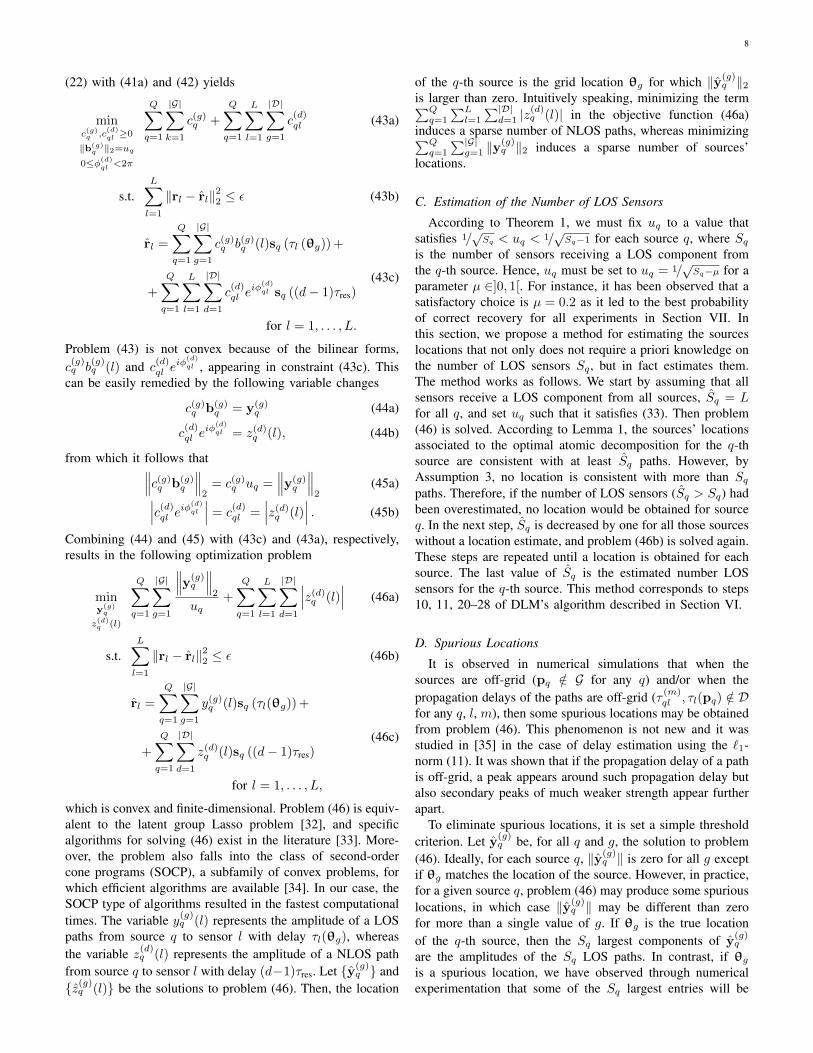
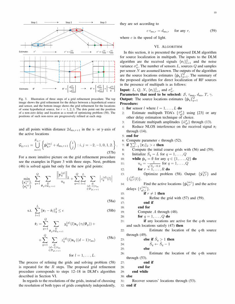
Fig. 3. Illustration of three steps of a grid refinement procedure. The topimage shows the grid refinement for the delays between a hypothetical sourceand sensor, and the bottom image shows the grid refinement for the locationsof some hypothetical source, for r = 1, 2, 3. The dots point out the positionof a non-zero delay and location as a result of optimizing problem (58). Thepositions of such non-zeros are progressively refined at each step.

and all points within distance 2dres,r+1 in the x- or y-axis ofthe active locations

Gq,r+1 =

Kq,r⋃m=1

{p(m)q,r + dres,r+1

(ij

): i, j = −2,−1, 0, 1, 2.

}.

(57b)For a more intuitive picture on the grid refinement proceduresee the examples in Figure 3 with three steps. Next, problem(46) is solved again but only for the new grid points:

min{y(g)

q },{z(d)

q }

Q∑q=1

∑g:

θg∈Gq,r+1

∥∥∥y(g)q

∥∥∥2

uq+

Q∑q=1

L∑l=1

∑d:

(d−1)τres∈Dql,r+1

∣∣∣z(d)q (l)∣∣∣

(58a)

s.t.L∑l=1

‖rl − rl‖22 ≤ ε (58b)

rl =

Q∑q=1

∑g:

θg∈Gq,r+1

y(g)q (l)sq (τl(θg)) +

+

Q∑q=1

∑d:

(d−1)τres∈Dql,r+1

z(d)q (l)sq ((d− 1)τres)

for l = 1, . . . , L.

(58c)

The process of refining the grids and solving problem (58)is repeated for the R steps. The proposed grid refinementprocedure corresponds to steps 12–18 in DLM’s algorithmdescribed in Section VI.

In regards to the resolutions of the grids, instead of choosingthe resolution of both types of grids completely independently,

they are set according to

c τres,r = dres,r for any r, (59)

where c is the speed of light.

VI. ALGORITHM

In this section, it is presented the proposed DLM algorithmfor source localization in multipath. The inputs to the DLMalgorithm are the received signals {rl}Ll=1 and the noisevariance σ2

w. The number of sensors L, sources Q and samplesper sensor N are assumed known. The outputs of the algorithmare the source locations estimates {pq}Qq=1. The summary ofthe proposed algorithm for direct localization of RF sourcesin the presence of multipath is as follows:Input: L, Q, N , {rl}Ll=1 and σ2

w.Parameters that need to be selected: S, τmax, dres, T , γ.Output: The source locations estimates {pq}Qq=1

Procedure:1: for sensor l where l = 1, . . . , L do2: Estimate multipath TOA’s {τpql} using [23] or any

other delay estimation technique of choice.3: Estimate multipath amplitudes {αpql} through (13).4: Reduce NLOS interference on the received signal rl

through (14).5: end for6: Compute parameter ε through (52).7: if

∑Ll−1 ‖rl‖2 > ε then

8: Compute the initial coarse grids with (56) and (59).9: Initialize Sq = L for q = 1, . . . , Q

10: while pq = ∅ for any q ∈ {1, . . . , Q} do11: uq = 1√

Sq−0.2for q = 1, . . . , Q

12: for r = 1, . . . , R do13: Optimize problem (58). Output: {y(g)

q,r} and{z(d)q,r (l)}.

14: Find the active locations {p(m)q,r } and the active

delays {τ (m)ql,r }.

15: if r 6= 1 then16: Refine the grid with (57) and (59).17: end if18: end for19: Compute A through (48).20: for q = 1, . . . , Q do21: if any locations are active for the q-th source

and such locations satisfy (47) then22: Estimate the location of the q-th source

through (49).23: else if Sq > 1 then24: Sq ← Sq − 125: else26: Estimate the location of the q-th source

through (53).27: end if28: end for29: end while30: else31: Recover sources’ locations through (53).32: end if

11

-100 -50 0 50 100 -100

-80

-60

-40

-20

0

20

40

60

80

100

source

sensors

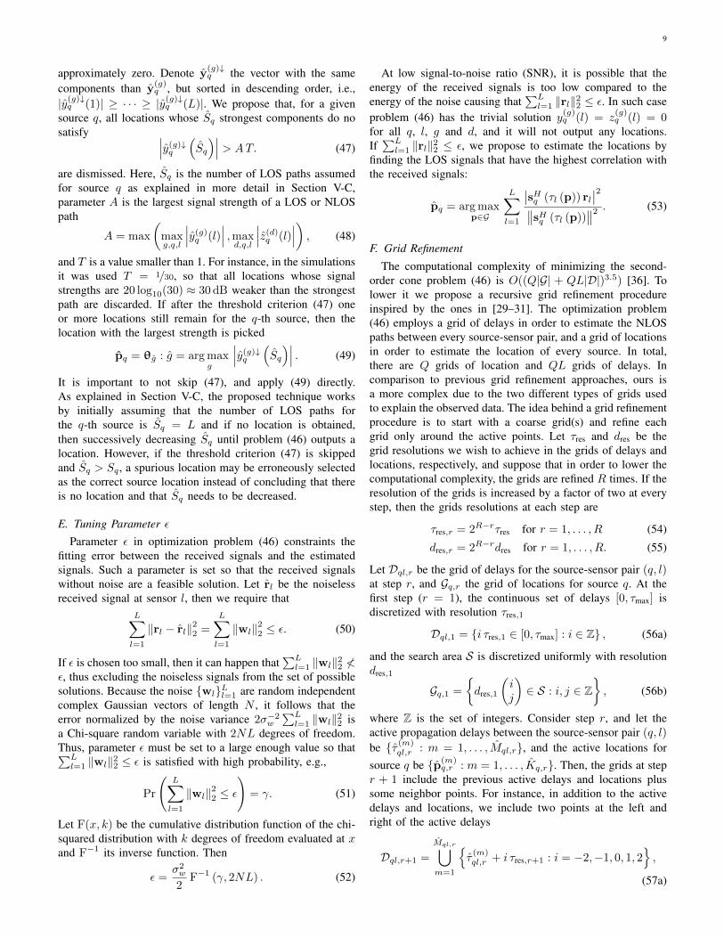
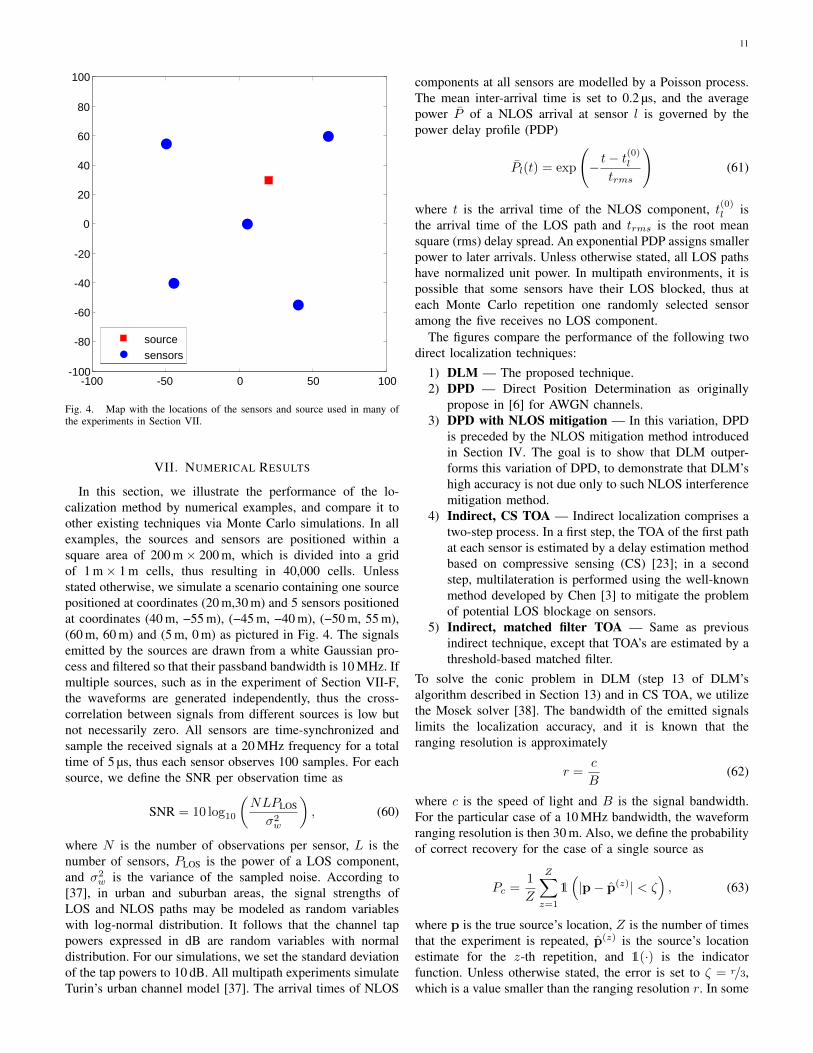
Fig. 4. Map with the locations of the sensors and source used in many ofthe experiments in Section VII.

VII. NUMERICAL RESULTS

In this section, we illustrate the performance of the lo-calization method by numerical examples, and compare it toother existing techniques via Monte Carlo simulations. In allexamples, the sources and sensors are positioned within asquare area of 200 m× 200 m, which is divided into a gridof 1 m× 1 m cells, thus resulting in 40,000 cells. Unlessstated otherwise, we simulate a scenario containing one sourcepositioned at coordinates (20 m,30 m) and 5 sensors positionedat coordinates (40 m, −55 m), (−45 m, −40 m), (−50 m, 55 m),(60 m, 60 m) and (5 m, 0 m) as pictured in Fig. 4. The signalsemitted by the sources are drawn from a white Gaussian pro-cess and filtered so that their passband bandwidth is 10 MHz. Ifmultiple sources, such as in the experiment of Section VII-F,the waveforms are generated independently, thus the cross-correlation between signals from different sources is low butnot necessarily zero. All sensors are time-synchronized andsample the received signals at a 20 MHz frequency for a totaltime of 5 µs, thus each sensor observes 100 samples. For eachsource, we define the SNR per observation time as

SNR = 10 log10

(NLPLOS

σ2w

), (60)

where N is the number of observations per sensor, L is thenumber of sensors, PLOS is the power of a LOS component,and σ2

w is the variance of the sampled noise. According to[37], in urban and suburban areas, the signal strengths ofLOS and NLOS paths may be modeled as random variableswith log-normal distribution. It follows that the channel tappowers expressed in dB are random variables with normaldistribution. For our simulations, we set the standard deviationof the tap powers to 10 dB. All multipath experiments simulateTurin’s urban channel model [37]. The arrival times of NLOS

components at all sensors are modelled by a Poisson process.The mean inter-arrival time is set to 0.2 µs, and the averagepower P of a NLOS arrival at sensor l is governed by thepower delay profile (PDP)

Pl(t) = exp

(−t− t(0)ltrms

)(61)

where t is the arrival time of the NLOS component, t(0)l isthe arrival time of the LOS path and trms is the root meansquare (rms) delay spread. An exponential PDP assigns smallerpower to later arrivals. Unless otherwise stated, all LOS pathshave normalized unit power. In multipath environments, it ispossible that some sensors have their LOS blocked, thus ateach Monte Carlo repetition one randomly selected sensoramong the five receives no LOS component.

The figures compare the performance of the following twodirect localization techniques:

1) DLM — The proposed technique.2) DPD — Direct Position Determination as originally

propose in [6] for AWGN channels.3) DPD with NLOS mitigation — In this variation, DPD

is preceded by the NLOS mitigation method introducedin Section IV. The goal is to show that DLM outper-forms this variation of DPD, to demonstrate that DLM’shigh accuracy is not due only to such NLOS interferencemitigation method.

4) Indirect, CS TOA — Indirect localization comprises atwo-step process. In a first step, the TOA of the first pathat each sensor is estimated by a delay estimation methodbased on compressive sensing (CS) [23]; in a secondstep, multilateration is performed using the well-knownmethod developed by Chen [3] to mitigate the problemof potential LOS blockage on sensors.

5) Indirect, matched filter TOA — Same as previousindirect technique, except that TOA’s are estimated by athreshold-based matched filter.

To solve the conic problem in DLM (step 13 of DLM’salgorithm described in Section 13) and in CS TOA, we utilizethe Mosek solver [38]. The bandwidth of the emitted signalslimits the localization accuracy, and it is known that theranging resolution is approximately

r =c

B(62)

where c is the speed of light and B is the signal bandwidth.For the particular case of a 10 MHz bandwidth, the waveformranging resolution is then 30 m. Also, we define the probabilityof correct recovery for the case of a single source as

Pc =1

Z

Z∑z=1

1(|p− p(z)| < ζ

), (63)

where p is the true source’s location, Z is the number of timesthat the experiment is repeated, p(z) is the source’s locationestimate for the z-th repetition, and 1(·) is the indicatorfunction. Unless otherwise stated, the error is set to ζ = r/3,which is a value smaller than the ranging resolution r. In some

12

0 5 10 15 20 25 300

0.5

1

1.5

2

2.5

3

3.5

SNR [dB]

No

rma

lize

d r

MS

E

DLM

DPD / DPD with NLOS mitigation

indirect, CS TOA

indirect, matched filter TOA

Fig. 5. Root mean square error vs. SNR for the scenario in Fig. 4 when nomultipath is present.

0 5 10 15 20 25 300

0.1

0.2

0.3

0.4

0.5

0.6

0.7

0.8

0.9

1

SNR [dB]

Pro

ba

bili

ty o

f co

rre

ct

reco

ve

ry

DLM

DPD / DPD with NLOS mitigation

indirect, CS TOA

indirect, matched filter TOA

Fig. 6. Probability of correct recovery vs. SNR for the scenario in Fig. 4when no multipath is present.

of the tests, it is plotted the normalized root mean square error

rMSE =1

r

√√√√ 1

Z

Z∑z=1

(p− p(z)

)2. (64)

All experiments are repeated 1000 times, i.e., Z = 1000.

A. Performance in the Absence of Multipath

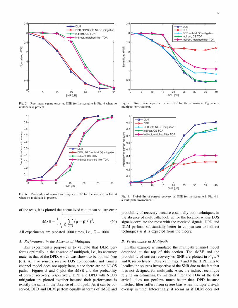
This experiment’s purpose is to validate that DLM per-forms optimally in the absence of multipath, i.e., its accuracymatches that of the DPD, which was shown to be optimal (see[6]). All five sensors receive LOS components, and Turin’schannel model does not apply here, since there are no NLOSpaths. Figures 5 and 6 plot the rMSE and the probabilityof correct recovery, respectively. DPD and DPD with NLOSmitigation are plotted together because their performance isexactly the same in the absence of multipath. As it can be ob-served, DPD and DLM perfom equally in terms of rMSE and

0 5 10 15 20 25 30 35 400

0.5

1

1.5

2

2.5

3

3.5

SNR [dB]

No

rma

lize

d r

MS

E

DLM

DPD

DPD with NLOS mitigation

indirect, CS TOA

indirect, matched filter TOA

Fig. 7. Root mean square error vs. SNR for the scenario in Fig. 4 in amultipath environment.

0 5 10 15 20 25 30 35 400

0.1

0.2

0.3

0.4

0.5

0.6

0.7

0.8

0.9

1

SNR [dB]

Pro

ba

bili

ty o

f co

rre

ct

reco

ve

ry

DLM

DPD

DPD with NLOS mitigation

indirect, CS TOA

indirect, matched filter TOA

Fig. 8. Probability of correct recovery vs. SNR for the scenario in Fig. 4 ina multipath environment.

probability of recovery because essentially both techniques, inthe absence of multipath, look up for the location whose LOSsignals correlate the most with the received signals. DPD andDLM perform substantially better in comparison to indirecttechniques as it is expected from the theory.

B. Performance in Multipath

In this example is simulated the multipath channel modeldescribed at the top of this section. The rMSE and theprobability of correct recovery vs. SNR are plotted in Figs. 7and 8, respectively. Observe in Figs. 7 and 8 that DPD fails tolocalize the sources irrespective of the SNR due to the fact thatit is not designed for multipath. Also, the indirect techniquerelying on estimating by matched filter the TOA of the firstarrival, does not perform much better than DPD becausematched filter suffers from severe bias when multiple arrivalsoverlap in time. Interestingly, it seems as if DLM does not

13

0.2 0.4 0.6 0.8 1 1.2 1.4 1.6 1.8 20

0.1

0.2

0.3

0.4

0.5

0.6

0.7

0.8

0.9

1

Normalized error

Pro

babili

ty o

f corr

ect re

covery

DLM

DPD

DPD with NLOS mitigation

indirect, CS TOA

indirect, matched filter TOA

Fig. 9. Probability of correct recovery vs. error for the scenario in Fig. 4for a 30 dB SNR.

perform better, in terms of rMSE, than the indirect techniqueemploying CS TOA estimates. In Fig. 9, the probability ofcorrect recovery (63) is plotted for different errors rangingfrom 0 to 2r for an SNR value of 30 dB. DLM achieves ahigh probability of correct recovery for much smaller errorsthan the other methods. For instance, DLM’s probability ofcorrect recovery is 0.9 for an error smaller than 0.4r, whereasfor the indirect technique with CS TOA, such probability isonly achieved when the error is 0.9r. The other techniquesperform substantially worse than DLM, and in fact, they neverachieve a probability of recovery close to one even when verylarge errors are allowed. In summary, DLM can achieve ahigh probability of recovery for very small errors. In terms ofrMSE, DLM and the indirect technique employing CS TOAestimates perform similarly, because in the rMSE metric smallerrors have a much smaller impact compared to the largeerrors. Hence, in the next experiments, we focus only on theprobability of correct recovery.

C. Probability of Correct Recovery vs. Delay Spread

The considered channel model depends on the rms delayspread, which determines the interval between the LOS com-ponent and the last arriving NLOS component. In general,larger delay spreads imply more multipath that make thelocalization more challenging. In Fig. 10, the probability ofcorrect recovery is plotted for an rms delay spread rangingfrom 0 to 0.6 µs at 30 dB SNR. At high-SNR and at a zerodelay spread all localization techniques perform similarly.However, as soon as the rms delay spread increases bya little as 0.2 µs, DPD’s performance drops markedly. Thetechniques specifically designed for multipath channels, suchas the indirect technique based on CS TOA estimates andDLM, degrade very slightly as the rms delay spread increases.DLM outperforms all other techniques and is capable ofrecovering the sources locations with a high probability ofcorrect recovery irrespective of the delay spread.

0 0.1 0.2 0.3 0.4 0.50.2

0.3

0.4

0.5

0.6

0.7

0.8

0.9

1

RMS delay [us]

Pro

ba

bili

ty o

f co

rre

ct

reco

ve

ry

DLM

DPD

DPD with NLOS mitigation

indirect, CS TOA

indirect, matched filter TOA

Fig. 10. Probability of correct recovery vs. rms delay spread for the scenarioin Fig. 4 in a multipath environment for a 30 dB SNR.

1 2 3 4 5 6 70

0.2

0.4

0.6

0.8

1

Number of grid refinement steps

Pro

ba

bili

ty o

f co

rre

ct

reco

ve

ry

1 2 3 4 5 6 70

5

10

15

20

25

30

Ave

rag

e e

lap

se

d t

ime

[s]

Fig. 11. The left axis plots the probability of correct recovery and the rightaxis the mean elapsed time for running DLM’s Stage 2, vs. the number ofgrid refinement steps. The SNR is fixed at 30 dB.

D. Probability of Correct Recovery vs. Number of Grid Re-finement Steps

The purpose of the grid refinement procedure introducedin Section V-F is to reduce the computational complexity ofDLM, while maintaining the localization accuracy. Figure 11plots the probability of correct recovery (square marker) andthe DLM’s mean elapsed time at Stage 2 (circle marker),versus the number of grid refinement steps. The SNR is fixed at30 dB. DLM is run on a computer with an Intel Xeon processorat 2.8 GHz with 4 GB of RAM memory. Perhaps surprisingly,the probability of correct recovery remains almost constantirrespective of the number of steps. The lowest computationaltime is 5 s and is obtained for five grid refinement steps. Thenumber of grid steps that results in the lowest computationaltime depends on many factors such as number of grid points,efficiency of the conic solver, particular scenario and so forth.

14

0 5 10 15 20 25 30 35 400

0.1

0.2

0.3

0.4

0.5

0.6

0.7

0.8

0.9

1

SNR [dB]

Pro

babili

ty o

f corr

ect re

cove

ry

5 LOS sensors

4 LOS sensors

3 LOS sensors

2 LOS sensors

1 LOS sensor

Fig. 12. Probability of correct recovery vs. the number of LOS sensors fora 30 dB SNR.

Thus, in general, the optimum number of steps must be foundby in situ testing.

E. Number of LOS sensors

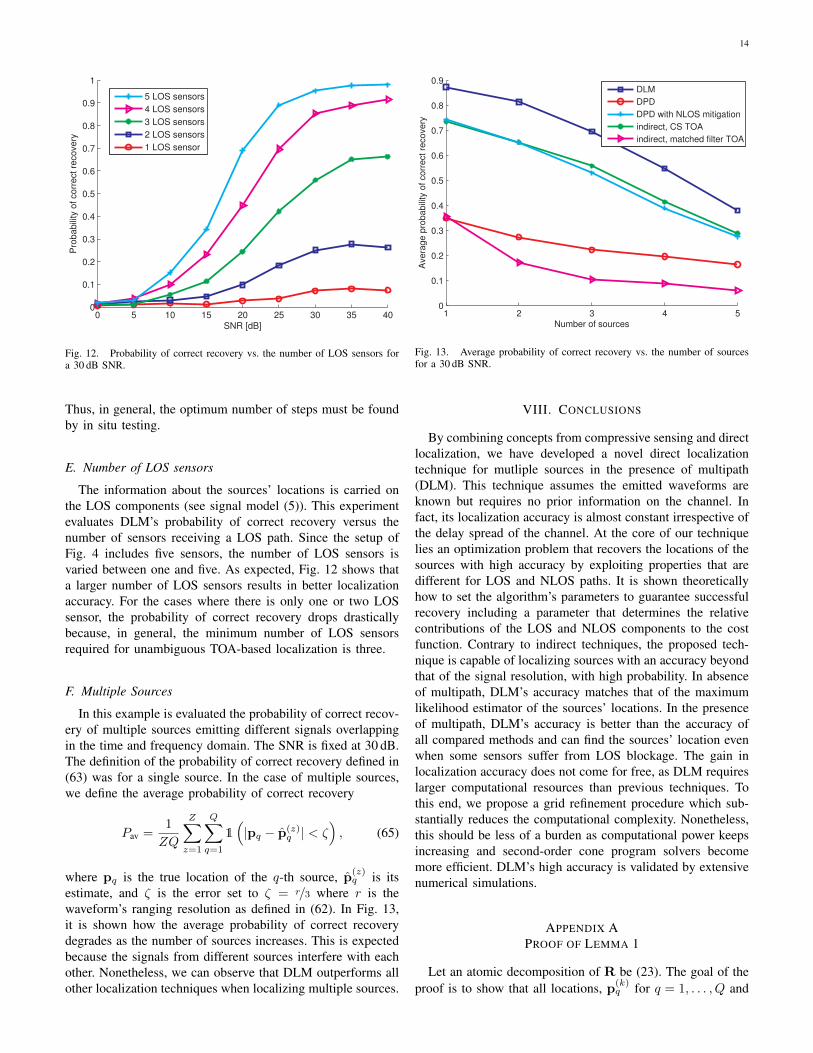
The information about the sources’ locations is carried onthe LOS components (see signal model (5)). This experimentevaluates DLM’s probability of correct recovery versus thenumber of sensors receiving a LOS path. Since the setup ofFig. 4 includes five sensors, the number of LOS sensors isvaried between one and five. As expected, Fig. 12 shows thata larger number of LOS sensors results in better localizationaccuracy. For the cases where there is only one or two LOSsensor, the probability of correct recovery drops drasticallybecause, in general, the minimum number of LOS sensorsrequired for unambiguous TOA-based localization is three.

F. Multiple Sources

In this example is evaluated the probability of correct recov-ery of multiple sources emitting different signals overlappingin the time and frequency domain. The SNR is fixed at 30 dB.The definition of the probability of correct recovery defined in(63) was for a single source. In the case of multiple sources,we define the average probability of correct recovery

Pav =1

ZQ

Z∑z=1

Q∑q=1

1(|pq − p(z)

q | < ζ), (65)

where pq is the true location of the q-th source, p(z)q is its

estimate, and ζ is the error set to ζ = r/3 where r is thewaveform’s ranging resolution as defined in (62). In Fig. 13,it is shown how the average probability of correct recoverydegrades as the number of sources increases. This is expectedbecause the signals from different sources interfere with eachother. Nonetheless, we can observe that DLM outperforms allother localization techniques when localizing multiple sources.

1 2 3 4 50

0.1

0.2

0.3

0.4

0.5

0.6

0.7

0.8

0.9

Number of sources

Ave

rag

e p

rob

ab

ility

of

co

rre

ct

reco

ve

ry

DLM

DPD

DPD with NLOS mitigation

indirect, CS TOA

indirect, matched filter TOA

Fig. 13. Average probability of correct recovery vs. the number of sourcesfor a 30 dB SNR.

VIII. CONCLUSIONS

By combining concepts from compressive sensing and directlocalization, we have developed a novel direct localizationtechnique for mutliple sources in the presence of multipath(DLM). This technique assumes the emitted waveforms areknown but requires no prior information on the channel. Infact, its localization accuracy is almost constant irrespective ofthe delay spread of the channel. At the core of our techniquelies an optimization problem that recovers the locations of thesources with high accuracy by exploiting properties that aredifferent for LOS and NLOS paths. It is shown theoreticallyhow to set the algorithm’s parameters to guarantee successfulrecovery including a parameter that determines the relativecontributions of the LOS and NLOS components to the costfunction. Contrary to indirect techniques, the proposed tech-nique is capable of localizing sources with an accuracy beyondthat of the signal resolution, with high probability. In absenceof multipath, DLM’s accuracy matches that of the maximumlikelihood estimator of the sources’ locations. In the presenceof multipath, DLM’s accuracy is better than the accuracy ofall compared methods and can find the sources’ location evenwhen some sensors suffer from LOS blockage. The gain inlocalization accuracy does not come for free, as DLM requireslarger computational resources than previous techniques. Tothis end, we propose a grid refinement procedure which sub-stantially reduces the computational complexity. Nonetheless,this should be less of a burden as computational power keepsincreasing and second-order cone program solvers becomemore efficient. DLM’s high accuracy is validated by extensivenumerical simulations.

APPENDIX APROOF OF LEMMA 1

Let an atomic decomposition of R be (23). The goal of theproof is to show that all locations, p(k)

q for q = 1, . . . , Q and

15

k = 1, . . . ,Kq are consistent with Sq or more paths if∥∥∥p(k)q

∥∥∥2

= uq <1√Sq − 1

. (66)

From (23), the signal at the l-th sensor is

rl =

Q∑q=1

Kq∑k=1

b(k)q (l) 6=0

c(k)q b(k)q (l)sq

(τl

(p(k)q

))+

+

Q∑q=1

Kql∑k=1

c(k)ql e

iφ(k)ql sq

(τ(k)ql

). (67)

By Assumption 3, τl(p(k)q ) is a true propagation if b(k)q (l) 6= 0.

Therefore, if b(k)q has Sq or more non-zero entries, according

to Definition 2, p(k)q is consistent with Sq or more paths. It is

left to prove that ‖b(k)q ‖0 ≥ Sq . The proof is by contradiction.

For instance, ∥∥∥b(1)1

∥∥∥0< S1. (68)

and let the atomic decomposition (23) in which the atomL1

(b(1)1 ,p

(1)1

)is replaced by ‖b(k)

q ‖0 NLOS atoms as fol-lows

L1

(b(1)1 ,p

(1)1

)=

L∑l=1

b(1)1 (l)6=0

∣∣∣b(1)1 (l)∣∣∣N11

(τl

(p(1)1

)). (69)

Consider now the two decompositions (23) and the oneobtained with (69). The costs of the two decompositions differonly in the coefficients of the atoms shown in (69). Ignoringthe common atoms, the cost of decomposition (23) is c(1)1 ,whereas the cost of decomposition obtained from combining(69) with (23) is

c(1)1

L∑l=1

b(1)1 (l)6=0

∣∣∣b(1)1 (l)∣∣∣ . (70)

Normalizing the two costs by c(1)1 , and if (23), which by (68)has a location p

(1)1 with less than Sq paths, is optimal, then

1 ≤L∑l=1

b(1)1 (l)6=0

∣∣∣b(1)1 (l)∣∣∣ . (71)

We show next that inequality (71) cannot be satisfied if‖b(1)

1 ‖2 satisfies (66). Define the vector function 1(b(1)1 )

whose l-th entry is one if b(1)1 (l) 6= 0, and 0 otherwise, anddenote | · | the element-wise absolute value. Then the righthand side of (71) is

L∑l=1

b(1)1 (l) 6=0

∣∣∣b(1)1 (l)∣∣∣ =

[1(b(1)1

)]T ∣∣∣b(1)1

∣∣∣ , (72)

and by the Cauchy-Schwarz inequality[1(b(1)1

)]T ∣∣∣b(1)1

∣∣∣ ≤≤∥∥∥1(b(1)

1

)∥∥∥2

∥∥∥b(1)1

∥∥∥2

=

√∥∥∥b(1)1

∥∥∥0

∥∥∥b(1)1

∥∥∥2. (73)

However, ‖b(1)1 ‖2 = u1, and by equation (66), ‖b(1)

1 ‖2 <1/√S1−1. Moreover, by assumption (68), ‖b(1)

1 ‖0 ≤ S1 − 1.Therefore, it follows√∥∥∥b(1)

1

∥∥∥0

∥∥∥b(1)1

∥∥∥2< 1, (74)

which combined with (72) and (73) results inL∑l=1

b(1)1 (l) 6=0

∣∣∣b(1)1 (l)∣∣∣ < 1, (75)

which contradicts (71).

APPENDIX BPROOF OF LEMMA 2

Let (23) be an atomic decomposition of R. Recall thatparameter Kq is the number of locations associated to theoptimal atomic decomposition for the q-th source. We aim toprove that if parameter uq∥∥∥b(k)

q

∥∥∥2

= uq >1√Sq, (76)

then the optimal decomposition has Kq ≥ 1. The proof is bycontradiction. Let K1 = 0, then a presumed optimal atomicdecomposition (23) simplifies to

R =

Q∑q=2

Kq∑k=1

c(k)q Lq

(b(k)q ,p(k)

q

)+

Q∑q=1

L∑l=1

Kql∑k=1

c(k)ql Nql

(τ(k)ql

).

(77)From (77), the signal at the l-th sensor is

rl =

Q∑q=2

Kq∑k=1

b(k)q (l)6=0

c(k)q b(k)q (l)sq

(τl

(p(k)q

))+

+

Q∑q=1

Kql∑k=1

c(k)ql e

iφ(k)ql sq

(τ(k)ql

). (78)

Notice that the first summation begins with q = 2, becauseK1 = 0. By Assumption 3,{

τ(k)1l

}K1l

k=1(79)

are the true propagation delays of the paths between source 1and sensor l. By Assumption 2, there are S1 LOS paths fromsource 1. Let

{l1, . . . , lS1} ⊆ {1, . . . , L} (80)

be the indexes of the destination sensors of such LOS paths,and let τ (1)1l in (79) be the propagation delay corresponding tothe LOS path between source 1 and sensor l, i.e.,

τ(1)1l = τl (p1) for l ∈ {l1, . . . , lS1} . (81)

We show next that there exists a decomposition differentthan (77) for which K1 ≥ 1 and whose cost is lower, thuscontradicting the assumption that (77) is optimal. Accordingto (15) and (16), the sum of NLOS atoms with delaysτ(1)1l for l ∈ {l1, . . . , lS1

} in the presumed optimal atomic

16

decomposition (77), i.e.,∑l∈{l1,...,lS1

} c(1)1l N1l(τ

(1)1l ), can be

expressed for any parameter c as∑l∈{l1,...,lS1

}

c(1)1l N1l

(τ(1)1l

)=

√S1c

u1L1 (b,p1) +

+∑

l∈{l1,...,lS1}

(c(1)1l − c

)N1l

(τ(1)1l

), (82)

where b is

b(l) =

{u1√S1eiφ

(1)1l for l ∈ {l1, · · · , lS1

}0 otherwise.

(83)

Let c = cmin defined by

cmin = minl∈{l1,...,lS1

}c(1)1l . (84)

Next it is shown that the cost of the decomposition obtainedby combining (82)–(84) with (77) is lower than the cost of thedecomposition (77), contradicting the assumption that (77) isoptimal. Notice the former decomposition includes the LOSatom L1(b,p1). The costs of the two decompositions differonly in the coefficients of the atoms shown in (82). Ignoringthe common atoms, the cost of decomposition (77) is∑

l∈{l1,...,lS1}

c(1)1l (85)

whereas the cost of the decomposition obtained from (82)–(84)is √

S1cmin

u1+

∑l∈{l1,...,lS1

}

(c(1)1l − cmin

). (86)

Since (77) is presumed optimal, it means it must satisfy∑l∈{l1,...,lS1

}

c(1)1l ≤

√S1cmin

u1+

∑l∈{l1,...,lS1

}

(c(1)1l − cmin

),

(87)which after simplification leads to u1 ≤ 1/

√S1, contradicting

(76).

REFERENCES

[1] I. Guvenc and C. C. Chong, “A survey on TOA basedwireless localization and NLOS mitigation techniques,”IEEE Communications Surveys & Tutorials, vol. 11, pp.107–124, August 2009.

[2] D. Dardari, C.-C. Chong, and M. Z. Win, “Threshold-based time-of-arrival estimators in UWB dense multi-path channels,” Communications, IEEE Transactions on,vol. 56, no. 8, pp. 1366–1377, August 2008.

[3] P. C. Chen, “A non-line-of-sight error mitigation algo-rithm in location estimation,” IEEE Wireless Communi-cations and Networking Conference, vol. 1, pp. 316–320,September 1999.

[4] M. Wax, T.-J. Shan, and T. Kailath, “Location and thespectral density estimation of multiple sources,” DefenseTechnical Information Center (DTIC) Document, Stan-ford, CA, Tech. Rep., 1982.

[5] M. Wax and T. Kailath, “Optimum localization of mul-tiple sources by passive arrays,” Acoustics, Speech and

Signal Processing, IEEE Transactions on, vol. 31, no. 5,pp. 1210–1217, 1983.

[6] A. J. Weiss and A. Amar, “Direct position determinationof multiple radio signals,” EURASIP Journal on AppliedSignal Processing, vol. 2005, no. 1, pp. 37–49, 2005.

[7] J. S. Picard and A. J. Weiss, “Localization of multipleemitters by spatial sparsity methods in the presence offading channels,” in Positioning Navigation and Com-munication (WPNC), IEEE 7th Workshop on, 2010, pp.62–67.

[8] O. Bar-Shalom and A. J. Weiss, “Direct positioning ofstationary targets using MIMO radar,” Signal Processing,vol. 91, no. 10, pp. 2345–2358, 2011.

[9] O. Bialer, D. Raphaeli, and A. J. Weiss, “Maximum-likelihood direct position estimation in dense multipath,”Vehicular Technology, IEEE Transactions on, vol. 62,no. 5, pp. 2069–2079, 2013.

[10] K. Papakonstantinou and D. Slock, “Direct location esti-mation using single-bounce NLOS time-varying channelmodels,” in IEEE 68th Vehicular Technology Conference,2008, pp. 1–5.

[11] K. Chen and R. Duan, “C-RAN: the road towards greenRAN,” China Mobile Research Institute, White Paper,2011, version 2.5.

[12] J. Wu, S. Rangan, and H. Zhang, Green communications:theoretical fundamentals, algorithms and applications.Boca Raton, FL: CRC Press, 2012.

[13] S. Gezici, Z. Tian, G. B. Giannakis, H. Kobayashi, A. F.Molisch, H. V. Poor, and Z. Sahinoglu, “Localizationvia ultra-wideband radios: a look at positioning aspectsfor future sensor networks,” IEEE Signal ProcessingMagazine, vol. 22, no. 4, pp. 70–84, 2005.

[14] “FCC Docket No. 07-114. In the Matter of Wireless E911Location Accuracy Requirements,” Federal Communica-tions Commission, Tech. Rep., January 2015.

[15] C. M. De Dominicis, P. Pivato, P. Ferrari, D. Macii,E. Sisinni, and A. Flammini, “Timestamping of ieee802.15. 4a CSS signals for wireless ranging and time syn-chronization,” Instrumentation and Measurement, IEEETransactions on, vol. 62, no. 8, pp. 2286–2296, 2013.

[16] S. A. Golden and S. S. Bateman, “Sensor measurementsfor Wi-Fi location with emphasis on time-of-arrival rang-ing,” Mobile Computing, IEEE Transactions on, vol. 6,no. 10, pp. 1185–1198, 2007.

[17] M. Ciurana, F. Barcelo-Arroyo, and F. Izquierdo, “Aranging system with ieee 802.11 data frames,” in IEEERadio and Wireless Symposium, 2007, pp. 133–136.

[18] A. Hatami and K. Pahlavan, “Hybrid TOA-RSS basedlocalization using neural networks,” in IEEE GlobalTelecommunications Conference (GLOBECOM’06),2006, pp. 1–5.

[19] G. Li, D. Arnitz, R. Ebelt, U. Muehlmann, K. Witrisal,and M. Vossiek, “Bandwidth dependence of cw rangingto UHF RFID tags in severe multipath environments,”in IEEE International Conference on RFID, 2011, pp.19–25.

[20] N. Garcia, A. M. Haimovich, J. A. Dabin, M. Coulon,and M. Lops, “Direct localization of emitters using

17

widely spaced sensors in multipath environments,” in Sig-nals, Systems and Computers, IEEE Asilomar Conferenceon, November 2014, pp. 695–700.

[21] V. Chandrasekaran, B. Recht, P. A. Parrilo, andA. S. Willsky, “The convex geometry of linear inverseproblems,” Foundations of Computational mathematics,vol. 12, no. 6, pp. 805–849, 2012.

[22] D. Koller and N. Friedman, Probabilistic graphicalmodels: principles and techniques. Cambridge, Mas-sachusetts: MIT press, 2009.

[23] J.-J. Fuchs, “Multipath time-delay detection and estima-tion,” Signal Processing, IEEE Transactions on, vol. 47,no. 1, pp. 237–243, 1999.

[24] X. Li and K. Pahlavan, “Super-resolution TOA estimationwith diversity for indoor geolocation,” Wireless Commu-nications, IEEE Transactions on, vol. 3, no. 1, pp. 224–234, 2004.

[25] M. Elad, Sparse and redundant representations: fromtheory to applications in signal and image processing.New York: Springer Science & Business Media, 2010.

[26] G. Tang, B. N. Bhaskar, P. Shah, and B. Recht, “Com-pressed sensing off the grid,” Information Theory, IEEETransactions on, vol. 59, no. 11, pp. 7465–7490, 2013.

[27] E. J. Candes and C. Fernandez-Granda, “Towards a math-ematical theory of super-resolution,” Communications onPure and Applied Mathematics, vol. 67, no. 6, pp. 906–956, 2014.

[28] G. Tang, B. N. Bhaskar, and B. Recht, “Sparse recoveryover continuous dictionaries-just discretize,” in Signals,Systems and Computers, IEEE Asilomar Conference on,2013, pp. 1043–1047.

[29] D. Malioutov, M. Cetin, and A. S. Willsky, “A sparsesignal reconstruction perspective for source localizationwith sensor arrays,” Signal Processing, IEEE Transac-tions on, vol. 53, no. 8, pp. 3010–3022, 2005.

[30] M. M. Hyder and K. Mahata, “Direction-of-arrival es-timation using a mixed norm approximation,” SignalProcessing, IEEE Transactions on, vol. 58, no. 9, pp.4646–4655, 2010.

[31] N. Hu, Z. Ye, D. Xu, and S. Cao, “A sparse recoveryalgorithm for DOA estimation using weighted subspacefitting,” Signal processing, vol. 92, no. 10, pp. 2566–2570, 2012.

[32] G. Obozinski, L. Jacob, and J.-P. Vert, “Group lasso withoverlaps: the latent group lasso approach,” arXiv preprintarXiv:1110.0413, 2011.

[33] E. van den Berg and M. P. Friedlander, “Sparse opti-mization with least-squares constraints,” SIAM Journalon Optimization, vol. 21, no. 4, pp. 1201–1229, 2011.

[34] E. D. Andersen, C. Roos, and T. Terlaky, “On imple-menting a primal-dual interior-point method for conicquadratic optimization,” Mathematical Programming,vol. 95, no. 2, pp. 249–277, 2003.

[35] J.-J. Fuchs and B. Delyon, “Minimal l1-norm reconstruc-tion function for oversampled signals: applications totime-delay estimation,” Information Theory, IEEE Trans-actions on, vol. 46, no. 4, pp. 1666–1673, 2000.

[36] M. S. Lobo, L. Vandenberghe, S. Boyd, and H. Lebret,

“Applications of second-order cone programming,” Lin-ear algebra and its applications, vol. 284, no. 1, pp.193–228, 1998.

[37] G. L. Turin, F. D. Clapp, T. L. Johnston, S. B. Fine,and D. Lavry, “A statistical model of urban multipathpropagation,” Vehicular Technology, IEEE Transactionson, vol. 21, no. 1, pp. 1–9, 1972.

[38] MOSEK ApS, “The MOSEK optimization toolbox forMATLAB manual, version 7.1 (revision 24),” http://mosek.com, (accessed on March 20, 2015).