HIGH-PERFORMANCE SIMULATIONS FOR ATMOSPHERIC PRESSURE …
173
HIGH-PERFORMANCE SIMULATIONS FOR ATMOSPHERIC PRESSURE PLASMA REACTOR A Dissertation Submitted to the Graduate Faculty of the North Dakota State University of Agriculture and Applied Science By Svyatoslav Chugunov In Partial Fulfillment for the Degree of DOCTOR OF PHILOSOPHY Major Department: Mechanical Engineering October 2012 Fargo, North Dakota
Transcript of HIGH-PERFORMANCE SIMULATIONS FOR ATMOSPHERIC PRESSURE …

HIGH-PERFORMANCE SIMULATIONS FOR ATMOSPHERIC PRESSURE PLASMA
REACTOR
A Dissertation Submitted to the Graduate Faculty
of the North Dakota State University
of Agriculture and Applied Science
By
Svyatoslav Chugunov
In Partial Fulfillment for the Degree of
DOCTOR OF PHILOSOPHY
Major Department: Mechanical Engineering
October 2012
Fargo, North Dakota

North Dakota State University
Graduate School
Title
HIGH-PERFORMANCE SIMULATIONS FOR ATMOSPHERIC PRESSURE
PLASMA REACTOR
By
Svyatoslav Chugunov
The Supervisory Committee certifies that this disquisition complies with North Dakota State University’s regulations and meets the accepted standards for the degree of
DOCTOR OF PHILOSOPHY
SUPERVISORY COMMITTEE:
Dr. Iskander Akhatov
Dr. Fardad Azarmi
Dr. Yechun Wang
Dr. Orven Swenson
Approved:
11/07/2012
Dr. Alan Kallmeyer
Date Department Chair
Chair

iii
ABSTRACT
Plasma-assisted processing and deposition of materials is an important component of
modern industrial applications, with plasma reactors sharing 30% to 40% of manufacturing steps
in microelectronics production [1]. Development of new flexible electronics increases demands
for efficient high-throughput deposition methods and roll-to-roll processing of materials. The
current work represents an attempt of practical design and numerical modeling of a plasma
enhanced chemical vapor deposition system. The system utilizes plasma at standard pressure and
temperature to activate a chemical precursor for protective coatings. A specially designed linear
plasma head, that consists of two parallel plates with electrodes placed in the parallel
arrangement, is used to resolve clogging issues of currently available commercial plasma heads,
as well as to increase the flow-rate of the processed chemicals and to enhance the uniformity of
the deposition. A test system is build and discussed in this work. In order to improve operating
conditions of the setup and quality of the deposited material, we perform numerical modeling of
the plasma system. The theoretical and numerical models presented in this work
comprehensively describe plasma generation, recombination, and advection in a channel of
arbitrary geometry. Number density of plasma species, their energy content, electric field, and
rate parameters are accurately calculated and analyzed in this work. Some interesting
engineering outcomes are discussed with a connection to the proposed setup. The numerical
model is implemented with the help of high-performance parallel technique and evaluated at a
cluster for parallel calculations. A typical performance increase, calculation speed-up, parallel
fraction of the code and overall efficiency of the parallel implementation are discussed in details.

iv
ACKNOWLEDGEMENTS
First and foremost, I would like to express my appreciation to my academic adviser Dr.
Iskander Akhatov for his mentoring throughout my education at North Dakota State University. I
would like to thank him for his support, advising and encouraging that helped me to grow as a
research scientist and complete my research.
I would also like to thank my committee members Dr. Fardad Azarmi, Dr. Yechun Wang,
and Dr. Orven Swenson for guiding and assisting me in my research when it was necessary as
well as for their brilliant comments and suggestions. Their expertise was of a great help in the
completion of this thesis.
There is no doubt that I would not accomplish this study without the expertise, assistance,
and support of different professionals within the North Dakota State University and outside. I
would like to thank members of Center for Nanoscale Science and Engineering for collaboration,
experience exchange and providing theoretical basis to proceed with my research. My special
thanks to Dr. Martin Ossowski for his contribution into the theoretical part of my work and the
financial support that helped me to accomplish this project.
And finally, I thank to my family who supported me in everything and encouraged me
throughout my experience.

v
TABLE OF CONTENTS
ABSTRACT ................................................................................................................................ iii
ACKNOWLEDGEMENTS .........................................................................................................iv
LIST OF TABLES ..................................................................................................................... vii
LIST OF FIGURES .................................................................................................................. viii
LIST OF APPENDIX TABLES ................................................................................................ xii
LIST OF APPENDIX FIGURES.............................................................................................. xiii
INTRODUCTION ........................................................................................................................ 1
General Overview ............................................................................................................. 1
Experimental Estimations ............................................................................................... 15
MODEL OF PLASMA GENERATION .................................................................................... 24
Theoretical Model ........................................................................................................... 24
General Description ............................................................................................ 24
Governing Equations .......................................................................................... 28
Rate Parameters ................................................................................................. 37
Boundary Conditions .......................................................................................... 39
Initial Conditions ................................................................................................ 41
Temperature and Energy Estimation .................................................................. 42
Numerical Technique ...................................................................................................... 43
Solution for Number Density .............................................................................. 46
Parallel Approach................................................................................................ 59
Solution for Electric Field ................................................................................... 62
Solution for Ions’ Temperature ........................................................................... 64

vi
Estimation of Parallel Efficiency ........................................................................ 65
Results and Discussion ................................................................................................... 68
Estimation of Voltage Range .............................................................................. 69
Time-Averaged Results ...................................................................................... 70
Transient Results ................................................................................................. 79
Engineering Insights ........................................................................................... 83
MODEL OF PLASMA CONVECTION .................................................................................... 87
General Description ........................................................................................................ 87
Numerical Technique ...................................................................................................... 96
Interpolation in the Mesh .................................................................................... 97
Fluxes in the Mesh ............................................................................................ 101
Integration Path in the Mesh’s Triangles .......................................................... 104
Boundary Conditions ........................................................................................ 111
Upwind Descritization ...................................................................................... 115
Blending ............................................................................................................ 118
Solution of Poisson Equation ............................................................................ 121
Results and Discussion ................................................................................................. 135
CONCLUSION ......................................................................................................................... 139
REFERENCES ......................................................................................................................... 142
APPENDIX A ........................................................................................................................... 152
APPENDIX B ........................................................................................................................... 155
APPENDIX C ........................................................................................................................... 156

vii
LIST OF TABLES
Table Page
1. Work function and secondary emission for some materials [6] ............................................... 9
2. Schottky correction factor for Fowler-Nordheim equation .................................................... 10
3. The variables used in the model with characteristic coefficients and physical units .............. 45
4. Comparison of Parallel and Single Performance .................................................................... 66

viii
LIST OF FIGURES
Figure Page
1. Schematics of processes in plasma at atomic level ............................................................... 4
2. Electrons avalanche ............................................................................................................. 11
3. Voltage-current characteristic of dc plasma discharge at low pressure. [33] ...................... 12
4. Plasma operated in (a) α -mode and (b) γ -mode [31] ........................................................ 13
5. Relation between thermal and non-thermal regimes for DC plasma [37] .......................... 14
6. Non-uniformity of materials deposition with plasma flow in (a) longitudinal direction, (b) transverse direction [41] ................................................................................................ 15
7. General sketch of the proposed LAPPD reactor. The actual design may feature different configuration and placement of the injectors and modified geometry of the channel for optimized fluidic behavior of the plasma gas. ..................................................................... 16
8. A proposed linear plasma head: (a) the unit ready for testing, (b) the unit generating helium-based plasma, (c) general design of the unit. .......................................................... 19
9. Coating formation on the c-Si substrate: (a) with side injection (b) with injection to the centerline of plasma stream ................................................................................................. 21
10. Computational domain for simulation of mixing of plasma-gas and injected chemical precursor. The left image shows volume fraction of plasma gas, the right image shows volume fraction of the chemical precursor .......................................................................... 22
11. Schematics of plasma reactor .............................................................................................. 25
12. Typical rate parameters used in the model: (a) e- diffusion ( )eD , cm2/s; (b) helium ionization ( )α , 1/cm; (c) e- and He+ mobility ( )pe µµ , , cm2/V.s; (d) e- mean energy
( )meanω , eV. The horizontal axis shows reduced electric field( )NE , Td ............................ 38
13. Upwind numerical scheme for 1D computational domain .................................................. 47
14. System of linear equations divided into blocks for calculation on parallel processors ....... 51
15. System of linear equations – dependent variables ............................................................... 56
16. Diagram of the parallel algorithm ........................................................................................ 60

ix
17. General representation of parallel algorithm for 1D plasma simulation. Symbols M, S, P denote Master, Solver, and Printer, correspondingly. ......................................................... 62
18. Parallel integration of Poisson equation: (a) the electric field before the adjustment; (b) the electric field after the adjustment. ............................................................................ 63
19. Electrodes’ temperature estimated from temperature of ions calculated for a range of voltages 380V – 700 V. ....................................................................................................... 64
20. Performance of parallel computations for different number of grid-nodes in comparison to a single machine. The horizontal bars with numbers indicate computation time of a single machine. The vertical lines connect single time values with the optimal point of the corresponding parallel computation. ............................................................................. 65
21. Averaged calculation time (solid) and communication time (dashed) of the simulation. The circle indicates the point of optimal performance. The vertical axis shows calculation/communication time relative to the total wall time of the simulation. ............. 67
22. Minimal voltage search. The main plot shows general behavior of a characteristic function ( )Ef of the electric field plotted versus the applied voltage. The inset shows a magnified portion of the curve, where the minimal voltage is found. ................................ 71
23. Stability of plasma discharge. .............................................................................................. 71
24. Mean number density achieved in the stable mode vs. externally applied electric potential ............................................................................................................................... 73
25. Distribution of time-averaged number density of electrons and He+ ions over the gap ...... 73
26. Distribution of time-averaged reduced electric field over the gap. ..................................... 74
27. Time-averaged ionization curve. ......................................................................................... 74
28. Time-averaged generation term. .......................................................................................... 75
29. Time-averaged recombination term. .................................................................................... 76
30. Time-averaged power dissipation. ....................................................................................... 76
31. Distribution of time-averaged current density in the gap. ................................................... 77
32. Distribution of temperature of electrons in the gap. ............................................................ 78
33. Distribution of ions temperature in the gap. ........................................................................ 79
34. Evolution of plasma. The vertical axis is dimensionless x along the gap. The horizontal axis is dimensionless time. .................................................................................................. 80

x
35. Generation term aligned with the species number density. This is a cross-section taken from surface plots (Figure 34) at the peak of generation, right after 3.14=t . ...................... 82
36. Sheath thickness within oscillation when plasma is at the steady mode. ............................ 83
37. Phase shift of current at the electrodes relative to the applied voltage (600 V) in plasma at the steady mode. .............................................................................................................. 84
38. Plasma fade estimation when electric field turns off at the 100th RF-cycle. ....................... 85
39. Typical geometry of the channel proposed for numerical investigation ............................. 87
40. The developed software module for triangulation and processing of ANSYS results prior to input to the numerical code .................................................................................... 89
41. Typical channel geometry with velocity field, as it is seen in the numerical code ............. 90
42. Unstructured mesh with finite elements (orange) and normal vectors (blue) ..................... 91
43. Typical mesh triangles and indexing of geometrical elements ............................................ 92
44. Initial number density of electrons ...................................................................................... 94
45. Initial number density of positive ions ................................................................................ 94
46. Initial distribution of recombination term ............................................................................ 94
47. Initial distribution of reduced electric field ......................................................................... 95
48. Initial distribution of electric potential ................................................................................ 95
49. A typical finite volume on the unstructured mesh ............................................................... 98
50. Triangle with locally indexed vertices, centers of the edges, and normal vectors. ........... 102
51. Integration paths in a triangle. ........................................................................................... 107
52. Convective transport of plasma species using central difference scheme only ................. 114
53. Convective transport of plasma species using upwind difference scheme only ................ 117
54. Blending of the numerical schemes with different blending coefficients α ...................... 118
55. Calculation of dynamic blending factor ............................................................................ 119
56. Dynamic blending results .................................................................................................. 120

xi
57. The shortest distance in a triangle from the vertex of interest to: (a) the opposite edge, (b) the closest vertex on the opposite edge, (c) horizontal edge, (d) vertical edge ........... 122
58. Cross-pattern for finite difference representing Laplace operator in Poisson equation .... 125
59. Finite difference for Poisson equation on unstructured mesh. .......................................... 127
60. The left-hand side (left) and the right-hand side (right) of Poisson equation .................... 132
61. Electric potential (left) and reduced electric field (right) .................................................. 132
62. Electric field components: Ex (left) and Ey (right) ............................................................. 133
63. Electric potential at the Inlet .............................................................................................. 134
64. Convective flux of species at the steady state ................................................................... 136
65. Typical profiles of advected plasma at different locations along the channel ................... 137
66. Average blending coefficient for dynamic blending of 2D numerical scheme ................. 137

xii
LIST OF APPENDIX TABLES
Table Page
A.1. Typical He+ ions’ rate parameters found in [64] ............................................................... 152
B.1. Typical electrons’ rate parameters calculated with BOLSIG+ ......................................... 155

xiii
LIST OF APPENDIX FIGURES
Figure Page
C.1. Area of the finite volumes ................................................................................................. 156
C.2. Initial distribution of x-component of electric field .......................................................... 156
C.3. Initial distribution of y-component of electric field .......................................................... 157
C.4. Initial distribution of electrons mobility............................................................................ 157
C.5. Initial distribution of positive ions mobility ...................................................................... 157
C.6. Initial distribution of electrons diffusion coefficient ......................................................... 158
C.7. Initial distribution of electrons kinetic energy .................................................................. 158
C.8. Initial distribution of ionization coefficient ...................................................................... 158
C.9. Initial distribution of generation term ............................................................................... 159
C.10. Initial distribution of x-component of electrons drift velocity ........................................ 159
C.11. Initial distribution of y-component of electrons drift velocity ........................................ 159
C.12. Initial distribution of x-component of positive ions drift velocity .................................. 160
C.13. Initial distribution of y-component of positive ions drift velocity .................................. 160

1
INTRODUCTION
General Overview
Chemical deposition and coating methods are viable means for an effective
manufacturing of electronic parts and components (i.e., ICs [2] and photovoltaic cells [3]),
modification of material properties (i.e., wetting parameters [4], surface modification/coating [5],
and etching [2], [5]-[7]), deposition of thin films [2], [3], [5]-[7] etc.
There are two general concepts that are used for materials processing. The first concept
assumes the deposition at low pressure of the surrounding gas, usually in vacuum. Obvious
advantages of such an approach are extreme cleanness of the final product, safe use of hazardous
chemicals in the sealed system, and substantial rate of chemical reactions in the absence of
contamination from atmospheric gases. On a general basis, the low pressure process provides the
best quality of the deposition result, at the same time there are certain limitations that complicate
and/or restrict the use of low-pressure process for industrial production, especially in the areas
where high throughput and low cost are the primary objectives. The restrictions of the low-
pressure units are related to their overall complexity, due to the requirements for sealed
chambers, loading/unloading ports, vacuum pumps, and supplementary equipment needed for
system operation and control [3]. Not only the capital cost of such a setup is significantly high,
but also maintenance of the system poses certain challenges. The setup has to be scaled up to
accommodate specimens of larger size. The scaling process requires enlargement of the reactor
chamber, which inevitably levels up the cost of the unit and aggravates its maintenance. The
result is the increase of the produced materials’ cost and the decrease of demand for the product.
The scalability of the low pressure setups is compromised by the negative effects associated with

2
special requirements of the production cycle, in particular with maintaining a specific
environment in the reaction chamber. The low pressure in the chamber requires the use of
loading/unloading ports to transition samples from air-based atmosphere into the sealed unit.
This requirement severely affects the rapidness of the production cycle and the maximum size of
the processed specimen. Thus, from one perspective, the low-pressure materials deposition is
very accurate technique that could be used for critical applications where cleanness of the result
is crucial (e.g. manufacturing of semiconductors, atomic level coatings/sputtering, and
nanofabrication). From another perspective, some level of impurities is acceptable for the
majority of applications (for instance, photovoltaic cells, anti-corrosion coatings, and fibers
production). Therefore, the very accurate low-pressure technique is attractive, but it is not cost-
efficient. This is why there is an active search for cheaper and simpler alternative techniques.
The second concept of material processing owes its existence to high-pressure deposition,
which usually happens at atmospheric conditions. When the requirement for a sealed and
evacuated reaction chamber is eliminated, the system may be constructed without expensive
vacuum pumps and chamber seals. The design of the chamber is simplified, allowing a wide
range of adjustments for samples of different sizes. The energy use decreases, due to fewer
components requiring power input. The time of the production cycle shortens since there is no
need for load/unload procedures. The cost of the final product also decreases due to the
simplified technological process. The deposition techniques at atmospheric pressure are often
producing similar quality of the coatings in comparison to low-pressure processes [3]. Such
systems can be developed with mobility in mind, which expands their range of applicability. The
payoff for multiple positive features of the high-pressure systems is a dramatic decrease in the
rates of chemical reactions which happens due to the presence of chemically reactive gases in the

3
surrounding atmosphere. To promote the reactions rate, the high-pressure process requires
additional energy input in the form of heat flux, electric actuation or catalytic assistance.
The necessary energy input may be provided in a very efficient way, using plasma
assisted deposition. The supplied energy is used to break neutral molecules into ions and
electrons with the help of kinetic reactions [8,9]. Plasma is generated in the reaction chamber; it
interacts with chemical precursors, supplying a surplus of electrons and energetic ions to the
chemical reactions [10]. Plasma consists of electrons, positive or/and negative ions. These
species respond to electric fields and, being bonded by electric forces, exhibit collective
behavior, which is an intrinsic characteristic of plasma. There are two types of plasmas usually
distinguished – thermal plasma, and non-thermal plasma. The species of thermal plasma possess
comparable quantities of energy; thus, featuring similar temperatures and kinetic velocities.
Thermal plasma may reach temperatures up to 104 K, this feature determines the range of
applications for thermal plasmas – welding, metal cutting, deposition of molten metal particles
etc. In many coating applications, excessive heat flux is rather destructive, while energetic ions
are desirable to promote modifications of injected chemical precursor or to enhance surface
chemistry at a substrate. Non-thermal plasma is an ideal candidate for such applications. This
type of plasmas is characterized by a tremendous difference in energy of electrons and ions. Ions
are large and bulky in comparison to electrons, with the mass differing by the order of kg103
(electron mass is kg10~ 30− and helium ion mass is kg10~ 27− ). Because of such bulkiness, ions
cannot efficiently accelerate in electric field, especially when surrounded by a gas at atmospheric
pressure. This fact is depicted by the low electric mobility of ions. At the same time, electrons
are small and light; they rapidly accelerate in an electric field and acquire high kinetic energy, in
the range of 5-6 eV (1 eV = 11000 K). Thus, electrons in non-thermal plasma may be very “hot”,

4
but their total mass is negligible in comparison to ions. The temperature of plasma is determined
by ions that constitute the majority of the mass, exchanging their energy with surrounding gas
and generating a heat flux.
In this work we consider non-thermal plasma only which we refer to as Atmospheric
Plasma (AP); this term is based on the fact that plasma is generated at atmospheric pressure.
Generation of plasma involves a certain number of processes, responsible for production of
energetic species constituting plasma. These processes take place at the molecular level and are
described with rate constants.
(a) Excitation
(b) Ionization ( )α
(c) Attachment ( )η
(d) Positive ion-electron recombination ( )rec
iek
(e) Positive ion-negative ion recombination ( )rec
iik
Figure 1. Schematics of processes in plasma at atomic level
The most useful rate constants were revealed during experiments by Townsend [6] with
discharges in evacuated tubes, they are known as the first, second and third Townsend

5
coefficients. We explain these coefficients and basic plasma processes using He-based plasma, as
this is the test gas we utilize in our theoretical and numerical analysis. Figure 1 contains a
schematic diagram that does not truly image the actual physical process (it would require
describing ions using a combination of elementary particles and electrons using clouds of
charges depicted with proper spin and energy orbit), but provides a simple explanation which is
intuitively appealing.
Let us assume that in a plasma generation chamber there are two electrodes arranged in a
parallel configuration, the rest of the space is filled with some neutral gas – helium, for instance.
Electric potential is applied across a gap created by electrodes, giving rise to an electric field in
the gap. When the strength of the electric field increases, the field pulls an electron out of an
electrode. The electron is accelerated by the electric field, traveling against the field lines (from
lower electric potential to a higher one) and reaching very high velocity. Since the space between
the electrodes is filled with a gas, there is a finite distance that the electron may travel without
collisions with gas molecules. This distance, called the mean free path [11], is a function of gas
pressure, with higher pressure corresponding to shorter distance. For example, for air at
atmospheric pressure the mean free path is only 68 nm [12]; therefore, for a 1 mm gap there
would be approximately 14700 collisions if electrons would be able to fly over such distance.
For helium, the mean free path is in the range of 173.6 nm [13] to 192.7 nm [14], which is
explained by the smaller size of the helium atom in comparison to nitrogen, oxygen and water
molecules, as the main components of air. The smaller the molecule size, the lower the number
of collisions to happen on the way of an electron. Thus, in helium per 1 mm gap, there would be
about 5460 collisions. Since the average distance between collisions is quite large, the electron
has more time to accelerate to high velocity, than it would in nitrogen. Therefore, in helium,

6
electrons possess more energy when a collision happens; this energy significantly increases the
chances of ionization. This outcome also explains why helium has a lower breakdown voltage in
comparison to nitrogen, while ionization energy required for helium is higher than that of
nitrogen [3].
There are four types of collision outcomes possible in electron-neutral molecule
interactions. The first type – excitation – is related to exchange of energy between the particles.
Helium has seven energy levels corresponding to different excited states of its atom (19.82 eV,
20.61 eV, 20.96 eV, 21.21 eV, 22.97 eV, 23.70 eV, 24.02 eV [15]). Excitation may have
different forms: increase in rotational and/or vibration energy of the molecule, change of electron
orbit; the later excitation form is schematically shown in Figure 1.(a). The molecule may be
excited to a certain state for a short period of time; if there is no additional energy input during
that period, the molecule returns to its ground state, emitting a quantum of energy in the form of
a photon [16, 17]. In our approach we do not consider this process; this is why we do not track
energy exchange and excited states of atoms.
The second type of a collision outcome is ionization (Figure 1.(b)). When energy,
transferred during the collision, overcomes 24.58 eV, a direct ionization eeHeeHe ++→+ +
takes place. One of the electrons is released from the molecule, at the same time the molecule
becomes a positive ion. Ionization may be stepwise, when the molecule gradually increases its
excited state during multiple collisions e+→+ *HeeHe , eeHeeHe* ++→+ + , with the last
collision bringing enough energy to overcome the ionization limit. The last energy portion is not
necessarily large. It may be even energy absorbed from a photon emitted by another molecule
eHeHe +→+ +ωh ; in this case the process is called photo-ionization [6]. The sufficient photon

7
wavelength can be determined from( )
nm45.50eV58.24
eVnm1240
eV
eV12400≈
⋅=
⋅Α<
I
o
λ , since it is
lower than 100 nm, these photons fall into ultraviolet radiation range [6].
Ionization is described with the first Townsend coefficientα , which determines how
many new electrons are generated per unit length, along a path of an electron. According to
previous calculations, an electron may travel about 180 nm without a collision, constantly
accelerating with the help of the electric field. Mokrov and Raizer [18] mention that electrons
acquire the energy necessary for ionization faster when the current at the electrodes is higher.
Electrons reach velocity eae
e m
eEu
ν0= when accelerated in electric field 0E with frequency of
elastic collisions eaν . The ionization process takes place [19] when energy of electrons surpasses
the ionization energy level iee I
um>
2
2
. In the first collision, the electron would lose a portion of
its energy; it would accelerate till the next collision, where another portion of energy will be lost.
If the electron collides with a positive ion or with a wall/electrode, the electron is lost. Let us, for
instance, assume that the electron traveled µm1 during its lifetime and had 5 collisions. We also
assume that each collision led to generation of one new electron-ion pair. The ionization
coefficient in this case would be 16 m 105µm1electrons5 −×==α . Of course, this calculation is
illustrative only, as the number of newly generated electrons in He-based atmospheric plasma is
only 1m2700 −≈α for quite high reduced electric field of Td24 [15].
The third type of collision outcome is electrons’ attachment. When an electron with low
energy hits a neutral molecule (Figure 1.(c)), it may attach to one of its orbits, under an
assumption that total energy of such a system is below the ionization level. This mechanism is

8
responsible for formation of negative ions not only from atoms of simple gases, like helium or
argon, but also from complex molecules, e.g. -2 OHHeOH +→+ . In He-based plasma
formation of negative ions is possible only at very high voltages and low pressures [20, 21, 22].
Since experimental conditions in an atmospheric plasma setup are way beyond these limits,
formation of He- ions in atmospheric plasmas is almost impossible. This is why we do not
consider attachment process in further evaluations.
The fourth type of the collision outcomes is recombination of the species. Recombination
is the major mechanism responsible for species loss in plasma. It takes place when a positive ion
interacts with a negative ion [23] (Figure 1.(e)) or an electron (Figure 1.(d)). In either case, the
charged species are converted into neutral molecules. When recombination happens with the
help of an electron, a sum of energies of separate species before the collision is higher than
energy of the resultant neutral molecule. This is why this process often happens in the presence
of the “third body”, which could be another free electron or emitted photon. The “third body”
acquires the excess energy in the form of increase of its kinetic energy. Neither ions nor neutral
molecules are able to change their kinetic energy fast enough to accumulate recombination
energy, this is why these particles cannot be “third body” participants in the process.
Free electrons in plasma occur due to electron emission from the electrode material. The
emission strongly depends on the electric field and temperature of the electrodes [24, 25]. At low
electric fields thermionic emission is the major supplier of electrons from electrode surface. The
electron flux due to emission is described (1) by the Richardson equation [26] with the constant
in front of the temperature ( ) 22630 KmA1020173.124 ×== hππ emA e taken in the form
proposed by Sommerfeld
( ) ( )kTWRTAj −−= exp120 (1)

9
The flux of emitted electrons j depends on temperature of the electrode T , reflection of
electrons from a potential barrier at electrode’s surface R , and work function W of the
electrode’s material. The work function defines a potential barrier at the metal surface that the
electron has to overcome in order to leave the material’s lattice.
Table 1 Work function and secondary emission for some materials [6]
Material Work function Secondary emission eV electron/atom
C 4.7 0.24 Cu 4.4 0.25 Al 4.25 0.26 Mo 4.30 0.26 W 4.54 0.25 Pt 5.32 0.22 Ni 4.5 0.25
It was discovered by Walter Schottky that the work function is lowered [27, 28] in the
presence of electric field E by the value (2)
[ ] [ ]eV4V4 003 EeEeW πεπε ==∆ WWW ∆−= 0 (2)
When electric field becomes greater than 108 V/m, electron field emission becomes the prevalent
electron supplier [29]. In this case electrons’ flux from the electrode is determined according to
the Fowler-Nordheim equation (3), using Fermi energy of metal Fε (Fridman uses eV7=Fε
for calculations [6])
−
+=
Ee
Wm
WW
ej eF
F hh 3
24exp
1
4
230
002
2 εεπ
(3)
When electric field is high, the Schottky effect is also present, but it cannot be introduced into
(3) the same way as it was introduced into (1), using (2). The reason for such complication is that
the electron flux at high electric field is very sensitive to small changes in the field values, for

10
example, 4x increase in electric field corresponds to 1023x increase in electron flux. This is why
the correction is introduced in the form of a small parameter ξ
( )
−
+=
E
W
WWj
F
F23
0
00
685000exp062.0 ξ
ε
ε (4)
The correction parameter is defined in a table form [30]
Table 2 Schottky correction factor for Fowler-Nordheim equation
Quantity Values
0WW∆ 0 0.2 0.3 0.4 0.5 0.6 0.7 0.8 0.9 1.0
ξ 1 0.95 0.9 0.85 0.78 0.7 0.6 0.5 0.34 0
Another electron source at the electrode is secondary electron emission. This event takes
place when a positively charged ion approaches the electrode, altering electric field in the
vicinity of the electrode and pulls out an electron. The secondary electron emission becomes
distinguishable, when ions come close to the electrodes; this happens when positive plasma
column travels more than half of the sheath thickness, being driven by oscillating electric field
[31]. This type of emission may be calculated using the secondary emission coefficient
( )02 016.0 WI −≈γ (5)
We calculate the coefficient for helium-based plasma ( )eV58.24=I in the vicinity of aluminum
( )eV25.40 =W electrode, the result is ( ) 2572802 016.0 .WI AlHe =−≈γ .
Thermal emission of electrons, electric pulling out of a cold metal and ionization of
neutral molecules are the major sources of electrons in plasma; they provide electrons’ cloud for
plasma igniting and sustainment. During their lifetime, electrons participate in collisions with gas
molecules and generate more free electrons. This process resembles an avalanche (Figure 2) –

11
one electron generates another electron, two electrons generate four etc., leading to formation of
a cloud of electrons that have random directions and velocities.
Figure 2. Electrons avalanche
Each collision leading to electron generation also produces a positive ion. Thus, emission
and ionization are the main sources of plasma species, while recombination is the main loss
mechanism in pure plasmas.
An important characteristic of plasma is the degree of ionization (6), which shows the
relation between charged particles and total number of particles constituting plasma-gas. Degree
of ionization is an important parameter to determine proper processing of chemicals. Most
industrial plasmas are weakly ionized with degree of ionization [32] in the order of 410−=DoI .
nn
nDoI
i
i
+= (6)
Charged particles readily respond to electric field and constitute a displacement current
for atmospheric plasmas. Due to increase in number of plasma species, the current also increases,
which, in turn, raises plasma temperature through ohmic heating mechanism.

12
Figure 3. Voltage-current characteristic of dc plasma discharge at low pressure [33]
Raised plasma temperature not only results in larger thermionic currents, but also
promotes the secondary emission. With the increased number of electrons due to the emission
processes, the plasma loses stability and is prone to arcing. Since arcing is an unfavorable mode
for industrial deposition systems, the degree of ionization is usually kept low to not compromise
plasma stability.
Figure 3 shows a current-voltage plot of a typical plasma unit. As it is shown in the plot,
there are four modes of plasma generation could be distinguished [34]. The first region
corresponds to initial plasma generation where electrons are emitted from electrodes, form an
avalanche, and generate the necessary amount of positive ions. This process is not very stable,
because conductivity of plasma is very low with not many species generated. It requires a
substantial voltage to support electric current through hardly conductive plasma. When voltage
increases, plasma transfers into the glow mode, which is the second region on the plot. In the
glow mode, plasma is almost self-sustained; it requires only small power input to compliment the
difference between species produced in bulk plasma and species required for plasma

13
sustainment. This is why voltage-current curve is flat for this region. The glow mode allows for a
wide range of electrical settings for the plasma setup. In particular, the current could be
increased, pumping more energy into plasma species and heating them up. If the process
continues, thermal instability transfers plasma into unstable glow discharge when secondary
emission significantly increases. This process corresponds to the third section on the plot. The
last section is arc discharge mode that is energized by secondary electron emission [35]. In this
mode plasma becomes extremely conductive, allowing for very high currents to be passed
through the discharge gap. While this mode is favorable for welding, cutting, and melting
applications, for industrial coatings it is better to defer from this mode into the stable glow
discharge.
Figure 4. Plasma operated in (a) α -mode and (b) γ -mode [31]
There are two regimes distinguished in plasma operation that are related to the level of
electrons’ emission. When emission is low with secondary emission almost absent, plasma is
said to be in α -mode. The increased emission, with most of the electron flux produced by
secondary emission process, turns the plasma into γ -mode [36]. In γ -mode, the plasma is very
unstable with arcs being a frequent event (Figure 4).

14
Plasma is generated with electric field applied to a neutral gas. In the simplest case, the
electric field is driven by direct current. This setup offers an ease of operation and control, but
modern technologies have specific requirements that cannot be fulfilled as easily.
Figure 5. Relation between thermal and non-thermal regimes for dc plasma [37]
The usual DC plasma setup can be operated in non-thermal regime only at low pressures,
when pressure increase, stability of the discharge suffers and plasma switches to thermal regime
(Figure 5). Hence, plasma driven by AC current is the only suitable candidate for processing of
materials at atmospheric pressure.
Plasma driven by AC current is known as RF (Radio Frequency) plasma. There is a lower
limit of frequency when RF plasma still can be sustained; the limit is 100 kHz [5]. RF plasmas
also suffer from instabilities, mainly due to significant increase of electron flux due to thermionic
emission. A successful method to resolve this issue is introduction of dielectric boundary layers.
The layers prevent electron flux from entering the plasma when high power input is applied to
electrodes. The loss of species into the electrode material is also eliminated. This method helps
to increase power content of plasma, at the same time stabilizing the discharge. Thus, RF plasma
has multiple advantages over DC plasma when both are compared at atmospheric pressure – it
can be sustained in the glow mode, it provides higher energy content to the species, and its

15
stability may be improved by dielectric boundary layers. Thus, our work focuses on RF plasma
as the potential enhancement method for materials deposition.
Experimental Estimations
The problems associated with the CVD systems are overcome by implementation of
plasma-assisted deposition. The deposition technique based on the atmospheric pressure plasma
(APP) becomes a prevalent choice for everyday material processing [38-40]. With enhanced
scalability and portability, the APP based devices employ stable precursors, low temperature
processing, and significant reductions in operation cost.
Figure 6. Non-uniformity of materials deposition with plasma flow in (a) longitudinal direction, (b) transverse direction [41]
The APP-based deposition systems that are available on the market feature a common
trend in design resembling a “shower-head” geometry which allows the flow of plasma species
and modified chemical precursor through multiple tiny outlets. The “shower-heads”, when

16
assembled into arrays for large-scale processing, result in non-uniformity of the coatings, as well
as exhibit significant problems with clogging of the outlet channels [3].
The design of a plasma head proposed in this work is called a “linear plasma head”; it
represents a slot between two parallel plates, forming a channel. The width of the head is
adjustable depending on demands of a particular application. Plasma is generated inside of the
head and exits the slot in a form of a wide “blade”. Chemical species requiring modification are
injected right into the blade, having no contact with the head components, thus preventing the
clogging. This unit is targeted for advanced coatings over large areas.
Figure 7. General sketch of the proposed LAPPD reactor. The actual design may feature different configuration and placement of the injectors and modified geometry of the channel for
optimized fluidic behavior of the plasma gas
Practical testing of a linear plasma head developed by other research groups revealed
that, in general, these units lack uniformity and accuracy of deposition (Figure 6). Because of
these complications, we started a theoretical investigation looking for an improvement of the
APP reactor design. The primary objectives of this research are applicability of the reactor for
large size specimens (in particular, for roll-to-roll processing of materials), ease of maintenance

17
(no clogging), and ability to optimize the flow of the chemical agents and plasma species using
fluidic tools. The Linear Atmospheric Pressure Plasma Deposition (LAPPD) system has been
developed to address these issues.
The LAPPD head (Figure 7) consists of two parallel plates made of non-conducting
material (Teflon) to form a channel for the flow of the carrier gas (helium). At a certain location
in the channel, there are two electrodes (aluminum) placed in a parallel arrangement which
induce capacitive plasma discharge, ionizing the flowing neutral gas. The setup is logically split
into four sections for gas entrance, plasma generation, fluids mixing, and material deposition. In
the first section, the carrier gas enters the setup and develops a laminar flow profile. Solution for
this section does not include plasma species and is described with fluidic equations only. The
result of the flow simulation is represented by a parabolic velocity profile. In the second section,
the carrier gas passes through the space between the electrodes where it becomes ionized due to
the RF electric field and leaves the generation section in the form of weakly ionized plasma.
With the help of gas advection, plasma proceeds along the channel into the third section,
where a chemical precursor is being injected. The precursor activation takes place in the mixing
chamber, with subsequent propagation of the chemicals towards a substrate. The fourth section
encloses an open space starting from the plasma head and finishing with the substrate, in order to
track the deposition process. The channel geometry could be altered to influence the advection
rate and to concentrate plasma species in the specific area, enhancing the activation of the
chemicals.
Plasma is generated at atmospheric pressure with temperatures close to 300 K. We utilize
an RF-type of plasma as it provides a potential for dielectric layers implementation, leading to
improved stability of the glow discharge. In the presented model we consider bare electrodes (no

18
dielectric layer). The frequency of 13.56 MHz is chosen for RF electric field as this is the
internationally accepted industrial standard [2], [5], [42]. Bogaerts et al. [5] provide an
estimation of minimal RF frequency for a stable glow discharge as 100 kHz; hence, our
operation mode exceeds the minimal requirements. The gap size between the electrodes is in the
millimeter range, setting low demands for input power. The typical gap used for our model is 1.6
mm, this size well correlates with the one used in [43] and provides an opportunity for results
comparison. In order to determine the proper operation range, we estimate the gas breakdown
voltage (7) for cm 16.0=L gap, according to [2], [6], and [33]
( ) ( )( )
V 29.174211lnlnlnmax =
+−=
seApL
BpLV
γ (7)
We assumed the multiplier constants ( -1-1Torrcm 8.2=A and )-1-1TorrcmV 77 ⋅=B are taken
for Helium [2]; the secondary electron emission constant ( )26.0=seγ is for Aluminum [6]; and
the gas pressure is 1 atm( )Torr 760=p . Thus, in the proposed operation mode of 400-700 V we
expect a smooth plasma glow (the α -mode). Transition to the γ -mode is possible in the real
setup [3], [31] when excessive electrons are pulled from the electrodes due to the secondary
emission process [2], [42]. This regime is characterized by formation of sparks across the gap
and by rapid growth of plasma temperature due to excessive electric currents in plasma. The
material of electrodes has a little influence on the glow discharge when the plasma is operated in
the α -mode, but its effect becomes quite pronounced when transition to the γ -mode occurs
[44]. This fact leads to exact specification of the electrode material for our theoretical and
numerical models. Young and Wu [45] mention that fluidic model of plasma is capable of
catching the γα − transition, though we do not account for such an effect in our approach,
keeping the voltage relatively low.

19
The developed plasma model and acquired numerical results, presented in this work, are
based on the design similar to the one used in our experimental evaluation. The proposed setup is
based on a plasma head, featuring a generation chamber, tuned for capacitive plasma discharge
and injection units for input of a chemical precursor.
Figure 8. A proposed linear plasma head: (a) the unit ready for testing, (b) the unit generating helium-based plasma, (c) general design of the unit
Figure 8 represents the proposed linear plasma head. Image (a) shows the assembled
plasma head prepared for experimental evaluations. The white Teflon walls are assembled with a
thin gap between them. The gap forms a channel for the flow of neutral gas. Electrodes are
placed about 1 cm before the outlet. Image (b) shows the plasma head at work, generating
helium-based plasma, which can be seen in the channel between the walls. Image (c) shows the
general view of the plasma head, with the top chamber providing connectors for neutral gas and
uniformly distributing the gas at the channel inlet. The sides of the head are covered with quartz
glass with an intension of optical analysis of the plasma bulk and sheath. For instance, the

20
plasma content can be accurately investigated with optical spectrometry, as it was done in the
work of Lepkojus et al.[46] for Helium-based plasmas. Some other methods of optical
characterization of plasmas, like laser-induced fluorescence, spontaneous and stimulated
Raman, and multi-photon spectroscopy [17] are viable options as well .On the right bottom side
there is a BNC connector to supply AC current to the electrodes.
The experimental investigation of the plasma head included tests with different plasma
regimes, in particular, dependence between electrical input and γα -modes of plasma operation
was explored, as well as voltage-current characteristics were recorded in order to determine the
power efficiency of the setup. A total gas flow of 10-40 liters per minute (LPM) was assumed for
these preliminary examinations. The plasma electrodes had the following size: the length is 2.54
cm and the width is 7.6 cm with inter-electrode spacing of 1 mm. The gap between the electrodes
is designed to be adjustable, in order to accommodate different experimental settings.
Two designs for injection units were tested with the linear plasma head. The first design
featured an injection unit for sidewise injection of chemicals. The injection was perpendicular to
the flow of plasma. The interaction between plasma and chemical precursor was poor, mainly
due to inability of the chemical flow to penetrate to the central portion of the plasma stream – the
part of the plasma with the most active species. The deposition results (Figure 9.(a)) appear
scattered with quality of the coating strongly dependent on the strength of coupling between
chemical precursor and plasma species.
As a result of this test the location of the injectors was changed, leading to the second
design concept. The concept assumes the injector to be in a form of a thin plate that is installed
between electrodes, splitting the flow of neutral gas into two portions – above the injector and
below the injector. As the further improvement of the design, the plate was proposed to be

21
conductive and to serve as a third electrode with plasma generation above the injector and below
the injector and chemicals injection between two plasma “blades”.
Figure 9. Coating formation on the c-Si substrate: (a) with side injection (b) with injection to the centerline of plasma stream
Deposition made with the second design is shown in Figure 9.(b). As it can be seen there
are two lines of the modified precursor deposited on the c-Si substrate. The uniformity of the
deposition is improved in comparison to the unit with sidewise injection. At the same time, the
quality of the deposition (indicated by color change of the coating on the substrate) was not very
high. This result was explained with fluidic modeling of two immiscible liquids using the
geometry of the plasma head.
Figure 10 shows a calculation domain for simulation of mixing for two fluids. The
simulation is done with ANSYS CFX. The horizontal portion of the domain represents a channel
between two parallel sides of the head. The open body at the center of the channel is a flat
injector, which serves as the third electrode. On the right side of the injector, there is an injection
port; it has a shape of a slot in 3D; in the attempted 2D simulation, the injector is represented by

22
a thin channel, as it can be seen on the right side of the left image in Figure 10. Plasma electrical
properties are not taken into account in this simulation; we focused on fluidic properties only.
Figure 10. Computational domain for simulation of mixing of plasma-gas and injected chemical precursor. The left image shows volume fraction of plasma gas, the right image shows volume
fraction of the chemical precursor
The right image in Figure 10 represents volume fraction of a gas substituting plasma with
red being the highest concentration. The figure shows the second fluid – chemical precursor –
which is injected from the injector body into the spacing between two streams of plasma-gas. In
the original design we expected efficient mixing of the two fluids. The simulation shows that the
central portion of the precursor did not engage with the plasma, only edges of the stream come
into interaction and become modified. The modified precursor may be seen as yellow-green
portion of the precursor stream. Since unmodified precursor does not attach to the substrate well
enough and does not leave distinguishable coating, we can visually examine only those areas of
the substrate that are covered with modified precursor (the yellow-green region at the substrate in
Figure 10). According to simulation results, the examined concept of the plasma head would
produce two parallel coated lines on the substrate. This result we found in the actual sample
(Figure 9.(b)).

23
Fluidic simulation proves to be a useful tool for analysis of material deposition with APP.
At the same time, the information on distribution of fluids is not sufficient to estimate the final
results. In addition to fluidic investigation, we have to add distribution of plasma species in the
flow, as well as their interaction with chemical precursor and, more important, distribution of
modified precursor in the stream of plasma product, especially in the vicinity of the substrate.
This knowledge would allow us to estimate concentration of material that is ready for deposition.
Simulation of surface chemistry could provide probabilistic approach to the actual distribution of
the modified precursor, based on physical and chemical properties of the substrate material.
Investigation of plasma behavior in the flow of a neutral gas was started in order to answer these
questions.

24
MODEL OF PLASMA GENERATION
Theoretical Model
General Description
Experimental evaluation of a plasma system is an intriguing task, especially when such
parameters as electron energy distribution function (EEDF) [47] or species density and velocity
are in question. In order to deeply examine the system, we perform theoretical and numerical
modeling. It not only provides the properties of interest, but also allows us to predict plasma
behavior when we change a certain parameter and determine the optimal range for the system
operation.
The general approaches to model plasma behavior are Molecular Dynamics, Fluidic
Theory, and Kinetic Theory. Molecular Dynamics is well suitable for plasma problems at small
scales, especially when the problem may be resolved by tracking a small number of separate
particles. When the number of particles increases, but still is low for continuous approaches,
Particle-in-Cell technique comes into use; it tracks small volumes that contain a number of
separate particles, using electromagnetic equations to resolve the dynamics of the volumes. The
Fluidic Theory relies on a continuous definition of plasma density, species velocity, temperature,
and other physical parameters. Fluidic Theory usually assumes that the energy of electrons
follows a Maxwellian distribution; hence, the accuracy of this theory is generally an issue. This
issue is resolved by introduction of the Boltzmann electron energy distribution function. In the
general case, this approach is applied in Kinetic Theory, where species properties are functions
of time, spatial coordinates, and velocity coordinates. Even though Kinetic Theory is the most
accurate of continuous methods, its evaluation is associated with significant computational

overhead; this is why a compromise solution of a hybrid Fluidic/Kinetic model was devised. The
hybrid model utilizes an approach of
parameters typical for Kinetic model.
discussed in this work.
The theoretical model of plasma
equations and major derivations in such fundamental sources as
details of this model are usually omitted in
nature. Thus, the current work pursues
• Modeling of plasma generation
• Estimation of convective plasma transport in
• Explanation of some elementary
In order to fulfill these goals, we consider a plasma reactor that has parallel arrangements of the
electrodes (Figure 11). There are three sections distinguish
chamber, a mixing chamber, and an open space between the reactor and a substrate.
Figure 1
25
overhead; this is why a compromise solution of a hybrid Fluidic/Kinetic model was devised. The
hybrid model utilizes an approach of the Fluidic model at the same time featuring EEDF and rate
parameters typical for Kinetic model. This model is used in our simulation and is thoroughly
The theoretical model of plasma is qualitatively described in terms of governing
equations and major derivations in such fundamental sources as [2] and [48]. Nevertheless, some
details of this model are usually omitted in the literature under an assumption of their obvious
pursues the following goals:
generation in a capacitive RF discharge
ctive plasma transport in a variety of geometrical configurations
some elementary plasma properties hardly available in the literature
In order to fulfill these goals, we consider a plasma reactor that has parallel arrangements of the
. There are three sections distinguishable in the reactor: a generation
chamber, a mixing chamber, and an open space between the reactor and a substrate.
gure 11. Schematics of plasma reactor
overhead; this is why a compromise solution of a hybrid Fluidic/Kinetic model was devised. The
ring EEDF and rate
This model is used in our simulation and is thoroughly
governing
Nevertheless, some
literature under an assumption of their obvious
a variety of geometrical configurations
hardly available in the literature
In order to fulfill these goals, we consider a plasma reactor that has parallel arrangements of the
in the reactor: a generation
chamber, a mixing chamber, and an open space between the reactor and a substrate.

26
The plasma generation chamber consists of two parallel electrodes separated by a gap
filled with carrier gas at atmospheric pressure. The electrodes are connected to the AC power
source. It is possible to include the dielectric boundary layer for electrodes, even though it affects
the gas breakdown [49]. The dimensions of the electrodes are sufficiently larger than the gap
size; hence, we assume that the model can be converted to 1D where a computational domain is
represented by the shortest line connecting two parallel electrodes. The characteristic times of
plasma generation ( )s 104.7MHz 56.131 8−×≈=gent and characteristic time of carrier gas flow
( )s 1054.2sm 10m 0254.0 3−×≈=flowt differ by four orders of magnitude( )4104.3 ×=genflow tt ,
with the plasma generation time being the smallest (here we assume the electrode dimensions of
cm 2.54 cm 54.2 × and gas mean velocity sm 10 ). Such a difference allows us to neglect the
plasma advection effects along the channel and focus primarily on plasma distribution within the
1D domain. We also neglect edge effects of the electric field and changes in temperature of the
carrier gas, which is kept constantly at 300 K. The influence of the magnetic field is usually
assumed to be negligible for this type of problems [43].
We employ fluidic theory as the main approach to modeling plasma behavior. This
approach provides results with accuracy comparable to that of kinetic models [50]. It is an
intuitively appealing method with parameters that are easy to measure experimentally, in
opposition to experimental investigations of EEDF which is the main component of the kinetic
theory. Kinetic models provide too much information that unnecessarily raises the requirements
for the computing environment [51]. Fluidic models work with only three spatial dimensions
instead of the six spatial-velocity dimensions of kinetic models, which is extremely
advantageous for computation process. As the 2D model of the LAPPD head bears fluidic

27
features, it is natural to use fluidic approach for 1D plasma generation as a part of the larger
model.
The atmospheric pressure plasma is characterized by low overall temperature, usually in
the range of 300-1000 K; at the same time its species carry high energy content. Such occurrence
is possible due to the significant difference in size of electrons and ions in the plasma. According
to Suplee et al [52], the average ion size is 2000 times larger than that of an electron. The size of
the species determines their mobility in an electric field, as well as their acceleration and inertia.
Smaller electrons are easier to accelerate: they reach high velocities (200 times higher than ions,
according to our observations) which is an indication of the electrons’ high kinetic energy. This
energy is expressed in terms of temperature of the species and reaches 5-6 eV for electrons (1 eV
corresponds to 11605 K), while the helium ions temperature is close to the room value of 300 K.
The fluidic model essentially contains two temperature/energy levels [37]; therefore, both types
of species have to be modeled separately.
We do not include negative helium ions in our model as they are extremely hard to
achieve. Researchers [20-22] have to utilize a special technique at high vacuum with energies of
the species in the range of 3-70 keV, in order to create the negative ions [21, 22]. Even at high
vacuum the yield of He- is measured as 1.2% of that of He+ [21], with a lifetime in the order of
10-5 s. In atmospheric pressure plasma the lifetime of these species would be significantly shorter
with much lower yield due to the shorter mean free path. Thus, we exclude He- from our model.
A dramatic difference in velocities between ions and electrons in APP determines its non-
equilibrium state. Under such circumstances, EEDF based on a Maxwellian distribution cannot
properly describe plasma kinetics. In fact, Meyyappan et al. [53] mention that Maxwellian EEDF

28
provides overestimated rate constants and plasma density, in comparison to Boltzmann-based
EEDF. This fact clarifies the use of rate constants based on Boltzmann EEDF in our model.
Governing Equations
Following the general approach [2, 43, 48] we consider moments of Boltzmann equation
(8) in order to build a set of governing equations. Boltzmann equation, being fundamental for
plasmas, is not solved directly in our model. Instead, we make a connection to kinetic effects
through the use of rate constants.
c
vr t
ff
mf
t
f
dt
df
∂∂
=∇⋅+∇⋅+∂∂
=F
v (8)
In this equation,f stands for EEDF, t is time, v is velocity of species, F is a force acting on the
species, m is the species mass, and ct
f
∂∂
is a collision term. The number of particles in the
vicinity of the point ( )vx, with spatial coordinates in the range of ( )xxx d+, and velocity
coordinates in the range of ( )vvv d+, is described by the following relation
( ) vxvx ddtf ,, (9)
The number density of the species can be found by averaging the EEDF over velocity space
( ) ( )∫= vvxx dtftn ,,, (10)
Any velocity moment ( )vΦ may be averaged to the mean value using the integration over
velocity space
( )( )
( ) ( )∫Φ=Φ vvxvx
v dtftn
,,,
1 (11)
The momentum of the flow dyad ijΠ is defined through the second order momentum of the
EEDF

29
( ) ( ) jijiij vvmndvvtfm =Φ=Π ∫ vvxv ,,
ijjiij Pumnu +=Π (12)
In this equation ji uu , are the components of the mean velocity( )x,tui , m is the mass of the
specie, and ijP is the component of pressure tensor.
We calculate the first three moments of the Boltzmann equation to form a fluidic
representation of plasma. Very detailed derivation of the moments can be found in [2, 48]. We
follow [54] in order to find the moments. Boltzmann equation may be multiplied by some
function ( )vΦ and integrated with respect to velocity components
∫∫∫∫ Φ
∂∂
=Φ∇⋅+Φ∇⋅+Φ∂∂
vvF
vvv dt
fdf
mdfd
t
f
cvr (13)
Because the first term on the left-hand side does not depend on xort , the order of integration and
differentiation could be exchanged. The integration is carried out using the average value ( )vΦ
of function ( )vΦ .
( ) ( )
t
nd
t
fd
t
f
∂
Φ∂=
∂Φ∂
=Φ∂∂
∫∫ vv (14)
The second component on the left-hand side is the subject to similar approach
( ) ( ) ( )vvvvv Φ∇=Φ∂∂
==Φ∂∂
⋅=Φ∇⋅ ∫∫∫ ndfvx
dfx
vdf riii
ir (15)
The third term on the left hand side represents force exerted on particles. We assume that EEDF
rapidly decreases when the velocity of the particles approaches infinity. This assumption sets the
modified integral of the term to zero with only the second term having non-zero value. We also
assume that F is divergence free with respect to velocity, this allows bringing the components of

30
the force vector under the differential with respect to velocity. The last assumption is suitable for
the electromagnetic force. With all the mentioned assumptions, the term modifies as follows
Φ∇−=∂Φ∂
−
Φ
∂∂
=Φ∇⋅ ∫∫ vii
iii
v Fm
n
vF
m
ndfF
vmdf
mvv
F 1 (16)
The integrated collision term ( )xtI c , becomes a function of time and space coordinates only, this
is why it modifies in the following way
( )
cc t
nd
t
f
∂
Φ∂=Φ
∂∂
∫ v (17)
We combine the integrated terms into a general form of a moment of Boltzmann equation
( ) ( ) ( )
c
vir t
nF
m
nn
t
n
∂
Φ∂=Φ∇−Φ∇+
∂
Φ∂v (18)
We would like to derive the moments of Boltzmann equation. Since the considered problem is
1D, we switch from the general form of the equation to particular vector components. The first
moment of the Boltzmann equation is the continuity equation, it can be derived setting 1=Φ
( ) ( ) ( ) ( )
c
i t
n
vF
m
nvn
xt
n
∂
∂=
∂∂
−∂∂
+∂
∂ 111
( )ct
nnu
xt
n
∂∂
=∂∂
+∂∂
(19)
We write this equation for the species I, and substitute the collision term on the right-hand side
with a sum of separate effects of ionization and recombination processes.
( ) ∑=∂
∂+
∂
∂
jijii
i Rvnxt
n (20)
The second moment of Boltzmann equation is conservation of momentum, it can be derived
setting vm=Φ

31
( ) ( ) ( ) ( )
c
i t
mvn
v
mvF
m
nmvn
xt
mvn
∂
∂=
∂∂
−∂∂
+∂
∂ 2
( ) ( )
ci
ij
t
nmuFn
xt
nmu
∂
∂=−
∂
Π∂+
∂∂
( ) ( )
ci
ijji
t
nmuFn
x
P
x
umnu
t
nmu
∂
∂++
∂
∂−=
∂
∂+
∂∂
(21)
( ) ( ) iiiiiii
iiiiiii vmnEnq
x
Pvvmn
xt
vmnν−+
∂
∂−=
∂∂
+∂
∂
The third moment of Boltzmann equation describes conservation of energy. It can be derived
setting 22vm=Φ
( ) ( ) ( ) ( )
C
i t
mvn
v
mvF
m
nmvn
xt
mvn
∂
∂=
∂∂
−∂∂
+∂
∂ 222
2 223
2
(22)
Define the following entities
mn
puv
322 += iiijiii qmn
uPmn
umn
puuvv
22322 +++=
(23)
Here p is scalar pressure, iq is heat flux. Substitute the entities into (22)
( )
C
iiiijii t
mn
pumn
v
mvF
m
nq
mnuP
mnu
mn
puumn
xt
mn
pumn
∂
+∂
=∂
∂−
+++∂∂
+∂
+∂
3
2223
2
1
3
2
12
22
2
( ) ( ) ( )C
iiiijii t
pmnuunFquPpuumnu
xt
p
t
mnu
∂
+∂=−+++
∂∂
+∂
∂+
∂
∂ 322233
22
2
(24)
( ) ( ) ( ) ( ) ( )C
iiiijii
t
pmnuunF
t
p
x
q
x
uP
x
pu
x
umnu
t
mnu
∂+∂
=−∂∂
+∂
∂+
∂
∂+
∂
∂+
∂
∂+
∂∂ 3
23223222
Denote kinetic energy of species i as 22umnii =ω

32
( ) ( ) ( ) ( )C
iiiijiiii
t
pmnuunF
t
p
x
q
x
uP
x
pu
x
u
t
∂
+∂=−
∂
∂+
∂
∂+
∂
∂+
∂
∂+
∂
∂+
∂
∂ 3
2
1
2
3
2
3 2ωω
(25)
We use EqF ii = and Hooks law x
TKq ii ∂
∂−=
( ) ( ) ( ) ( )C
iiii
iijiii
t
pmnu
t
p
x
pu
x
TK
xEnuq
x
uP
x
u
t
∂+∂
+∂∂
−∂
∂−
∂∂
∂∂
++∂
∂−=
∂∂
+∂∂ 3
2
1
2
3
2
3 2ωω (26)
The last three terms on the right are represented as a sum of energy rate terms
( ) ( ) ( ) ∑−∇∂∂
++∂∂
−=∂∂
+∂
∂
jjijiiiiiiiii
i HRTKx
EvnqvPx
vxtω
ω (27)
The moments are written for the speciesi , where i indicates electrons or positive helium
ions. The in stands for number density of the species, xis a spatial coordinate, iv is velocity of
the species, ∑j
ijR is a generation/recombination term, iP is partial pressure of the species, iq is
the sign of the species charge, E is electric field, iω is the species kinetic energy, iT is
temperature of the species, iK is thermal conductivity of the species, and∑j
jij HR is energy rate
term. Since our problem is one-dimensional, in (20)-(27) we used only first components of the
vector terms.
The moment (20) is an essential equation for the species distribution. The moment (21) is
required for coupling of the species’ velocity and number density. We follow an approach of [43,
45, 50, 55], introducing the drift-diffusion approximation (28) to our model. This approximation
renders useless the moment (21), as the coupling between number density of species and their
velocity is conveniently represented in the form of flux.

33
The drift-diffusion approximation is written in terms of species flux, according to [50].
The flux is formulated with drift (due to force provided by electric field) and diffusion (due to
number density gradient) terms.
( ) nDnEqsignnvJ ∇−== µ (28)
Hereµ is the mobility in
sV
m
.
2
andD is the diffusivity in
s
m2
. Usually a ratio of electrons’
diffusion to mobility is found from the Townsend experiment. Electrons motion is analyzed in an
evacuated tube, where electrons are emitted from a source and their radial distribution is
measured at certain distance from the emitter [56]. Diffusive flux of electrons is found from
Fick’s law by substitution of diffusion coefficient, electrons charge, and gradient of the number
density
( ) eediff nDdx
dnDeJ ∇=−−= (29)
When an electric field is applied to a conducting media, the charge carriers move at a velocity
that is proportional to the magnitude of the field. This velocity is called the drift velocity
Evd ⋅= µ (30)
This definition is used to constitute drift current due to applied electric field
envJ eddrift = (31)
At the equilibrium drift current and electrons diffusion are equal
diffdrift JJ =
(32)
At non-equilibrium conditions their superposition yields the total electrons’ flux
eeedee nDnvvnJ ∇−== (33)

34
( )iidiiii Dn
xvnvn
∂∂
−= Eqv iidi µ=
+
−=
+Hefor ,1
efor ,1 -
iq (34)
Equation (34) contains a drift term (the first term on the right-hand side) with drift velocity div
(where iµ denotes the species mobility) and diffusion term (the 2nd term on the right hand side)
with a diffusion coefficient iD .
Since ions are bulky and slow, they cannot efficiently diffuse in the time-frame of one
RF-oscillation; therefore, the diffusion term for ions is negligibly small and omitted in our
simulation [43]. The drift-diffusion approximation (34) substitutes into the mass conservation
equation (20) modifying its second term on the left-hand side
( ) ∑=
∂
∂−
∂
∂+
∂
∂
jijii
dii
i RDnx
vnxt
n (35)
Mobility, diffusion, and generation/recombination rates are determined based on values
of the local electric field. Even though there are methods to avoid solution of Poisson equation
[57], we use the classic approach. The electric field is calculated by means of Poisson equation
(36). There is a cloud of charged particles between the electrodes that distort the external electric
field generated by electric potential ( )tU ωcos . The right-hand side of (36) accounts for an impact
of each particular charge to properly estimate the distortion.
( )ep nne
−−=∇0
2
εφ
xE
∂∂
−=φ
(36)
In this equation,φ is an electric potential, C 106.1 19−×=e is elementary charge, and
cmVC 1085.8 140 ⋅×= −ε is vacuum permittivity constant.
The Poisson equation has a simple form in the 1D case. This is why we directly integrate
it in (37), following [43] and [58]. The right-hand side integral in (37) represents the

35
accumulated field distortion that compliments to the external electric field to yield the local value
of ( )xE .
( ) ( ) ( ) ( )( )∫ −−+=x
nep dnnne
ExE00
0 ξξξξε
(37)
0E is a constant of integration that is determined from the boundary condition (38). The boundary
condition binds the electric field at the domain and the voltage( )U externally applied to the
electrodes.
( ) ( )tUdxxEL
ωcos0
−=∫ (38)
The common definition of plasma assumes that its total charge is somewhat neutral. In
reality, the charge of APP could be slightly offset. The boundary condition (38) has to account
for non-neutral charge of APP which is done by an integral term I~
in the expanded form of the
boundary condition (39). This elementary fact is usually not mentioned in the literature, though it
is crucial for accurate modeling of plasma.
( ) ( ) ( ) ( )( )
( )tUILE
dxdnnne
LEdxxEL x
nep
L
ω
ξξξξε
cos~
00
0 000
0
−=+=
=
−−+= ∫ ∫∫
( )( )ItUL
E~
cos1
0 +−= ω (39)
The parameter L in (39) stands for the gap size.
In our model, we employ the concept of the Local Field Approximation (LFA). It
assumes that all plasma parameters depend on locally calculated reduced electric fieldNE , with
number density of neutral gas -319 cm 106871.2 ×=N . This assumption allows us to use rate

36
coefficients based on solution of the Boltzmann equation from the kinetic approach [45]. LFA is
not very applicable in the cathode fall region of plasma [58]; nevertheless, it is common practice
to apply the concept over the whole domain, as the error is usually negligible.
The system of the governing equations (40) is formed of modified mass conservation
equations (35), written for each of the species separately, and integrated Poisson equation (37)
which connects the plasma charge distribution to the electric field
( ) perecie
dee
eeee
e nnkvnx
nDEn
xt
n−−=
∂
∂−
∂∂
+∂
∂ηαµ
( ) perecie
deepp
pnnkvnEn
xt
n−=
∂∂
+∂
∂αµ (40)
( ) ( ) ( ) ( )( )∫ −−+=x
nep dnnne
ExE00
0 ξξξξε
The general form of the collision term ∑j
ijR on the right-hand side of (35) is expanded in
(40) with species generation (the first) and recombination (the second) terms. The ionization
parameter( )α , the electric mobility( )pe µµ , , and the diffusion coefficient ( )eD are functions of
the local reduced electric field. In the ideal case, they have to be evaluated through experiment in
Townsend discharge tube [59]. We simplify the parameters evaluation and calculate them over
EEDF that is provided from the solution of the Boltzmann equation. The solution technique for
the Boltzmann equation requires deep insight into electrons interactions [60-62]. We do not
attempt such a detailed investigation, instead, we use a freeware package the BOLSIG+ [63] that
solves the Boltzmann equation for special cases, calculates EEDF, and derives rate parameters,
which are used in our model.

37
Rate Parameters
We provide an example of rate parameters derivation using the BOLSIG+ package. As an
input, the BOLSIG+ requires cross-sections of collision events for the gas of interest, physical
conditions of simulation (such as temperature of the gas, electric field values etc.), and
parameters controlling the numerical process of simulation. We use cross-sections for helium gas
that are provided in the package by default. For the “New Run” we choose “Linear E/N (Td)”
option where the initial (1 Td) and the final (100 Td) values are specified. The number of runs is
set to 100 and temperature of neutral gas to 300 K. In the “Numerics” section the number of
energy levels is changed to 500, as it provides smooth and accurate result. The rest of the options
are left at their default values. The output data is saved as “Separate tables vs. E/N”. We
assemble a table of the rate data in a spreadsheet processing package. All the parameters in the
output file have self-explanatory names, except for the ionization coefficient which is referred to
as “C9 He Ionization 24.58 eV; Townsend coefficient / N (m2)”.
On a request, the BOLSIG+ fits most of the output variables with a polynomial; this
option has to be selected when saving the data-file. As an example, the fit data provide non-zero
ionization values for a low (less than 5 Td) reduced electric field, whereas the original data
contain zero in these positions. We found that use of the fit data (ionization fit data is shown in
Appendix A for 5<NE ) improves the plasma stability at low external voltage U, as well as in
the region of weak electric field. Appendix A contains an example of typical data retrieved from
the BOLSIG+ and used in our model.
Figure 12 represents the behavior of typical rate parameters which are converted into a
suitable form used in our model. The mobility plot (Figure 12.(c)) includes ions’ data in addition
to that of electrons’. As it can be seen from this plot, the mobility of electrons and ions has two

38
orders of magnitude difference. This happens because of the larger size of ions which leads to
lower drift velocity, according to (34). For He+ ions the rate parameters are taken from atomic
data tables [64], where experimentally acquired ions mobility pµ is represented as a function of
reduced electric field NE . These data are presented in Appendix B.
Figure 12. Typical rate parameters used in the model: (a) e- diffusion ( )eD , cm2/s; (b) helium
ionization ( )α , 1/cm; (c) e- and He+ mobility ( )pe µµ , , cm2/V.s; (d) e- mean energy ( )meanω , eV.
The horizontal axis shows reduced electric field( )NE , Td
The rate coefficients found from BOLSIG+ and atomic data tables are crucial for
modeling generation, drift and diffusion processes. The recombination process calls for a
recombination constantiek which is responsible for loss of species due to interactions between
electrons and ions (as well as interactions between positive and negative ions, when the later are

39
present). In our model, the recombination coefficient is set to scm10 37−=iek and kept constant
throughout the simulation [43], [58].
The rate parameters estimated in this section allows us to cover a wide range of possible
interactions between helium and electrons. A set of such interactions could be found in Kong and
Deng work [65].
Boundary Conditions
The boundary conditions for the system (40) are specified in terms of fluxes. Following
the general approach [43, 45, 58], electrons are allowed to penetrate the electrodes without a
reflection. The equivalent notations for this condition would be “perfect absorption” [43] or
“zero reflection coefficient” [50]; Wester et al [58] also mention recombination of electrons with
the material of the electrodes. The flux of electrons at the boundary is formed by the drift-
diffusion process and thermal motion of electrons due to their high kinetic energy. The thermal
flux is significantly larger than drift-diffusion flux [43], therefore we ignore the latter and specify
electrons flux (41) through thermal motion only.
=+
=−=
Lxnv
xnv
je
kinetice
ekinetice
e
,4
0,4 (41)
Kinetic velocity of electrons kineticev is determined through the electrons’ energy. Among
the rate coefficients, the BOLSIG+ provides mean electron energy meanω (last column of the table
in Appendix A). Temperature of electrons is estimated as eVBmeane kT 32ω= [6], with
KeV 10617.8 5−×=eVBk being the Boltzmann constant. This data is tabulated for a range of
reduced electric field. Kinetic velocity is calculated as eeJB
kinetice mTkv 8 π= , with

40
kg 101.9 31−×=em being a mass of an electron and J/K 1038.1 23−×=JBk being the Boltzmann
constant.
Let us estimate the difference between kinetic and drift velocities of electrons. As a
reference, we assume reduced electric field value of Td 1=NE with corresponding electric field
V 26871=E . Mean energy is eV 0.5641=meanω (taken from Appendix A); electrons’
temperature is K 4364≈eT , and kinetic velocity is sm 410405≈kineticev . Just for comparison,
drift velocity (34) at the same conditions is sm 4836≈dev - two orders of magnitude smaller
than kinetic velocity. This is why kinetic flux of electrons is prevalent at the boundary.
In some cases, absolute absorption of electrodes allows number density to be set to zero
at the boundary [45, 53]. We do not implement this additional condition, because kinetic flux
alone is sufficient to keep electrons’ number density at very low level in the vicinity of the
electrodes. The secondary emission is often assumed negligible [66] for well-sustained glow
discharges, thus we ignore its effect in this model.
For the positive ions, we specify only the drift flux towards the boundary (42). According
to recent studies, helium ions are able to penetrate into the material of electrodes [67] and to
become absorbed in this material [68]. In our model we do not account for such effect and use
non-penetration condition for ions at the electrodes boundary. The drift flux of positive ions is
reflected from the electrodes by the means of opposite fluxes specified at virtual nodes. The
virtual fluxes have the same magnitude as the original ones, but the opposite direction. Such an
approach results in zero total transfer of ions over the boundary.
>
<=
= 0 if,0
0 if,
0 pp
pppp
xp nv
nvnvj
<
>=
= 0 if,0
0 if,
pp
pppp
Lxp nv
nvnvj (42)

41
Physically, this process resembles the no-penetration condition for ions. A numerical
scheme provides a connection between real and virtual fluxes at the boundary; this is why we do
not specify additional details in this section.
Initial Conditions
The initial condition for the mass conservation equations is specified as a uniform
distribution of the number density ( )-317 m 10=in over the computational domain. Number
density is set to the same value for all the species, in order to maintain a neutral overall charge at
the beginning of the calculation. The same type of initial condition is proposed by Young and
Wu [45]. Meyyappan and Govindan [53] suggest the use of zero velocity and uniform mean
energy, in addition to uniform number density distribution. We find this step excessive as species
velocity and energy are unequivocally determined from the specified initial number density. The
researchers also mention that the same converged solution can be obtained regardless of the
initial condition. We could not confirm this statement in our tests. Additionally, in the Results
and Discussion section, we discuss a range of parameters that lead to stable plasma generation.
For initial conditions out of the range (specifically, for lower external voltage) we could not find
stable plasma modes.
The initial distribution of the species over the domain affects the feasibility of the stable
mode. If the species initially occupy only a part of the domain, the fast electrons are quickly lost
into the nearest walls, leaving only the slow ions on the domain. The positive ions have no
opportunity to decay as the electrons density becomes insufficient, because there is only one
species generation mechanism through ionization supplied by electrons and the only loss
mechanism through recombination with electrons. This case scenario has no interest for us. We
also do not include field emission that could generate additional electrons to supplement an

42
avalanche process. Therefore, according to our observations, the only reasonable initial condition
consists of uniform distribution of all the species with number density sufficient for starting the
ionization process when electric field is applied.
Temperature and Energy Estimation
The third moment of Boltzmann equation (27) is used mainly for estimations of energy of
the species and their temperature. The BOLSIG+ provides the mean energy of electrons (last
column of the table in Appendix A) which allows the electrons temperature calculation. The
temperature of the ions is changing slowly, responding to the time-averaged electric field. This is
why, it is sufficient to calculate ions’ temperature once per oscillation [43], solving heat
diffusion equation (43).
( ) ( )∫+
−=∂
∂ωπ
τττπω
2
2
2
2
t
t
He dEjx
Tk (43)
In this equation, KcmW 106.1 4 ⋅×= −Hek is thermal conductivity of helium at standard
temperature and pressure, MHz 56.13=ω is frequency of alternating electric potential applied to
the electrodes, and ( )tj is current density calculated as ( ) ( )dee
dpp vnvnetj −= at a point x.
Since temperature and energy of the species are determined by workaround methods, the
moment (5) can be excluded from further consideration. In the case of ions, the workaround
method significantly improves the performance. Using the fact that rate parameters are
calculated for constant temperature 300 K, the model does not catch the effect of temperature
change of the neutral gas. Therefore, ions’ temperature can be calculated only at the last
oscillation, when plasma is in the steady mode.

43
Numerical Technique
In order to efficiently construct a numerical model, we perform undimensionalization of
plasma parameters and properties. Some characteristic parameters are chosen based on geometry
of the problem and physical properties of the setup. Thus, characteristic time t)
is the time
required for one RF oscillation, characteristic electric potential is equal to the amplitude of the
applied voltage 0U=ϕ) , and characteristic length is equal to the size of the gap Lx =)
. The other
characteristic parameters are determined as derivatives of the defined ones.
We consider the continuity equation to find the characteristic parameter for number
density of the species. The continuity equation for electrons is explored below. For positive ions
all the derivations remain valid, yielding with similar result. This is why we do not show here
derivations for the continuity equation of positive ions.
( ) pe
recie
dee
eeee
e nnkvnx
nDEn
xt
n−−=
∂
∂−
∂∂
+∂
∂ηαµ
( ) pe
recie
dee
edee
e NNnKtn
VNt
xn
xX
N
x
n
t
xVN
t
xn
XxT
N
t
n 22 111 )
)))
))
))
)
)
)
)
))
))
)
−Θ−Α=
∂
∂Λ−
∂∂
+∂
∂
( ) perecie
dee
edee
e NNKVNX
NVN
XT
N−Θ−Α=
∂∂
Λ−∂∂
+∂∂
(44)
Regardless the form of the characteristic number density, the continuity equations remain valid.
Next, we explore Poisson equation.
( )ep nne
−−=∇0
2
εφ
( )ep NNne
x−−=Φ∇
))
)
0
22 ε
ϕ

44
( )ep NNxen
−−=Φ∇ϕε )
))
0
22 (45)
The form of this equation can be simplified if we denote the characteristic number density as
follows
2
002
0
eL
U
xen
εϕε== )
))
( )ep NN −−=Φ∇2 (46)
We define characteristic electric field using known values for characteristic electric
potential and characteristic length LUxE 0==)))
ϕ . We also define characteristic current using a
simple relation LtUvnej))))
00ε== . The last equation to consider is the heat distribution
( ) ( )∫+
−=∂∂ ωπ
τττπω 2
2
2
2
t
t
He dEjx
Tk ( ) ( )∫
+
−=∂
Ω∂ ωπ
ξξξπ
2
2
2
2
1
2
1T
T
He tdEEJjtXx
Tk
)))))
)
( ) ( )∫+
−=∂
Ω∂ ωπ
ξξξπ
22
2
2
2
T
THe
dEJTk
Ejx
X)
)))
(47)
Thus, the characteristic temperature isHek
EjxT
π2
2)))
)= . The heat diffusion equation becomes
( ) ( )∫+
−=∂
Ω∂ ωπ
ξξξ2
2
2 T
T
dEJX
(48)
The 1D problem considered in this article is only a part of a larger system that represents
the whole LAPPD head. The plasma generation part of the system can be well described with 1D
approximation, but the rest of the system has to be simulated in 2D with inclusion of additional
effects. Such a simulation requires significant computational resources; this is why we found a
parallel computational approach to be helpful for this problem. Application of parallel code to
plasma generation provides us with a good opportunity to evaluate implementation and
performance details, as well as to establish the general approach to the whole problem using the

45
simplicity of 1D representation. This approach can be expanded for the 2D case and used for
simulation of the LAPPD head, although some modifications may appear necessary due to the
geometrical reasons.
The solution process is performed on a cluster for parallel computations, that features
distributed memory access [69]. We use OpenMPI library [70] to provide parallel capabilities to
our code. In accordance to MPI-approach, the computational job is explicitly distributed and
synchronized between MPI-nodes at the stage of programming [71].
Table 3 The variables used in the model with characteristic coefficients and physical units
Variable Charact. Unit Variable Charact. Unit
Time constt =)
[ ]s Recombination tnk)))
1= [ ]s3m
Length Lx =)
[ ]m Ionization L1=α) [ ]m1
El. potential 0U=ϕ) [ ]V Diffusion tLD))
2= [ ]s2m
El. field LUE 0=)
[ ]mV Temperature tkUT He
))πε 22
00= [ ]K
Number density 200 eLUn ε=
) [ ]3m1 Current density LtUj))
00ε= [ ]2mA
Velocity txv)))
= [ ]sm Power 2200 LtUEjW
))))ε== [ ]3mW
We provide a general description of the solution procedure in this section. We assume
that number density of species is specified either from initial conditions or from the previous
time step of the simulation. Based on number density values, we formulate and solve the Poisson
equation to update the electric field. The reduced electric field is calculated using the number
density of the neutral gas; the field is further used for interpolation through tables of rate
parameters for electrons and positive ions to update local values at the grid-nodes. The next step
evaluates species’ fluxes at the boundary and the final step calculates some additional parameters
that are required for characterization of plasma.

46
When electric field, velocities, rate parameters, and boundary fluxes are updated, they are
used in the formulation of the System of Linear Equations (SLE) which is solved for new values
of species’ number density. There is a plethora of algorithms available for the solution of the
system on a single machine. For solution carried over a cluster of parallel computers, the
problem must be decomposed. Each parallel machine receives its local portion of the domain.
Based on this portion, it formulates and solves a local part of the SLE. In this case, a numerical
method requires a modification.
Solution for Number Density
We use Finite Volumes method [72] as a numerical scheme for continuity equations.
Additionally, we apply Scharfetter-Gummel scheme [43, 55, 73] to reduce “saw effect” that
appears due to instability developed due to convective terms in the governing equations (40).
SLE that is derived from the governing equations has a tri-diagonal matrix. Using advantages of
such a matrix shape, we implement Thomas method which is known to be efficient in solution of
tri-diagonal systems.
The upwind numerical scheme is applied for equations responsible for convective
transfer of fluids. When regular finite volume approach is used, the convective term of the
considered equation is descritized with finite differences based on the averaged value of a
function at the boundary between two finite volumes. This approach is not sufficient for
convective flow as it yields with instability which appears as a “saw” effect. The upwind scheme
(Figure 13) modifies the descritization to account for direction of major change of the function
due to imposed velocity field.

47
Figure 13. Upwind numerical scheme for 1D computational domain
Let us consider a typical differential equation for fluid convection/diffusion (49)
( )
Γ=dx
d
dx
d
x
u ϕϕρd
d (49)
This equation is integrated over a finite volume ( )ew, which is shown in Figure 13.
( )
∫∫
Γ=e
w
e
w
dxdx
d
dx
ddx
x
u ϕϕρd
d ( ) ( )
wewe dx
d
dx
duu
Γ−
Γ=−ϕϕ
ϕρϕρ
( ) ( )w
WPw
e
PEewwee xx
uuδ
ϕϕδ
ϕϕϕρϕρ
−Γ−
−Γ=− (50)
The right-hand side of the equation is defined through the values of the domain nodes,
while the left-hand side is defined in terms of intermediate values which have to be
approximated through the nodes. The regular finite difference would assume a linear
interpolation between the nodes and result with
( )( ) 2
2
WPw
EPe
ϕϕϕ
ϕϕϕ
+=
+= (51)
To correct this result, the upwind numerical scheme, suggests to not linearly interpolate
the values of function at intermediate nodes, but to use the value of the function from that
neighbor node which is placed upstream, considering the velocity of fluid. The general rule is as
follows

48
<
>=
<
>=
0,
0,
0,
0,
wP
wWw
eE
ePe
u
u
u
u
ϕϕ
ϕ
ϕϕ
ϕ
(52)
For the case shown in Figure 13 the differential equation would descritize as follows
( ) ( ) 0=
Γ−+
Γ
+Γ
++
−Γ
− Ee
eP
w
w
e
eeWw
w
w
xxxuu
xϕ
δϕ
δδρϕρ
δ (53)
The governing equations can be descritized using the upwind numerical scheme. Let us
consider the continuity equation for electrons, for positive ions the approach is similar. We write
step-by-step descritization, so that each modification is easy to track.
( ) perecie
dee
eee
de
e nnkvnx
nDnv
xt
n−−=
∂
∂−
∂∂
+∂
∂ηα (54)
Write it in terms of fluxes
( ) perecie
dee
eee
de
e
nnkvnR
x
nDnvQ
Rx
Q
t
n
−−=
∂∂
−=
=∂∂
+∂∂
ηα
(55)
Integrate the equation over a finite volume at the node i
∫∫∫+
−
+
−
+
−
=∂∂
+∂∂ 21
21
21
21
21
21
i
i
i
i
i
i
e Rdxdxx
Qdx
t
n
(56)
We apply the mean integral theorem and assume that the nodes are equally spaced
xRQQx
t
nii
i
e δδ =−+
∂∂
−+ 21121
(57)
The fluxes are written using upwind numerical scheme

49
( )
x
nnD
vn
vnv
x
nnDnvQ
ieieied
ieie
dieied
ie
ieieieie
dei
δ
δ
,1,21,
21,1,
21,,21,
,1,21,2121
0,
0, −−
<
>=
=−
−=
++
++
++
++++
( )
x
nnD
vn
vnv
x
nnDnvQ
ieieied
ieie
dieied
ie
ieieieie
dei
δ
δ
1,,21,
21,,
21,1,21,
1,,21,2121
0,
0, −−
−
−−−
−−−−
−−
<
>=
=−
−=
(58)
Substitute fluxes back into the equation and gather the terms in front of number density
xRx
nnD
vn
vnv
x
nnD
vn
vnvx
t
nn
iieie
iedieie
dieied
ie
ieieied
ieie
dieied
ie
i
oldie
newie
δδ
δδ
δ
=−
+
<
>−
−−
<
>+
−
−−
−
−−−
++
++
++
1,,21,
21,,
21,1,21,
,1,21,
21,1,
21,,21,
,,
0,
0,
0,
0,
(59)
xRnt
x
vv
vn
v
vvn
vv
vn
v
vvn
nx
Dn
x
Dn
x
Dn
x
Dn
t
x
iold
iedie
die
die
iedie
die
die
ie
die
die
die
iedie
die
die
ie
ieie
ieie
ieie
ieie
ie
δδδ
δδδδδδ
+=
<
>−
<
>−
<
>+
<
>+
−++−
−−
−
−
−−−
++
++
+
++
−−−+
++
,21,21,
21,,
21,
21,21,1,
21,21,
21,1,
21,
21,21,,
1,21,
,21,
,21,
1,21,
,
0,
0,0
0,0
0,
0,
0,0
0,0
0,
(60)
Finally, the numerical scheme may be written in a shorter form (61)
+=
++
<
>−
<
>+=
<
>+−=
<
>−−=
=++
−+
−−
−
+
++
++
++
−
−−−
+−
xRnt
xF
x
D
x
D
vv
v
v
vv
t
xC
vv
v
x
DB
v
vv
x
DA
FnBnCnA
iold
iei
ieie
die
die
die
die
die
die
i
die
die
dieie
i
die
die
dieie
i
iieiieiiei
δδδ
δδδδ
δ
δ
,
21,21,
21,21,
21,
21,
21,21,
21,21,
21,21,
21,
21,21,21,
1,,1,
0,
0,0
0,0
0,
0,
0,0
0,0
0,
(61)

50
The same approach is applied to positive ions, except all diffusion coefficients are zero, because
there is no diffusion for ions in the model.
Based on the method proposed in [74] we develop a numerical scheme that could be
applied for the efficient solution of the plasma model using a cluster for parallel computations.
The 1D governing equations describing the model are descritized based on the three nodes
pattern. This pattern results in a tri-diagonal matrix which is relatively easy to solve on a single
machine; the most advantageous method in this case is Thomas method. When we transfer the
model to the cluster for parallel computations the solution method is not directly applicable.
Thus, the parallel model requires a special approach with additional derivations in order to
transform the matrix and apply one of the numerical algorithms designed for the solution of
system of linear equations (SLE).
There are few numerical methods that are often used for evaluation of SLEs. There is one
approach that allows implementation of Thomas method for the parallel problems with a
modified system matrix. We would like to consider such a modification and develop the
necessary theoretical understanding. The following derivations are self-consistent; they can be
applied to any tri-diagonal system, as long as the system is not singular and is positive defined.
Thus, the notation used in the derivation is specific to this part of the work only; it has no
relation to plasma parameters. The initial matrix divided between 3 processors (3 blocks) has the
following form
Here iv are vectors that represent rows of the system matrix, ix are unknowns that need
to be found, coefficients iiii FCBA ,,, are the coefficients of the descritized governing equation
calculated for the node i

51
iiiiiii FxBxCxA =++ +− 11 (62)
Figure 14 shows a matrix corresponding to this system. The matrix is split between parallel
processes.
=
⋅
=
=
=
=
=
=
=
=
=
=
=
=
=
=
=
14
13
12
11
10
9
8
7
6
5
4
3
2
1
0
14
13
12
11
10
9
8
7
6
5
4
3
2
1
0
1414
131313
121212
111111
101010
999
888
777
666
555
444
333
222
111
00
14
13
12
11
10
9
8
7
6
5
4
3
2
1
0
0000000000000
000000000000
000000000000
000000000000
000000000000
000000000000
000000000000
000000000000
000000000000
000000000000
000000000000
000000000000
000000000000
000000000000
0000000000000
F
F
F
F
F
F
F
F
F
F
F
F
F
F
F
x
x
x
x
x
x
x
x
x
x
x
x
x
x
x
CA
BCA
BCA
BCA
BCA
BCA
BCA
BCA
BCA
BCA
BCA
BCA
BCA
BCA
BC
v
v
v
v
v
v
v
v
v
v
v
v
v
v
v
Figure 14. System of linear equations divided into blocks for calculation on parallel processors
Following the algorithm proposed by [74] we determine the major parameters required
during the derivation – size of a blockn, number of processorspn , and index of the first row of
each block in the system matrixkj
3,5 == pnn
1..0, −== pk nkknj 00 =j 51 =j 102 =j
We switch from the global coordinate system to local coordinates of each block (index
1...0 −= ni would represent a row within a block), denoting the block with index 1...0 −= pnk .
The parameter kj is determined as knjk = and determines the relation between local and global

52
coordinate systems in the system matrix. The indices are start from 0 and finish with 1−n to
replicate the index notation of C-language. The next sections describe the algorithm taking a
block k as an example.
The general idea of the modification is to remove dependence between neighbor blocks.
Since the blocks become independent, they can be solved on a local processor in parallel with the
same solution done on other processors for other blocks of the system matrix. In tridiagonal
matrix the dependence is implemented in two first and two last rows of each block. For example,
the blocks kand 1+k share variables 1, +kk xx ; the variable kx enters the rows 1,2 −− nn of the
block kand row 0 of the block 1+k . The same way, the variable 1+kx enters row 1−n of the
blockkand rows 1,0 of the block 1+k . The modification algorithm passes through blocks and
assembles two “boundary equations” for each block as a linear combination of the rows
constituting the block. The boundary equations from each block are assembled into a system of
linear equations, which has smaller size equal to pn2 , because there are
pn blocks with two
boundary equations each. This system of boundary equations (SBE) has the tridiagonal form and
can be solved with Thomas method. Since the SBE has a small size it can be solved very
efficiently. For instance, a SLE of 10000x10000 elements may be split between 100 processors,
then each bock would have 100x10000 elements and SBE would be 200x200 elements. Next,
using the fact that the matrix is tridiagonal, we can reduce the size of the blocks to 100x100, as
the rest of the block is filled with zeroes. This way, the initial 100000x100000 system transforms
into 100 smaller systems of 100x100 elements and one SBE of 200x200 elements.
The solution of SBE represents the exact values of the variables 1, +kk xx for each block.
When these values are known, each block is modified with transformation of two first rows and

53
two last rows, with only 2−n variables requiring the solution. Thus instead of solving 100x100
SLE from the previous example, we need to solve 98x98 SLE. The solution of the local SLEs is
done in parallel mode, utilizing the advantages provided by parallel approach.
Now, we would like to explain the modification method in more detail. Let’s consider the
blockkas the current block that is sent for modification. We define an upper boundary as the
interface between blockskand 1−k and a lower boundary as the interface between blocks kand
1+k . We initialize the upper and lower boundary vectors ( )kjlkv and right hand side elements( )kj
lkF .
In the global coordinates these entities are written as follows
( )1
1+
+ =k
kj
jlk vv - this is the second row at each block ( )
11
++ =
k
kj
jlk FF
(63)
( )2
2−+
−+ = njnj
lk k
k vv - this is the 2nd row from the end of the block ( )2
2−+
−+ = njnj
lk k
k FF
The same entities in the local coordinates
( ) ( )00000000000011111 BCAvvlk == ( )
11 FFlk = (64)
( ) ( )000000000000 22222
−−−−− == nnnn
nuk BCAvv ( )
22
−− = n
nuk FF
For the lower boundary, iterate the summation of the elements, gathering a linear combination of
the rows 2 to n-1 within the block. The following are the elements in the global coordinates
1,
1,
−
−=ilk
iii v
va ( ) ( )1−−= i
lkiii
lk vavv ( ) ( )1−−= ilkii
ilk FaFF (65)
In local coordinates it can be written like
( )122
2 FaFFlk −=
( )122
2 vavvlk −= (66)
( ) ( )000000000002122122122 BBaCCaAAavlk −−−=

54
The coefficient 2aai = is chosen such as coordinate ( )iilkv 1, − (in this case it is 122 CaA − ) would
turn zero. The general sequence for the lower boundary is
( ) ( )000000000002122122122 BBaCCaAAavlk −−−=
( ) ( )( )00000000000 3233122331323 BBaCBaCaAAaavlk −−−=
( ) ( )( )00000000000 43442334414324 BBaCBaCaAAaaavlk −−−−=
1
22 C
Aa =
122
33 BaC
Aa
−=
233
44 BaC
Aa
−=
(67)
( )122
2 FaFFlk −= ( )123233
3 FaaFaFFlk +−=
( )1234234344
4 FaaaFaaFaFFlk −+−=
Summarizing the lower boundary condition, we can write
1. Calculate: 1...2,,0
2111 −=
−==
−−−
niBaC
Aaa
iii
ii
2. Calculate:
( ) ( )∑ ∏−
=
−
+=
−−−
−=
1
1
1
1
11 1n
ii
n
ijj
innlk FaF
3. Calculate: ( ) 1
1
2
20,, 1 Aavv
n
jj
nlocallkknlk
−== ∏
−
=
− - see the note on the sign at the end
( ) 2111,11, −−−−−+ −== nnnnlknklk BaCvv
( ) 1,1, −+ == nnlknklk Bvv
The element ( )nklkv 1, + is omitted for the last block. For the upper boundary equations, iterate the
summation of the elements, gathering a linear combination of the rows n-3 down to 0 within the
block. Elements in global coordinates are

55
1,
1,
+
+=iuk
iii v
vb ( ) ( )1+−= i
ukiii
uk vbvv ( ) ( )1+−= iukii
iuk FbFF (68)
It can be written in local coordinates as follows
( )233
3−−−
− −= nnnn
uk FbFF
( ) ( )233
3 −−−
− −= nuknn
nuk vbvv (69)
( ) ( )00000000000 2323323333
−−−−−−−−−− −−−= nnnnnnnnn
nuk BbCbBAbCAv
The coefficient 3−= ni bb is chosen such as coordinate ( )iilkv 1, + (in this case it is 233 −−− − nnn CbB )
turns zero.
The general sequence for upper boundary is
( ) ( )000000000000 2222
−−−− = nnn
nuk BCAv
( ) ( )00000000000 2323323333
−−−−−−−−−− −−−= nnnnnnnnn
nuk BbCbBAbCAv
( ) ( )( )...000000 2342334434444
−−−−−−−−−−−−− −−−= nnnnnnnnnnnn
nuk BbbAbCbBAbCAv
( ) ( )( )...00000... 23453445545555
−−−−−−−−−−−−−− −−−−= nnnnnnnnnnnnn
nuk BbbbAbCbBAbCAv
( )233
3−−−
− −= nnnn
uk FbFF ( )234344
4−−−−−−
− +−= nnnnnnn
uk FbbFbFF (70)
( )2345345455
5−−−−−−−−−−
− −+−= nnnnnnnnnnn
uk FbbbFbbFbFF
2
33
−
−− =
n
nn C
Bb
233
44
−−−
−− −
=nnn
nn AbC
Bb
344
55
−−−
−− −
=nnn
nn AbC
Bb
We can summarize the upper boundary condition as follows
1. Calculate: 0...3 , ,0211
2 −=−
==+++
− niAbC
Bbb
iii
iin

56
2. Calculate:
( ) ( )∑ ∏−
=
−
=
−=
2
0
1
0
0 1n
ii
i
jj
iuk FbF
3. Calculate: 01,1, Avv localukknuk == −−
1000,, AbCvv ukknuk −==
( ) ( ) 2
3
0
21,11, 1 −
−
=
−−−+
−== ∏ n
n
jj
nnuknkuk Bbvv - see the note on sign at the end
The element 1, −knlkv is omitted for the first block.
2
2
1
1
0
0
=
=
=
=
=
=
⊕⊕
⊕⊕⊕
⊕⊕⊕
⊕⊕⊕
⊕⊕⊕
⊕⊕
=
klower
kupper
klower
kupper
klower
kupper
vvv
vvv
vvv
vvv
vvv
vvv
vvv
vvv
vvv
A
Figure 15. System of linear equations – dependent variables
We should note about the proper sign. Out of n rows in the block, we skip #0 and take #1
as the initial row for the lower interface and skip #n-1 and take as the initial #n-2 for the upper
interface, the rest we iterate. The rest is n-2 equations; therefore we have to make n-2 iterations
for each calculation of interface in the block. For odd number of iterations the sign is negative; it

57
is positive for even number of iteration. Thus, the number n-2 determines the sign of the last
element in the iteration sequence for both interfaces.
The initial SLE is modified using the described approach so that the shared variables of
each block become the unknowns of the SBE. These variables are schematically shown in Figure
15. The minimal size of the block is 5 rows, the minimal size of the matrix solved with Thomas
method is 3 rows. Thus, the minimal matrix that can be modified according to the described
algorithm and can generate a SBE solvable with Thomas method consists of 15 rows and split
between 3 processors.
If we remove the regular equations and condense the matrix shown in Figure 15, leaving
only unknowns that come into the SBE, we would get a tri-diagonal system. The minimal size of
the block is determined by the fact that we skip one equation from the top of the block and one
equation from the bottom of the block, taking the 2nd equation (from the top/bottom) as the initial
approximation for each interface. We rewrite the condensed system using the actual terms that
were defined in the modification algorithm
( )
( )
( )
( )
( )
( )
=
×
=
−
−
−
−
−
−
12
02
11
01
10
00
13
2
12
1
0
*2,2*1,2
*3,2*2,2*1,2
*3,1*2,1*1,1
*3,1*2,1*1,1
*3,0*2,0*1,0
*3,0*2,0
*
nl
u
nl
u
nl
u
n
n
n
n
n
ll
uuu
lll
uuu
lll
uu
F
F
F
F
F
F
x
x
x
x
x
x
vv
vvv
vvv
vvv
vvv
vv
A (71)
The terms are calculated as follows (for each particular block k)
Right side: ( ) ( )∑ ∏−
=
−
+=
−−−
−=
1
1
1
1
11 1n
ii
n
ijj
innlk FaF ( ) ( )∑ ∏
−
=
−
=
−=
2
0
1
0
0 1n
ii
i
jj
iuk FbF (72)
Lower: ( ) 1
1
2
2*1, 1 Aav
n
jj
nlk
−= ∏
−
=
− 211*2, −−− −= nnnlk BaCv 1*3, −= nlk Bv (73)

58
Upper: 0*1, Avuk = 100*2, AbCvuk −= ( ) 2
3
0
2*3, 1 −
−
=
−
−= ∏ n
n
jj
nuk Bbv (74)
Coefficients: 1...2 , ,0211
1 −=−
==−−−
niBaC
Aaa
iii
ii (75)
0...3,,0211
2 −=−
==+++
− niAbC
Bbb
iii
iin
Solution of this systems yields with the first and the last ix at each block. These ix ’s are
sent back to the blocks where they belong, the found x’s allow conversion of each local SLE into
an independent SLE and solution of the modified system within the block.
Additionally, we should mention, the represented approach may be used in a recursive
form. A system of equations with multi-million variables cannot be efficiently solved using only
the described algorithm. For such large systems the logical topology of the parallel cluster needs
to be changed into the tree-type arrangement. The initial system of equations is split between
groups of parallel processors. Each group is connected to one processor that works as a master
unit for the group. This unit receives boundary equations from the connected group and
assembles them into the SBE. All master units can be considered as a system of the second level;
each SBE is considered in the same way, as the block of the initial SLE for the system of the first
level. Thus, SBEs, being the analog of the blocks, may be treated with the same modification
algorithm and yield with boundary equations of the second level. The processors of the second
level are also arranged into groups, each group is connected to a processor of the third level. The
boundary conditions of the second level are sent to the third level processor, where the SBEs of
the third level are assembled. These SBEs have much smaller size in comparison to the second
level SBEs and, especially, in comparison to the initial SLE. The process is repeated to as many

59
levels as necessary to significantly reduce the system size. The structure resembles a tree; where
each level represents branches and the top-most processor represents a root. Starting from the
root, the SBE of the highest level is solved, the solution is sent to SBEs of the next lower level.
The corresponding SBEs are modified to independent form and solved, sending their results to
the lower level. The process repeats until it reaches the lowest level where blocks of initial SLE
are modified and solved independently. Each level allows a solution of the system in parallel
regime. This recursion approach may be used for the solution of large systems of linear equations
featuring tri-diagonal matrices.
Parallel Approach
In the parallel approach, all MPI-nodes are essentially the same in abilities and function;
therefore, it is up to our implementation to distinguish the following types of MPI-nodes: Master,
Solver, and Printer; each type has a name according to its assigned function. The computational
domain, containing plasma data, is divided into sections of equal size which we refer to as sub-
domains. The sub-domains are distributed between Solvers. Each sub-domain includes a certain
number of grid-nodes that contain local data, as well as a virtual grid-node on each end of the
sub-domain. The virtual grid-nodes resemble the first or last grid-node of the neighbor sub-
domain, when the nodes are located at an interface between two sub-domains. In the case of the
boundary, they provide virtual fluxes, handling (non)penetration of species into the electrodes.
At the beginning of the calculations, Master process reads initial data from input data
files. It prepares the necessary data structures and calculates some additional parameters –
derivatives of the input data. This initial data is sent to all the Solvers and to the Printer. In order
to estimate rate-parameters for the plasma, the electric field has to be calculated. Thus, the
second stage of the calculation is solving the Poisson equation, estimation of reduced electric

60
field and calculation of rate coefficients. Since the whole process can be done in parallel form
using only Solver nodes, Master and Printer are idling.
Figure 16. Diagram of the parallel algorithm
Solution for the electric field requires collaboration of all the Solvers; this is why
complete parallelization is not possible for the applied algorithm. Calculation of rate parameters,
on the other hand, is based on the local value of the reduced electric field at each particular node.
This part of the calculation can be efficiently parallelized. The last step of the solution cycle is

61
the calculation of the number density of species through solving the system of continuity
equations. Solvers populate local parts of SLE (please, refer to a diagram shown in Figure 15)
that have cross-dependence. The dependence is present, because the diffusion terms of (33)
require information from neighbor sub-domains.
Thus, in Figure 16, the SLE is distributed between the Solvers, but the subsystems cannot
be solved locally because of the dependence. We utilize a “Memory efficient parallel tridiagonal
solver” developed by Austin et al. [74] to remove the dependence between local parts of SLE.
This algorithm is executed at Solvers building two linear Boundary Equations at each Solver.
The Boundary Equations encapsulate specifics of the local portions of the SLE. They are sent to
Master, where all such equations are assembled into the System of Boundary Equations (SBE).
SBE features an interesting property: its matrix is also tri-diagonal. Hence, the Thomas algorithm
is applicable for its solution. The solution of SBE represents updated number densities at the first
and the last grid-nodes of each sub-domain. The updated values are sent to the corresponding
Solvers (Figure 16), where the subsystems become modified and independent of their neighbors;
hence, they can be solved in a regular way.
To summarize the parallel approach, the function of Master is to read input parameters at
the beginning of the simulation, prepare initial data and distribute them through Solvers and
Printer. The rest of the time Master idles, waiting for SBE from Solvers. When SBE is received
(Figure 17), the solution of the system is evaluated and sent to Solvers, providing a good
synchronization mechanism. At the final stage, Master finalizes all operations and provides
performance data.
The primary function of Printer (Figure 17) is to provide input/output capabilities when
there is a request for result writing/plotting. It idles most of the time during the simulation. At

62
specific moments of simulation time, Solvers send results of calculations to Printer and continue
on their work. Printer processes the result, calculates additional data, and writes output to data-
files without holding Solvers. This type of arrangement accelerates the performance of the code.
Figure 17. General representation of parallel algorithm for 1D plasma simulation. Symbols M, S, P denote Master, Solver, and Printer, correspondingly
Solution for Electric Field
When SLE is solved, the updated number density is used to renew the electric field. The
Poisson equation is integrated numerically using an advantage of parallel computing to the full
extent. The integration is performed simultaneously at all sub-domains, where local integrals of
(37) are evaluated. In the process of local integration, the local electric field receives values that
effectively resemble the shape of the electric field but lack the proper leveling (Figure 18.(a)).
In order to set the correct level, the value of the last (right) grid-node of each sub-domain
is sent to the last Solver in the group. The local integrals are also sent to the last Solver, where
the integration constant E0 is estimated from the boundary condition (39). The last Solver

63
estimates the proper level and sends it to other Solvers to adjust the local electric field (Figure
18.(b)).
Figure 18. Parallel integration of Poisson equation: (a) the electric field before the adjustment; (b) the electric field after the adjustment
In our parallel implementation, the local integration data from all Solvers are collected at
one (the last) Solver, which performs the necessary calculations and distributes the result through
the rest of Solvers. As an alternative, we tried to pass the integration data in the “pipeline”
arrangement. This approach was found to be less efficient, as the communication overhead was
considerably higher.
The integration of electric field could be accomplished with different numerical methods,
starting with rectangles’ rule and finishing with Simpson method. During numerical evaluation
we found that rectangular rule does not provide the necessary accuracy to the solution, which
significantly distorts the resultant data. Surprisingly, Simpson method, providing higher
accuracy, also yields inaccurate results. The trapezoidal rule was found the most efficient
algorithm for integration of electric field. While it is simple enough to be rapidly resolved on the
provided hardware, it provides sufficient accuracy and very good symmetrical result.

64
Solution for Ions’ Temperature
The calculation of ions temperature is done at Printer by integrating (43) over the domain
and starting from the center of the domain, where 0=∂∂ xT . The first integration yields the first
derivative of temperature as a function of x. We use the temperature derivative at the wall (at the
point wT in the inset of Figure 19) to formulate thermal flux in accordance with Fourier law. The
flux is transferred through the electrode and analyzed in the form of Newton’s cooling law at the
electrode/coolant interface (pointwcT in the inset of Figure 19) with heat convection coefficient
KcmW 1023.681 24 ⋅×= −airh .
Figure 19. Electrodes’ temperature estimated from temperature of ions calculated for a range of voltages 380V – 700 V
Temperature of the coolant is maintained at constant level 300 K. From Newton’s law of
cooling we derive the temperature of the electrode/coolant interface( )wcT . Next, we use Fourier
law to estimate temperature of the electrode/plasma interface( )wT , with thermal conductivity of
electrode KcmW 37.2 ⋅=Alk . The second integration starts from the wall and propagates

65
towards the center of the domain, yielding with temperature profile, and accounting for heat
exchange between plasma and electrodes, as well as electrodes and coolant.
Estimation of Parallel Efficiency
We would like to estimate whether parallel implementation improves the efficiency of
computations. In order to investigate an impact of the parallel paradigm, we attempt profiling of
the code performance. The calculation operations, the MPI-communication, and input/output
operations are subject to time logging. At the end of the simulation, all timing data are collected
at Master, where they are averaged and further processed.
Figure 20. Performance of parallel computations for different number of grid-nodes in comparison to a single machine. The horizontal bars with numbers indicate computation time of
a single machine. The vertical lines connect single time values with the optimal point of the corresponding parallel computation.
The data analysis is carried out in two modes. First, we compare overall performance of
the parallel version to that of the single version. Second, we estimate a total-share taken by each
type of parallel process (calculation, communication, i/o-operations) relative to total wall time.

66
The single machine used for performance metering has the same characteristics as the machines
at a parallel MPI-cluster. The parameters of calculation are set to the same values for both,
parallel and single cases with the same algorithms used, except for single/parallel differences.
Thomas algorithm is quite efficient in solution of tri-diagonal systems; hence, we assume the
single and the parallel code to be sufficiently optimized. Figure 20 represents a comparison of
parallel and single modes evaluated for different problem size, which results in three cases,
providing a general trend of performance change (“Performance” curve in Figure 20).
Each parallel case results in a performance curve that has a (minimum) point where the
most favorable conditions are met for the given size of the problem. To the left of the optimal
point, the performance curve bends up with a steep gradient due to computational overhead. To
the right of the optimal point, the curve bends up due to communication overhead. The typical
advantage of the parallel evaluation over the single evaluation is measured in terms of “speed-
up” and shown in Table IV.
Table 4 Comparison of parallel and single performance
Problem size MPI Processes (Np) Speed-up (Sp) Parallel Fraction (P) 100 5 2.149254 66.84 % 1000 25 5.196733 84.122 %
10.000 100 11.20303 91.994 % 100.000 400 22.81252 95.856 %
The speed-up data can be used to measure an effectiveness of parallel implementation in
terms of parallel fraction (P) of the code. The maximum speed-up achievable in the process of
parallel computations is equal to number of used processors [75]. Amdahl law (76) provides a
relation between speed-up ( )pS , number of parallel processes ( )pN , and the parallel fraction of
the code ( )P .

67
( )[ ]PNP
SP
p −+=
1
1
11
11
−
−=
P
p
N
SP (76)
The estimations of parallel fraction (the 4th column of Table IV) yield with approximate
range of 66% to 96%. According to Karniadakis and Kirby [76], the parallel fraction is a
function of problem size, rather than a constant number. Therefore, we use the lowest value
(67%) as a good estimation of a parallel portion of our code. There is a terminal value for the
parallel fraction, as the speed-up reaches the saturation point when number of processors
becomes sufficiently large. At this condition, the numerical code cannot run faster, as the gains
from parallel execution of the code are well balanced by the losses from parallel communication
[77]. We could reach such points for constant problem size, but not for scaling problem size, as
400 processors that we had available were not enough for detailed investigation of the speedup
saturation.
Figure 21. Averaged calculation time (solid) and communication time (dashed) of the simulation. The circle indicates the point of optimal performance. The vertical axis shows
calculation/communnication time relative to the total wall time of the simulation
Another measure of the effectiveness of the parallel implementation is a share of the
computation time and communication time. Figure 21 represents such a share for different

68
number of grid-nodes. Interestingly, the optimal number of MPI-processes for the given problem
size appears to be such that the computational time takes about 30% of the total time, with the
rest used for communication events. This fact is explained by almost linear scaling of calculation
and communication time for large problem size. The only exception from this trend is the
problem size 100. In this case, the number of grid-nodes and number of involved MPI nodes are
too small which makes MPI-communication to scale heavily non-linear with number of MPI-
processes.
Results and Discussion
The results presented in this section, describe the Atmospheric Pressure Plasma behavior
in the generation chamber. The discussed 1D model of plasma provides multiple variables
(generally functions of x) for analysis, such as number density, rate parameters, energy content,
temperature of species etc. These data are prepared as input parameters for 2D model of the
plasma head. Since 2D model mainly deals with plasma advection, mixing, and delivering of
species and chemicals to the substrate, the timeframe of this model is determined by flow of the
neutral gas. The 1D model has a different time-scale, which is based on oscillations of the RF
electric field and is much shorter than the time-scale of 2D model. Therefore, the practically
useful data are the variables collected during one complete oscillation of RF and averaged over
the oscillation period; these data we refer to as time-averaged. Another type of averaging is
typically required for stability analysis; the time-averaged data, as a function of location x, are
additionally averaged over the gap size. These data we refer to as time-space-averaged data.

69
Estimation of Voltage Range
The applicable voltage range for this model is determined by the minimum and the
maximum voltage values. We accept the maximum voltage value calculated from gas breakdown
estimation (7). Young and Wu [45] discussed a possibility of modeling thermal instability of a
glow discharge using fluidic type of a model. Thermal instability occurs when temperature of
plasma reaches high values, which is coincident with voltage increase. Thus, there is critical
voltage that gives rise to instability. This voltage may set the lower limit for the upper range of
applicability. We performed an estimation of the electrode temperature (Figure 22) for a range of
voltages that we use in our simulation; the maximum temperature rise at the electrode is found to
be 0.125 K. At such low temperature change, we found it unnecessary to further investigate
thermal instability. The lower limit of the voltage range is determined by effectiveness of the
generation process. Let us consider a general form of mass conservation equation (77), where the
drift-diffusion term is represented in terms of a flux Q. The drift velocity of electrons in the first
term on the right-hand side of (77) is substituted with its expanded form (34).
perecieee
e nnkEnx
Q
t
n−=
∂∂
+∂
∂µα (77)
We can ignore the convective-diffusive term, as it just redistributes the existing species
over the domain, and focus on the right hand side of (77) with an intention to estimate the
minimal voltage required for generation of new species. We formulate the criterion (78) which
corresponds to effective generation of plasma
0>− preciee nkEµα (78)
This is a rough estimation, since it does not account for dynamic effects, but it provides
approximate value of the lower voltage limit.

70
Both ionization and species mobility are functions of the electric field (Appendix A),
whereas the recombination coefficient and number density of positive ions are constants
provided at initial condition. We specify typical values ( )scm10,cm10 37311 −− == iep kn for
these constants and denote the first term of (78) as a function of electric field ( ) EEf eµα= . We
move the second term of (78) to the right-hand side and substitute the constants into (79).
( ) Hz 104>Ef (79)
The function ( )Ef is numerically evaluated through the range of values provided in
Table in the Appendix A. Figure 22 represents behavior of the function ( )Ef over the long range
of voltages, whereas the inset shows a magnified portion of a region, where the criterion (79)
takes place.
It is worth mentioning that estimation of the minimal voltage, according to the shown
method, is performed in terms of variables averaged over the oscillation period. Thus, the
minimal voltage found from (79) is an RMS-value. Figure 22 accounts for this fact and
represents the actual value of voltage in place of the RMS. The minimal voltage predicted by
criterion (79) is V 7.378min =V
Time-Averaged Results
We perform simulation of plasma generation in a range of voltages 300-700 V. At each
voltage value we investigate the possibility of the plasma reaching the steady state. Figure 23
shows a typical result of such investigation. Time-space-averaged number density is plotted
against RF-cycles showing the trend for stability (600 V) or instability (350 V). The simulation
calculated at 380 V shows a slight decrease on this plot. However, this voltage is validated at
2000 RF cycles, where it exhibits steady behavior. At the same time, voltages equal to or lower

71
than 370 V lead to permanent decrease in number density, regardless the length of the
simulation. This investigation confirms the minimal voltage value of approximately 378 V
Figure 22. Minimal voltage search. The main plot shows general behavior of a characteristic function ( )Ef of the electric field plotted versus the applied voltage. The inset shows a magnified
portion of the curve, where the minimal voltage is found
Figure 23. Stability of plasma discharge

72
An interesting observation is that the number density of electrons in Figure 23
consistently starts from a lower initial value. We believe that this effect owes its existence to
non-physical initial condition. The species are uniformly distributed over the domain. When the
electric field is suddenly applied, electrons, being faster particles, escape into the nearest
electrodes. This loss immediately offsets the initial number of electrons. Ions are slow, and they
do not penetrate the electrode; this is why their initial quantity does not change so drastically.
Figure 24 provides time-space-averaged number density of electrons and positive ions in
the range of voltages 378-700 V. Depending on the specific process responsible for activation of
a chemical precursor, a different number of electrons and ions is required in the mixing chamber.
The data plotted in Figure 24 helps to estimate the minimal voltage that supplies sufficient
amount of the species at each particular case. The averaging is carried out after 3000 RF cycles
for each involved voltage.
When the averaged number density of plasma species is found, it is good to know how
the species are distributed between the electrodes. Number density of the species (Figure 25)
expectedly provides high values at the center of the domain and lower values at the edges.
Electrons have zero number density at the wall, since there is absolute absorption. The quantity
of positive ions exceeds that of electrons at every location on the domain; this surplus constitutes
slightly positive total charge of plasma.
Since the total charge of the plasma is positive, the electric field (Figure 26) takes a
specific shape responding to the growth of distortion, in accordance with Poisson equation. The
absolute values of electric field are symmetric with respect to zero level which perfectly
correlates with the symmetry of the sinusoidal waveform of the applied voltage.

73
Figure 24. Mean number density achieved in the stable mode vs. externally applied electric potential
Figure 25. Distribution of time-averaged number density of electrons and He+ ions over the gap

74
Figure 26. Distribution of time-averaged reduced electric field over the gap
Figure 27. Time-averaged ionization curve

75
Ionization curve (Figure 27) exhibits a good match to electric field. The relation between
ionization coefficient( )α and reduced electric field ( )NE is not linear (Figure 12.(b)), which
naturally transfers into the curvy shape of ionization at the central part of the domain, where
electric field is small and almost constant. The highest ionization values are observed at the
edges of the domain, which is a consequence of high electric field in this region. A rather
peculiar phenomenon for ionization curve occurs at low voltages (380 V), when the electric field
at the central part of the domain is not high enough to provide recognizable ionization, but
ionization at the edges is sufficient to sustain plasma.
Figure 28. Time-averaged generation term
The generation term (Figure 28) shows high values at the center, where large number
density of electrons is multiplied by relatively small ionization coefficient resulting in moderate
number of generated species, as well as at the edges (the peaks are especially pronounced for
lower voltages, like 380 V and 500 V in Figure 28), where not high number density is

76
complimented by large ionization coefficient yelding a good number of new species. The
generation at the edges is the major electron supply at low voltages.
Figure 29. Time-averaged recombination term
Figure 30. Time-averaged power dissipation

77
Recombination term (Figure 29) expectedly exhibits a large peak at the center of the
domain, where number densities of both species are at the maximum. This is not surprising
considering the fact that recombination term consists of multiplication of the two. Behavior of
recombination term generally does not change with alteration of applied voltage.
Figure 31. Distribution of time-averaged current density in the gap
Power dissipation (Figure 30) depends mostly on the current density (Figure 31) and the
electric field (Figure 26). The shape of electric field and current density shown in this section are
not good indicators of the expected shape of the power dissipation. The reason is that these
values are already time-averaged, whereas the power dissipation is calculated from instant values
of electric field and current density and then time-averaged. The averaged form of power
dissipation is represented by the right-hand side of (43). This case clearly illustrates that average
value of an integral is not equal to the integral of average values.

78
The values of current density (Figure 31) are determined through time-averaging of
( ) ( )dee
dpp vnvnetj −= . In this expression, the second term is dominant, because velocity of
electrons is few orders of magnitude larger than that of ions, while their number density is in a
comparable range. Within the first half of the RF-cycle, electrons accelerate towards one
electrode; within the second half of the cycle, they accelerate towards the opposite electrode. In
both cases, the highest time-averaged velocity is reached in the vicinity of the electrodes and the
lowest time-averaged velocity is at the center. When velocity is multiplied by number density,
which exhibits the opposite behavior, the highest result (peaks in Figure 31) is found around ¼
and ¾ of the domain.
Figure 32. Distribution of temperature of electrons in the gap
Temperature of electrons (Figure 32) is computed from mean energy taken from
BOLSIG+. The central hill is formed due to electrons passing this region twice per RF-cycle,
losing their energy in the form of heat dissipation. The high temperature at the edges is due to

79
high electric field at this location. Such result is explained by mean energy growth (Figure
12.(d)) with increase of electric field. Therefore, high electrons’ temperature is expected in the
vicinity of the electrodes.
Figure 33. Distribution of ions temperature in the gap
Temperature of ions (Figure 33) is calculated at the last RF-cycle of the simulation as a
solution of thermal diffusion equation (43). One can notice that the temperature at the center of
the domain may reach high values, but the actual heat flux over electrodes remains small. This is
why temperature of the electrodes (Figure 22) does not experience a significant increase. Overall
temperature of APP is determined by ions with contribution of electrons’ temperature in the form
of ohmic heating (43).
Transient Results
We found surface plots (Figure 34) helpful for understanding of plasma transient
behavior, as they immediately highlight defects and anomalies in plasma. The plots represent

evolution of plasma parameters in time, with the vertical axis corresponding to the gap between
the electrodes and the horizontal axis corresponding to the simulated ti
these plots are instantaneous rather
are well pronounced.
Figure 34. Evolution of plasma. The vertical axis is dimensionless x along the gap. The horizo
80
evolution of plasma parameters in time, with the vertical axis corresponding to the gap between
the electrodes and the horizontal axis corresponding to the simulated time [43]. Data collected in
rather than averaged; therefore, specific details of each oscillation
Evolution of plasma. The vertical axis is dimensionless x along the gap. The horizontal axis is dimensionless time
evolution of plasma parameters in time, with the vertical axis corresponding to the gap between
. Data collected in
than averaged; therefore, specific details of each oscillation
Evolution of plasma. The vertical axis is dimensionless x along the gap. The

Figure 34. Evolution of plasma. The vertical axis is dimensionless x along the gap. The horizontal axis is dimensionless time
A good example of using surface plots is the investigation of the generation process.
When the pattern of generation (Figure 3
81
. Evolution of plasma. The vertical axis is dimensionless x along the gap. The ntal axis is dimensionless time(continued)
good example of using surface plots is the investigation of the generation process.
Figure 34) is compared to that of number density, one could
. Evolution of plasma. The vertical axis is dimensionless x along the gap. The
good example of using surface plots is the investigation of the generation process.
) is compared to that of number density, one could

82
realize that the peak of generation does not correlate with the peak of number density. We
consider dimensionless time of 14.3 in Figure 34. The generation term has a peak right after this
time mark. We take a cross-section of the generation and number density when generation is at
maximum (right after time mark of 14.3) and plot them next to each other (Figure 35). According
to Figure 34, the highest number density of electrons is around 6.0=x and the highest
generation happens around 2.0=x .
Figure 35. Generation term aligned with the species number density. This is a cross-section taken from surface plots (Figure 34) at the peak of generation, right after 3.14=t
At 2.0=x the difference between ions’ and electrons’ number density is high leading to
significant distortion of the electric field. In accordance with Poisson law, the distortion transfers
to the high electric field and subsequently to the high velocity of the species. Thus, flux of
electrons at 2.0=x is larger than that at 6.0=x , where electrons have the peak population.
Another factor influencing the maximum generation is the high ionization coefficient as a

83
consequence of the high electric field at 2.0=x . The combination of these factors results in non-
correlation of the peaks of the generation term and species’ number density.
Engineering Insights
One of the parameters that favor experimental investigation is the sheath thickness. There
are different methods proposed for theoretical estimation of the sheath. For example, the
Lieberman [78] and Godyak/Sternberg [79] models are well correlated to experimental
measurements [80], in the case of low pressure plasmas. For atmospheric pressure plasmas, the
Young and Wu [45] model suggests using 90% of maximum electric field value as a criterion for
estimation of the sheath position. We found that this criterion provides not pleasing results with
rapid changes in the sheath curve due to disturbances generated by moving species.
Figure 36. Sheath thickness within oscillation when plasma is at the steady mode
Chirokov [43] proposes to set the position of sheath at the point where number density of
electrons is smaller than space-averaged instantaneous number density. Figure 35 represents

84
results obtained according to Chirokov’s approach. We found this criterion quite reasonable. It
provides smooth results and splits the domain into three parts, two of which (shaded in
Figure 36) contain very small amount of electrons with sufficiently large number of positive
ions, and one (central white in Figure 36) contains major portion of electrons and ions.
Figure 37. Phase shift of current at the electrodes relative to the applied voltage (600 V) in plasma at the steady mode
Another parameter that can be acquired experimentally is the phase shift (Figure 37) of
the current relative to the applied voltage. We calculate the current density value at the electrodes
using the boundary conditions. The electrode’s current density, being multiplied by the area of
the electrode, provides the current that could be compared to experimental results.
The phase shift observed in simulated plasma is equal to πϕ 45≈ at 600 V. This value
corresponds to the ratio of ( ) 938.0ResistanceReactance == ϕTan . The simulated plasma is
almost equally proportioned between capacitive and resistive modes, with resistive mode
pronounced slightly more.

85
The 1D model of plasma allows for some basic engineering estimation that could help in
building a real plasma setup. For example, temperature of electrodes (Figure 22) provides
thermal mode of plasma operation at a certain voltage. These data assist in decisions on the
necessity of cooling measures for the proposed plasma head.
Figure 38. Plasma fade estimation when electric field turns off at the 100th RF-cycle.
Another useful estimation can be done when the electric field is turned off after plasma
reached the steady mode of operation. To better illustrate this example, we pick the external
voltage of 600 V and simulate plasma behavior for 100 RF-cycles. According to Figure 23,
plasma at this voltage reaches the steady state within the specified number of cycles. At the 100th
RF-cycle we turn off the external voltage and continue the simulation until number density of
species falls below a certain limit. It takes about 5000 RF-cycles to provide data depicted in
Figure 38.
To further emphasize the essence of this test, we assume that neutral gas flows with
velocity of 10 m/s. The plasma is caught by the neutral gas and is advanced along the channel

86
due to convective forces. Despite the absence of external electric potential, the electric field is
still generated in the advancing plasma because of the differences in charge distribution. The
recombination process continues until electrons and ions are still present at the domain.
Additional loss of electrons occurs due to their absorption at the wall. Thus, the quantity of
electrons decreases rapidly and reaches a very low number at just over 2 cm of the free flight
(Figure 37 does not show further electrons decrease as their number density becomes too small).
It is possible to pull electrons out of plasma for longer distance using special techniques [81], but
in regular case, electrons beam is short in comparison to that of ions.
Ions participate in the recombination process as long as electrons are available. When the
quantity of electrons becomes very small, the recombination has almost no effect on the number
of ions remaining on the domain. Provided that there is no other ions’ loss mechanism, these
species fly in a relatively large number for a quite long distance. Figure 38 estimates the ions’ jet
length is greater than 7 cm. This case has an artificial nature, but it still can be used for a rough
estimation of plasma life when a plume of plasma leaves the gap between the electrodes. From a
practical standpoint, this consideration could be quite helpful at the design stage.

87
MODEL OF PLASMA CONVECTION
General Description
Plasma convection along the channel formed by parallel walls of the plasma head is
governed by convective motion of the neutral gas. We did not consider motion of neutral gas in
1D model of plasma generation, because the difference in characteristic time of the two
processes is tremendous. While the gas moves along the characteristic length of the gap between
the electrodes, the generation process evolves thousands of iterations. Thus, we may assume that
plasma parameters such as the number density, the electric field generated by the applied
potential and by charged species, the rate coefficients, energy of the species, and others can be
averaged and advected along the channel using the time-frame of the gas flow; at the same time,
accounting for electric response of plasma, and for velocity field imposed by the flowing gas.
Figure 39. Typical geometry of the channel proposed for numerical investigation

88
The velocity field of the neutral gas is calculated using ANSYS, as there is no reason to
expand the numerical solver of the plasma problem to solve Navier-Stokes equations. The
computational domain is constructed using ANSYS ICEM, the fluidic calculation is done via
ANSYS CFX. There are two typical geometries considered for the plasma channel (Figure 39).
The geometry of the channel could be altered within a wide range. It is also possible to
implement turbulence model, as the final result must contain only the velocity field, which would
account for any additional effects. Plasma species can be imagined like a cloud of particles that
is driven by the gas flow, regardless of its laminar or turbulent nature, but due to the collective
behavior of the plasma particles as a reaction to the imposed and self-generated electric field, the
trajectories of plasma species would not necessarily coincide with those of neutral molecules. At
the same time, ionization and recombination processes contribute to a change in number density
of plasma species. The loss of the species to the walls also provides a physical mechanism
different from the behavior of neutral gas. This is why, in addition to the solution of the fluidic
problem, we have to solve Poisson equation on top of the advected distribution of plasma,
calculate rate parameters and adjust the number density of the plasma accordingly.
The velocity field is internally stored in ANSYS in a specific form with some parameters
accessible to the user, and some parameters hidden. The extraction of the field components
provides spatial coordinates of the nodes with values of velocity, velocity gradient, pressure,
temperature and some other parameters specified at the given locations. Very important
information on connectivity of the nodes is missing and cannot be extracted from ANSYS. This
results in the velocity field being just a random cloud of nodes without any physical connection.
The nodes could be sorted and matched to some type of a pattern to resemble a type of a mesh,
but it is not a simple task when unstructured mesh is in use.

89
We would like to use unstructured mesh in our convective model, as it approximates
complicated geometry [82] with much better accuracy than regular mesh. The aspect ratio of the
triangles in a triangular unstructured mesh can be improved significantly in comparison to that of
the regular mesh. At the same time the calculation process becomes more complicated as we
have to work in terms of each particular mesh element and not in terms of separate nodes aligned
with coordinate axis. Thus, we have to develop a specific approach to the computational domain
and to the numerical algorithm to handle this model.
Figure 40. The developed software module for triangulation and processing of ANSYS results prior to input to the numerical code
Since the input velocity field is represented as a random cloud of nodes, we have to
construct triangular elements and find the connectivity information. In order to perform this task,
we develop a separate software module using Matlab [83]. The primary objectives of the module
are to input the random cloud of nodes, to order the nodes and triangulate them utilizing the

90
Delaunay [84] triangulation method, to set the boundary information to those elements that
contain a domain boundary as one of their edges, finally, to export the updated information about
the velocity field in a special data file that can be used by our numerical code for advanced
calculations.
Figure 41. Typical channel geometry with velocity field, as it is seen in the numerical code
Figure 40 shows the main window of the developed module with loaded data for straight
channel. The data is automatically triangulated with the Delaunay algorithm. The different colors
of the nodes on the mesh correspond to defined boundary conditions for Inlet, Walls, and Outlet.
The red solid line with parallel dashed lines represents a selection tool – all the nodes that fall in

91
the range shown by the dashed lines would be selected and available for modification,
assignment of boundary condition, or setting the confinement information for the domain.
There are few selection tools developed to widen the range of accuracy for the selection
procedure. The software module features interactive user environment where mouse and
keyboard may be used to enter the necessary data, which is depicted in the real time. Additional
components are easy to add to the module as the code, written in Matlab, is open for further
development.
Figure 42. Unstructured mesh with finite elements (orange) and normal vectors (blue)
The data supplied by the software module includes the physical data on velocity field in
the considered geometry, as well as connectivity information and boundary conditions. This data
is analyzed by a numerical code written in C-language. The first result of such an analysis is the
proper input of the geometry of the calculation domain and proper interpretation of the velocity
data. This result can be validated by plotting of the input data in the numerical code, as it is
shown in Figure 41, where typical geometries for the plasma channel are shown in the form of
vector-field.

92
The nodes topology is brought in order by Matlab software module, the numerical code
converts these data into a set of finite volumes. Each triangle of the unstructured mesh is subject
to pre-processing, which calculated the center of the triangle and the centers of its edges. The
edges’ centers connect to the triangle’s center, thus splitting a mesh element into three parts
(Figure 42). Each part belongs to the vertex that is in the closest proximity. Hence, each vertex is
surrounded by such parts of the mesh triangles. All parts combined around the vertex, create a
2D finite volume which could be seen as a shape enclosed with orange borders in Figure 42. For
example, the orange sectors in Figure 42 correspond to the portion of finite volume that belongs
to the vertex v2, the green sectors – to the vertex v1, and the blue sectors – to the vertices v0.
There different ways to build finite volumes on unstructured 2D mesh [85, 86]. In addition to the
method we have chosen, the finite volumes could be represented by the mesh triangles with the
physical properties determined at the centers of the volumes.
Figure 43. Typical mesh triangles and indexing of geometrical elements
The normal vectors (the blue vectors in Figure 42 and Figure 43) are calculated at the
borders of the finite volumes, in order to project the species fluxes to the boundary of the finite

93
volume. The direction of the vectors is chosen such as it follows the direction of counting the
vertices (clockwise or counter-clockwise). When direction of vertices counting reverses, as it is
shown in the right triangle of Figure 42 relative to the left triangle in the same figure, the normal
vectors automatically account for the change. The local indexing is chosen in such a way that an
edge, a line (the border) connecting the edge to the center of the triangle, and the corresponding
normal vector all receive an index of the opposite vertex. Thus, the contribution of the fluxes –
positive or negative – for each particular part of the finite volume is determined according to the
direction of the normal vector, which is constant relative to the vertex that contains the
considered part.
The local indices have the following relations. For the vertex 2,1,00 =i , the other two
vertices are determined by ( ) 3mod101 += ii and ( ) 3mod202 += ii . The same are the indices for
the edges connected to the vertex0i . For the edges the same relations determine the two vertices
forming the edge, while the index of the edge corresponds to the opposite vertex. Let us consider
a line connecting the center of an edge and the center of the triangle, e.g. ce0 , the two edges not
connected to this line are also determined by ( ) 3mod101 += ee ii and ( ) 3mod202 += ee ii . This
relation would be useful when we discuss dynamic blending in the next chapters.
After the geometrical part of the computational domain and velocity field are initialized,
we set initial number density and electric potential at the Inlet of the domain. In order to
accomplish this task, we use the averaged data provided from 1D model of plasma generation.
The rest of the physical plasma parameters are not important as they can be calculated during the
simulation based on the species’ number density and distribution of electric potential.

94
Figure 44. Initial number density of electrons
Figure 45. Initial number density of positive ions
Figure 46. Initial distribution of recombination term

95
Figure 47. Initial distribution of reduced electric field
Figure 48. Initial distribution of electric potential
The initial data shown in Figures 44-48 is calculated on a domain discretized with the use
of the unstructured mesh that consists of 2500 nodes and 4752 triangles. The initial data
calculated on 1D domain of 1000 nodes is fit to the inlet of the 2D problem and interpolated
between the inlet nodes. Other plasma parameters at initial moment of time could be seen in
Appendix C. The average profiles shown for 1D problem can be observed for number density of
the species (Figure 44 and Figure 45) and for recombination (Figure 46). The reduce electric
field (Figure 47) and the electric potential (Figure 48) are calculated based on the initial

96
distribution of the potential provided from 1D problem. The Poisson equation is solved in order
to find electrical properties at the domain at the initial moment of time.
Numerical Technique
The numerical technique applied for 2D case of plasma advection can be selected from a
multitude of available models and approaches. The most common are central difference
descritization and upwind numerical approximation. Regardless the numerical model, the finite
volume approach requires calculation of the species number density at the interfaces between the
finite volumes. The value at the interface is used for determination of the flux that is crossing the
boundary leaving one finite volume and entering another one. Tracking the fluxes and properly
inserting them into the governing equations yields with redistribution of the species on the
domain. The interfacial value can e calculated in accordance with one or few numerical schemes
that are used in the problem. The central difference descritization calculates the number density
based on exact interpolation at the point of interest. This approach is not beneficial when
gradients of the conserved values are high. In fact, the scheme leads to the saw effect which is
often referred to as instability of the central difference scheme.
In order to cure the instability, the interfacial value of number density can be calculated
with the use of the node which is placed upwind in relation to the considered point. This scheme
has a name of upwind numerical approximation. The first order approximation is obtained by
assuming that the number density is constant everywhere within the finite volume, including the
boundaries between the elements. The interfacial value, in this case, is determined as the largest
value of the two finite volumes. The second order scheme is based on linear interpolation of the
conserved variables around the upwind node. At the considered point, the velocity vectors are

97
considered, which helps to determine which node is the upwind one. The mean gradient at the
upwind node is used to interpolate the upwind number density to the considered point. In the
general case, such interpolation yields with higher interfacial value than central difference
scheme. The saw effect is completely eliminated by the upwind approximation, but the
approximation introduces excessive numerical diffusion, which is culprit of accuracy.
The advantages of the central and the upwind numerical schemes may be combined, and
the disadvantages significantly reduced, when the two schemes are used together. The
contribution of each scheme is determined by a weighting factor 10 ≤≤α . The combination of
the schemes is referred to as blending. This approach may be used with a static blending factor or
with a dynamic one. In the later case the accuracy usually increases, while the calculation time
decreases. More details on the discussed approaches are shown in the next chapters.
Interpolation in the Mesh
Due to the use of unstructured mesh in our model, we have to implement special
numerical techniques for solution of both, continuity equation and Poisson equation. The
governing equations remain valid with the exception that they are written in a general form
(gradients and divergence in place of partial derivative).
( ) ( ) perecie
deeeeeee nnkvnnDEnn
t−−=∇−∇+
∂∂
ηαµ (80)
( ) perecie
deeppp nnkvnEnn
t−=∇+
∂∂
αµ
( )ep nne
−−=∇0
2
εφ φ−∇=E
The numerical scheme for the continuity equation is based on analysis of fluxes that cross
the boundaries of finite volumes. Let us consider a finite volume presented in Figure 49. The

98
figure shows a small portion of unstructured mesh, where six triangles connect to a vertexv .
Each triangle has a center at the point cwhich is calculated as an average of coordinates of the
three vertices of the triangle and represents a center of mass. The points e represent the centers
of edges of the triangles. These centers are calculated as the average of coordinates of two
vertices forming the edge.
Figure 49. A typical finite volume on the unstructured mesh
Centers of the surrounding triangles are connected to the centers of the edges; thus,
forming an enclosed volume which we call a finite element for the unstructured mesh. The vertex
v is the center of the finite volume that is shaded in the figure; it represents physical properties
averaged over the volume of this element. The surrounding verticesv belong to neighbor finite
volumes. The finite volumes connect to each other through common edgesce. We consider a
flux crossing edgesce. This flux would redistribute the mass of the fluid, trying to equilibrate the
nodal values of number density. When the flux crosses the boundary between finite volumes, it
needs to be subtracted from one finite volume and added to another one. This process ensures
mass conservation and provides the way for fluid redistribution on the domain.

99
We account for the velocity field provided from ANSYS by modifying the governing
equations
( ) ( ) perecie
deeeeee nnknnDnn
t−−=∇−∇+
∂∂
vv ηα
( ) perecie
deepp nnknnn
t−=∇+
∂∂
vv α (81)
Evv econv µ+=
The velocity is built based on superposition of the convective flow and the flow
generated by the imposed electric field. The diffusion of species may also be presented in terms
of diffusion velocity and added to the governing equations to keep uniformity of description, but
computationally this approach would be disadvantageous. Thus the diffusion flux is calculated
on a separate basis.
To provide more detailed explanation of the method we would like to consider one of the
mesh triangles with vertices
=
1
1
y
x1v ,
=
2
2
y
x2v , and
=
3
3
y
x3v . Using the vertices we create a
local basis in the triangle, choosing one of the vertices (for instance,1v ) as an origin and two
vectors
−
−=
12
12
yy
xx21vv and
−
−=
13
13
yy
xx31vv as the coordinate axis. Any point
=
y
xp can be
represented through coordinates ( )ηξ , in the constructed basis.
In order to determine the values of( )ηξ , , we build a vector
−
−=
1
1
yy
xxpv1 and represent as a linear
combination of the basis vectors
12131 vvvvpv ⋅+⋅= ηξ (82)
We take the following dot-products of equation (82)

100
11211311
13121313131
vvvvvvvvvvpv
vvvvvvvvvvpv
222 •⋅+•⋅=•
•⋅+•⋅=•
ηξηξ
(83)
This system is solved for( )ηξ , with the following result
ηηη
ξξξ
η
ξ
CyYxX
CyYxX
+⋅+⋅=
+⋅+⋅= (84)
( ) ( ) ( )( ) ( )( ) ( )( ) ( ) DyxyxCDyxyxC
DxxYDxxY
DyyXDyyX
yxxyxxyxxD
13312112
1321
3112
321213132
−=−=
−=−=
−=−=
−+−+−=
ηξ
ηξ
ηξ
A function ( )yxf , , defined in the triangle, with known values1f , 2f , and 3f at the vertices is
linearly interpolated within the triangle using the following interpolation scheme
( ) ( )ηξ 12131 ffffff −+−+= (85)
This function can be represented in terms of coordinates( )yx, , using relation (67)
( )[ ] ( )[ ] cyx FyFxFCyYxXffCyYxXffff ++=+⋅+⋅−++⋅+⋅−+= ηηηξξ 12131 (86)
( ) ( )( ) ( )
( ) ( ) ηξ
ηξ
ηξ
CffCfffF
YffYffF
XffXffF
c
y
x
12131
1213
1213
−+−+=
−+−=
−+−=
Thus, number densityn , velocity
=
v
uv , and diffusion coefficientD of the species may be
interpolated in the considered triangle
( )( )( )( ) cyx
cyx
cyx
cyx
DyDxDyxD
VyVxVyxv
UyUxUyxu
NyNxNyxn
++=
++=
++=
++=
,
,
,
,
(87)
One of important properties of the linear interpolation in the triangle is that any interpolated
function has a constant gradient within the triangle
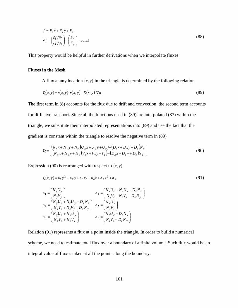
101
const
F
F
yf
xff
FyFxFf
y
x
cyx
=
=
∂∂
∂∂=∇
++=
(88)
This property would be helpful in further derivations when we interpolate fluxes
Fluxes in the Mesh
A flux at any location ( )yx, in the triangle is determined by the following relation
( ) ( ) ( ) ( ) nyxDyxyxnyx ∇⋅−⋅= ,,,, vQ (89)
The first term in (8) accounts for the flux due to drift and convection, the second term accounts
for diffusive transport. Since all the functions used in (89) are interpolated (87) within the
triangle, we substitute their interpolated representations into (89) and use the fact that the
gradient is constant within the triangle to resolve the negative term in (89)
( )( ) ( )( )( ) ( )
++−++++
++−++++=
ycyxcyxcyx
xcyxcyxcyx
NDyDxDVyVxVNyNxN
NDyDxDUyUxUNyNxNQ (90)
Expression (90) is rearranged with respect to ( )yx,
( ) 654321 aaaaaaQ +++++= 22, xxxyyyyx (91)
−
−=
+
+=
=
−+
−+=
−+
−+=
=
yccc
xccc
yxxy
yxxy
xx
xx
yyyccy
xyyccy
yxxccx
xxxccx
yy
yy
NDVN
NDUN
VNVN
UNUN
VN
UN
NDVNVN
NDUNUN
NDVNVN
NDUNUN
VN
UN
63
52
41
aa
aa
aa
Relation (91) represents a flux at a point inside the triangle. In order to build a numerical
scheme, we need to estimate total flux over a boundary of a finite volume. Such flux would be an
integral value of fluxes taken at all the points along the boundary.

102
Figure 50. Triangle with locally indexed vertices, centers of the edges, and normal vectors
We assign an index Nk ...1= to each triangle connected to the vertex of interest. The
centers of triangles receive the same index and become kc . The centers of edges belong to two
triangles (to one triangle - only in the case when the edge belongs to a boundary of the domain);
hence, they cannot be indexed in such a simple manner. Inside a triangle we introduce a local
indexing of vertices. The indices of centers of edges ie and normal vectors in are connected to
vertices, opposite to that edge. The normal vectors are directed in the direction of counting of the
vertices (Figure 50).
The continuity equation for plasma can be written in terms of fluxes with the right-hand
side written in a general form
recgenI
t
n/=•∇+
∂∂
Q (92)
Here Q is the summary of all the fluxes (incoming and outcoming) in the finite volume.
Applying the concept of finite volume approach, we integrate equation (92) over the finite
volume that has an areaA .
∫∫∫ =•∇+∂
∂
A
recgen
AA
dAIdAdAt
n/Q (93)

103
We assume that values of number density, and generation/recombination term at the
vertexv are average values over the whole finite volume associated with the vertex. Thus, they
can be taken out of the integral. We also assume that integration is carried over the finite volume
which consists of combination of smaller volumes contributed by each particular triangle. This
assumption allows us to split the integral over the finite volume into a sum of integrals over each
particular piece of a triangle.
∑∑∫==
==•∇+∂
∂ N
kkvrecgen
N
k Av
AAAIdAAt
n
k1
/1
,Q (94)
Here kA is the area of the sub-volume of the kth triangle. Area of any triangle could be calculated
using Heron’s formula ( ) ( ) ( )2131323212
1yyxyyxyyxA −+−+−= .
According to Divergence Theorem [87] the integral term of equation (94) can be modified as
follows
∫∫ •=•∇
kk AA
dldAδ
QnQ (95)
Here the right-hand side is the integral taken over the boundary of the kth triangle. This integral
could be further split into the sum of integrals over each separate piece of the boundary. As the
example, let us write the integral at the vertex1v for the case shown in Figure 50.
∫∫∫∫∫ •+•+•+•=•
122331 vececeevA
dldldldldl
k
QnQnQnQnQnδ
(96)
If the edges of the triangle do not belong to the boundary of the domain, the integral
terms in (96) over the boundaries 31ev and 12ve would be canceled out due to double integration.
In the neighboring triangles that share the same edges 31ev and 12ve the integration would be

104
taken in the opposite direction, hence, the opposite sign of the integral terms. Therefore, equation
(96) is reformulated accounting for the canceling terms and is substituted into (94).
AIdldlAt
nvrecgen
N
k eccevkkkk
/1
23
=
•+•+
∂
∂ ∑ ∫∫=
QnQn (97)
This is the continuity equation integrated over the finite volume and written in terms of fluxes.
Integration Path in the Mesh’s Triangles
In order to evaluate the integral term of (97) over any set of triangles, we need to find
normal vectors and estimate the fluxes over the boundaries ce3 and 2ce (please, refer to Figure 49.
The calculation of normal vectors is based on the following relations.
0
1
0
13mod <•
=
=•
+i
ii
cen
n
cen
i
i (98)
The last condition in (98) provides proper direction to normal vectors. According to relations
(98), the normal vectors for a triangle are calculated with the following coordinates.
+
+±
=
=
2
2
1
1
1
i
i
i
ce
cei
Cn
CnCn
y
xCn
i
i
m
in
(99)
The vector ice is calculated as follows
( ) ( )
( ) ( )
( )
( )
−+
−+
=
++−
+
++−
+
=+++
+++
++++++
++++++
6
26
2
32
3213mod113mod
13mod113mod
13mod113mod13mod113mod
13mod113mod13mod113mod
iii
iii
iiiii
iiiii
yyy
xxx
yyyyy
xxxxx
ice (100)
As the general approach, we assume that integral of the flux needs to be evaluated over some
linear path in the triangle. The path is determined by coordinates of the end points

105
−
−=
be
be
yy
xxpth (101)
Points
=
b
bb y
xp and
=
e
e
y
xep determine the beginning and the end of the path,
correspondingly. The normal vectors to this path are determined as
+
+±
=
−−
=
2
2
1
1
1
Cn
CnCn
yy
xxCn
be
be
m
n
(102)
Validation of normal vectors confirms the major properties, i.e. their orthogonality and unit
length. The sign of the normal vectors is determined based on specific conditions and depend on
the location of the path. The orientation of normal vectors has a special form at the inner
boundaries of the triangle to simplify summation of the fluxes when contribution at each
particular vertex is estimated. It also could be inner/outer normal to the triangle edge, when the
edge represents the boundary of the domain.
( )
( ) ( )[ ] 0
1
1
11
11
1
1
1
222
22
2
2
=−−±
−
−+
=
−
−+
−
−
−+
−±=
=
−
−+
−−
−
−
−+
−±=
−
−⋅
−
−+
−
−
−
−+
±
=⋅
bebe
be
be
be
be
be
be
be
be
be
be
bebe
be
be
be
be
be
be
be
be
be
be
be
be
xxxx
yy
xx
yy
xx
xx
yy
xx
xx
yy
xx
yyyy
xx
yy
xx
xx
yy
xx
yy
xx
yy
xx
yy
xx
mm
m
m
pthn
(103)

106
1
1
1
11
1
11
1
21
2
2
21
2
2
2
212
2
2
2
=
−
−+
−
−+
=
=
−
−+
−
−
+
−
−+
=
−
−+
−
−
+
−
−+
±=
be
be
be
be
be
be
be
be
be
be
be
be
be
be
be
be
yy
xx
yy
xx
yy
xx
yy
xx
yy
xx
yy
xx
yy
xx
yy
xx
mn
(104)
In the first case, condition (100) may be applied, when vertices of the triangles are
counted clockwise/counterclockwise, the normal vector would be always pointing to the opposite
direction, i.e. counterclockwise/clockwise. In the second case, the normal vector may point in the
direction similar to direction of the vector starting at the vertex, opposite to the considered edge,
and ending at the center of the edge (dot product of the specified vector and the normal vector
should be positive); this condition provides the outer normal. When the integration part is an
arbitrary line inside of the triangle, other conditions may apply to determine direction of the
normal, but in most cases they could be built based on the vertices of the triangle and center
points of the edges and the triangle itself.
The path, in the general case, may be formulated as a function of x or y only.
1 ,
1 ,
>−−
−−
+−−
=
≤−−
−−
+−−
=
be
be
be
ebbe
be
be
be
be
be
beeb
be
be
xx
yy
yy
xyxyy
yy
xxx
xx
yy
xx
xyxyx
xx
yyy
(105)
The flux at any point in the triangle is described by equation (91). This flux must be
integrated over a portion of the boundary of the finite volume to yield with the integral term of
(97). The integration could be accomplished analytically providing with very good accuracy and
computational efficiency, but it requires knowledge on exact path of integration.

107
Figure 51. Integration paths in a triangle
We want to estimate the paths in the triangle along which the integration is carried on.
Let us refer to the interpolation scheme one more time. In terms of interpolation coordinates( )ηξ ,
the important points in the triangle could be written in the following form
( ) ( )( ) ( )( ) ( )
( ) 32
33
22
11
at ,13131
210001
02110
212100
vvc
ev
ev
ev
=+=
==
==
==
ηξ
(106)
Since the coordinates for all necessary points are known, we can estimate a line passing through
two points and apply this method to1ce , 2ce , and 3ce . The following lines are found
[ ][ ]
[ ]( ) [ ]( ) [ ]
[ ]
∈−=
∈−=
∈−=
∈−=
∈=
∈=
21,0 ,21
1,0 ,2/1: line
1,0 ,2/1
21,0 ,21: line
21,0 ,
21,0 ,: line
3
2
1
ηηξξξη
ηηξξξη
ηηξξξη
ce
ce
ce
(107)
We substitute (84) into (107) and obtain integration paths in terms of( )yx, .

108
+
−−+
+
+−=
+
−−+
+
+−=
+
−−+
+
+−=
+
−−+
+
+−=
−
−−
−
−−=
−
−−
−
−−=
ξη
ξη
ξη
ξη
ξη
ξη
ξη
ξη
ξη
ξη
ξη
ξη
ξη
ξη
ξη
ξη
ξη
ξη
ξη
ξη
ξη
ξη
ξη
ξη
XX
CCy
XX
YYx
YY
CCx
YY
XXy
ce
XX
CCy
XX
YYx
YY
CCx
YY
XXy
ce
XX
CCy
XX
YYx
YY
CCx
YY
XXy
ce
2
21
2
222
21
2
2
: line
2
21
2
22
21
2
2
: line : line
3
21
(108)
Relations (108) determines path of integration in the triangle. There are two functions (
( ) bkxxy += and ( ) dmyyx += ) provided for each path, the reason is that the triangle is randomly
oriented in space with path of integration represented by a line – in some cases the line is
perfectly vertical or horizontal. The vertical case is extreme for ( )xy and the horizontal case is
extreme for ( )yx , thus one of the representations could be used, after orientation of the
integration path is determined. The criterion for the path orientation is simple: when 1>k we use
( ) dmyyx += , when 1<=k we use ( ) bkxxy += . The integration over the path requires not only
knowledge on the function describing the path, but also evaluation of the length element along
the path. The following formulation provides an easy way of such an evaluation.
dyLdlmxLdmyx
dxLdlkyLbkxy
xyx
yxy
=+=+=+=
=+=+=+=22'
22'
11
11 (109)
Considering a triangle shown in Figure 51, we would like to introduce three auxiliary
integrals, corresponding to the three paths of integration. We modify integral terms in (96)
eliminating the normal vectors from the integrals, due to the fact that they are constants, and take
only the terms that do not cancel out when integration passes through all the neighboring
triangles.

109
( ) ( )( ) ( )( )
( ) ( )( ) ( )( )
( ) ( )( ) ( )( )∫ ∫∫
∫ ∫∫
∫∫∫
===
===
===
3 33
2 22
111
,,,
,,,
,,,
3
2
e
c
y
y
x
x
x
y
e
c
y
y
x
x
x
y
y
y
x
x
x
y
e
c
e
c
e
c
e
c
e
c
e
c
e
c
dyLyyxdxLxyxdlyx
dyLyyxdxLxyxdlyx
dyLyyxdxLxyxdlyx
QQQI
QQQI
QQQI 1
(110)
Since we know the flux value at any point (91), the length element (109), and the relation
between the coordinates (108) when following the path, we can substitute all this expressions
into (110) and proceed with further evaluation. The evaluation is done for two cases:( ) bkxxy +=
and ( ) dmyyx += . After simple algebraic derivations, the resultant terms are gathered with respect
to ja (the coefficients from (91)). The result could be written as follows.
3...1 ,654321 =+++++= ibbbbbb iiiiii 654321i aaaaaaI (111)
( )( )
( )( )( ) ( )ceixiceiyi
iiiiiceiyi
iiiceiyi
iiiiii
ceixiiii
ceixiiiiii
iiii
yyLbxxLb
bmbmdbdbxxLb
bmbdbxxLb
bmbdbbkbbb
yyLbbkbbb
yyLbbkbkbbbb
dymxbxky
−=−=
++=−=
+=−=
+=+=
−=+=
−=++=
+=+=
66
12
262
533
5
26422
4
123543
222462
3315
246
21
23
2
2
32
The coefficients jib depend only on geometry of the mesh. If the mesh does not change
during the simulation, they remain constants. Before the simulation starts, the analysis of the
mesh takes place: for each triangle of the mesh, orientation of the integration paths is estimated
using the described criterion. The result is the decision on which representation of the path
should be used ( ) bkxxy += or ( ) dmyyx += . According to the used representation, a set of jib is
calculated and stored for the pathi ; thus, a triangle receives three such sets – one for each path.
Whenever the flux along the path needs to be estimated, the coefficients ja are recalculated

110
accounting for new values of number density, velocity, and diffusion coefficient at the vertices of
the triangle. The relation (111) is then used to provide the fluxes along the paths.
One important note should be given. The integration of the fluxes proceeds from the
center of the trianglec towards the edgeie . The sign of the flux iI remains unchanged if the
coordinate of pointc used as parameter of integration is smaller than the corresponding
coordinate of pointie , in the opposite case the sign of iI should be reversed. This estimation may
be performed at the initial stage of the simulation and the sign reversion could be introduced into
jib automatically providing with the proper sign whenever (111) is applied.
The fluxes (111) are associated with the path of integration. In order to determine how
much matter passes over the boundary created by the path lines, the dot product of the auxiliary
fluxes and the corresponding normal vectors should be found. Each triangle contains a sub-
volume of the finite volume element. The sub-volume at the vertex iv is determined by two
boundaries ( ) 13mod1 ++ice and 13mod +ice . We do not account for the boundaries( ) 13mod1 ++ii ev and 13mod +ii ev ,
because positive/negative flux contribution here cancels out by negative/positive contribution at
the neighboring triangle; unless the edge is at the boundary of the domain, which is the separate
case discussed later. Thus, the contribution of the fluxes to the sub-volume at the vertex iv in the
triangle k is determined by fluxes over boundaries ( ) 13mod1 ++ice and 13mod +ice . Based on the direction
of the normal vectors and location of the path lines, the following relation takes place.
11223
33112
221
nInI
nInI
nInI 33
•−•=
•−•=
•−•=
k
k
k
Q
Q
Q
(112)
In this relation, the variable ksQ represents total contribution of the fluxes to the sub-
volume at the vertex sv in the trianglek with 3,2,1=s being a local indexing within the triangle.

111
With modifications provided in (112), the continuity equation (97) is transformed into simpler
version.
AIQAt
nvrecgen
N
kks
v/
1
=+∂∂
∑=
(113)
Equation (113) represents an explicit scheme for iterations of number density at the vertex of
interest.
−∆+= ∑
=
N
kksvrecgenvoldvnew Q
AItnn
1/
1 (114)
Boundary Conditions
In order to properly estimate fluxes crossing the boundary of the domain, we have to
consider an arbitrary flux in a general form, based on the derivations provided for the finite
volumes. Let us assume an arbitrary line which provides a path for the integration.
1 ,
1 ,
>−−
−−
+−−
=
≤−−
−−
+−−
=
be
be
be
ebbe
be
be
be
be
be
beeb
be
be
xx
yy
yy
xyxyy
yy
xxx
xx
yy
xx
xyxyx
xx
yyy
(115)
dyLdlmxLdmyx
dxLdlkyLbkxy
xyx
yxy
=+=+=+=
=+=+=+=22'
22'
11
11
The flux crossing this line at point( )yx, can be written in the following form
( ) 654321 aaaaaaQ +++++= 22, xxxyyyyx (116)
This instantaneous flux is integrated along the considered path yielding with total flux
( ) ( )( ) ( )( )∫∫∫ ===ye
yb
x
xe
xb
y
end
start
pth dyLyyxdxLxyxdlyx ,,, QQQI (117)
Substitute flux (91) into the integrals; also substitute definition of the lines

112
( ) ( ) ( )
( ) ( ) ( ) ∫
∫
∫
++++++++=
++++++++=
=+++++=
ye
yb
x
xe
xb
y
end
start
pth
dyLdmydmyydmyyy
dxLxxbkxxbkxbkx
dlxxxyyy
654321
654321
654321
aaaaaa
aaaaaa
aaaaaaI
22
22
22
(118)
This equation provides results for both representations of the integration path ( )xyy = and
( )yxx = . We simplify this integral and gather the terms in front of coefficients ia
( ) ( ) ( )
( ) ( ) ( ) ∫
∫
+++++++++
+++++++++
ye
yb
x
xe
xb
y
dyLdmdyymdmydymyyy
dxLxxbxkxbkxbbkxxk
654321
654321
aaaaaa
aaaaaa
22222
22222
2
2
(119)
Since coefficients ia are determined only from the nodal values and do not depend on the
coordinates, they can be taken out of the integral together with the length correction which is
constant for the whole integration path.
( ) ( )
( )
( )
( ) ( ) ∫∫∫
∫∫∫
∫∫∫∫
∫∫
++++++
++++
+++++
+++++
ye
yb
x
ye
yb
x
ye
yb
x
ye
yb
x
ye
yb
x
ye
yb
x
xe
xb
y
xe
xb
y
xe
xb
y
xe
xb
y
xe
xb
y
xe
xb
y
dyLdydmdyymLdydmyL
dydymyLydyLdyyL
dxLdxxLxdxLdxbxkxL
dxbkxLdxbbkxxkL
654
321
6543
21
aaa
aaa
aaaa
aa
222
22
22
222
2
2
(120)

113
We evaluate the integrals
( )
( )yeybx
ye
yb
x
ye
yb
x
ye
yb
x
ye
yb
x
ye
yb
x
xexby
xe
xb
y
xe
xb
y
xe
xb
y
xe
xb
y
xe
xb
y
yLydy
mdy
mLdyy
mL
yd
ymL
yL
yL
xLx
Lx
Lx
bx
kL
bxx
kLxbx
bkx
kL
654
321
6543
21
aaa
aaa
aaaa
aa
+
+++
++
+
++
+
+
+
+
++
+
++
++
223
22
2323
3223
22
232
22
32
2323
3223
222
3
(121)
Then, estimate the general form of the coefficients to formulate the flux
( ) ( )
ye
yb
x
ye
yb
x
ye
yb
x
ye
yb
x
ye
yb
x
yeybx
xe
xb
y
xe
xb
y
xe
xb
y
xe
xb
y
xe
xb
y
xexby
pth
yLb
yLb
yd
ymLb
dyy
mLb
ydy
mdy
mLb
yLb
xbx
bkx
kLb
bxx
kLb
xb
xkLb
xLb
xLb
xLb
bbbbbb
=
=
+=
+=
++=
=
++=
+=
+=
=
=
=
+++++=
3
2
23
2
22
3
22
3
2
23
2
3
3
1
2
2
23
3
2
4
223
25
6
223
21
2
2
23
3
2
4
3
5
6
654321 654321 aaaaaaI
(122)
Depending on the type of representation used for the integration path, there are two results
obtained

114
( )
( )( )
( )
( )
( )bex
bex
bex
bey
bey
bey
pth
yyLb
bdmdbbmb
dbmbb
dbmbb
yyLb
yyLb
xxLb
xxLb
xxLb
bbkbb
bbkbb
bbbkbbkb
bbbbbb
−=
++=
+=
+=
−=
−=
−=
−=
−=
+=
+=
++=
+++++=
6
62
212
5
624
213
222
331
6
335
224
453
642
62
452
1
654321
2
2
13
1
3
12
1
2
654321 aaaaaaI
(123)
The flux crossing the considered edge is found by projection of the total flux on the normal
vector calculated for the edge
pthpthpthQ nI •= (124)
The sign of the crossing flux depends on the direction of the normal, which could be either
positive or negative, depending on the considered vertex.
Figure 52. Convective transport of plasma species using central difference scheme only
Figure 52 shows the typical result for a calculation based on the central difference
scheme for convective transport of the species. The “saw” effect is severely pronounced for both
species. The peak value of the number density in both cases is [ ]317 m1105.3 × which is higher
than the original maximum number density. The “saw” distribution of plasma species leads to

115
very high peaks and very deep valleys between the peaks. The species accumulated at the peaks
result with high values of the number density.
Upwind Descritization
The method presented in the previous section resembles central difference scheme, which
is known for introduction of unphysical oscillations when convective transport is considered.
The oscillations lead to instabilities and poor convergence of the solution. In order to resolve the
instability, the upwind descritization is applied to the problem. The value of the number density
at the interface between two adjacent finite volumes is determined based on the velocity field.
The velocity components are interpolated at the interface using simple geometric interpolation. A
triangle is considered in order to estimate the interfacial parameters. The parameters (velocity,
diffusion coefficient, and number density) are calculated at the center of the triangle and at the
centers of its edges. Next, these parameters are calculated at the centers of the lines connecting
triangle’s center and edges’ centers; the same lines represent the interfaces between adjacent
finite volumes. The number density at the interface is calculated at this time for further use in
central difference descritization. The interfacial velocities are multiplied by normal vectors at the
interfaces to evaluate the overall impact of the flow on each of six sub-elements forming finite
elements at the triangle. The sign of this multiplication determines which vertex lies upwind
relative to the considered interface. The number density value and gradient of number density at
the upwind vertex are used in the form of Taylor-series expansion to evaluate the number density
at the interface. This newly evaluated number density is different from the one previously found
in accordance with geometrical interpolation. The former includes more information about
incoming flow which usually increases the interfacial number density.

116
The gradient of number density at the vertices of the triangle requires a special procedure
for accurate calculation. The method that we use in our model is targeted to minimization of the
gradient error in the least-squares sense; thus, it has a name of Least Squares Linear
Reconstruction Method [88]. The idea of the method is relatively simple. We consider one
computational node on the domain. In the general case, this node belongs to multiple triangles
and is surrounded by multiple vertices which share same edge with the considered node. We may
estimate a gradient between two nodes using ().
( )xxxx
−−
−=∇ i
i
ii
nnn
2
(125)
This gradient is specific for the node i, when applied to other nodes it would result with
sufficient error. If we cycle through all the surrounding nodes and calculate algebraic average of
the gradient, we would find the first approximation to the gradient at the considered node. To
increase the accuracy of gradient calculation, we represent the error in the form of the least
squares minimization problem
( )( )[ ] min1
2
12
→−∇+−−
∑=
Nsur
iii
i
nnn xxxx
(126)
In this representationn∇ stands for the gradient that results in the smallest overall error
when applied to any surrounding node. This gradient needs to be found from the solution of the
minimization problem.
( )( )( )[ ] 0
1
1
2
2=
−∇+−
−∇∂∂
∑=
Nsur
iii
i
nnnn
xxxx
(127)
( )( )[ ]( ) 01
2 T
12
=
−−∇+−
−− ∑
=
xxxxxx
i
Nsur
iii
i
nnn

117
( )( ) ( )( )[ ] 01
1
T
2=−−∇−−−
−∑=
Nsur
iiiii
i
nnn xxxxxxxx
( )( )[ ] [ ]∑∑==
−∇−
=−−−
Nsur
ii
i
Nsur
iii
i
nnn1
2
21
2
11xx
xxxx
xx
(128)
( )( )[ ]∑=
−−−
=∇Nsur
iii
i
nnNsur
n1
2
11xx
xx
The upwind numerical scheme improves the overall stability of the simulation, at the
same time it introduces significant numerical diffusion. This is why the upwind scheme is
usually blended with other numerical schemes (the central difference scheme, for example). Such
combination is advantageous in both, stability and diffusion domains.
Figure 53. Convective transport of plasma species using upwind difference scheme only
Figure 53 represents the effect of upwind scheme when applied to 2D convective
transport problem. In this simulation, a parabolic profile of longitudinal velocity and zero
transverse velocity were applied. The species are expected to fill the whole domain using the
initial distribution as a pattern. The numerical diffusion can be noticed when initial distribution
of species number density (on the left side of either plot in Figure 53) is compared to that at the
end of the channel (on the right side of the plots). The diffusion is so excessive, that this scheme

118
yields unphysical representation of the plasma and cannot be utilized alone to produce accurate
results.
Blending
The two numerical techniques can be blended with arranging them into a linear
combination, to determine the interfacial value of the conserved variable, in accordance with the
following equation
( ) CENTRALUPWINDf nnn αα −+= 1 10 ≤≤α (129)
The blending coefficient α can be used as a constant for the whole simulation. The results of
such blending are represented in Figure 54.
Figure 54. Blending of the numerical schemes with different blending coefficientsα

119
Figure 54 represents static blending of Central and upwind numerical schemes. The
following cases take place: 0=α is pure central difference scheme, 10 <<α is blended
numerical scheme, and 1=α is pure upwind numerical scheme. In the shown result for 25.0=α
central difference scheme dominates. The distribution of the species is significantly smoothened
by partial contribution of upwind scheme, but smaller scale instabilities are still present, though
the result is not as dramatic as the one calculated for 0=α (Figure 52). The case 5.0=α may
be considered the best of the presented four cases. The instability due to central difference
scheme is hardly noticeable; at the same time, the numerical diffusion did not develop
sufficiently to excessively smoothen the data at the outlet. In both cases 75.0=α and 1=α the
domination of upwind formulation determines significant smothering of the species profiles at
the whole domain; thus, 5.0>α is not a good factor when physical consistency is a concern.
As it can be concluded, the static application of the blending factor does not produce
satisfactory results. This is why we develop and use dynamic blending. In dynamic blending the
blending factorα is determined specifically for each particular part of the boundary of the
considered finite volume. The algorithm for dynamic calculation of α is relatively simple.
Figure 55. Calculation of dynamic blending factor

120
Let us consider an example shown in Figure 55. We assume that the interfacial value of
number density at the pointp has to be found, we also assume that the flux is directed left-to-
right with the highest value at the vertex1v . Next, we extrapolate the velocity vector at the point
p following the upwind direction, until it intersects one of the triangle’s edges. The green,
orange, and red lines in Figure 55 represent such an extrapolation, with the points 321 ,, ppp
indicating the intersection with the edges. The major edges for the finite volumes at vertices 0v
and 2v are 2e and 0e , specifically the portions 20ev and 02ev . When a line intersects the edge 1e
(the red line with the intersection point 1p in Figure 55), the interfacial number density is
severely affected by the vertex0v ; therefore the blending factor is 1=α . Intersection with the
edge 2e above the center of the edge (green line with the intersection point 3p in Figure 55)
indicates that the effect of the center of the edge is dominant, thus the central difference scheme
is used with the blending factor 0=α .
Figure 56. Dynamic blending results
The blending factor is between zero and one, when the line intersects the major edge at
the proper half (the orange line with the intersection point 2p in Figure 55). In this case, the

121
blending factor is determined as 2022 evep=α , which estimates the proper contribution of
both of the scheme, based on the proximity of the extrapolated point to the center of the edge or
the upwind vertex. The results calculated with dynamic blending (Figure 56) provide higher
accuracy in comparison to those calculated with either of the numerical scheme alone.
The combination of central difference and upwind numerical schemes yields with
relatively good number density profiles. Compared to the best static case ( 5.0=α ) the
numerical diffusion is slightly smaller, especially when comparing data at the outlet: orange-
yellow color in the static case (Figure 54) versus red-yellow in the dynamic case (Figure 56).
The instability due to the central difference scheme is still present. In order to estimate the work
of the dynamic blending we calculate the mean α , as the average value of all the blending
factors calculated on the domain within one particular iteration. The data presented in Figure 56
are acquired within 100000 iterations; thus, a set of 100000 alphas was recorded. The mean
blending factor fits into the range ( )0.38881950.3883498, , with the average of the factor being
0.388816.
The possible improvement for the dynamic blending may be achieved by using cell-
centered finite volumes, as they provide more uniform distribution of the finite volume sixe and
orientation.
Solution of Poisson Equation
The solution of Poisson equation requires a special numerical algorithm that is suitable
for the unstructured meshes. There are different approaches used for solution of Poisson-based
problems [89, 90]. Some researchers map the nodal values of the unstructured mesh to a regular
mesh, solve the problem on the regular mesh using the “cross-pattern” for descritization of the

122
second derivative, and map the result back to the unstructured mesh. This approach does not
provide any benefits and does not validate the use of unstructured mesh, as the evaluation could
be performed on the regular mesh right away. Some other methods use Fast Fourier Transform
[91] which can be very well parallelized [92] or Fast Multi-pole approach [90, 93]. The accuracy
of the solution may be substantially improved by addition of Multigrid algorithm [94-96]. In this
work we propose a novel method for descritization of Poisson problem on unstructured meshes.
Figure 57. The shortest distance in a triangle from the vertex of interest to: (a) the opposite edge, (b) the closest vertex on the opposite edge, (c) horizontal edge, (d) vertical edge
The novel method is based on involvement of all the neighbor nodes into the calculation
at the considered node. Each triangle connected to the considered node provides with a specific
contribution to the function evaluated at the node. The contribution coming from a connected
triangle is scaled according to the size of the triangle in terms of the angle span measured from
the node of interest. The contribution of each particular triangle is determined at a specific

123
distance mr from the considered node. This distance is evaluated as a fraction of the smallest
distance between vertices and edges of the triangles in the whole mesh.
Assume that we are located at vertex 1v and we want to find the shortest distance between
the current vertex and the opposite edge32vv . If we are currently at another vertex, let’s change
the local indexing and denote the current vertex with index 1, the position of other two vertices
does not matter. The shortest distance represents a line either connecting 1v with a point pon the
opposite edge of the triangle (Figure 57.(a)) or connecting 1v with one of the other two vertices
(Figure 57.(b)). There are two cases that could be handled without extra calculations – when the
opposite edge is horizontal (Figure 57.(c)) the closest point is ( )21 yxp = and when the opposite
edge is vertical (Figure 57.(d)) the closest point is ( )12 yxp = .
In the general case (Figure 57.(a)) the closest point is calculated using two equations
which are determined from the fact that vectors pv1 and 32vv are perpendicular and the point p
belongs to the edge 32vv .
The solution (130) represents the case when the edge 32vv has a shallow slope. When the
slope is steep, it is reasonable to handle the edge equation as dmyx += , the solution transforms
accordingly
( )( ) ( )( )
−
−+
−
−=
=−−+−−
23
2332
23
23
231231 0
xx
xyxyx
xx
yyy
yyyyxxxx
pp
pp
( )
−
−=
−
−=
+=
−++
=
23
2332
23
23
1121
1
xx
xyxyb
xx
yyk
bkxy
kbkyxk
x
pp
p
(130)

124
( )
−==
−++
=
+=
kbdkm
mdmxym
y
dmyx
p
pp
11
1112
(131)
Since the orientation and the shape of the triangle are arbitrary, the distance ( )pvl ,1 should be
compared to( )21, vvl .
The general form of Poisson equation for electrostatic case reads
ε
ρϕϕ f
f −==∇•∇=∆ (132)
Here ϕ is a scalar electric potential, fρ is free charge density, and ε is electrical permittivity of
the media. The formulation especially useful for our application is written as follows.
fyyxx
=
∂
∂
∂
∂+
∂
∂
∂
∂ ϕϕ (133)
Using unstructured mesh we would like to develop a numerical scheme for calculation of
electric potential at the node of interestv . The usual approach to equation (133) on a regular
mesh is to use cross-shaped pattern for finite difference to represent the second derivative of the
potential.
On unstructured mesh, the nodes do not automatically fit into the cross pattern. A
common way to handle this issue is to interpolate values of electric potential from neighboring
nodes such as they lay exactly in the cross-pattern [94]. This method works well at the inner
parts of the computational domain, but, approaching the boundary, the interpolated values may
appear outside of the domain. This is especially true when the boundary is intensively curved.
We utilize the idea of the cross-pattern and apply it to the unstructured mesh at the same time
developing it even further. The cross-pattern assumes that the lines of the pattern coincide with
the coordinate axis of the Euclidian coordinate system. The regular differentiation is

125
accomplished along the pattern lines in the direction corresponding to the positive direction of
the coordinate axis.
Figure 58. Cross-pattern for finite difference representing Laplace operator in Poisson equation
Let us assume that there are some arbitrary nodes which lay on a circle of radius mr
around the node of interest (Figure 58). The value of electric potential at the node of interest is
ijϕ , the values of the arbitrary nodes, forming the cross-pattern are 1111 ,,, +−+− ijijjiji ϕϕϕϕ . The cross
pattern can be written as follows
−−
−+
−−
−=
∂
∂
∂
∂+
∂
∂
∂
∂ −+−+
m
jiij
m
ijji
mm
ijij
m
ijij
m rrrrrryyxx
1111 11 ϕϕϕϕϕϕϕϕϕϕ (134)
Now let us imagine that the coordinate system is rotated at a small angle, becoming a coordinate
system( )',' yx (Figure 58). Since the cross-pattern lines are aligned with the coordinate axis, the
pattern in new coordinates appears to be rotated at angleθ in comparison to the original
orientation. Nevertheless, the same equation (134) is valid in new coordinates. The derivatives of
electric potential with respect to 'x and 'yare taken along the new coordinate axis. We would like

126
to generalize this case: for any angleθ , the cross-pattern (134) properly defines Laplace operator
with differentiation carried out along the new/rotated coordinate axis.
For the observer at the original coordinate system it would appear that differentiation is
taken in “radial” direction with 90o difference in angular direction for x∂∂ and y∂∂ . Moreover,
for o90=θ we have the following relations 2222 ' yx ∂∂→∂∂ and 2222 ' xy ∂∂−→∂∂ . The second
derivative does not change sign ( )( )222222 '' xfxfxfxf ∂∂=∆−∆=∆∆=∂∂ when direction of
differentiation is reversed. We introduce new function ( )yx,ψ which represents the first derivative
of ( )yx,ϕ when taken to the right or to the top of the node of interest, and the first derivative with
the negative sign when taken to the left or to the bottom of the node of interest. Numerically, this
function is calculated like
m
ijijij
m
ijijij
m
ijjiji
m
ijjiji
rr
rrϕϕ
ψϕϕ
ψ
ϕϕψ
ϕϕψ
−=
−=
−=
−=
++
−−
++
−−
11
11
11
11
(135)
We substitute (135) into (134) and obtain
( ) ( ) ( )11111111111
−+−+−+−+ +++=+++=
∂
∂
∂
∂+
∂
∂
∂
∂ijijjiji
mjiji
mijij
m rrryyxxψψψψψψψψ
ϕϕ (136)
Since the sign of the function ( )yx,ψ depends on its location relative to the node of
interest, the mismatch in sign at o90=θ disappears when regular derivatives are substitute with
this function. We can rewrite the Poisson equation in terms of the finite difference, using (136)
( ) ijijijjijim
fr
=+++ −+−+ 11111
ψψψψ (137)
Since the cross-pattern (137) is valid for any angleθ , we want to summarize all such
equations taken at angles [ ]2,0 πθ ∈ . The summation is represented by an integral with respect to

127
the angle θ and evaluated over the interval[ ]2,0 π . There is no reason to take larger interval, as
for 2πθ > the function ( )yx,ψ repeats.
∫∫∫∫∫ =+++ −+−+
2
0
2
0
1
2
0
1
2
0
1
2
0
1
πππππ
θθψθψθψθψ dfrdddd ijmijijjiji (138)
The function ( )yx,ψ is determined on the circle with radius 2mr and changes with angle
θ . Therefore, instead of ( )yx,ψ we can write ( )θψ .
Figure 59. Finite difference for Poisson equation on unstructured mesh
Let us substitute this correction into (138) we keep the integral terms at the same places
on the left- hand side so that the substitution is easy to track back to the original form.
( ) ( ) ( ) ( ) ijm frdddd πθθψθθψθθψθθψπ
π
ππ
π
π
π2
1232
0
2
232
=+++ ∫∫∫∫
( ) ijm frd πθθψπ
2
12
0
=∫ (139)

128
Next, we assume that ( )θψ may be constant in some interval[ ]kk θθ ,1− . If we divide the circle
where ( )θψ is calculated into a set of such intervals, the integral (139) splits into a series of
integrals over the intervals of constant values. Using the fact that ( )θψ is constant in each
interval, it can be taken out of the integral (140).
Figure 59 shows elements of an unstructured mesh connected to a vertex (the black point)
where electric potential should be evaluated. The constant values of ( )kθψ are taken at the circle
of radius 2mr , the angular element kδθ corresponds to the angle of the kth triangle at the vertex of
interest.
( ) ( ) ( ) ( )( ) ijm
N
kkkk
N
kk
N
kk frddd
k
k
k
k
πθθθψθθψθθψθθψθ
θ
θ
θ
π
2
1
11
11
2
0 11
=−=
== ∑∑ ∫∑ ∫∫=
−==
−−
( ) ijm
N
kkk frπδθθψ
2
1
1
=∑=
(140)
It is good to place ( )kθψ at specific coordinates ( )ηξ , in the triangle, for example on the
median connecting the vertex of interestiv and the pointie at the middle of the opposite edge of
the triangle (please refer to interpolation in triangle in the previous section). This way the
coordinates are fixed and location of ( )kθψ is approximately at the center of the angular segment
kδθ . The radius mr could be estimated as the half of the mean distance between the vertex of
interest and all the surrounding vertices.
The advantage of such a modified numerical scheme for Poisson equation is that all
vertices surrounding the vertex of interest contribute to the calculation process. When regular
cross-pattern is used, there are only four points interpolated to fit the pattern. For the example
presented in Figure 59, these points would fit into triangles 2, 3, 5, and N-1. The other
surrounding triangles do not contribute into the calculation process. From one perspective this

129
saves calculation time, because only four interpolations are required. From another perspective,
the information of electrical potential distribution is not complete at the vertex of interest, as
some surrounding vertices did not contribute with their values.
In the Poisson Scheme we assumed that the integral (140) could be integrated over
intervals of constant( )kθϕ . In the simplest case, the constant value has to be taken at the median
connecting the vertex of interest with the opposite edge. The position of the sample point at the
median is determined by radiusmr . The coordinates of the sample point are
( )( ) ( )
( )( ) ( )2132
2132
1321
2132
2132
1321
22
2
22
2
yyyxxx
yyyryy
yyyxxx
xxxrxx m
km
k−++−+
−++=
−++−+
−++= (141)
For better accuracy, the function ( )θϕ has to be integrated from 1−kθ to kθ along the circle
with the center at 1v and radiusmr .The integration result needs to be averaged over( )1−− kk θθ .
Such value would represent the true mean constant value in the triangle.
We assume that electric potential ( )321 ,, ϕϕϕ is known at the corners of the triangle. The value at
the sample point could be interpolated using (86).
( )( ) ( )( ) ( )
( ) ( ) ηξ
ηξ
ηξ
ϕϕϕϕϕ
ϕϕϕϕ
ϕϕϕϕ
ϕ
CC
YY
XX
yxyx
c
y
x
ckykxkk
12131
1213
1213
,
−+−+=Φ
−+−=Φ
−+−=Φ
Φ+Φ+Φ=
(142)
The coefficients of the Poisson Scheme are assembled using coefficients in front of( )321 ,, ϕϕϕ .
We expand (142) and derive the coefficients:
( )
ξξξ
ηηη
ξ
η
ϕϕϕϕ
CyYxX
CyYxX
yx
kkk
kkk
kk
++==Φ
++==Φ
Φ−Φ−=Φ
Φ+Φ+Φ=
3
2
321
332211
1
,
(143)
The same result could be obtained using (84) and (85)

130
( ) ( ) ( ) 3211 ffff ξηηξ ++−−=
We proceed further and calculate coefficients of function ( )θψ . Accounting for (135) we can
write
( ) ( )( )ijmr
ϕθϕθψ −=1 (144)
Substitute (143) into (144)
( ) ( )
( )ikim
i
ijm
r
r
δ
ϕϕϕϕϕϕϕθψ
−Φ=Ψ
Ψ+Ψ+Ψ=−Φ+Φ+Φ=
1
1332211332211
(145)
Here ikδ is the Kronecker delta and k is the local index of the vertex of interest in the considered
triangle. We substitute (144) into (140) and obtain modified coefficients
( ) ijm
N
kkkkk frπδθϕϕϕ
2
1
1332211 =Ψ+Ψ+Ψ∑
=
(146)
The index k in equation (146) passes through all the triangles surrounding the vertex of interest.
The index i at the coefficients iΨ and electric potentialkiϕ corresponds to the exact local index in
the trianglek . The coefficients iΨ can be used only for one vertex in the triangle. If another
vertex is considered, the coefficients must be recalculated, as the median would change with
consequent change in position of the sample point( )kk yx , .
Let us assume that the vertex of interest is surrounded by vN other vertices. We can
rewrite (146) in terms of these vertices
( ) mfskskiks
ijfs
Nv
ss
N
kks
rCC
fCC
πλδθ
ϕ
2
11 1
=Ψ=
=
∑ ∑= = (147)

131
In equation (147) the index spasses through a number of vertices that includes the vertex
of interest and the surrounding vertices directly connected to the vertex of interest, the index k
passes through all the surrounding triangles, the index i is the local index of the vertex s in the
triangle k , the function ksλ is equal to one if the vertex s belongs to the triangle k , otherwise it is
equal to zero. We further simplify (146)
∑−
=
−=1
1
Nv
sssijf CfC ϕϕ (148)
Here ∑=
=N
kkss C
CC
1
1 represents the inner summation and CCC fsf = is a coefficient in front of the
free charge. Both of these coefficients account for the coefficientC in front of the vertex of
interest. It is worth to mention that all considered coefficients depend on geometry only. If the
mesh does not change, they stay constant throughout the simulation. Thus the coefficients could
be calculated at the initial stage and stored in a list which order corresponds to the order of the
vertices surrounding the vertex of interest. When solution of Poisson equation is required the
coefficients are multiplied by corresponding electric potential and, according to (148),
immediately provide the proper value at the considered vertex.
The implicit scheme can be easily derived from (148) resulting with a constant matrix
(unless the mesh changes). This matrix could be processed before the simulation, in order to find
its inverse form. At the simulation, only the right hand side vector consisting of the free charges
needs to be formed. A simple multiplication by the inverse matrix immediately yields with the
correct distribution of electric potential. Even simpler way to find the mean value of ( )θϕ is to
take the mean electric potential at the center of the triangle ( )3213
1ϕϕϕ ++ and to use it for any
vertex assuming that this value is actually on the circle with radiusmr .

132
In order to estimate the effect of the fringing electric field and the species charge on a
solution of the Poisson equation, we calculate and plot (Figure 60) the left-hand side and the
right-hand side of equation (133). According to our analysis, the solution is not affected by
species charges (the right plot in Figure 60); it mainly depends on the fringing electric field (the
left plot in Figure 60) from the electrodes, as it is indicated by seven orders of magnitude
difference between the left and the right hand sides of the Poisson equation.
Figure 60. The left-hand side (left) and the right-hand (right) side of Poisson equation
Figure 61. Electric potential (left) and reduced electric field (right)

133
Figure 62. Electric field components: Ex (left) and Ey (right)
The left plot in Figure 61 represents the electric potential calculated with the use of the
presented numerical scheme. The electric potential at the inlet (Figure 63) is derived from the 1D
model of plasma generation. Due to significant contribution of the fringing electric field, the
highest electric potential for 2D problem is found in the vicinity of electrodes. The further from
the inlet, the lower becomes the electric potential. The electric potential almost does not change
during the simulation due to negligible contribution of species charge to electric potential
distribution. The x- and y-components of electric field (Figure 62) are determined from the
gradient of electric potential.
The steep electric gradient along the inlet, especially in the vicinity of the walls (Figure
63), is a derivative of the oscillating electric field between the electrodes. The y-component of
the electric field is constant, due to the strict relation between 2D and 1D plasma models. At the
same time, the longitudinal component of the field is not bound to 1D problem. In 1D case, this
component was zero, because everywhere between the electrodes, the electric field fluctuated
uniformly. At the channel with free walls, the electric field rapidly changes in x-direction. This is
why the relaxation of electric potential along the channel can be observed even at the inlet.

134
Comparing orders of magnitude, the transverse component of electric field is 2x larger than the
longitudinal one.
Figure 63. Electric potential at the Inlet
The right plot in Figure 61 shows the reduced electric field which is calculated as the
length of the electric field vector divided by the number density of the neutral gas. The reduced
electric field is not constant at the inlet: while the y-component of the field is constant, the x-
component changes accounting for electrical conditions of open channel right after the inlet.
Because the reduced electric field is determined from the length of the electric field vector, its
value constantly changing, following the x-component of the field. The high values of the
reduced electric field in the left-top and left bottom corners correspond to similar behavior of Ey,
leading to well pronounced species generation at these areas of the domain.
There are analytical [93, 97] and numerical [98-100] approaches exist to solve Poisson
equation in order to estimate the fringing effect of the electric field at the edges of the capacitor-
type arrangement of the electrodes. Our model automatically accounts for the fringing effect,

135
using the initial 1D distribution of the electric potential, and expanding it along the channel. Due
to this fact, there is no need for additional procedures to implement the fringing electric field in
the 2D model.
Results and Discussion
The results acquired from 2D simulation of plasma advection in the channel may be
divided into three categories – convective results, electrical results, and the ones combining both,
fluidic and electrical effects. The first category represents plasma species advancing along the
channel due to purely convective forces with no electrical field engaged. For convective
transport, the species may be considered as a regular gas which flows due to the imposed
velocity field. Species distribution due to convective transport is shown in Figure 56. The species
distribution follows velocity profile of the gas flow, resembling parabolic shape. These data do
not properly represent the plasma, as there is no collective behavior of the species when electric
field is taken out of the consideration. Nevertheless, the species distribution is calculated based
on their profile taken from the 1D problem of plasma generation. The next step is introduction of
electric field that is shown in Figure 61 and calculation of the species respond to the field. We
implement the recombination of electrons and positive ions, in order to properly account for the
species losses. Electrons are present at the Inlet in smaller number than positive ions, this is why
they are completely consumed in the recombination process, showing no propagation in the left
plot of Figure 64.
The right plot of Figure 64 represents propagation of positive ions along the channel of
the plasma reactor. The recombination process consumes a majority of positive ions within a

136
short distance, with the peak population falling from [ ]317 1108.1 m× to [ ]317 1104.0 m× , resulting
in 4x decrease in the number density at the distance of cm 1 .
Figure 64. Convective flux of species at the steady state
The species generation and accounting for drift velocity introduces fluxes of few orders
of magnitude higher than those generated by convective transport. These fluxes require
extremely small time step to be resolved correctly by either presented numerical scheme. This
case requires additional treatment that works with large gradients of number density.
Comparing the prediction of 1D plasma model for plasma fade, we can conclude that in
1D case the remaining number density is underestimated. For example, Figure 37 shows
[ ]315 110776.1 m× as the number density for remaining positive ions at the distance of cm 1 ,
which is 20x smaller than the value predicted by 2D model.
Figure 65 shows typical profiles for number density of positive ions measured with
mm 2 step, starting from the Inlet. The drastic decrease in number of ions could be immediately
seen when the profile at the Inlet (mm 0 ) and the one at mm 2 are compared. The very
pronounced feature of all the profiles, except the initial one, is a depression at the center which is
formed due to the recombination process. Since the recombination term is directly proportional

137
to the number density of the species, the highest species loss occurs at the central area where the
largest number of the species is present. Electrons are consumed in this process entirely, while
positive ions develop a depression in their number density profile.
Figure 65. Typical profiles of advected plasma at different locations along the channel
Figure 66. Average blending coefficient for dynamic blending of 2D numerical scheme

138
The data presented in this section is calculated using 100000 iterations on a
computational domain consisting of 2500 nodes connected into 4752 triangular elements that
compose the mesh. The dynamic blending favored central difference scheme spending most of
the time around 3788.0=α (Figure 66). A similar value of the blending factor was observed for
random unstructured mesh and for the mesh with triangles having two sides aligned with the
coordinate axes.

139
CONCLUSION
The model of plasma discussed in this work has been known for few decades. However,
some features of this model were not clearly understood. In this work we highlighted the details
that we found important or challenging while simulating plasma behavior, for example, we found
how the boundary conditions have to be properly constructed for a numerical representation of
1D Poisson equation, we observed major species generation at locations different from the peaks
of number density, we also developed two numerical approaches to solution of convective
transport and the Poisson equation in 2D case.
For the 1D problem of plasma generation between two parallel electrodes, we discussed
time-averaged profiles of number density of the species, the electric field, the
generation/recombination, the temperature of species, and some other parameters evaluated in
numerical simulation. These parameters provide the necessary initial conditions for the 2D
model of the LAPPD system. The analysis of these parameters emphasized important features
and revealed previously hidden relations among processes in plasma.
The surface plots presented in the work help with understanding of some dynamic effects,
such as when and why the generation/recombination happens. Some results lead to interesting
outcomes. For example, it is easy to imagine that generation of species should happen when a
large cloud of electrons passes through a neutral gas. Nevertheless, the surface plots showed that
the major generation happens at the point where number density of electrons is closer to the
mean value, with high electric field generated due to overhead of ions at that location. The
surface plots also provided visual assistance in understanding dynamics of plasma motion in the
alternating electric field.

140
Plasma sheath and phase shift were considered as potential parameters for experimental
measurements, creating a good validation point for the model of plasma generation and
sustainment. Finally, some engineering outcomes were made from the model of plasma
generation. Temperature of electrodes was represented as a function of applied external voltage
and analyzed with considerations on the necessity of cooling equipment. The interesting example
of plasma fade showed a potential range of plasma plume. The range was estimated for different
voltages in order to roughly determine the favorable mode of operation for the LAPPD setup.
In the 2D model we developed two numerical methods in order to simulate plasma on
unstructured meshes. One method addresses solution of continuity equation for plasma species,
using the concept of finite volumes and analyzing fluxes crossing the boundaries of the finite
volumes. Analytical derivations and numerical results are present in this work to demonstrate
this method. The second method was developed for solution of Poisson equation on unstructured
meshes. When calculating electric potential at one of the nodes, the method naturally involve all
the surrounding nodes into the calculation, with each node contributing to the result according to
the angular span of the triangle that contains both nodes – the one that is subject for potential
evaluation and the one contributing with its potential. This method requires only minor
derivations on based on the geometry of the given mesh. If geometry does not change, the
method allows creation of a constant matrix and, possibly, finding its inverse form for very fast
and accurate solution of Poisson problem.
Numerical results acquired for 2D problem of plasma advective transport along a channel
representing the linear plasma head, showed typical distribution of plasma species for the case of
pure convection, as well as for the case of recombination. The length of the plasma plume and
average number density of plasma species are found to be underestimated in the case of 1D

141
plasma fade. The 2D model introduces corrections into the expected profiles of number density
taken at different distance from the outlet of the generation chamber.

142
REFERENCES
1. A. E. Koniges, “Industrial Strength Parallel Computing”, 2000, Morgan Kaufmann Publishers,
San Francisco
2. M. A. Lieberman, A. J. Lichtenberg, “Principles of plasma discharges and materials
processing”, 2nd Ed, 2005, Wiley-Interscience, Hoboken, NJ.
3. K. W. Johnson, “Atmospheric pressure plasma enhanced chemical vapor deposition : design
and application”, Thesis, Mechanical Engineering Department, North Dakota State University,
2011, Fargo, ND.
4. A. Sarani, A. Nikiforov, N. De Geyter, R. Morent, C. Leys, ., “Characterization of an
atmospheric pressure plasma jet and its application for treatment of non-woven textiles”,
Proceedings of 20th international symposium on plasma chemistry, 2011.
5. A. Bogaerts, E. Neyts, R. Gijbels, J. van der Mullen, “Gas discharge plasmas and their
applications”, Spectrochimica Acta Part B-Atomic Spectroscopy, 2002, 57(4), pp. 609-658.
6. A. A. Fridman, “Plasma chemistry”, 2008, Cambridge University Press, Cambridge, NY.
7. S. Z. Li, J. P. Lim, J. G. Kang, H. S. Uhm, “Comparison of atmospheric-pressure helium and
argon plasmas generated by capacitively coupled radio-frequency discharge”, Physics of
Plasmas, 2006, 13(9)
8. I. A. Kossyi, A. Y. Kostinsky, A. A. Matveyev, V. P. Silakov, "Kinetic scheme of the non-
equilibrium discharge in nitrogen-oxygen mixtures", Plasma Sources Sci. Technol., 1992, 1, pp.
207-220
9. J. M. Stillahn, K. J. Trevino, E. R. Fisher, "Plasma Diagnostics for Unraveling Process
Chemistry", Annu. Rev. Anal. Chem., 2008, 1, pp. 261–291
143
10.D. Orlicki, V. Hlavaceky, H. J. Viljoenz, "Modeling of a-Si : H deposition in a DC glow
discharge reactor", Journal of Material Research, 1992, 7(8), pp. 2160 - 2181
11 G. Chen, “Nanoscale Energy Transport and Conversion”, 2005, Oxford University Press,
New York
12. S. Jennings, "The mean free path in air", Journal of Aerosol Science, 1988, 19 (2)
13. Hirschfelder, Curtiss, Bird, “Molecular Theory of Gases and Liquids”, 1954, Wiley, New
York
14. “Noble Gas”, Encyclopedia Britannica, 2008
15. BOLSIG+ Software Package, available from: http://www.siglo-kinema.com/bolsig.htm, last
accessed: 11/06/2012
16. U. Fantz, "Basics of plasma spectroscopy", Plasma Sources Sci. Technol., 2006, 15, pp.
S137–S147
17. R. A. Gottscho, T. A. Miller, "Optical Techniques in Plasma Diagnostics", Pure Appi.
Chem., 1984, 56(2), pp. 189-208
18. M. S. Mokrov, Y. P. Raizer, "On the mechanism of the negative differential resistance of a
Townsend discharge", Plasma Sources Sci. Technol., 2008, 17
19. O. A. Omarova and A. A. Rukhadzeb, "On the Theory of Plasma Streamer Development",
Kratkie Soobshcheniya po Fizike, 2009, 36(10), pp. 3–8
20. P. M. Windham, P. J. Joseph, J. A. Weinman, “Negative Helium Ions”, Physical Review,
1958, 109(4), pp. 1193-1195
21. B. L. Donnally, G. Thoeming, “Helium Negative Ions From Metastable Helium Atoms”,
Physical Review, 1967, 159(1), pp. 87-90

144
22. D. J. Nicholas, C. W. Trowbrid, W.D. Allen, “Lifetime Of A Negative Helium Ion”,
Physical Review, 1968, 167(1), pp. 38-42
23. S. I. Krasheninnikov, A. Yu. Pigarov, S. Takamura, N. Ohno, B. Lipschultz, J. T. Terry,
“Molecular Effects in Plasma Recombination”, 27th EPS Conference on Contr. Fusion and
Plasma Physics, 12-16 June 2000, Budapest
24 C. F. Eyring, "Pulling Electrons out of Metals by Intense Electrical Fields", Thesis,
Department of Physics, California Institute of Technology, 1923
25 P. W. Bridgman, "General Considerations on the Emission of Electrons From Conductors
Under Intense Fields", Physical Review, 1929, 34, pp. 1411-1417
26. C. R. Crowell, "The Richardson constant for thermionic emission in Schottky barrier diodes",
Solid-State Electronics, 1965, 8 (4), pp. 395–399
27. M. E. Kiziroglou, X. Li, A. A. Zhukov, P. A. De Groot, C. H. De Groot, "Thermionic field
emission at electrodeposited Ni-Si Schottky barriers", Solid-State Electronics, 2008, 52 (7), pp.
1032–1038
28. J. Orloff, "Schottky emission", Handbook of Charged Particle Optics (2nd ed.), 2008, CRC
Press
29. E. L. Murphy, G. H. Good, "Thermionic Emission, Field Emission, and the Transition
Region", Physical Review ,1956, 102 (6), pp. 1464–1473
30. V. L. Granovsky, “Electric Current in Gas”, Steady Current, Nauka (Science), 1971, Moscow
31. X. Yang, M. Moravej, G. R. Nowling, S. E. Babayan, J. Panelon, J. P. Chang, R. F. Hicks,
“Comparison of an atmospheric pressure, radio-frequency discharge operating in the alpha and
gamma modes”, Plasma Sources Science & Technology, 2005, 14(2), pp. 314-320

145
32 A. G. Kulikovskiy, G. A. Lyubimov, “Magnetohydrodynamics”, 1962, State Physics and
Mathematics Press, Moscow
33. A. Schutze, J. Y. Jeong, S. E. Babayan, J. Park, G. S. Selwyn, R. F. Hicks, “The
atmospheric-pressure plasma jet: A review and comparison to other plasma sources”. IEEE
Transactions on Plasma Science, 1998, 26(6), pp. 1685-1694
34. D. Braun, V. Gibalovt, G. Pietsch, "Two-dimensional modelling of the dielectric barrier
discharge in air", Plasma Sources Sci. Technol., 1992, 7, pp. 166-174
35. N. S. Rudenko and V. I. Smetanin, "Streamer Propagation Mechanism on the Basis of
Plasma Oscillations", Russian Physics Journal, 1977, 20(7), pp. 859-864
36. H. P. Li, W. T. Sun, H. B. Wang, G. Li, C. Y. Bao, "Electrical Features of Radio-frequency,
Atmospheric pressure, Bare-metallic-electrode Glow Discharges", Plasma Chem Plasma Process,
2007, 27, pp. 529–545
37. C. Tendero, C. Tixier, P. Tristant, J. Desmaison, P. Leprince, “Atmospheric pressure
plasmas: A review”, Spectrochimica Acta Part B-Atomic Spectroscopy, 2006, 61(1), pp. 2-30
38. V. Hopfe, D. W. Sheel, "Atmospheric-Pressure PECVD Coating and Plasma Chemical
Etching for Continuous Processing", IEEE Transactions on Plasma Science, 2007, 35(2)
39. M. Moravej, R. F. Hicks, "Atmospheric Plasma Deposition of Coatings Using a Capacitive
Discharge Source", Chem. Vap. Deposition, 2005, 11, pp. 469-476
40. S. E. Alexandrov, M. L. Hitchman, "Chemical Vapor Deposition Enhanced by Atmospheric
Pressure Non-thermal Non-equilibrium Plasmas", Chem. Vap. Deposition, 2005, 11, 457-468
41. V. Rohani, G. Bauville, B. Lacour, V. Puech, F. D. Duminica, E. Silberberg, “Study of the
treatment homogeneity in plasma assisted chemical vapour deposition by atmospheric pressure
dielectric barrier discharge”, Surface & Coatings Technology, 2008, 203, pp. 862-867

146
42. H. Conrads, M. Schmidt, “Plasma generation and plasma sources”, Plasma Sources Science
& Technology, 2000, 9(4), pp. 441-454
43. A. V. Chirokov, “Stability of Atmospheric Pressure Glow Discharge”, Thesis, Drexel
University, 2005
44. J. Park, I. Henins, H. W. Herrmann, G. S. Selwyn, R. F. Hicks, “Discharge phenomena of an
atmospheric pressure radio-frequency capacitive plasma source”, Journal of Applied Physics,
2001, 89(1), pp. 20-28
45. F. F. Young, C. H. Wu, “A Comparative-Study Between Nonequilibrium And Equilibrium-
Models of RF Glow-Discharges”, Journal Of Physics D-Applied Physics, 1993, 26(5), pp. 782-
792
46 F. Lepkojus, N. Watanabe, W. Buscher, K. Cammanna, G. Bohm, "A simple radiofrequency
helium discharge plasma (RFP) for spectroscopic purposes", Journal of Analytical Atomic
Spectrometry, 1999, 14, pp. 1511-1513
47 H. W. Berry, “Energy Distribution of Electrons from Ionizing Collisions of Atoms and Ions”,
Physical Review, 1962, 127(5)
48. F. F. Chen, “Introduction to plasma physics and controlled fusion”, 2nd Ed, 1984, Plenum
Press, New York
49. M. Shoji, M. Sato, "Argon gas breakdown with bare and insulated electrodes in dc-biased RF
field", J. Phys. D: Appl. Phys., 1999, 32 , pp. 1640–1645
50. T. R. Govindan , M. Meyyappan, “One-dimensional modeling studies of the gaseous
electronics conference RF reference cell”, Journal of Research of the National Institute of
Standards and Technology, 1995, 100(4), pp. 463-472

147
51. R. Fitzpatrick, “Plasma Physics Lectures”, 2012, available from:
http://farside.ph.utexas.edu/teaching/plasma/lectures1/Plasmahtml.html, last accessed:
11/06/2012
52. C. Suplee, A. Bhattacharjee, K. Donahue, “The plasma universe”, 2009, Cambridge
University Press, Cambridge, NY
53. M. Meyyappan, T. R. Govindan, “Radio-Frequency Discharge Modeling - Moment
Equations Approach”, Journal Of Applied Physics, 1993, 74(4), pp. 2250-2259
54. Garcia Odd Erik, “Plasma Fluid Models”, Riso National Laboratory, available from:
http://ftp.risoe.dk/pub/plf/erga/plasma/fluid.pdf, last accessed: 11/06/2012
55. J. P. Boeuf, “Numerical-Model of RF Glow-Discharges”, Physical Review A, 1987, 36(6),
pp. 2782-2792
56 J. H. Parker, J. J. Lowke, "Theory of Electron Diffusion Parallel to Electric Fields. I. Theory",
Physical Review, 1969, 181(1), pp. 290-301
57. S. V. Berezhnoi, I. D. Kaganovich, L. D. Tsendin, V. A. Schweigert, "Fast modeling of the
low-pressure capacitively coupled radio-frequency discharge based on the nonlocal approach",
Appl. Phys. Lett., 1996, 69 (16)
58. R. Wester, S. Seiwert, “Numerical Modelling of RF Excited CO 2 Laser Discharges”, Journal
Of Physics D: Applied Physics, 1991, 24(8), pp. 1371-1375
59. D. Edelson, K. B. McAfee, "Improved Pulsed Townsend Discharge Experiment", Review of
Scientific Instruments, 35(2), 1964, pp. 187-194
60. G. G. Lister, “Low-Pressure Gas-Discharge Modeling”, Journal of Physics D-Applied
Physics, 1992, 25(12), pp. 1649-1680

148
61. L.S. Frost, A. V. Phelps, “Rotational Excitation And Momentum Transfer Cross Sections For
Electrons In H2 And N2 From Transport Coefficients”, Physical Review, 1962, 127(5), pp. 1621-
1633
62. Y. Ohmori, M. Shimozuma, H. Tagashira, “Boltzmann-Equation Analysis of Electron
Swarm Behavior In Nitrogen”, Journal of Physics D-Applied Physics, 1988, 21(5), pp. 724-729
63. G. J. M. Hagelaar, L. C. Pitchford, “Solving the Boltzmann equation to obtain electron
transport coefficients and rate coefficients for fluid models”, Plasma Sources Science and
Technology, 2005, 14(4), pp. 722-733
64. H. W. Ellis, R. Y. Pai, E. W. McDaniel, E. A. Mason, L. A. Viehland, “Transport properties
of gaseous ions over a wide energy range”, Atomic Data and Nuclear Data Tables, 1976, 17(3),
pp. 177-210
65. M. G. Kong, X. T. Deng,, “Electrically efficient production of a diffuse nonthermal
atmospheric plasma”, IEEE Transactions on Plasma Science, 2003, 31(1), pp. 7-18
66. Y. Lin, R. A. Adomaitis, "Simulation and Model Reduction Methods for an RF Plasma
Glow Discharge", Journal of Computational Physics, 2001, 171, pp. 731–752
67 A. Arnau, M. Panelba, P. M. Echenique, F. Flores, R. H. Ritchie, "Stopping Power for
Helium in Aluminum", Physical Review Letters, 1990, 65(8)
68 M. Pounds, S. Tazi, M. Salanne, P. A. Madden, "Ion adsorption at a metallic electrode: an ab
initio based simulation study", Journal of Physics: Condensed Matter, 2009, 21
69 R. W. Shokwiler, L. Lefton, “An Introduction to Parallel and Vector Scientific Computing”,
2006, Cambridge University Press, New York
70. OpenMPI, available from: http://www.open-mpi.org/, last accessed: 11/06/2012

149
71 P. S. Pacheco, “Parallel Programming with MPI”, 1997, Morgan Kaufmann Publishing, Inc,
San Francisco
72. S. V. Patankar, “Numerical heat transfer and fluid flow. Series in computational methods in
mechanics and thermal sciences”, 1980, Hemisphere Pub. Corp., McGraw-Hill, Washington,
New York
73. D. I. Scharfetter, H. K. Gummel, “Large-Signal Analysis Of A Silicon Read Diode
Oscillator”, IEEE Transactions on Electron Devices, 1969, ED16(1), pp. 64-77.
74. T. Austin, M. Berndt, D. Moulton, “A Memory Efficient Parallel Tridiagonal Solver”, 2004,
Preprint LA-UR-03-4149, available from: http://math.lanl.gov/~berndt/Papers/
parallel-line-solver.pdf, last accessed: 11/06/2012
75 S. Brawer, “Introduction to Parallel Programming”, 1989, Academic Press, Inc, San Diego
76. G. Karniadakis, R. M. Kirby, “Parallel scientific computing in C++ and MPI : a seamless
approach to parallel algorithms and their implementation”, 2003, Cambridge University Press,
New York, XI
77 L. Baker, B. J. Smith, “Parallel Programming”, 1996, McGraw-Hill, New York
78 M. A. Lieberman, “Dynamics of collisional, capacitive RF sheath”, IEEE Transaction of
Plasma Science, 1989, 17(2), pp. 338-341
79 V. A. Godyak, N. Sternberg, “Dynamic model of the electrode sheaths in symmetrically
driven rf discharges”, Phys. Rev. A, 1990, 42(4), pp. 2299-2312
80 M. A. Sobolewski, “Experimental test of models of radio-frequency plasma sheaths”, Appl.
Phys. Lett., 1997, 70 (8)
81. E. M. Oks, "Physics and technique of plasma electron sources", Plasma Sources Sci.
Technol., 1992, 1, pp. 249-255

150
82. Z. Fan, Y. Zhao, A. Kaufman, Y. He, "Adapted Unstructured LBM for Flow Simulation on
Curved Surfaces", Eurographics/ACM SIGGRAPH Symposium on Computer Animation, 2005
83. Mathworks Matlab Software Package, available from:
http://www.mathworks.com/products/matlab/, last accessed: 11/06/2012
84. B. Delaunay, “ Sur la sphère vide”, Izvestia Akademii Nauk SSSR, Otdelenie
Matematicheskikh i Estestvennykh Nauk, 1934, 7, pp.793–800
85. G. Peng, H. Xi, C. Duncan, S. H. Chow, "Finite volume scheme for the lattice Boltzmann
method on unstructured meshes", Physical Review E, 1999, 59(4), pp.4675-4682
86. S. Ubertini, G. Bella, S. Succi, "Lattice Boltzmann method on unstructured grids: Further
developments", Physical Review E, 2003, 68
87 J. Stewart, "Vector Calculus", Calculus: Early Transcendentals (6 ed.), 2008, Thomson
Brooks/Cole
88. M. Stiebler, J. Tolke, M. Krafczyk, “An upwind discretization scheme for the finite volume
lattice Boltzmann method”, Computers and Fluids, 2006, 35, pp. 814-819
89. M. Younas, “Scalable, Parallel Poisson Solvers for CFD Problems”, Dissertation, Faculty of
Mathematics and Natural Sciences, Johann Bernoulli Institute for Mathematics
and Computer Science, University of Groningen, 2012, The Netherlands
90. W. H. Hayt, J. A. Buck, "Engineering Electromagnetics", 2011, McGraw-Hill Science
91. L. Borges, P. Daripa, "A Fast Parallel Algorithm for the Poisson Equation on a Disk",
Journal of Computational Physics, 2001, 169, pp. 151–192
92 R. H. Bisseling, “Parallel Scientific Computation”, 2004, Oxford University Press, New York
93. W. F. Ames, “Numerical Methods for Partial Differential Equations”, 1977, Academic Press,
New York

151
94. F. Ethridge, L. Greengard, "A New Fast-Multipole Accelerated Poisson Solver in Two
Dimensions", SIAM Journal on Scientific Computing, 2001, 23(3), pp. 741–760
95. A. McAdams, E. Sifakis, J. Teran, "A parallel multigrid Poisson solver for fluids simulation
on large grids", Eurographics/ ACM SIGGRAPH Symposium on Computer Animation, 2-4 July
2010, Madrid, Spain
96. S. R. Fulton, P. E. Ciesielski, W. H. Schubert, "Multigrid Methods for Elliptic Problems: A
Review", Monthly Weather Review, 1986, 114, pp. 944-959
97. M. P. Bradley, "Edge Effects in the Parallel Plate Capacitor: The Maxwell Transformation
and the Rogowski Profile", EP464, Fall 2004, available from:
physics.usask.ca/~bradley/pll_plate_edge.pdf, last accessed: 11/06/2012
98. S. Catalan-Izquierdo, J. M. Bueno-Barrachina, C. S. Cañas-Peñuelas, F. Cavallé-Sesé,
"Capacitance Evaluation on Parallel-Plate Capacitors by Means of Finite Element Analysis",
International Conference on Renewable Energies and Power Quality (ICREPQ’09), Valencia
(Spain), 15th to 17th April, 2009
99.M. C. Hegg, A. V. Mamishev, "Influence of Variable Plate Separation on Fringing Electric
Fields in Parallel-Plate Capacitors", IEEE, 2004 International Symposium on Electrical
Insulation, Indianapolis, IN USA, 19-22 September, 2004
100. G. W. Parker, "Electric field outside a parallel plate capacitor", Am. J. Phys., 2002, 70

152
APPENDIX A
Table A.1 Typical electrons’ rate parameters calculated with BOLSIG+
E/N µe, De, α, ωmean,
Td m2/V.s m2/s 1/m eV
0 0.261000000 0.0488 0 0 1 0.179970972 0.079342042 0 0.5641
2 0.127274757 0.106434446 7.699 5810−× + 1.082
3 0.105131927 0.129954226 7.185 1810−× + 1.626 4 0.092962674 0.154032228 1.882E-07 2.224 5 0.08563135 0.181422351 0.002095132 2.906 6 0.081277213 0.214096982 0.176354373 3.692 7 0.079044323 0.2497488 2.42134581 4.508 8 0.078151167 0.282274571 12.6078732 5.223 9 0.077927878 0.30832496 38.210562 5.776 10 0.078039522 0.328197685 84.428682 6.186 11 0.078225596 0.34338134 153.540894 6.492 12 0.078448885 0.355364519 245.762166 6.729 13 0.07863496 0.365077593 360.34011 6.917 14 0.078821034 0.373264858 495.76995 7.074 15 0.079007108 0.380335678 650.54691 7.207 16 0.079155967 0.386662201 823.32744 7.324 17 0.079304827 0.392244427 1012.23057 7.429 18 0.079416471 0.397454505 1216.45017 7.525 19 0.079565331 0.402292434 1434.37398 7.614 20 0.079676975 0.406758215 1665.19587 7.697 21 0.07978862 0.411223996 1907.57229 7.775 22 0.079900264 0.415689777 2160.96582 7.85 23 0.079974694 0.419411261 2424.30162 7.922 24 0.080086338 0.423504894 2697.8484 7.992 25 0.080197983 0.427226378 2979.9939 8.059 26 0.080272413 0.43132001 3270.2007 8.125 27 0.080384057 0.435041495 3565.7817 8.19 28 0.080458487 0.43839083 3872.1111 8.253 29 0.080570131 0.442112314 4183.8147 8.315 30 0.080644561 0.445833799 4500.8925 8.376 31 0.080756206 0.449183134 4826.0316 8.436 32 0.080830635 0.452904618 5156.5449 8.495 33 0.080905065 0.456253954 5492.4324 8.554

153
Table A.1 Typical electrons’ rate parameters calculated with BOLSIG+
(continued) E/N µe, De, α, ωmean, Td m2/V.s m2/s 1/m eV 34 0.081016709 0.45960329 5836.3812 8.613 35 0.081091139 0.463324774 6180.33 8.67 36 0.081202784 0.46667411 6532.3401 8.728 37 0.081277213 0.470023445 6889.7244 8.785 38 0.081388858 0.473372781 7249.7958 8.841 39 0.081463288 0.477094265 7615.2414 8.898 40 0.081537717 0.480443601 7983.3741 8.954 41 0.081649362 0.483792937 8356.881 9.01 42 0.081723791 0.487142272 8733.075 9.065 43 0.081835436 0.490863756 9114.6432 9.121 44 0.081909866 0.494213092 9498.8985 9.176 45 0.08202151 0.497562428 9885.8409 9.231 46 0.08209594 0.500911764 10275.4704 9.286 47 0.082207584 0.504633248 10670.4741 9.341 48 0.082319229 0.507982583 11065.4778 9.396 49 0.082393659 0.511331919 11465.8557 9.451 50 0.082505303 0.515053403 11868.9207 9.506 51 0.082579733 0.518402739 12274.6728 9.56 52 0.082691377 0.522124223 12680.4249 9.615 53 0.082803022 0.525473559 13091.5512 9.67 54 0.082877452 0.529195043 13505.3646 9.724 55 0.082989096 0.532544379 13919.178 9.779 56 0.083100741 0.536265863 14338.3656 9.833 57 0.083212385 0.539615199 14757.5532 9.888 58 0.083286815 0.543336683 15179.4279 9.943 59 0.083398459 0.547058167 15601.3026 9.997 60 0.083510104 0.550407503 16028.5515 10.05 61 0.083621748 0.554128987 16455.8004 10.11 62 0.083696178 0.557850471 16885.7364 10.16 63 0.083807823 0.561571955 17315.6724 10.22 64 0.083919467 0.565293439 17748.2955 10.27 65 0.084031112 0.569014923 18183.6057 10.33 66 0.084142756 0.572736407 18621.603 10.38 67 0.084254401 0.576457891 19056.9132 10.44 68 0.08432883 0.580179376 19497.5976 10.49 69 0.084440475 0.58390086 19938.282 10.55

154
Table A.1 Typical electrons’ rate parameters calculated with BOLSIG+
(continued) E/N µe, De, α, ωmean, Td m2/V.s m2/s 1/m eV 70 0.084552119 0.587622344 20378.9664 10.60 71 0.084663764 0.591715976 20822.3379 10.66 72 0.084775408 0.59543746 21268.3965 10.71 73 0.084887053 0.599158945 21714.4551 10.77 74 0.084998697 0.603252577 22160.5137 10.83 75 0.085110342 0.606974061 22609.2594 10.88 76 0.085221987 0.611067694 23058.0051 10.94 77 0.085333631 0.614789178 23509.4379 10.99 78 0.085445276 0.61888281 23960.8707 11.05 79 0.08555692 0.622976443 24412.3035 11.11 80 0.085668565 0.626697927 24866.4234 11.16 81 0.085780209 0.63079156 25320.5433 11.22 82 0.085891854 0.634885192 25774.6632 11.28 83 0.086003498 0.638978825 26228.7831 11.33 84 0.086115143 0.643072457 26685.5901 11.39 85 0.086264002 0.64716609 27139.71 11.45 86 0.086375647 0.651259722 27596.517 11.5 87 0.086487291 0.655725503 28053.324 11.56 88 0.086598936 0.659819136 28510.131 11.62 89 0.08671058 0.663912768 28966.938 11.68 90 0.086822225 0.668378549 29450.616 11.74 91 0.086933869 0.672472182 29907.423 11.79 92 0.087045514 0.676565814 30364.23 11.85 93 0.087194373 0.681031595 30821.037 11.91 94 0.087306018 0.685497376 31277.844 11.97 95 0.087417662 0.689591009 31734.651 12.03 96 0.087529307 0.69405679 32218.329 12.09 97 0.087640951 0.698522571 32675.136 12.15 98 0.087752596 0.702988352 33131.943 12.2 99 0.087901455 0.707454133 33588.75 12.26 100 0.0880131 0.711919914 34072.428 12.32
+This value is taken from fit-data. The original result from BOLSIG+ is zero.
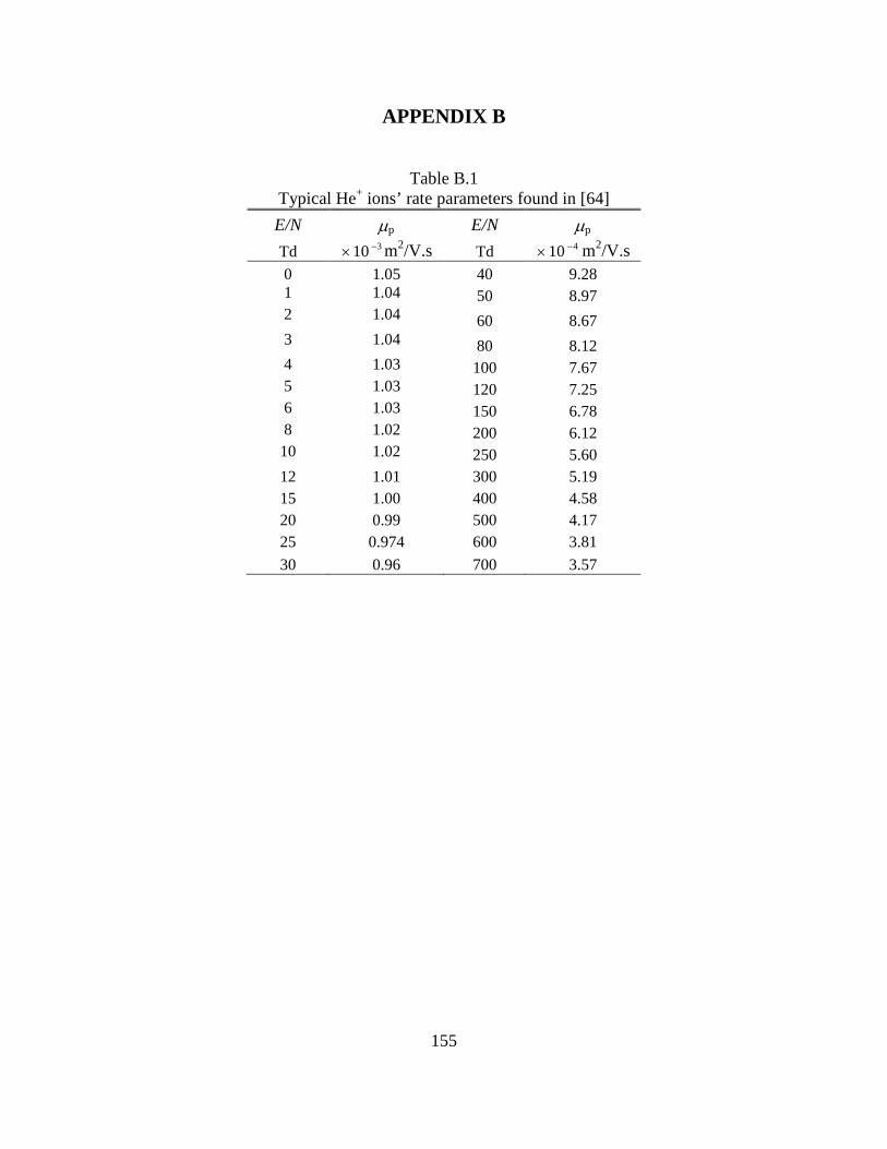
155
APPENDIX B
Table B.1 Typical He+ ions’ rate parameters found in [64]
E/N µp E/N µp
Td 310−× m2/V.s Td 410−× m2/V.s
0 1.05 40 9.28 1 1.04 50 8.97 2 1.04 60 8.67 3 1.04 80 8.12 4 1.03 100 7.67 5 1.03 120 7.25 6 1.03 150 6.78 8 1.02 200 6.12 10 1.02 250 5.60 12 1.01 300 5.19 15 1.00 400 4.58 20 0.99 500 4.17 25 0.974 600 3.81 30 0.96 700 3.57

156
APPENDIX C
Initial distribution of plasma parameters for 2D advective transport of plasma
Figure C.1. Area of the finite volumes
Figure C.2. Initial distribution of x-component of electric field

157
Figure C.3. Initial distribution of y-component of electric field
Figure C.4. Initial distribution of electrons mobility
Figure C.5. Initial distribution of positive ions mobility

158
Figure C.6. Initial distribution of electrons diffusion coefficient
Figure C.7. Initial distribution of electrons kinetic energy
Figure C.8. Initial distribution of ionization coefficient

159
Figure C.9. Initial distribution of generation term
Figure C.10. Initial distribution of x-component of electrons drift velocity
Figure C.11. Initial distribution of y-component of electrons drift velocity

160
Figure C.12. Initial distribution of x-component of positive ions drift velocity
Figure C.13. Initial distribution of y-component of positive ions drift velocity