High Performance Computing With Spatial Datasetsshekhar/talk/hpgis/10.11.acmgis.hpdgis.pdf · High...

1

High Performance Computing With

Spatial Datasets

Shashi ShekharMcKnight Distinguished University Professor

Department of Computer Science and Engineering

University of Minnesota

www.cs.umn.edu/~shekhar

2

Acknowledgments

• HPC Resources, Research Grants

– Army High Performance Computing Research Center-AHPCRC

– Minnesota Supercomputing Institute - MSI

• Spatial Database Group Members

– Mete Celik, Sanjay Chawla, Vijay Gandhi, Betsy George, James Kang,

Baris M. Kazar, QingSong Lu, Sangho Kim, Sivakumar Ravada

• USDOD

– Douglas Chubb, Greg Turner, Dale Shires, Jim Shine, Jim Rodgers

– Richard Welsh (NCS, AHPCRC), Greg Smith

• Academic Colleagues

– Vipin Kumar

– Kelley Pace, James LeSage

– Junchang Ju, Eric D. Kolaczyk, Sucharita Gopal

3

Overview

• Motivation for HPC with Spatial Data

– Ex. Application: Disaster Relief, Evacuation Planning

– Ex. Application: Geo-spatial Intelligence

• Case Study 1: Simple to Parallelize

• Case Study 2 – Harder

• Case Study 3 – Hardest

• Wrap-up

4

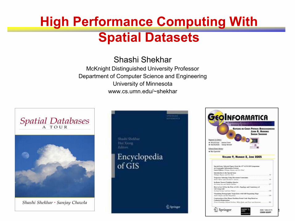
Example Application : Situation Assessment

• Where are the affected people?

• Which roads are navigable?

• Where may relief supplies to air-dropped?

• Where should distribution centers be located?

• What is the environment? What is the impact?

5

Example Application: Evacuation Planning

Lack of effective evacuation plans

Traffic congestions on all highways

Great confusions and chaos

"We packed up Morgan City residents to evacuate in the a.m. on the day that Andrew hit coastal Louisiana, but in early afternoon the majority came back home. The traffic was so bad that they couldn't get through Lafayette." Mayor Tim Mott, Morgan City, Louisiana ( http://i49south.com/hurricane.htm )

( FEMA.gov)

Hurricane Rita

evacueesfrom Houston

clog I-45.

( www.washingtonpost.com)

Hurricane Andrew

Florida and Louisiana, 1992

Hurricane Rita

Gulf Coast, 2005

( National Weather Services)

( National Weather Services)

6

Homeland Defense & Evacuation Planning

Preparation of response to a chem-bio attack

Plan evacuation routes and schedules

Help public officials to make important decisions

Guide affected population to safety

Base Map Weather Data

Plume

Dispersion

Demographics

Information

Transportation

Networks

( Images from www.fortune.com )

7

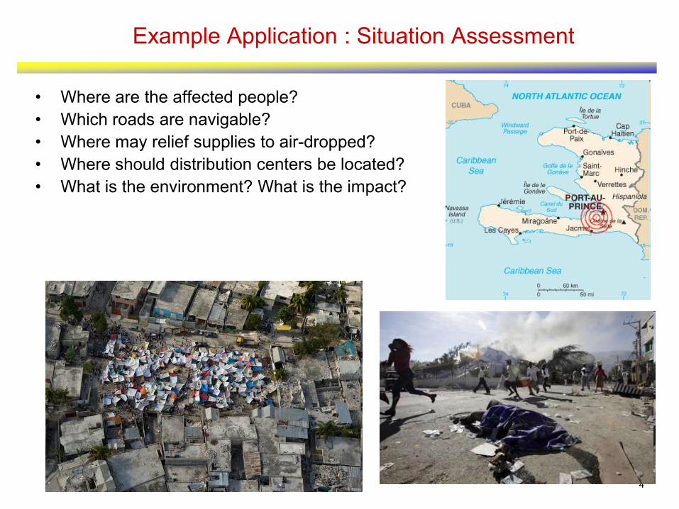
A Real Scenario

Nuclear Power Plants in Minnesota

Twin Cities

8

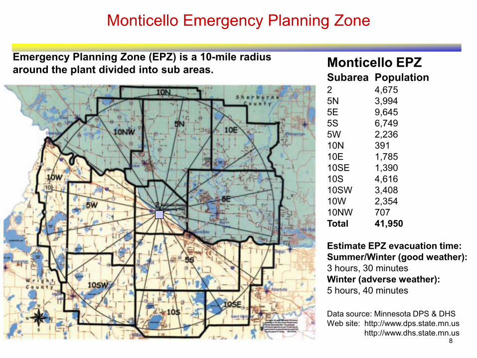
Monticello Emergency Planning Zone

Monticello EPZSubarea Population2 4,675

5N 3,994

5E 9,645

5S 6,749

5W 2,236

10N 391

10E 1,785

10SE 1,390

10S 4,616

10SW 3,408

10W 2,354

10NW 707

Total 41,950

Estimate EPZ evacuation time:

Summer/Winter (good weather):

3 hours, 30 minutes

Winter (adverse weather):

5 hours, 40 minutes

Emergency Planning Zone (EPZ) is a 10-mile radius

around the plant divided into sub areas.

Data source: Minnesota DPS & DHS

Web site: http://www.dps.state.mn.us

http://www.dhs.state.mn.us

9

Source cities

Destination

Monticello Power Plant

Routes used only by old plan

Routes used only by result plan of

capacity constrained routing

Routes used by both plans

Congestion is likely in old plan near evacuation

destination due to capacity constraints. Our plan

has richer routes near destination to reduce

congestion and total evacuation time.

A Real Scenario (Monticello): Result Routes

10

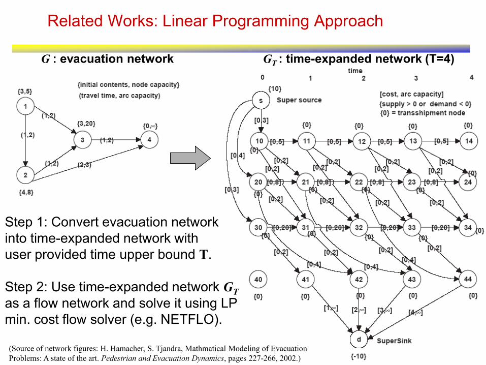
Related Works: Linear Programming Approach

Step 1: Convert evacuation network

into time-expanded network with

user provided time upper bound T.

G : evacuation network

Step 2: Use time-expanded network GT

as a flow network and solve it using LP

min. cost flow solver (e.g. NETFLO).

GT : time-expanded network (T=4)

(Source of network figures: H. Hamacher, S. Tjandra, Mathmatical Modeling of Evacuation

Problems: A state of the art. Pedestrian and Evacuation Dynamics, pages 227-266, 2002.)

11

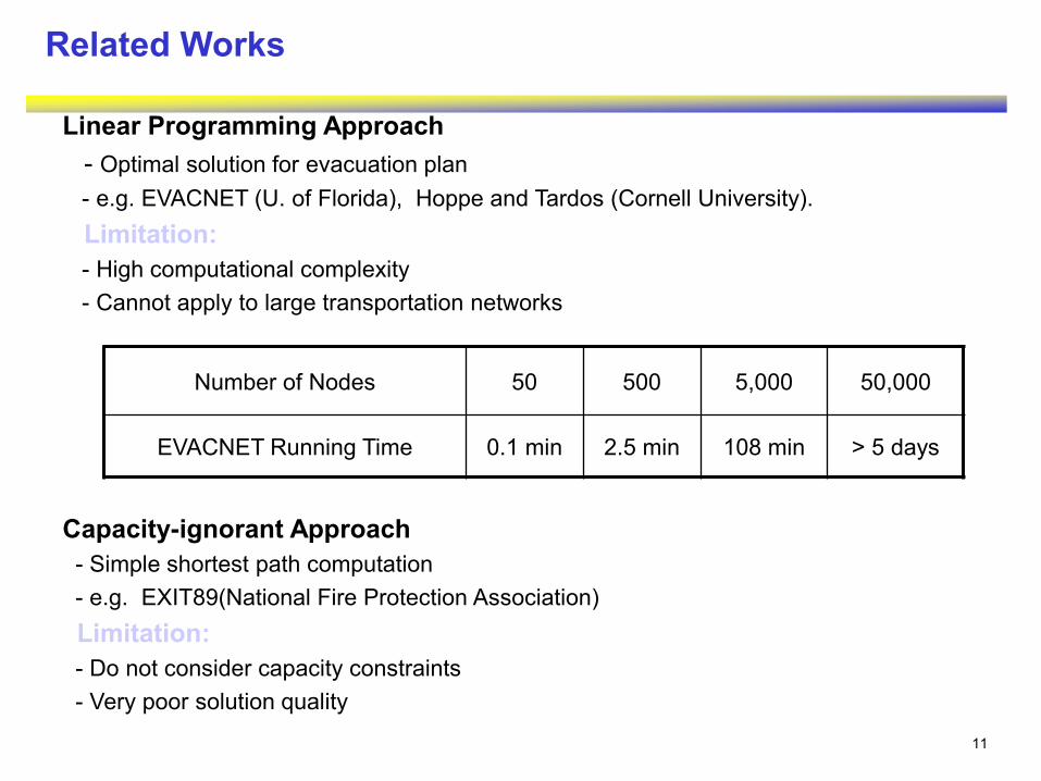
Linear Programming Approach

- Optimal solution for evacuation plan

- e.g. EVACNET (U. of Florida), Hoppe and Tardos (Cornell University).

Limitation:

- High computational complexity

- Cannot apply to large transportation networks

Capacity-ignorant Approach

- Simple shortest path computation

- e.g. EXIT89(National Fire Protection Association)

Limitation:

- Do not consider capacity constraints

- Very poor solution quality

Number of Nodes 50 500 5,000 50,000

EVACNET Running Time 0.1 min 2.5 min 108 min > 5 days

Related Works

12

Overview



– Multi-Scale Multi-Granular Classification

– Motivation, Problem Definition

– Serial Version

– Alternative parallelization

– Evaluation



• Wrap-up

13

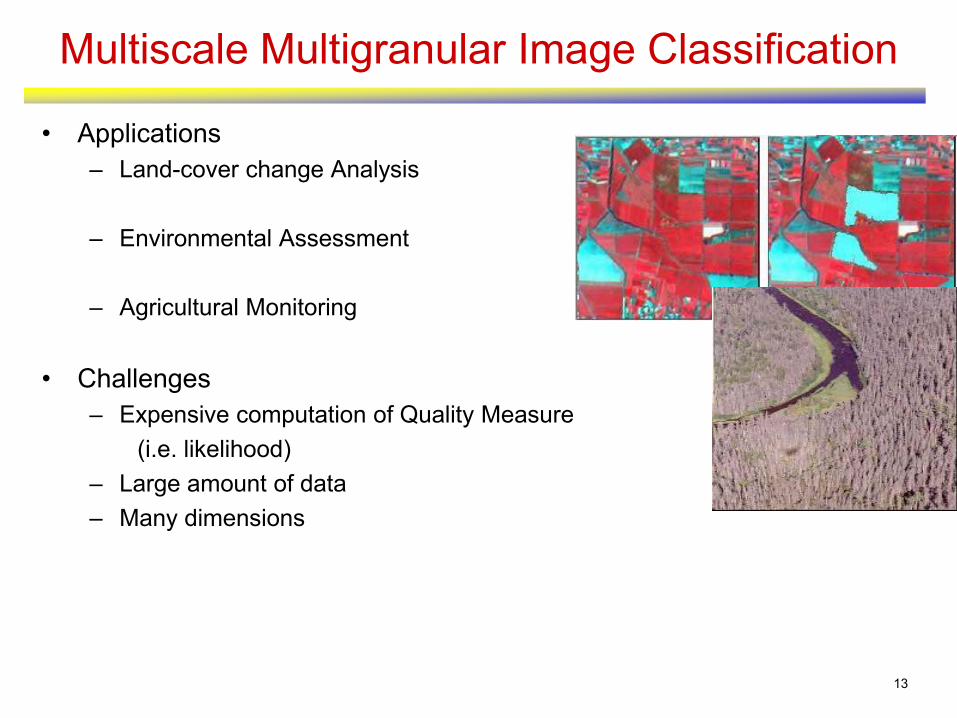
Multiscale Multigranular Image Classification

• Applications

– Land-cover change Analysis

– Environmental Assessment

– Agricultural Monitoring

• Challenges

– Expensive computation of Quality Measure

(i.e. likelihood)

– Large amount of data

– Many dimensions

14

Spatial Applications: An Example

• Multiscale Multigranular Image Classification

Inputs

Output Images at

Multiple Scales

15

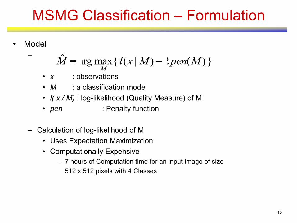
MSMG Classification – Formulation

• Model

–

• x : observations

• M : a classification model

• l( x / M) : log-likelihood (Quality Measure) of M

• pen : Penalty function

– Calculation of log-likelihood of M

• Uses Expectation Maximization

• Computationally Expensive

– 7 hours of Computation time for an input image of size

512 x 512 pixels with 4 Classes

})(2)|({maxargˆ MpenMxlMM

16

Pseudo-code : Serial Version

1. Initialize parameters.

2. for each Class

3. for each Spatial Scale

4. for each Quad

5. Calculate Quality Measure (i.e., log-likelihood)

8. end for Quad

9. end for Spatial Scale

10. end for Class

11. Post-processing

Q? What are the options for parallelization?

17

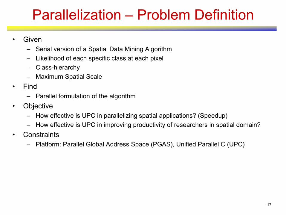
Parallelization – Problem Definition

• Given

– Serial version of a Spatial Data Mining Algorithm

– Likelihood of each specific class at each pixel

– Class-hierarchy

– Maximum Spatial Scale

• Find

– Parallel formulation of the algorithm

• Objective

– How effective is UPC in parallelizing spatial applications? (Speedup)

– How effective is UPC in improving productivity of researchers in spatial domain?

• Constraints

– Platform: Parallel Global Address Space (PGAS), Unified Parallel C (UPC)

18

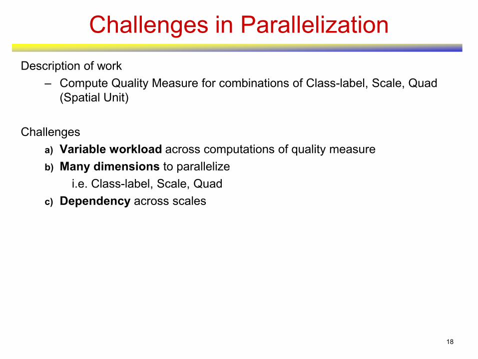
Challenges in Parallelization

Description of work

– Compute Quality Measure for combinations of Class-label, Scale, Quad

(Spatial Unit)

Challenges

a) Variable workload across computations of quality measure

b) Many dimensions to parallelize

i.e. Class-label, Scale, Quad

c) Dependency across scales

19

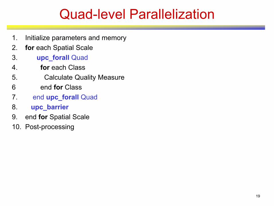
Quad-level Parallelization

1. Initialize parameters and memory

2. for each Spatial Scale

3. upc_forall Quad

4. for each Class

5. Calculate Quality Measure

6 end for Class

7. end upc_forall Quad

8. upc_barrier

9. end for Spatial Scale

10. Post-processing

20

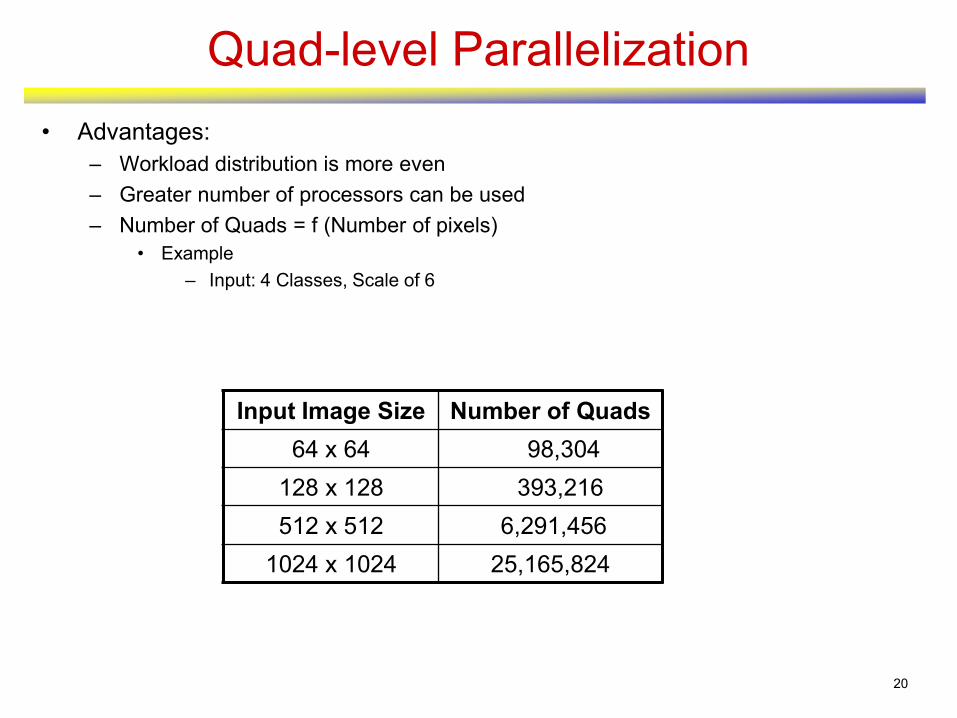
Quad-level Parallelization

• Advantages:

– Workload distribution is more even

– Greater number of processors can be used

– Number of Quads = f (Number of pixels)

• Example

– Input: 4 Classes, Scale of 6

Input Image Size Number of Quads

64 x 64 98,304

128 x 128 393,216

512 x 512 6,291,456

1024 x 1024 25,165,824

21

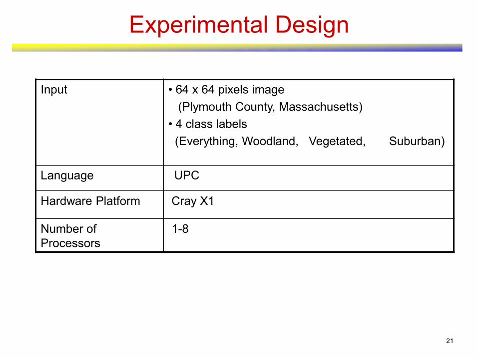
Experimental Design

Input • 64 x 64 pixels image

(Plymouth County, Massachusetts)

• 4 class labels

(Everything, Woodland, Vegetated, Suburban)

Language UPC

Hardware Platform Cray X1

Number of

Processors

1-8

22

Workload

Input class hierarchy

Scale: 64 x 64 Scale: 2 x 2

Output Images at Multiple scales

23

Effect of Number of Processors

• Quad-level parallelization gives better speed-up

• Room for Speed-up for both approaches

• Q? Class-level << Quad-level. Why?

0

0.25

0.5

0.75

1

1 2 4 8

Number of Processors

Eff

icie

nc

y

Class-level

Quad-level0

1

2

3

4

5

6

7

2 4 8Number of Processors

Sp

ee

du

p

Class-level

Quad-level

24

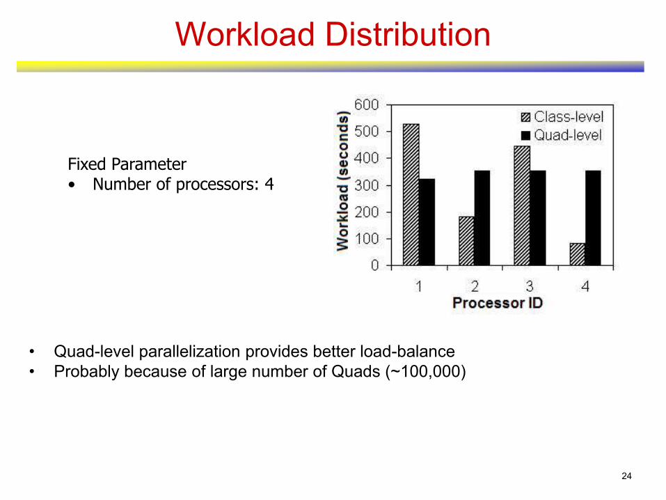
Workload Distribution

• Quad-level parallelization provides better load-balance

• Probably because of large number of Quads (~100,000)

Fixed Parameter • Number of processors: 4

25

Findings - I

• How effective is UPC in parallelizing Spatial applications?

– Quad-level parallelization

• Speed-up of 6.65 on 8 processors

• Large number of Quads (98,304)

– Class-level parallelization

• Speed-ups are lower

• Smaller number of Classes (4)

26

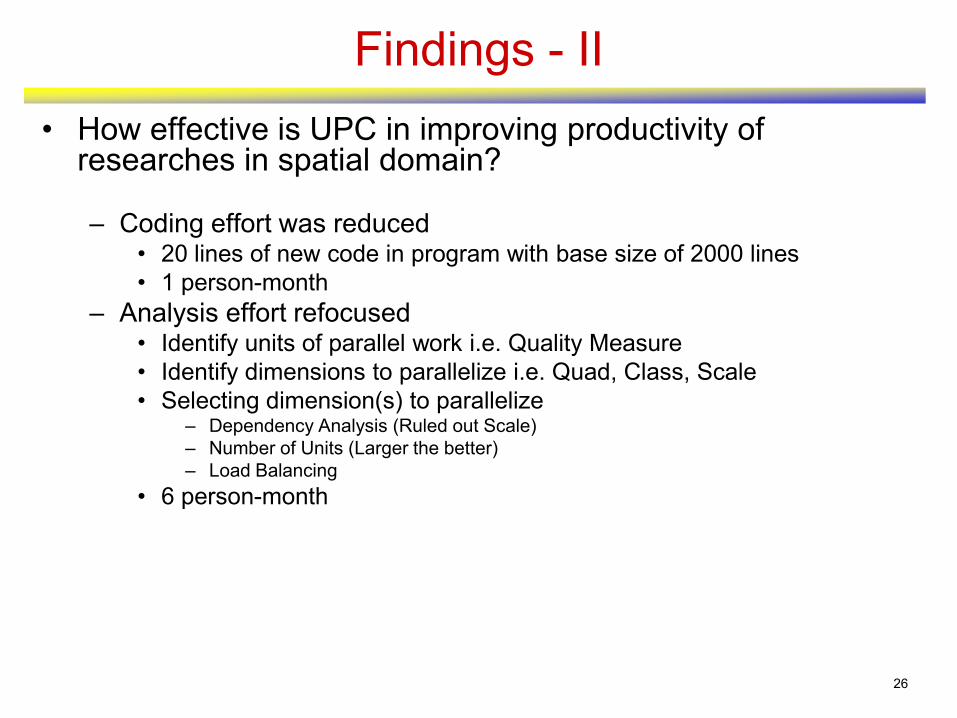
Findings - II

• How effective is UPC in improving productivity of researches in spatial domain?

– Coding effort was reduced• 20 lines of new code in program with base size of 2000 lines

• 1 person-month

– Analysis effort refocused• Identify units of parallel work i.e. Quality Measure

• Identify dimensions to parallelize i.e. Quad, Class, Scale

• Selecting dimension(s) to parallelize– Dependency Analysis (Ruled out Scale)

– Number of Units (Larger the better)

– Load Balancing

• 6 person-month

27

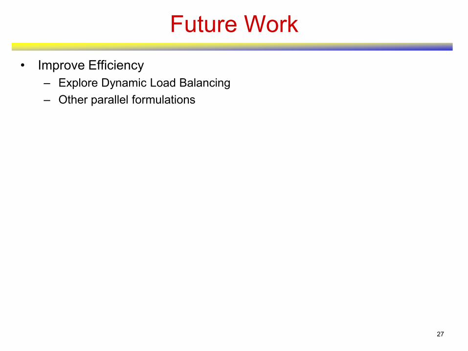
Future Work

• Improve Efficiency

– Explore Dynamic Load Balancing

– Other parallel formulations

28

Overview




– Spatial Databases: Parallelizing Range Query

– Basic Concepts & Problem Formulation

– Declustering Spatial Data

– Dynamic Load Balancing (DLB) for Spatial Data


• Wrap-up

29

Range Query - Motivation

• GIS Based Augmented/Virtual Reality

– GIS fetches polygons (feature-data plus elevation-data)

– Transform polygons to 3-D objects (e.g. trees, buildings, etc.)

– Render 3-D objects

• Other Applications

– RealTime Terrain Visualization

– Interactive Situation Assessment

– Interactive Spatial Decision Making, etc.

30

Range Query Motivation - 2

• High Performance Requirements (mid-1990s)

– limit on response time: < 1/2 sec

– latest processors can process < 1500 polygons in 1/2 sec

– typical requirement: process more than 10,000 polygons

• An Example Map

• Q?. Are Sequential Approaches Adequate?

• Q?. Can Parallel Solutions Meet the Requirements?

31

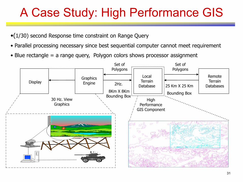
A Case Study: High Performance GIS

•(1/30) second Response time constraint on Range Query

• Parallel processing necessary since best sequential computer cannot meet requirement

• Blue rectangle = a range query, Polygon colors shows processor assignment

Set of Polygons

Set of Polygons

DisplayGraphics Engine

Local Terrain

Database

Remote Terrain

Databases

30 Hz. View Graphics

2Hz.

8Km X 8Km Bounding Box

High Performance

GIS Component

25 Km X 25 Km

Bounding Box

32

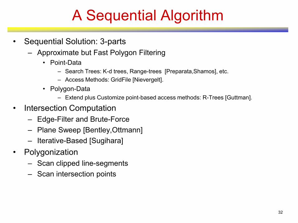
A Sequential Algorithm

• Sequential Solution: 3-parts

– Approximate but Fast Polygon Filtering

• Point-Data

– Search Trees: K-d trees, Range-trees [Preparata,Shamos], etc.

– Access Methods: GridFile [Nievergelt].

• Polygon-Data

– Extend plus Customize point-based access methods: R-Trees [Guttman].

• Intersection Computation

– Edge-Filter and Brute-Force

– Plane Sweep [Bentley,Ottmann]

– Iterative-Based [Sugihara]

• Polygonization

– Scan clipped line-segments

– Scan intersection points

33

Approximate but Fast Polygon Filtering

• Grid-Directory

• Each grid cell contains the list of polygons intersecting the cell

• Indices on both x and y axis

34

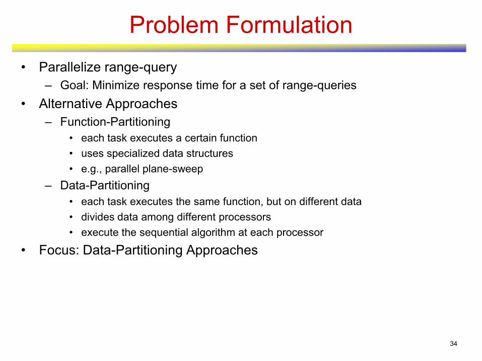
Problem Formulation

• Parallelize range-query

– Goal: Minimize response time for a set of range-queries

• Alternative Approaches

– Function-Partitioning

• each task executes a certain function

• uses specialized data structures

• e.g., parallel plane-sweep

– Data-Partitioning

• each task executes the same function, but on different data

• divides data among different processors

• execute the sequential algorithm at each processor

• Focus: Data-Partitioning Approaches

35

Issues in Data-Partitioning

• Partitioning the data

– partition polygons at different levels

• edges, sub-polygons, polygons

– partition range-query

• smaller range-queries, edges

• Focus

– partition data at polygon level

– Range-query is not partitioned

36

Data-Partitioning Approach

• Initial Static Partitioning

• Run-Time dynamic load-balancing (DLB)

37

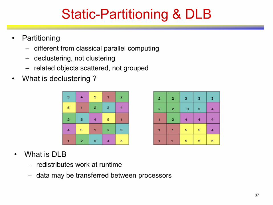
Static-Partitioning & DLB

• Partitioning

– different from classical parallel computing

– declustering, not clustering

– related objects scattered, not grouped

• What is declustering ?

• What is DLB

– redistributes work at runtime

– data may be transferred between processors

38

Scope of this Work

• No pre-computation except index

• Main-Memory database

• Each range-query is independent

• Data-partitioning, not function-partitioning

• Granularity of partition is polygon

39

Declustering Polygonal Maps

Example:

• Dividing a Map among 4 processors.

• Polygons within a processor have common color

• Green rectangle = a range query

Goals of declustering

• balance load acrosss proessors

• for arbitrary range query

Challenges

• Large polygons – upper right

• Variation in polygon sizes

40

Declustering Spatial Data

• Goal of Declustering

– partition the data so that each partition imposes exactly the same load for any range-query

• Theorem: Declustering is NP-hard

• Definition: Declustering Problem

– Given:

• Set S of extended-objects

• P processors

• Set Q = (Q1 …. Qn) of n range-queries

– Partition the set S among P processors

– Such that:

• load at each processor is balanced for all Qi Є Q

– Where load of an object x Є S for a given range-query Qi is given by

• fQi : Z

• Z is the set of nonnegative integers

42

Issues in Declustering Polygonal Maps

• Declustering method

• Work-Load metric

• Spatial-Extent of workload

• Distribution of the workload over spatial-extent

43

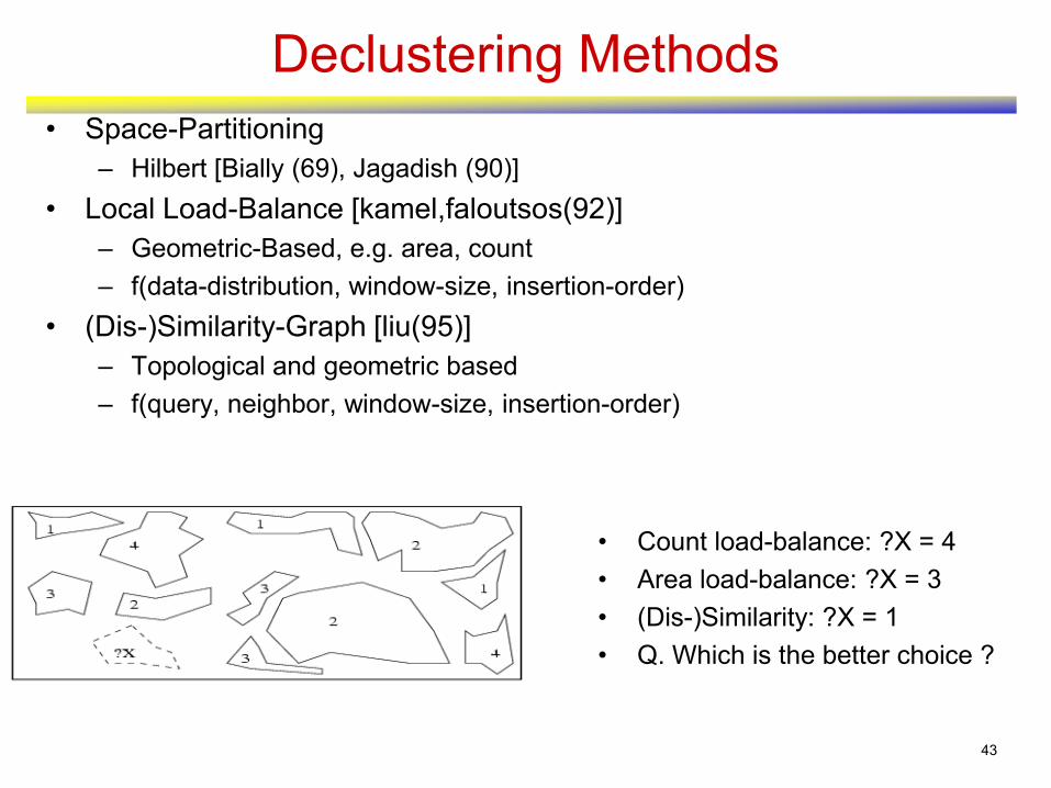
Declustering Methods

• Space-Partitioning

– Hilbert [Bially (69), Jagadish (90)]

• Local Load-Balance [kamel,faloutsos(92)]

– Geometric-Based, e.g. area, count

– f(data-distribution, window-size, insertion-order)

• (Dis-)Similarity-Graph [liu(95)]

– Topological and geometric based

– f(query, neighbor, window-size, insertion-order)

• Count load-balance: ?X = 4

• Area load-balance: ?X = 3

• (Dis-)Similarity: ?X = 1

• Q. Which is the better choice ?

47

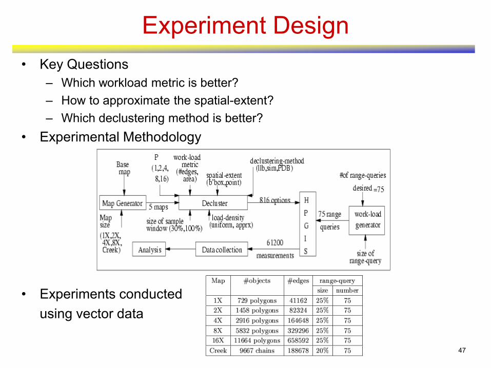
Experiment Design

• Key Questions

– Which workload metric is better?

– How to approximate the spatial-extent?

– Which declustering method is better?

• Experimental Methodology

• Experiments conducted

using vector data

48

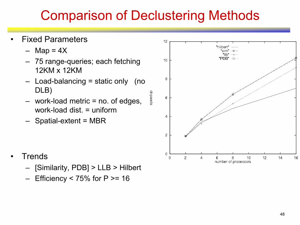
Comparison of Declustering Methods

• Fixed Parameters

– Map = 4X

– 75 range-queries; each fetching

12KM x 12KM

– Load-balancing = static only (no

DLB)

– work-load metric = no. of edges,

work-load dist. = uniform

– Spatial-extent = MBR

• Trends

– [Similarity, PDB] > LLB > Hilbert

– Efficiency < 75% for P >= 16

49

Comparison of Declustering Methods


– Map = Creek

– 75 range-queries; each fetching

12KM x 12KM

– Load-balancing = static only (no

DLB)

– work-load metric = no. of edges,

work-load dist. = uniform

– Spatial-extent = MBR

• Trends

– [Similarity, PDB] > LLB > Hilbert

– Efficiency < 75% for P >= 16

50

Effect of Range-Query Size


• Map = 4X

• Load-balancing = static only (no DLB)

• workload metric = no. of edges, workload dist. = uniform

• Spatial-extent = MBR

51

Dynamic Load-Balancing (DLB)

• DLB is used if static declustering methods fail to balance the load

• Issues in DLB

– Methods for transferring work

– Partitioning method & Granularity of work transfers

– Which processor should an idle processor ask for more work?

52

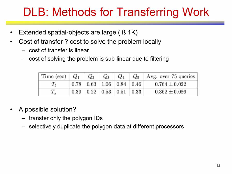
DLB: Methods for Transferring Work

• Extended spatial-objects are large ( ß 1K)

• Cost of transfer ? cost to solve the problem locally

– cost of transfer is linear

– cost of solving the problem is sub-linear due to filtering

• A possible solution?

– transfer only the polygon IDs

– selectively duplicate the polygon data at different processors

55

Pool-Size Choice is Challenging!

56

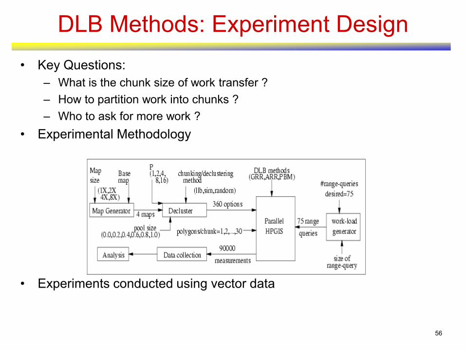
DLB Methods: Experiment Design

• Key Questions:

– What is the chunk size of work transfer ?

– How to partition work into chunks ?

– Who to ask for more work ?

• Experimental Methodology

• Experiments conducted using vector data

57

DLB: Experiment Design

• Hardware

– CrayT3D (mid-1990s)

• Distributed memory with fast interconnection network

• Each node is a DEC-Alpha (150MHz)

– SGI Challenge

• Shared-Memory with fast bus

• Each node is a MIPS 4400 (200MHz)

• Software

– Sequential code (8K lines) plus communication routines

– C processes with partial shared address space

– Shared-Memory library (both T3D and SGI)

59

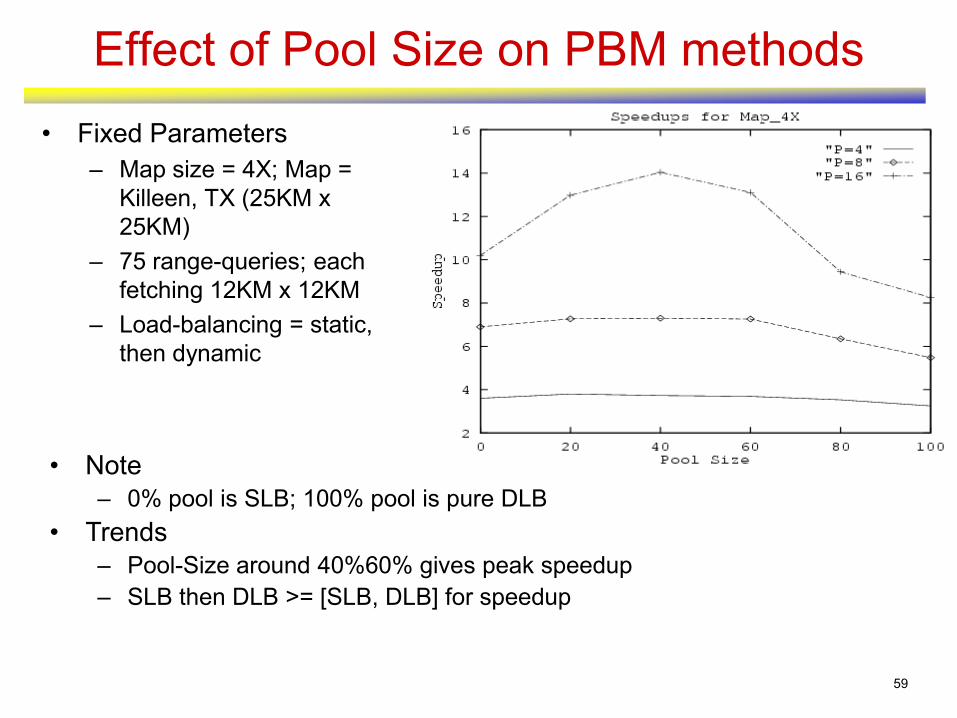
Effect of Pool Size on PBM methods


– Map size = 4X; Map =

Killeen, TX (25KM x

25KM)

– 75 range-queries; each

fetching 12KM x 12KM

– Load-balancing = static,

then dynamic

• Note

– 0% pool is SLB; 100% pool is pure DLB

• Trends

– Pool-Size around 40%60% gives peak speedup

– SLB then DLB >= [SLB, DLB] for speedup

60

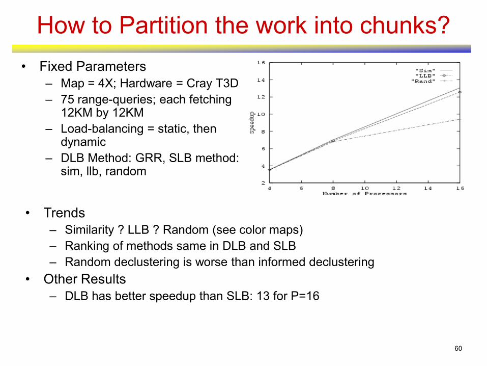
How to Partition the work into chunks?


– Map = 4X; Hardware = Cray T3D

– 75 range-queries; each fetching 12KM by 12KM

– Load-balancing = static, then dynamic

– DLB Method: GRR, SLB method: sim, llb, random

• Trends

– Similarity ? LLB ? Random (see color maps)

– Ranking of methods same in DLB and SLB

– Random declustering is worse than informed declustering

• Other Results

– DLB has better speedup than SLB: 13 for P=16

61

Research Contributions

• Static Load-Balancing - Declustering Spatial Data

– proposed new declustering methods outperform traditional methods

– neither static declustering nor DLB alone are sufficient to provide good

speedups

– declustering can be used to improve the performance of DLB

• Dynamic Load-Balancing (DLB)

– How to manage work transfers?

• selectively duplicate the polygons at different processors

• transfer the polygon Ids

– How to partition the work?

• Chunks-cheduling is interesting for spatial data

• declustering can be used to partition the work into chunks

– DistributedMemory vs SharedMemory

• Able to solve bigger maps on sharedmemory machine

• Declustering is interesting for both the architectures

62

Overview





– Spatial Data Mining: Parallelizing Spatial Auto-regression

• Key Concepts & Problem Definition

• Parallel Spatial Auto-Regression

• Experimental Results

• Wrap-up

63

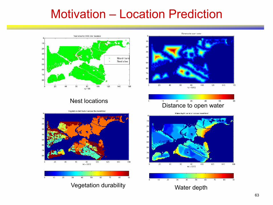
Motivation – Location Prediction

Nest locationsDistance to open water

Vegetation durability Water depth

64

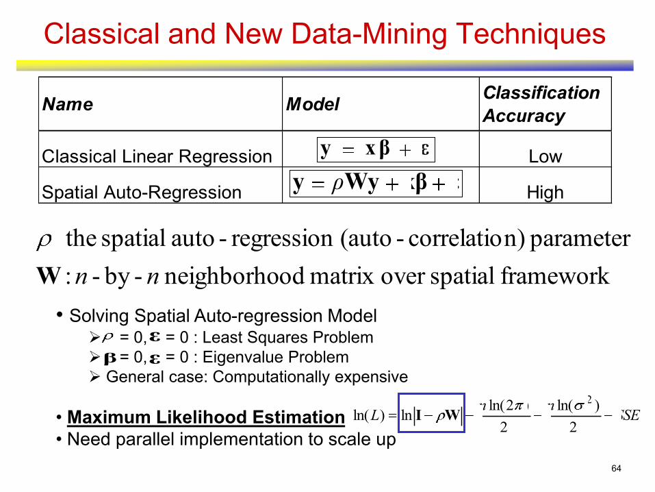
Classical and New Data-Mining Techniques

Classical Linear Regression Low

Spatial Auto-Regression High

Name ModelClassification

Accuracy

εxβy

εxβWyy ρ

framework spatialover matrix odneighborho -by- :

parameter n)correlatio-(auto regression-auto spatial the:

nnW

• Solving Spatial Auto-regression Model = 0, = 0 : Least Squares Problem

= 0, = 0 : Eigenvalue Problem

General case: Computationally expensive

• Maximum Likelihood Estimation

• Need parallel implementation to scale up

β

ε

ε

SSEnn

L2

)ln(

2

)2ln(ln)ln(

2

WI

65

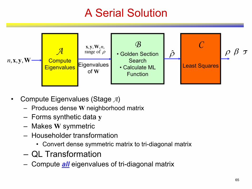
A Serial Solution

B• Golden Section

Search

• Calculate ML

Function

ACompute

Eigenvalues

C

Least SquaresEigenvalues

of W

of range,,,, nWyx

2

ˆ,ˆ,ˆˆWyx ,,,n

• Compute Eigenvalues (Stage A)

– Produces dense W neighborhood matrix

– Forms synthetic data y

– Makes W symmetric

– Householder transformation

• Convert dense symmetric matrix to tri-diagonal matrix

– QL Transformation– Compute all eigenvalues of tri-diagonal matrix

66

Serial Response Times (sec)

• Stage A is the bottleneck & Stage B and C contribute very small to response time

0

1000

2000

3000

4000

5000

6000

7000

SGI

Origin

IBM SP IBM

Regatta

SGI

Origin

IBM SP IBM

Regatta

SGI

Origin

IBM SP IBM

Regatta

2500 6400 10000

Problem Sizes on Different Machines

Tim

e (

se

c)

Stage A Stage B Stage C

68

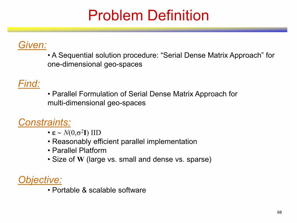
Problem Definition

Given:• A Sequential solution procedure: “Serial Dense Matrix Approach” for

one-dimensional geo-spaces

Find:• Parallel Formulation of Serial Dense Matrix Approach for

multi-dimensional geo-spaces

Constraints:• N(0, 2I) IID

• Reasonably efficient parallel implementation

• Parallel Platform

• Size of W (large vs. small and dense vs. sparse)

Objective:• Portable & scalable software

69

Related Work & Our Contributions

• Related work: Li, 1996

– Limitations: Solved 1-D problem

• Our Contributions

– Parallel solution for 2-D problems

– Portable software

• Fortran 77

• An Application of Hybrid Parallelism

• MPI messaging system

• Compiler directives of OpenMP

70

Our Approach – Parallel Spatial Auto-Regression

• Function vs. Data Partitioning

– Function partitioning: Each processor works on the same data with different instructions

– Data partitioning (applied): Each processor works on different data with the same instructions

• Implementation Platform:

– Produces dense W neighborhood matrix

– Fortran with MPI & OpenMP API’s

• No machine-specific compiler directives

– Portability

– Help software development and technology transfer

• Other Performance Tuning

– Static terms computed once

71

02

1002

100000000000

310

3100

310000000000

03

103

1003

1000000000

002

100002

100000000

310000

3100

310000000

04

1004

104

1004

1000000

004

1004

104

1004

100000

0003

1003

100003

10000

00003

100003

1003

1000

000004

1004

104

1004

100

0000004

1004

104

1004

10

00000003

1003

100003

1

000000002

100002

100

0000000003

1003

103

10

00000000003

1003

103

1

000000000002

1002

10

Contiguous16 15 14 13 12 11 10 9 8 7 6 5 4 3 2 1

P1 P1 P1 P1P2 P2 P2 P2

P3 P3 P3 P3P4 P4 P4 P4

02

1002

100000000000

310

3100

310000000000

03

103

1003

1000000000

002

100002

100000000

310000

3100

310000000

04

1004

104

1004

1000000

004

1004

104

1004

100000

0003

1003

100003

10000

00003

100003

1003

1000

000004

1004

104

1004

100

0000004

1004

104

1004

10

00000003

1003

100003

1

000000002

100002

100

0000000003

1003

103

10

00000000003

1003

103

1

000000000002

1002

10

P1

P2

P3

P4

P1

P2

P3

P4

P1

P2

P3

P4

P1

P2

P3

P4

Round-robin with chunk size 116 15 14 13 12 11 10 9 8 7 6 5 4 3 2 1

Data Partitioning in a Smaller Scale

• 4 processors are used and

chunk size can be determined by the user

• W is 16-by-16 and partitioned across processors

P1- (40 vs. 58)

P2- (36 vs. 42)

P3- (32 vs. 26)

P4- (28 vs. 10)

72

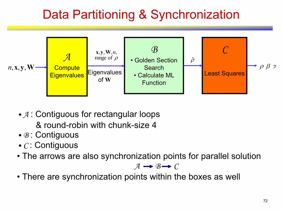
• A : Contiguous for rectangular loops

& round-robin with chunk-size 4 • B : Contiguous

• C : Contiguous

• The arrows are also synchronization points for parallel solutionA B C

• There are synchronization points within the boxes as well

Data Partitioning & Synchronization

B• Golden Section

Search

• Calculate ML

Function

ACompute

Eigenvalues

C

Least SquaresEigenvalues

of W

of range,,,, nWyx

2ˆ,ˆ,ˆˆ

Wyx ,,,n

73

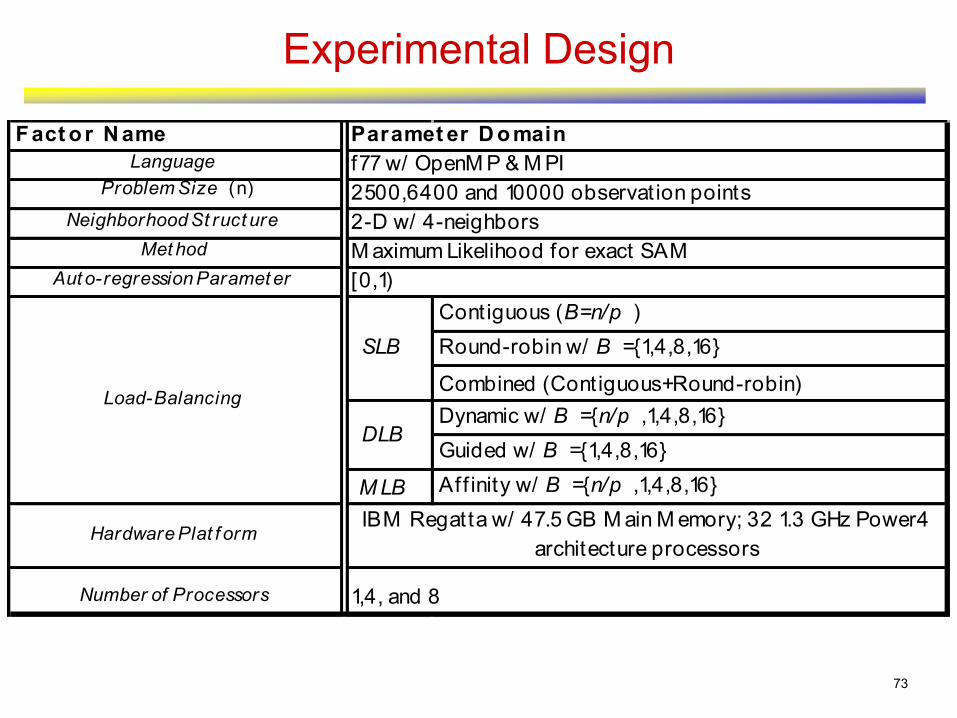
Experimental Design

Fact o r N ame

Language

Problem Size (n)

Neighborhood St ruct ure

Met hod

Aut o-regression Paramet er

Contiguous (B=n/p )

Round-robin w/ B ={1,4,8,16}

Combined (Contiguous+Round-robin)

Dynamic w/ B ={n/p ,1,4,8,16}

Guided w/ B ={1,4,8,16}

M LB Aff inity w/ B ={n/p ,1,4,8,16}

Number of Processors

M aximum Likelihood for exact SAM

[0,1)

SLB

DLB

Paramet er D omain

f77 w/ OpenM P & M PI

2500,6400 and 10000 observat ion points

2-D w/ 4-neighbors

IBM Regatta w/ 47.5 GB M ain M emory; 32 1.3 GHz Power4

architecture processorsHardware Plat f orm

1,4, and 8

Load-Balancing

74

Experimental Results – Effect of Load Balancing

Effect of Load-Balancing Techniques on Speedup

for Problem Size 10000

0

1

2

3

4

5

6

7

8

1 4 8Number of Processors

Sp

eed

up

mixed1 Static B=8 Dynamic B=8 Affinity B=1 Guided B=16

75

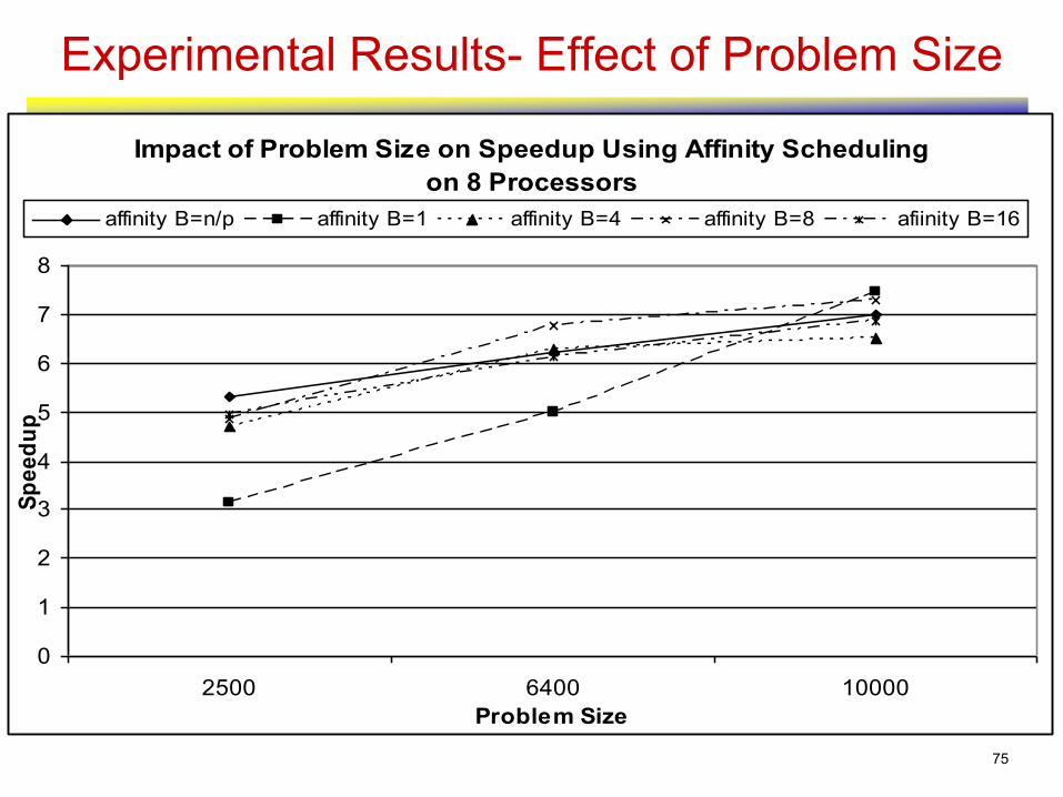
Experimental Results- Effect of Problem Size

Impact of Problem Size on Speedup Using Affinity Scheduling

on 8 Processors

0

1

2

3

4

5

6

7

8

2500 6400 10000

Problem Size

Sp

ee

du

p

affinity B=n/p affinity B=1 affinity B=4 affinity B=8 afiinity B=16

76

Parallel SAR - Summary

• Developed a parallel formulation of spatial auto-regression

model

• Estimates maximum likelihood of regular square tessellation 1-

D and 2-D planar surface partitionings for location prediction

problems

• Used dense eigenvalue computation and hybrid parallel

programming

77

Parallel SAR - Future Work

1. Understand reasons of inefficiencies

– Algebraic cost model for speedup measurements on different

architectures

2. Fine tune implemented parallel formulation

– Consider alternate parallel formulations

3. Parallelize other serial solutions using sparse-matrix techniques

− Chebyshev Polynomial approximation

− Markov Chain Monte Carlo Estimator

78

Overview





• Wrap-up

79

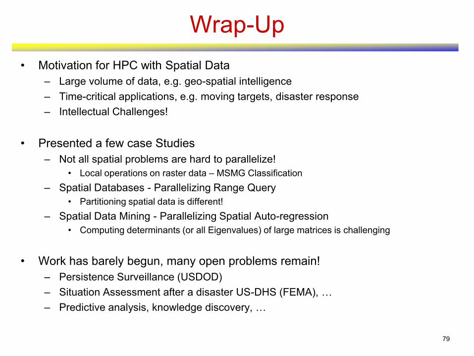
Wrap-Up


– Large volume of data, e.g. geo-spatial intelligence

– Time-critical applications, e.g. moving targets, disaster response

– Intellectual Challenges!

• Presented a few case Studies

– Not all spatial problems are hard to parallelize!

• Local operations on raster data – MSMG Classification

– Spatial Databases - Parallelizing Range Query

• Partitioning spatial data is different!

– Spatial Data Mining - Parallelizing Spatial Auto-regression

• Computing determinants (or all Eigenvalues) of large matrices is challenging

• Work has barely begun, many open problems remain!

– Persistence Surveillance (USDOD)

– Situation Assessment after a disaster US-DHS (FEMA), …

– Predictive analysis, knowledge discovery, …

High Performance Computing With Spatial Datasetsshekhar/talk/hpgis/10.11.acmgis.hpdgis.pdf · High...

Documents

Transcript of High Performance Computing With Spatial Datasetsshekhar/talk/hpgis/10.11.acmgis.hpdgis.pdf · High...