High performance computation of landscape genomicmodels integrating local indices of spatial association

Sylvie Stucki1, Pablo Orozco-terWengel2, Michael W. Bruford2, Licia Colli3,Charles Masembe4, Riccardo Negrini3,5, Pierre Taberlet5,6, Stéphane Joost1,∗ , and

the NEXTGEN Consortium8

1Laboratory of Geographic Information Systems (LASIG), School ofArchitecture, Civil and Environmental Engineering (ENAC), Ecole

Polytechnique Fédérale de Lausanne (EPFL), 1015 Lausanne, Switzerland2School of Biosciences, Sir Martin Evans Building, Cardiff University, Cardiff, UK3Istituto di Zootecnica and BioDNA - Centro di Ricerca sulla Biodiversità e sul

DNA Antico, Università Cattolica del S. Cuore, via E. Parmense 84, 29100Piacenza, Italy

4Makerere University, Institute of Environment and Natural Resources,Molecular Biology Laboratory, Kampala, Uganda

5Associazione Italiana Allevatori, Roma, Italy6CNRS, Laboratoire d’Ecologie Alpine, Grenoble, France

7Univ. Grenoble Alpes, Laboratoire d’Ecologie Alpine, Grenoble, France8http://nextgen.epfl.ch

February 3, 2022

Abstract

Motivation: The increasing availability of high-throughput datasets requires power-ful methods to support the detection of signatures of selection in landscape genomics.Results: We present an integrated approach to study signatures of local adaptation,providing rapid processing of whole genome data and enabling assessment of spatialassociation using molecular markers.Availabilty: Samβada is an open source software written in C++ available athttp:lasig.epfl.ch/sambada (under the license GNU GPL 3). Compiled versions areprovided for Windows, Linux and MacOS X.Contact: stephane.joost@epfl.ch, sylvie.stucki@a3.epfl.chSupplementary material is available online.

∗to whom correspondence should be addressed

1

arX

iv:1

405.

7658

v1 [

q-bi

o.PE

] 2

9 M

ay 2

014

1 IntroductionThe time interval between Mitton et al.’s (1977) first attempt to correlate allelic frequen-cies with environmental variables to look for signatures of selection in ponderosa pine,and Joost et al.’s (2007; 2008) application of this concept allowing parallel processingof large numbers of logistic regressions was otherwise marked by little developments.During this period correlative approaches were used in parallel with population geneticsoutlier-detection methods (e.g. Beaumont and Nichols, 1996; Vitalis et al., 2003; Foll andGaggiotti, 2008) as cross-validation (e.g. Jones et al., 2013; Henry and Russello, 2013)to detect signatures of selection (see a review in Vitti et al., 2013). However, while suchmethods are still in vogue (e.g. Colli et al., 2014), there has been a revival in the interestof developing new statistical approaches for the emerging field of landscape genomics(e.g. Coop et al., 2010; Günther and Coop, 2013; Frichot et al., 2013; Guillot et al.,2014). For example, BayEnv (Günther and Coop, 2013) implements a Bayesian methodto compute correlations between allele frequencies and ecological variables taking intoaccount differences in sample sizes and shared demographic history. LFMM (Frichotet al., 2013) estimates the influence of population structure on allele frequencies by in-troducing unobserved variables as latent factors. Finally, SGLMM (Guillot et al., 2014)uses a spatially-explicit computational framework including a random effect to quantifythe correlation between genotypes and environmental variables. Yet, important func-tions are still lacking such as high performance computing capacity to process wholegenome data, and the integration of spatial statistics to support a distinction betweenselection and demographic signals. Here we present the software Samβada, which aimsat filling these gaps offering an open source multivariate analysis framework to detectsignatures of selection. Samβada’s use is illustrated with a case study dedicated to thedetection of potentially adaptive loci in 813 Bos taurus and Bos indicus individuals inUganda genotyped for ∼ 40,000 SNP. Lastly, Samβada’s performance is described withrespect to other state of the art software to detect signatures of selection.

2 Methods2.1 Samβada’s approachSamβada uses logistic regressions to model the probability of presence of an allelic variantfor a polymorphic marker given the environmental conditions of the sampling locations(Joost et al., 2007). Since each of the states of a given character is considered indepen-dently (i.e. as binary presence/absence in each sample), Samβadacan handle many typesof molecular data (e.g. SNPs, indels, copy number variants and haplotypes), providedthe user formats the input. Specifically, biallelic SNPs are recoded as three distinct geno-types. A maximum likelihood approach is used to fit the models (Dobson and Barnett,2008).

2

2.1.1 Univariate analysis

In the univariate case, each model for a given genotype is compared to a constantmodel, where the probability of presence is the same at each location and is equal to thefrequency of the genotype. Significance is assessed with both log-likelihood ratio (G) andWald tests (Dobson and Barnett, 2008). Bonferroni correction is applied for multiplecomparisons. In order to avoid numerous computations of p-values, the significancethreshold α is converted to a minimum score threshold. G and Wald scores are usedto compare models rather than Akaike or Bayesian information criterion in order toautomate model selection.

2.2 Multivariate analysisThe model selection procedure is adapted to assess the significance of multivariate mod-els. Both G and Wald tests refer to a null model to build the null hypothesis. Thecurrent model can be compared to the constant model (the same as in the univariateanalysis) using multivariate χ2 statistics. While rejecting the null hypothesis in thisconfiguration indicates that at least one parameter is statistically significant, it doesnot provide information about which parameter(s) is relevant to the model. Thereforemodel selection is based on simpler models nested in the current one, and parametersignificance is determined with either a Wald test applied to each parameter separately(except the constant parameter) or with G tests excluding a parameter at the time. Forthe latter, if a model A has q parameters, we define the parents of A as the q modelswith q − 1 parameters obtained by dropping one parameter from A. For instance, if Amodels the occurrence of genotype Xi with 3 environmental variables E2, E3 and E5,

A = (Xi|E2, E3, E5),

then the parents of A are the three models

(Xi|E2, E3), (Xi|E2, E5) and (Xi|E3, E5).

The parent of A with the highest log-likelihood is used as the reference model for thesignificance test. This way, the G score is the smallest possible among all parents, thusif the null hypothesis is rejected, it will also be rejected by comparing A with each of itsparents. This method ensures that adding a new parameter leads to a better modellingof the presence of the genotype. The overall procedure for fitting and selecting models foreach genotype begins with the computation of the constant model. Univariate models arebuilt and tested against the constant one, followed by testing bivariate models againsttheir parents, and so forth until the user-defined maximum number of parameters isreached.

2.3 Spatial autocorrelationBeyond detection of selection signatures, Samβada quantifies the level of spatial depen-dence in the distribution of each genotype. This measure of spatial autocorrelation refers

3

to similarities or differences among neighbouring individuals that cannot be explainedby chance. Assessing whether the geographic location has an effect on allele frequencyis especially important in landscape genomics since statistical models assume indepen-dence between events. Thus if individuals with similar genotypes tend to concentratein space, spurious correlations may co-occur with specific values of environmental vari-ables. On the other hand, spatial independence of data strengthens the confidence inthe detections.

Samβada measures the global spatial autocorrelation in the whole dataset withMoran’s I, as well as the spatial dependency of each point with Local Indicators ofSpatial Association (LISA) (Moran, 1950; Anselin, 1995). In practice, LISAs are com-puted by comparing the value of each point with the mean value of its neighbours asdefined by a specific weighting scheme based on a kernel function (see supplementarymaterial). Both a spatially fixed kernel type relying on distance only, and a varyingkernel type considering point density can be used. Samβada includes three fixed ker-nels (moving window, Gaussian and bisquare) and a varying one (nearest neighbours).The sum of LISAs on the whole dataset is proportional to Moran’s I (Anselin, 1995).Significance assessment relies on an empirical distribution of the indices. For Moran’sI, values (genotype occurrences) are permutated among the locations of individuals ofthe whole dataset and a pseudo p-value is computed as the proportion of permutationsfor which I is equal to - or more extreme (higher for a positive Moran’s I or lower for anegative Moran’s I) - than the observed I. For LISA, the pseudo p-value is separatelycomputed for each point (individual), by keeping the individual of interest’s value fixedand permuting its neighbouring points with the rest of the dataset.

3 Samβada implementationSamβada is a standalone application written in C++. The application was developedusing the Scythe Statistical Library (Pemstein et al., 2011) for matrix computation andprobability distributions, which was also chosen for its straightforward application pro-gramming interface (API). Samβada is distributed under an open source GNU GeneralPublic License license in order to ease its use for research and teaching.

3.1 Desktop and High Performance ComputingTwo complementary versions of the software were developed: a desktop option-rich pro-gram well suited to small to medium-sized datasets, and a High Performance Computingversion dedicated to large datasets.

3.1.1 Desktop version (Samβada)

Samβada includes multivariate analysis and spatial autocorrelation. Many options areprovided to facilitate the formatting of the data and to customise the analysis. Forinstance, the significance of models is assessed during the analysis and non-significantassociations can be discarded. Moreover models can be sorted according to their scores

4

before writing the results in order to make it possible to directly be in a position to in-terpret them. All results presented in this paper were processed with Samβada Desktop.

3.1.2 Parallel computing version (CoreSAM)

When processing large datasets, primary analysis usually focuses on univariate models.Multivariate models and spatial autocorrelation may be considered as a second step, butare too computationally intensive to be applied to the whole dataset. In order to speed-up the process, CoreSAM is a light version of Samβada, written in C, which focuseson univariate analysis. Compared with Samβada, fewer options are available, but thecomputation is up to seven times faster.

Combining Samβada and CoreSAM, large datasets may be analysed by steps: Uni-variate logistic models identify candidate loci exhibiting selection signatures. These locimay be then investigated in the light of spatial autocorrelation measures and multi-variate models. The former may point out whether the observed correlation is due tosimilarities between neighbours, while the latter allows including the population struc-ture, if any, in the model in order to assess whether the environmental variable providessupplementary information on the marker frequency when taking the demography intoaccount.

3.2 ModulesSamβada includes several modules that enhance interfacing with other programs.

3.2.1 Geovisualization of spatial statistics

Samβada provides an option to save the spatial autocorrelation results as a shapefile(.shp), a common format for storing vector information in Geographic Information Sys-tems (GIS). This feature relies on the shplib open source library (shape-lib.maptools.org).

3.2.2 Recoding molecular data

Samβada is distributed with a utility for recoding molecular data into binary informa-tion. Currently RecodePlink handles ped/map files, a format for SNP data used byPLINK (Purcell et al., 2007).

3.2.3 Supervision

For very large molecular datasets, Samβada provides a module to share workload be-tween computers. “Supervision” splits the input data in several files that can be pro-cessed separately, even on heterogeneous computers. Lastly, Supervision merges theresults to provide the same output as if the whole dataset had been processed at once.

5

4 Case study4.1 Sampling designThis study addressed local adaptation in Ankole and Shorthorn zebu cattle in Uganda.Sampling was designed to cover the whole country, including each eco-geographic region,and to obtain a homogeneous distribution of individuals across the country. A regulargrid made of 51 cells of 70 x 70 km was produced to this end. On average, four farmswere visited in each cell and four unrelated individuals were selected from each farm, fora total of 917 biological samples retrieved from 202 farms. Recorded information alsoincluded the location of the farm, the name of the breed, a picture and morphologicalinformation on each individual. These elements were stored in a database accessiblethrough a Web interface, enabling real-time monitoring of the sampling campaign.

4.2 Molecular dataOut of the 917 individuals, 813 samples were genotyped with a medium-density SNP chip(54,609 SNPs, BovineSNP50 BeadChip, Illumina Inc., San Diego, CA). Only markerslocated on the autosomal chromosomes were considered in the analyses. The datasetwas filtered with PLINK (Purcell et al., 2007) with a call rate set to 95% for bothindividuals and SNPs, and a minimum allele frequency (MAF) set to 1%. The resultingdataset contains 804 samples and 40,019 SNPs.

4.3 Environmental dataThe geographical coordinates of the individuals sampled enabled the characterisationof their habitat with the help of the WorldClim dataset containing monthly values ofprecipitation, minimum, mean and maximum temperature as well as 19 derived vari-ables, at 1km resolution (Hijmans et al., 2005). These environmental variables wereoriginally stored in four tiles (portions of map) which were pasted using the Geospa-tial Data Abstraction Library (GDAL Development Team, 2013) and a customizedPython script. The topography is described by the 90m resolution SRTM3 (Shut-tle Radar Topography Mission) digital elevation model (Farr et al., 2007). SAGAGIS (www.saga-gis.org) was used to paste the 36 tiles covering the country and toderive slope and orientation from the altitude. Longitude and latitude were also in-cluded as a proxy of population structure. Finally the values of the 72 environmentalvariables were extracted for each animal using the “Point Sampling Tool” extension(http://hub.qgis.org/projects/pointsamplingtool) in QuantumGIS (www.qgis.org).

Considering all environmental variables in the computation of the multiple logisticregressions would have provided a comprehensive analysis with a low risk of missingdetections. Nonetheless some variables are highly correlated; this implies dependencebetween models and increases the variance of parameters in multivariate analyses. Thuswe used the Variance Inflation Factor (VIF) to control for multicollinearity (Dobson andBarnett, 2008). A maximum VIF of 5 corresponds to a coefficient of correlation of 0.9between pairs of variables. The number of variables was reduced iteratively by randomly

6

removing one of the two most highly correlated variables until the maximum correlationwas lower than the threshold. This procedure led to a set of 23 environmental variablesthat were used for univariate landscape genomic analysis (table S1). Bivariate modelswere also processed with Samβada to assess the effect of a combination of predictors,and to take the population structure into account. This information was constituted bythe coefficient of membership of individuals to the two main populations of Ugandancattle. As a single coefficient was sufficient to represent the origin of each individual, anew variable “population structure” was defined as the coefficient of membership of eachindividual to the population Ankole. This variable was added to the set of 23 variablesand the correlation-based variable selection method was reapplied to limit the VIF to5. On this basis, fifteen environmental variables were considered for Samβada bivariateanalysis (table S1).

4.4 Population structurePopulation structure was analysed with Admixture (Alexander et al., 2009), which es-timates maximum likelihood of individual ancestries from multilocus SNP genotypedatasets. This approach assumes that samples descend from a predefined number ofancestor populations that are mixing. Admixture estimates both the fraction of eachsample coming from each population and the marker frequencies in these populations.The optimal number of populations is assessed by a k-fold cross-validation procedure.

4.5 Alternative methods to detect selectionFor comparison purpose, three alternative approaches to Samβada were used to detectsignatures of selection in Ugandan cattle data. Two of these are correlative approaches(BayEnv and Latent Factor Mixed Models, Coop et al., 2010; Frichot et al., 2013), whilethe third is an outlier-detection population genetics approach (Beaumont and Nichols,1996) included in Arlequin 3.5 (Excoffier and Lischer, 2010).

4.5.1 BayEnv

BayEnv uses a Bayesian approach to detect candidate SNPs under selection while ac-counting for the inherent correlation in allele frequencies across populations due to shareddemographic history (Coop et al., 2010). BayEnv first uses a set of neutral loci to build anull model robust to demographic history, against which an alternative model includingan environmental variable is compared. Markers exhibiting the highest Bayes factorsare potentially subject to selection. In this study the set of neutral loci was chosen atrandom among loci identified as neutral by Samβada.

4.5.2 Latent Factor Mixed Models

LFMM is a Bayesian individual-based approach to detect selection in landscape genomics(Frichot et al., 2013). Population structure is added into the model via unobservedvariables. Thus the significance of the association between genome and environment can

7

be assessed while taking into account the effect of the population structure. The numberof latent factors (unobserved variables) must be specified for the analysis. Although thisnumber is related to the population structure, it is usually lower than the number ofpopulations (Frichot personal communication).

4.5.3 Outlier approach

Arlequin is a comprehensive software for population genetics analyses (Excoffier and Lis-cher, 2010) that includes an outlier-based method to detect signatures of selection (Beau-mont and Nichols, 1996). This approach assumes an island model, where individuals aresampled in distinct populations that exchange migrants. Each locus is characterised bythe fixation index FST (Wright, 1949) and its heterozygosity. Neutral coalescent simu-lations are used to estimate the distribution of FST conditional on heterozygosity. Lociexhibiting extreme values of FST are candidate targets of selection.

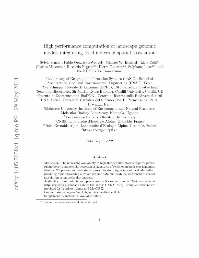
5 Results5.1 Population structureThe best partition of the dataset consisted of four populations, although the vast ma-jority of the samples were allocated to two clusters (almost 96%) on the basis of theancestry coefficients (Figure S1). Mapping these coefficients revealed the two clusters(340 and 431 individuals out of 804) occurred in the South-West and North-East ofUganda respectively. Using pictures of sampled individuals, the first cluster was iden-tified as Ankole cattle and the second one as zebu. The remaining two clusters (32animals) possibly represent introgression from allochthonous gene pools.

5.2 Detection of selection signaturesFour approaches were applied to detect selection signatures. The statistical significancethreshold for Samβada, LFMM and Arlequin was set to 1% before applying Bonferronicorrection. For BayEnv, model selection was based on the distribution of Bayes Factors(BF) for neutral loci (Coop et al., 2010). Results were analysed separately for eachenvironmental variable and models showing a BF higher than the 1st percentile of theneutral distribution were detected as candidate loci. For BayEnv and Arlequin, sampleswere classified into populations using a threshold of 0.85 for the higher admixture coeffi-cient, leading to three clusters of 162 Ankole cattle, 8 zebus and 10 cattle from the thirdpopulation; samples from the fourth population were highly admixed and none satisfiedthe condition.

Using univariate models, Samβada identified 2,499 SNPs (6.2 %) potentially subjectto selection, BayEnv 1977 (4.9 %), LFMM 280 (0.7 %) and Arlequin did not identifyany loci as significant. The loci detected by Samβada with the highest G scores werecompared among methods in table S2. Thirty-six loci were identified by the three cor-

8

relative methods and three of them were among the most significant models in Samβada(Table S3). These three SNPs occur close to each other in chromosome five.

Samβada’s multivariate analysis identified 84 significant bivariate models, corre-sponding to 29 loci. In Samβada’s framework, this means these models provided asignificantly more accurate estimation of the genotype’s frequency than their univari-ate parents, while at least one of their parents was also significant. Among those,three models that included the “population structure” variable also had a parent modelshowing a significant association with this variable. Therefore, although the popula-tion structure partly explains the distribution of these genotypes, adding an environ-mental variable provided a significantly more accurate estimation of their distribution(p ≤ 7.9 · 10−10 ⇔ G ≥ 37.8). These models correspond to three loci that were detectedby all correlative approaches.

5.3 Spatial autocorrelationGlobal and local indicators of spatial autocorrelation were computed for two genotypeswith a weighting scheme based on the 20 nearest neighbours: ARS-BFGL-NGS-113888(hereon ARS-113) (allele GG), which was detected by Samβada with the highest G scoreand was also detected by BayEnv, was compared with Hapmap28985-BTA-73836 (hereon HM-28) (allele GG), which was detected by Samβada, BayEnv and LFMM. Logis-tic models significantly associated both genotypes with isothermality, which measuresthe stability of temperature during the year. Figure 1 shows local indices of spatialautocorrelation for these 2 genotypes: on the one hand, ARS-113 (GG) was positivelyautocorrelated for the majority of points and the indicator was significant for half ofthem. The distribution of this marker shows spatial dependence, non-significant as-sociations were found at the edge of Lake Victoria and in a corridor in the North ofthe Lake with some occurrences in the West of Uganda. This widespread pattern ofspatial autocorrelation could originate from the underlying population structure, sinceAnkole cattle are more common in the South-West while zebus are more common in theNorth-East of the country. Thus the correlation detected by logistic regressions betweenARS-113 (GG) and environmental variables could be spurious and due to demographicfactors. On the other hand, the local indicators of spatial association of HM-28 (GG)showed lower values in general and were only significant in the North-West of Uganda.This particular region also showed the lowest values of isothermality in Uganda, i.e. ahigh variability of temperatures. The low value of spatial autocorrelation for HM-28(GG) implies that the distribution of this genotype was mostly independent from thelocation and this supports a possible adaptive origin of the observed correlation betweenHM-28 (GG) and isothermality with logistic models. This correlation between HM-28(GG) and isothermality also appeared with bivariate LISAs, where the presence of thegenotype was compared to the mean value of isothermality among neighbouring points(not shown).

9

(a) ARS-113 (GG) (b) HM-28 (GG)

Figure 1: Local indicators of spatial association of markers ARS-113 (allele GG) andHM-28 (allele GG). The weighting scheme is based on the first 20 nearest neighbours.Red points tend to be similar to their neighbours while blue points differ from them.Yellow points are independent from their neighbourhood. Small points indicate non-significant values (p > 0.001). The map in the background represents the relief, thedarker the shade, the higher the altitude. Samples coming from the same farm havebeen spread on a circle around their actual location.

10

6 DiscussionThe key features of Samβada are the multivariate modelling and the measure of spatialautocorrelation. Both can help the interpretation of results in the case that the datasetfeatures population structure. Bivariate models may include the global ancestry coeffi-cients provided by a preliminary analysis. This setup can detect which loci are correlatedwith the environment while taking demography into account. Additionally, the intro-duction of measurements of spatial autocorrelation into these analyses integrates spatialstatistics with landscape genomics. Contrary to most current and non-spatial models(e.g. Frichot et al., 2013; Coop et al., 2010), this approach integrated in Samβada allowsthe determination of whether the observed data reflects independent samples, a require-ment of the underlying modelling assumptions of such methodologies. Measuring spatialautocorrelation assesses whether the occurrence of a genotype is related to its frequencyin the surrounding locations. More specifically, local indices of spatial autocorrelationallow the mapping of areas prone to spatial dependency. On the basis of the presentanalysis, using spatial statistics in conjunction with correlative models may lower therisk of false positives due to population structure in landscape genomics.

In the present study, Samβada detected the highest number of SNPs as potentiallysubject to selection among the four approaches. However when comparing the positionsof these SNPs, 1,029 of them were less than 100,000 base pairs apart from another de-tected locus, thus some of these detections might refer to the same signature of selection.Samβada’s results partially match with those of BayEnv with 435 common SNPs (i.e.22% of BayEnv’s detections). Concerning the third correlative approach, LFMM is moreconservative than Samβada but the correspondence is better since 154 loci (out of 280,i.e. 55% of LFMM’s detections) are detected by both methods. Moreover, 25 SNPs de-tected by LFMM only are less than 100,000 base pairs apart from a loci detected bySamβada, potentially identifying the same selection signature. The order of detectionsdiffered between the two methods, as the most significant loci detected by Samβadaare ignored by LFMM. Lastly, Arlequin’s best results involved 17 SNPs with p-valueslower than 10−4 (significance threshold: α = 2.5 · 10−7), out of which 2 were commonwith Samβada and 16 were common with BayEnv. This result suggests that population-based methods, whether using outliers or environmental correlations, tend to detect thesame selection signatures. On the one hand, Samβada’s detection rate may indicatethe occurrence of some false positives due to population structure; on the other hand,the discrepancy between the results may indicate that the more conservative approacheshave some false negatives. Thus the actual number of loci subject to selection is likely tolie in between. Comparing the results in the light of spatial dependence gives informa-tion about the differences between Samβada’s and LFMM’s detections. Maps of localspatial autocorrelation for ARS-113 (GG) and HM-28 (GG) illustrated a general trend:LFMM discarded SNPs showing significant local spatial autocorrelation for a large pro-portion of the sampling locations, while Samβada detected them. Thus measuring localautocorrelation of candidate genotypes may help distinguishing between the effects oflocal adaptation and those of population structure among Samβada detections.

11

Regarding common detections, the three SNPs identified by Samβada when popu-lation structure was included as a covariate were among the common detections of cor-relatives approaches. Thus pre-existent knowledge on demography may be built on torefine correlation-based detections of selection signatures. One possible approach couldconsist of computing population structure and then including one variable summarisingthis structure in the constant model used by Samβada. This way, only genotypes show-ing a significant correlation with the environment while taking the population structureinto account would be detected. Concerning the biological function of the common de-tections, these three loci are located on chromosome 5, near the gene POLR3B whosemouse counterpart is involved in limiting infection by intracellular bacteria and DNAviruses (UniProt, www.uniprot.org). Moreover, genotype HM-28 (GG) shows spatialautocorrelation in the North-Western part of Uganda and this area overlaps with one ofthose where the higher load of tse-tse fly (Glossina spp.) occur in the country (Abilaet al. (2008); MAAIF et al., 2010). Hence the risk of cattle trypanosomiasis is high inthis region and the detected mutations may be involved in parasite resistance.

The increasing availability of large molecular datasets raises challenges regardingtheir analysis. Correlative approaches in landscape genomics enable fast detection ofcandidate loci to local adaptation. However these methods must take into account theeffect of population structure (Frichot et al., 2013; Joost et al., 2013; De Mita et al., 2013).Limited dispersal of individuals leads to spatial autocorrelation of marker frequencies,which may cause spurious correlations with the environment. Samβada addresses thefirst topic by detecting rapidly selection signatures and the second one by measuringthe level of spatial autocorrelation for candidate loci. The next methodological step in-volves developing spatially-explicit models that directly include autocorrelation. Guillotet al. (2014) provide such a model, however the current R-based implementation doesnot enable whole-genome analysis. Alternatively Geographically Weighted Regressions(GWR) measure the spatial stationarity of regression coefficients by fitting a distinctmodel for each sampling location. The number of neighbouring points considered foreach sampling location is given by the weighting scheme. These models allow some “lo-cal” coefficients to differ between sampling points while some “global” coefficients arecommon to all points (Fotheringham et al., 2002; Joost et al., 2013). Thus GWR enablesbuilding a null model where the constant term may vary in space and then refining itby adding a global environmental effect for all locations. Comparing these two modelswould enable an assessment of whether the global environmental effect is needed to de-scribe the distribution of the genotype. The key advantage of allowing the constant termto vary in space is to take spatial autocorrelation into account in the models. This way,GWR allows an investigation of the spatial behaviour of loci showing selection signaturewith standard logistic regressions and may help to distinguish between local adaptationand population structure in landscape genomics. However GWR models require a fine-tuning of the weighting scheme from the user, which restrains their application to verylarge datasets.

Computation time is critical when processing large datasets. In this context, Samβadais able to swiftly analyse high-density SNP-chips and variants from whole-genome se-

12

quencing (e.g. the case study presented in here is analysed within 69 minutes for uni-variates models alone and 8.5 hours for both univariate and bivariate models). Whenconsidering single-process computations, Samβada is approximately 4.5 times quickerthan LFMM and 30 times than BayEnv. Both Samβada and LFMM enable parallelisedprocessing. Samβada’s processing speed, combined with its ability to analyse the spa-tial autocorrelation in molecular data and to incorporate prior knowledge on populationstructure, suits a wide range of applications, especially those involving whole genomesequence data.

AcknowledgementFunding: This research is funded by EU FP7 project NextGen (Grant KBBE-2009-1-1-03).

The authors would like to thank Sergio Rey for his advices on assessing the signifi-cance of LISA, Stephan Morgenthaler for fruitful discussions on assessing the significanceof multivariate logistic models and Gilles Guillot for providing them with SGLMM fortesting purposes.

ReferencesAbila, P. P., Slotman, M. A., Parmakelis, A., Dion, K. B., Robinson, A. S., Muwanika,V. B., Enyaru, J. C. K., Lokedi, L. M., Aksoy, S., and Caccone, A. (2008). Highlevels of genetic differentiation between ugandan Glossina fuscipes fuscipes populationsseparated by lake kyoga. PLOS Neglected Tropical Diseases, 2(5), e242.

Alexander, D. H., Novembre, J., and Lange, K. (2009). Fast model-based estimation ofancestry in unrelated individuals. Genome Research, 19(9), 1655–1664.

Anselin, L. (1995). Local Indicators of Spatial Association - LISA. Geographical Analysis,27(2), 93–115. GISDATA (Geographic Information Systems Data) Specialist Meetingon GIS (Geographic Information Systems) and Spatial Analysis, Amsterdam, Nether-lands, Dec 01-05, 1993.

Beaumont, M. A. and Nichols, R. A. (1996). Evaluating loci for use in the genetic analysisof population structure. Proceedings Royal Society London B, 263, 1619–1626.

Colli, L., Joost, S., Negrini, R., Nicoloso, L., Crepaldi, P., Ajmone-Marsan, P., and Con-sortium, E. (2014). Assessing the spatial dependence of adaptive loci in 43 Europeanand Western Asian goat breeds using AFLP markers. PLOS ONE , 9(1).

Coop, G., Witonsky, D., Di Rienzo, A., and Pritchard, J. K. (2010). Using environmentalcorrelations to identify loci underlying local adaptation. Genetics, 185(4), 1411–1423.

13

De Mita, S., Thuillet, A.-C., Gay, L., Ahmadi, N., Manel, S., Ronfort, J., and Vigouroux,Y. (2013). Detecting selection along environmental gradients: analysis of eight meth-ods and their effectiveness for outbreeding and selfing populations. Molecular Ecology,22(5), 1383–1399.

Dobson, A. J. and Barnett, A. G. (2008). An Introduction to Generalized Linear Models.Chapman & Hall, 3 edition.

Excoffier, L. and Lischer, H. E. L. (2010). Arlequin suite ver 3.5: a new series of programsto perform population genetics analyses under Linux and Windows. Molecular EcologyRessources, 10(3), 564–567.

Farr, T. G., Rosen, P. A., Caro, E., Crippen, R., Duren, R., Hensley, S., Kobrick, M.,Paller, M., Rodriguez, E., Roth, L., Seal, D., Shaffer, S., Shimada, J., Umland, J.,Werner, M., Oskin, M., Burbank, D., and Alsdorf, D. (2007). The shuttle radartopography mission. Reviews of Geophysics, 45(2).

Foll, M. and Gaggiotti, O. (2008). A genome-scan method to identify selected lociappropriate for both dominant and codominant markers: A Bayesian perspective.Genetics, 180, 977–993.

Fotheringham, A. S., Brunsdon, C., and Charlton, M. (2002). Geographically WeightedRegression: the analysis of spatially varying relationships. John Wiley & Sons, Chich-ester, 1 edition.

Frichot, E., Schoville, S. D., Bouchard, G., and François, O. (2013). Testing for asso-ciations between loci and environmental gradients using latent factor mixed models.Molecular Biology and Evolution, 30(7), 1687–1699.

GDAL Development Team (2013). GDAL - Geospatial Data Abstraction Library, Version1.10 . Open Source Geospatial Foundation.

Guillot, G., Vitalis, R., le Rouzic, A., and Gautier, M. (2014). Detecting correlationbetween allele frequencies and environmental variables as a signature of selection. Afast computational approach for genome-wide studies. Spatial Statistics, 8, 145–155.

Günther, T. and Coop, G. (2013). Robust identification of local adaptation from allelefrequencies. Genetics, 195(1), 205–220.

Henry, P. and Russello, M. A. (2013). Adaptive divergence along environmental gradientsin a climate-change-sensitive mammal. Ecology and Evolution, 3(11), 3906–3917.

Hijmans, R., Cameron, S., Parra, J., Jones, P., and Jarvis, A. (2005). Very high res-olution interpolated climate surfaces for global land areas. International Journal OfClimatology, 25(15), 1965–1978.

Jones, M., Forester, B., Teufel, A., Adams, R., Anstett, D., Goodrich, B., Joost, S., andManel, S. (2013). Integrating spatially explicit approaches to detect adaptive loci ina landscape genomics context. Evolution, 67, 3455–3468.

14

Joost, S., Bonin, A., Bruford, M. W., Després, L., Conord, C., Erhardt, G., and Taberlet,P. (2007). A spatial analysis method (SAM) to detect candidate loci for selection:towards a landscape genomics approach to adaptation. Molecular Ecology, 16(18),3955–3969.

Joost, S., Kalbermatten, M., and Bonin, A. (2008). Spatial Analysis Method (SAM): asoftware tool combining molecular and environmental data to identify candidate locifor selection. Molecular Ecology Ressources, 8, 957–960.

Joost, S., Vuilleumier, S., Jensen, J. D., Schoville, S., Leempoel, K., Stucki, S., Widmer,I., Melodelima, C., Rolland, J., and Manel, S. (2013). Uncovering the genetic basis ofadaptive change: on the intersection of landscape genomics and theoretical populationgenetics. Molecular Ecology, 22(14), 3659–3665.

Ministry of Agriculture, Animal Industry and Fisheries, Uganda, Uganda Bureau ofStatistics, Food and Agriculture Organization of the United Nations, InternationalLivestock Research Institute, and World Resources Institute (2010). Mapping a betterfuture: Spatial Analysis and Pro-Poor Livestock Strategies in Uganda, pages 30–37.World Resources Institute, Washington, DC and Kampala.

Mitton, J. B., Linhart, Y. B., Hamrick, J. L., and Beckman, J. S. (1977). Observationson genetic structure and mating system of ponderosa pine in Colorado front range.Theoretical and Applied Genetics, 51(1), 5–13.

Moran, P. A. P. (1950). Notes on continuous stochastic phenomena. Biometrika, 37(1/2),pp. 17–23.

Pemstein, D., Quinn, K. M., and Martin, A. D. (2011). The Scythe statistical library: Anopen source C++ library for statistical computation. Journal of Statistical Software,42(12), 1–26.

Purcell, S., Neale, B., Todd-Brown, K., Thomas, L., Ferreira, M. A., Bender, D., Maller,J., Sklar, P., de Bakker, P. I., Daly, M. J., and Sham, P. C. (2007). PLINK: A tool setfor whole-genome association and population-based linkage analyses. The AmericanJournal of Human Genetics, 81(3), 559 – 575.

Vitalis, R., Dawson, K., Boursot, P., and Belkhir, K. (2003). DetSel 1.0: A computerprogram to detect markers responding to selection. Journal of Heredity, 94(5), 429–431.

Vitti, J. J., Grossman, S. R., and Sabeti, P. C. (2013). Detecting Natural Selection inGenomic Data. In Bassler, BL and Lichten, M and Schupbach, G, editor, AnnualReview of Genetics, Vol 47 , volume 47 of Annual Review of Genetics, pages 97–120.Annual Reviews, 4139 EL CAMINO WAY, PO BOX 10139, PALO ALTO, CA 94303-0897 USA.

Wright, S. (1949). The genetical structure of populations. Annals of Eugenics, 15(1),323–354.

15

High performance computation of landscape genomicmodels integrating local indices of spatial association

Supplementary material

1 Spatial autocorrelationSeveral indices are available for measuring the global spatial autocorrelation in a dataset. Samβadauses the Moran’s I (Moran, 1950), defined as follows:

I = n

S0

∑ni=1∑n

j=1 wij(yi − y)(yj − y)∑ni=1(yi − y)2 = n

S0

∑ni=1∑n

j=1 wijzizj∑ni=1 z2

i

(1)

avecn number of sampling points;wij weight of point j in the neighbourhood of i, defined by the spatial kernel;S0 sum of all weights

(S0 =

∑ni=1∑n

j=1 wij

);

yi, yj values for points i and j;y mean value;zi, zj deviations from the mean.

Local indices of spatial association (LISA, Anselin, 1995) measure the local association be-tween the value of a point and the neighbouring points. Samβada computes a local variant ofthe Moran’s I for each point i:

Ii = n − 1∑ni=1 z2

i

zi

n∑

j=1wijzj

(2)

(3)

LISAs are defined in such a way that their sum over all points is proportional to a globalmeasure of spatial autocorrelation, in this case the Moran’s I:

I = 1n − 1

n∑

i=1Ii (4)

1

arX

iv:1

405.

7658

v1 [

q-bi

o.PE

] 2

9 M

ay 2

014

2 Environmental variables

Variable Description Data sourceUsed forunivariateanalysis

Used forbivariateanalysis

alt_SRTM Altitude [m] SRTM3 X

aspect Orientation of the relief [◦] Derived fromSRTM3 X X

BIO2 Mean Diurnal Range

WorldClim

X X(Mean of monthly (max temp -min temp))

BIO3 Isothermality (BIO2/BIO7) (*100) X X

BIO7 Temperature Annual Range(max temp - min temp) X

BIO9 Mean Temperature of DriestQuarter X

BIO12 Annual Precipitation X X

BIO15 Precipitation Seasonality(Coefficient of Variation) X X

BIO18 Precipitation of WarmestQuarter X X

latitude Latitude Samplingmeasurements

X Xlongitude Longitude X Xprec2 Precipitation in February

WorldClim

Xprec3 Precipitation in March Xprec4 Precipitation in April X Xprec5 Precipitation in May X Xprec6 Precipitation in June Xprec7 Precipitation in July Xprec9 Precipitation in September Xprec10 Precipitation in October X Xprec11 Precipitation in November X X

slope Slope of the relief [%] Derived fromSRTM3 X X

tmin10 Minimal temperature in October WorldClim X Xtmax10 Maximal temperature in October X

Ankole Coefficient of ancestry to thepopulation Ankole

Analysis withAdmixture X

Number of variables 23 15

Table S1: Environmental variables used to detect selection signatures with correlative ap-proaches. Univariate analyses were performed with Sambada, BayEnv and LFMM and bivariateanalyses with Sambada

2

3 Population structure

Figure S1: Population structure computed with Admixture (Alexander et al., 2009). Individualsare gathered together by populations, labeled horizontally. The assignation is based on thehighest membership coefficient Qmax of the sample. Inside each population, individuals areranked by increasing (or decreasing) value of Qmax.

4 Computation times

41,215 SNPs 634,849 SNPs804 samples 102 samples

Samβada 1.2 2.9Samβada biv. 8.7 18.4BayEnv 41.3 62.,2LFMM 3.2 16.0LFMM (mono) 6.1 58.1Arlequin ? ?

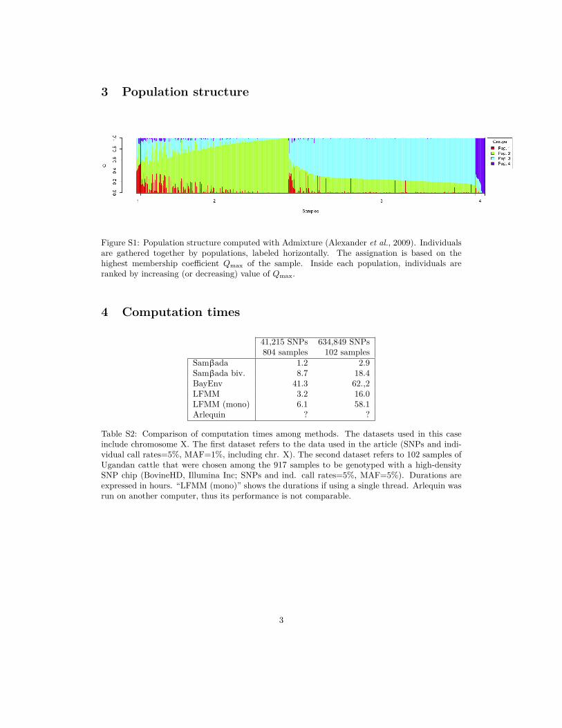
Table S2: Comparison of computation times among methods. The datasets used in this caseinclude chromosome X. The first dataset refers to the data used in the article (SNPs and indi-vidual call rates=5%, MAF=1%, including chr. X). The second dataset refers to 102 samples ofUgandan cattle that were chosen among the 917 samples to be genotyped with a high-densitySNP chip (BovineHD, Illumina Inc; SNPs and ind. call rates=5%, MAF=5%). Durations areexpressed in hours. “LFMM (mono)” shows the durations if using a single thread. Arlequin wasrun on another computer, thus its performance is not comparable.

3

5 Comparison of detections

Loci Chr. Pos. [Mbp] Samβ

ada

Bay

Env

LFM

M

Arle

quin

Detections1 ARS-BFGL-NGS-113888 5 48.32 1 1 0 0 22 Hapmap41074-BTA-73520 5 48.35 1 1 0 0 23 Hapmap41762-BTA-117570 5 18.94 1 1 0 0 24 ARS-BFGL-NGS-46098 20 2.95 1 1 0 0 25 Hapmap41813-BTA-27442 5 49.04 1 1 0 0 26 BTA-73516-no-rs 5 48.75 1 1 0 0 27 Hapmap28985-BTA-73836 5 70.34 1 1 1 0 38 Hapmap31863-BTA-27454 5 48.99 1 1 0 0 29 ARS-BFGL-NGS-106520 5 70.20 1 1 1 0 3

10 BTA-73842-no-rs 5 70.18 1 1 1 0 311 Hapmap50523-BTA-98407 5 46.74 1 1 0 0 212 BTB-01400776 20 2.70 1 1 0 0 213 Hapmap23956-BTA-36867 15 47.20 1 1 0 0 214 ARS-BFGL-NGS-10586 2 128.64 1 1 0 0 215 ARS-BFGL-NGS-43694 5 49.65 1 1 0 0 216 BTA-122374-no-rs 14 16.44 1 1 0 0 217 BTB-01356178 20 2.49 1 1 0 0 218 ARS-BFGL-NGS-94862 11 103.53 1 1 1 0 319 BTA-108359-no-rs 14 16.31 1 0 0 0 120 ARS-BFGL-NGS-15960 5 28.02 1 1 0 0 221 ARS-BFGL-NGS-116294 2 128.58 1 1 0 0 222 INRA-566 13 57.94 1 0 1 0 223 BTA-49720-no-rs 5 69.66 1 1 1 0 324 ARS-BFGL-NGS-56387 13 24.36 1 1 0 0 225 BTA-28185-no-rs 26 22.78 1 0 0 0 1

Table S3: List of SNPs detected by Samβada corresponding to the models with the highest Gscores. Loci are identified by their name, their chromosome and their position in million basepairs. The following columns show which method detected them and the last one counts thesedetections. Loci in bold type are the commons discoveries of Samβada, LFMM and BayEnv.Local indices of spatial autocorrelation were computed for SNPs on lines 1 and 7.

ReferencesAlexander, D. H., Novembre, J., and Lange, K. (2009). Fast model-based estimation of ancestryin unrelated individuals. Genome Research, 19(9), 1655–1664.

Anselin, L. (1995). Local Indicators of Spatial Association - LISA. Geographical Analysis,27(2), 93–115. GISDATA (Geographic Information Systems Data) Specialist Meeting on GIS(Geographic Information Systems) and Spatial Analysis, Amsterdam, Netherlands, Dec 01-05,1993.

Moran, P. A. P. (1950). Notes on continuous stochastic phenomena. Biometrika, 37(1/2), pp.17–23.

4