High-Order Accurate Fluid-Structure Simulation of a Tuning Fork

Bradley Froehlea, Per-Olof Perssona,∗

aDepartment of Mathematics, University of California, Berkeley, Berkeley, CA 94720-3840, USA

Abstract

The aeroacoustics of a tuning fork are investigated using a high-order fluid-structure interaction (FSI)scheme. The compressible Navier-Stokes equations are discretized using a discontinuous Galerkin arbitraryLagrangian-Eulerian (DG-ALE) method on an unstructured tetrahedral mesh, and coupled to a non-linearhyperelastic neo-Hookean model of a tuning fork, discretized using continuous Galerkin finite elements on anunstructured tetrahedral mesh. The fluid and structure are both integrated implicitly in time using a parti-tioned approach based on an implicit-explicit Runge-Kutta method. We measure radial sound distributionswhich show good agreement with theoretical predictions and physical experiments in the open literature.In addition we demonstrate how to measure Q factors for several common modes, emphasizing that we canaccurately capture the decay rates arising purely from the interaction of the tuning fork with the air andwithout any damping built into the structure model.

Keywords: Aeroacoustics, discontinuous Galerkin, Fluid-structure interaction, tuning fork

1. INTRODUCTION

There has been growing interest in using physical models based on the fundamental laws of mechanicsto describe and study the acoustics of musical instruments. This field is broadly split into two categories,depending on the mechanism of sound generation.

The first category includes recorders [1, 2, 3], flutes [4], organs [5], and other wind instruments. Herethe motion of air is often quite complex and models generally require the use of the Navier-Stokes equationsto properly capture the mechanism of sound generation. Recent work has included so-called direct numer-ical simulations in which the entire domain is modeled using the Navier-Stokes equations and the soundpropagation read directly from the resulting pressure field.

The second category contains instruments which vibrate to produce pressure waves, perhaps with thehelp of soundboards or resonator cavities. Notable past work in this category includes guitars [6], pianos[7], and other stringed instruments [8]. Here one generally creates a model for the strings, soundboard, andresonator cavity which is then coupled to a fluid model to capture the acoustic propagation. The fluid modelis generally simple, obtained, for example, by linearizing the Euler or Navier-Stokes equations assuming smallperturbations of a constant solution. This typically results in a system of equations analogous to Maxwell’sequations and which are solved using a finite-difference time-domain method [9].

Here we propose a direct numerical simulation of a three dimensional tuning fork, modeling the fluidusing the compressible Navier-Stokes equations and the structure with a neo-Hookean non-linear elasticitymodel. By using high-order spatial discretizations of both the fluid and structure domains, together witha high-order temporal integration based upon an implicit-explicit Runge-Kutta method, we can accuratelycapture the process of sound generation and natural decay rates of the system.

The tuning fork has long been studied. Helmholtz, for instance, observed that the sound generation isnot directionally uniform near the tuning fork. Instead, in Ref. [10] (page 161), Helmholtz observes:

∗Corresponding author. Tel.: +1-510-642-6947; Fax.: +1-510-642-8204.Email addresses: bfroehle@berkeley.edu (Bradley Froehle), persson@berkeley.edu (Per-Olof Persson)

Preprint submitted to Computers & Fluids March 24, 2015

4.0 8.5

110

0.5

0.9E = 200 GPa

ν = 0.29

ρ = 7.8 gm/cm3

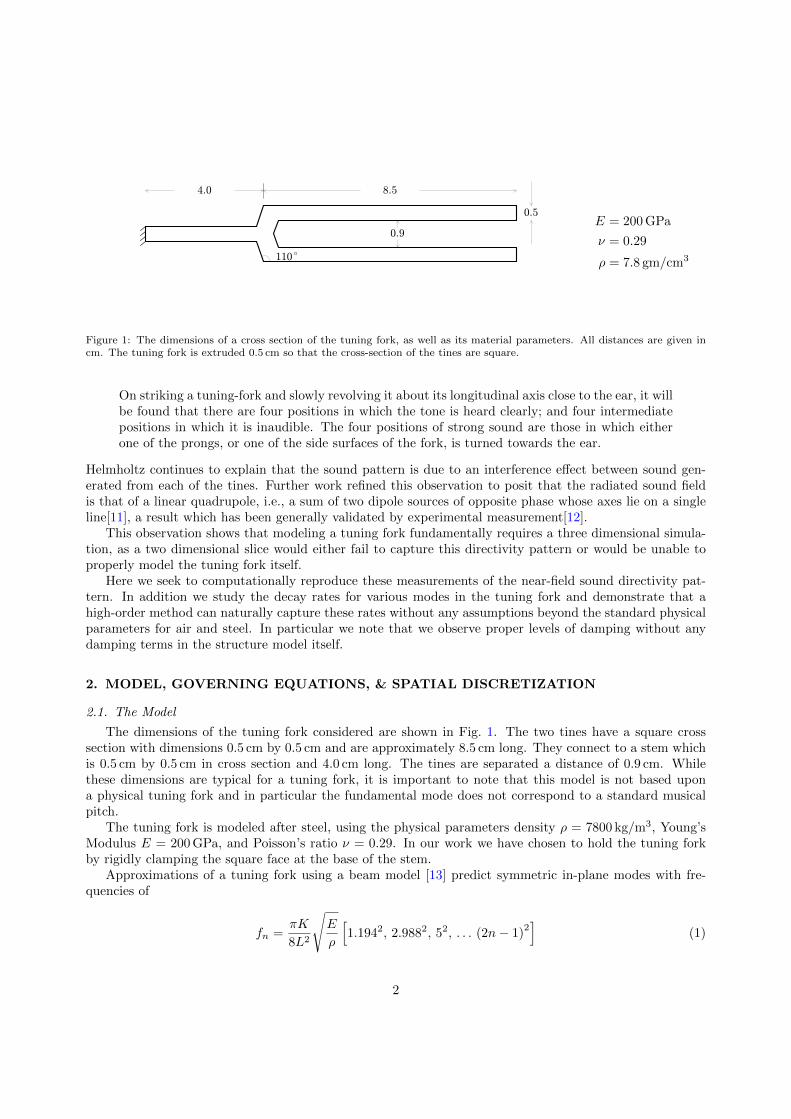
Figure 1: The dimensions of a cross section of the tuning fork, as well as its material parameters. All distances are given incm. The tuning fork is extruded 0.5 cm so that the cross-section of the tines are square.

On striking a tuning-fork and slowly revolving it about its longitudinal axis close to the ear, it willbe found that there are four positions in which the tone is heard clearly; and four intermediatepositions in which it is inaudible. The four positions of strong sound are those in which eitherone of the prongs, or one of the side surfaces of the fork, is turned towards the ear.

Helmholtz continues to explain that the sound pattern is due to an interference effect between sound gen-erated from each of the tines. Further work refined this observation to posit that the radiated sound fieldis that of a linear quadrupole, i.e., a sum of two dipole sources of opposite phase whose axes lie on a singleline[11], a result which has been generally validated by experimental measurement[12].

This observation shows that modeling a tuning fork fundamentally requires a three dimensional simula-tion, as a two dimensional slice would either fail to capture this directivity pattern or would be unable toproperly model the tuning fork itself.

Here we seek to computationally reproduce these measurements of the near-field sound directivity pat-tern. In addition we study the decay rates for various modes in the tuning fork and demonstrate that ahigh-order method can naturally capture these rates without any assumptions beyond the standard physicalparameters for air and steel. In particular we note that we observe proper levels of damping without anydamping terms in the structure model itself.

2. MODEL, GOVERNING EQUATIONS, & SPATIAL DISCRETIZATION

2.1. The Model

The dimensions of the tuning fork considered are shown in Fig. 1. The two tines have a square crosssection with dimensions 0.5 cm by 0.5 cm and are approximately 8.5 cm long. They connect to a stem whichis 0.5 cm by 0.5 cm in cross section and 4.0 cm long. The tines are separated a distance of 0.9 cm. Whilethese dimensions are typical for a tuning fork, it is important to note that this model is not based upona physical tuning fork and in particular the fundamental mode does not correspond to a standard musicalpitch.

The tuning fork is modeled after steel, using the physical parameters density ρ = 7800 kg/m3, Young’sModulus E = 200 GPa, and Poisson’s ratio ν = 0.29. In our work we have chosen to hold the tuning forkby rigidly clamping the square face at the base of the stem.

Approximations of a tuning fork using a beam model [13] predict symmetric in-plane modes with fre-quencies of

fn =πK

8L2

√E

ρ

[1.1942, 2.9882, 52, . . . (2n− 1)

2]

(1)

2

Figure 2: The tuning fork (gray) inside the computational domain.

where L is the length of the tines and K is the radius of gyration (1/√

12× 0.5 cm in our case). Using thephysical parameters for steel, this gives approximate values of the first two frequencies:

f1 ≈ 566.3 Hz and f2 ≈ 3546 Hz. (2)

As is customary, we will refer to the first mode as the fundamental or principal mode. This is the dominantmode when the tuning fork is struck and corresponds to the pitch that is heard. In this mode the two tinesmove in a symmetrical fashion — at any moment either both towards each other or both away from eachother. The second mode is called the clang mode and corresponds to a symmetric mode where the tips ofthe tines move towards each other while the middle of the tines move away from each other, and vice versa.

In addition to symmetric in-plane modes, there are also a few other natural classes of modes. Asymmetricin-plane modes are ones where the tines of the tuning fork move in the same direction. Here it is difficultto have a theoretical formula for the frequencies because the stem also plays a large role in the motion.Out-of-plane modes are ones where the tines of the tuning fork leave the plane, either in a symmetrical orasymmetrical fashion.

Before moving on we finally note that we model the tuning fork as immersed in air. The air is assigned typ-ical values: density ρ = 1.24 kg/m3, speed of sound c = 343.0 m/s, and dynamic viscosity 1.836·10−5kg/(m s).The simulation domain is a box which extends 10 cm from the tuning fork in each of the Cartesian directions.More specifically the tuning fork is centered in a box of dimension 32.5 cm × 21.9 cm × 20.5 cm. Note thatthis domain is almost entirely near-field, as the wavelengths for the two symmetric in-plane modes (eq. 2)are:

λ1 = 60.5 cm and λ2 = 9.67 cm. (3)

These lengths are both on the order of, or larger than, the size of the computational domain. A schematicof the tuning fork and the domain is shown in Fig. 2.

3

2.2. Compressible Navier-Stokes

The air is modeled using the compressible Navier-Stokes equations, which are a non-linear system ofequations which can be written in conservation form as:

∂

∂t(ρ) +

∂

∂xj(ρuj) = 0 (4)

∂

∂t(ρui) +

∂

∂xj(ρuiuj + pδij) = +

∂

∂xjτij for i = 1, 2, 3 (5)

∂

∂t(ρE) +

∂

∂xj(ρujE + ujp) =

∂

∂xj(−qj + uiτij) (6)

where the conserved variables are the fluid density ρ, momentum in the j-th spatial coordinate directionρuj , and total energy ρE. The viscous stress tensor and heat flux are given by

τij = µ

(∂ui∂xj

+∂uj∂xi− 2

3

∂uk∂xk

δij

)and qj = − µ

Pr

∂

∂xj

(E +

p

ρ− 1

2ukuk

). (7)

Here, µ is the dynamic viscosity and Pr = 0.72 is the Prandtl number which we assume to be constant. Foran ideal gas, the pressure p has the form

p = (γ − 1)ρ

(E − 1

2ukuk

), (8)

where γ = 1.4 is the adiabatic gas constant. We impose an adiabatic no-slip boundary condition on theboundary with the tuning fork. The far walls of the simulation domain should represent an infinite do-main, i.e., be perfectly absorbing. However here we use a characteristic free-stream type boundary whichis a first-order approximation of the out-going wave condition. For this problem, this appears to be suf-ficiently accurate, and we have not observed any spurious modes corresponding to the dimensions of thecomputational domain.

2.3. Arbitrary Lagrangian Eulerian formulation

The deformable fluid domain is handled through an Arbitrary Lagrangian Eulerian (ALE) formulation.In this method, a simple change of variables reduces the complexity introduced by the variable geometryto that of solving a transformed conservation law on a fixed reference mesh. In particular, no remeshing orinterpolation is required as the domain deforms.

Here a point X in a fixed reference domain V is mapped to x(X, t) in a time-varying domain v(t). Thedeformation gradient G, mapping velocity ν, and mapping Jacobian g are defined as

G = ∇Xx, ν =∂x

∂t, and g = detG. (9)

A system of conservation laws in the physical domain (x, t)

∂u

∂t+∇x · f(u,∇xu) = 0 (10)

is rewritten as a system of conservation laws in the reference domain (X, t)

∂U

∂t+∇X · F (U ,∇XU) = 0 (11)

where the conserved quantities and fluxes in reference space are

U = gu, F = gG−1f − uG−1ν. (12)

4

The equations are discretized in space using a high-order discontinuous Galerkin formulation with tetra-hedral mesh elements and nodal basis functions. The inviscid fluxes are computed using Roe’s method [14],and the numerical fluxes for the viscous terms are chosen according to the compact discontinuous Galerkin(CDG) method [15]. There are many other options for numerical fluxes, see e.g. references [16, 17], and wedo not expect the choice to be significant in our study. After discretizing, we obtain the semi-discrete formof our equations:

Mf duf

dt= rf (uf ; x), (13)

for solution vector uf , mass matrix Mf , and residual function rf (uf ; x). Observe that we have writtenthe residual function in such a way as to highlight the dependence on the ALE mesh motion x. For moredetails see reference [18].

The geometric conservation law (GCL) can be enforced using a simple technique involving an auxiliaryequation. However, since the experiments in reference [18] indicate that high-order approximation spacesare less sensitive to the GCL condition, we are for simplicity not enforcing it in our results here.

2.4. Neo-Hookean Elasticity Model

We use a non-linear hyperelastic neo-Hookean formulation [19] to model the tuning fork. Here, thestructure position is given by a mapping x(X, t), which for each time t maps a point X in the unstretchedreference configuration to its location x in the deformed configuration. From this we compute the mappingvelocity v and deformation gradient F as

v =∂x

∂tand F = ∇Xx(X, t). (14)

Note that F here is not the Navier-Stokes flux function as defined in the previous subsection.We partition boundary of the structure domain into regions of Dirichlet and Neumann boundary condi-

tions, ∂V = ΓD ∪ ΓN . On the Dirichlet boundary ΓD (i.e., the base of the tuning fork) we prescribe thematerial position xD, or equivalently the material velocity vD. On the Neumann boundary ΓN we allow fora general surface traction (i.e., force per unit surface area) which we denote t.

The governing equations for the structure are

∂p

∂t−∇ · P (F ) = b in Ω (15)

P (F ) ·N = t on ΓN (16)

x = xD on ΓD (17)

where p = ρv = ρ ∂x/∂t is the momentum, P is the first Piola-Kirchhoff stress tensor, b is an external bodyforce per unit reference volume, and N is a unit normal vector in the reference domain.

For a compressible neo-Hookean material the strain energy density is given by

W =µ

2(I1 − 3) +

κ

2(J − 1)

2(18)

where I1, the first invariant of the deviatoric part of the left Cauchy-Green deformation tensor, and J , thedeterminant of the deformation gradient, are calculated as

I1 = J−2/3I1, I1 = trB = tr(FF T ), and J = detF . (19)

The constants µ and κ are the shear and bulk modulus of the material.The first Piola-Kirchhoff stress tensor is computed as

P (F ) =∂W

∂F= µJ−2/3

(F − 1

3tr(FF T )F−T

)+ κ(J − 1)JF−T . (20)

5

After writing the system in a first order formulation in the displacement x and momentum p variables,the equations are discretized in space using a standard high-order continuous Galerkin formulation withtetrahedral mesh elements and nodal basis functions. This results in a semi-discrete system:

M s dus

dt= rs(us; t), (21)

for solution vector us containing discretized positions and momenta, mass matrix M s, and residual functionrs(us; t) where again t is a surface traction (and not time). Note in this form it is most natural to imposethe Dirichlet conditions in the momentum variables only, letting them be integrated into the correspondingchanges in position.

3. COUPLING & TEMPORAL DISCRETIZATION

3.1. Coupling / Radial Basis Functions

The coupling between the fluid and structure is simplified by creating fluid and structure meshes whichare conformal along the fluid-structure interface. By this, we mean that there is a one-to-one mappingbetween the boundary faces of each mesh on the shared interface. In addition we discretize the fluid andstructure using elements of the same polynomial order to ensure that the deformed fluid domain can exactlyconform to the deformed structure.

To compute the fluid-to-structure coupling we numerically evaluate the momentum flux through theboundary faces and provide the quantities to the structure solver as the surface traction. To ensure a highlyaccurate coupling this transfer is done at the Gaussian integration nodes, not the solution nodes.

The structure-to-fluid coupling is a deformation of the fluid mesh in response to a change in the structureposition. We represent the deformed fluid mesh and mapping velocity on each element of the fluid mesh usingpolynomials of the same order as the fluid discretization. Since we insist that the fluid and structure arediscretized using the same order polynomials, the deformed fluid mesh may exactly conform to the deformedstructure by setting the positions of the boundary fluid nodes to the deformed position of the structure.Since the structure may undergo a large deformation, we use radial basis function interpolation [20, 21] todeform the fluid mesh to maintain high element quality and prevent element inversion.

The radial basis function interpolant gives the deformed fluid position x as a function of the referenceposition X and has the form

x(X) =

n∑j=1

αjφ(‖X −Xj‖2/r0) + p(X) (22)

where Xj is a set of control points, φ is a radial basis function, r0 is a characteristic distance, and p is alinear polynomial. Here we choose a compactly supported C2 function

φ(r) =

(1− r)4(4r + 1) if 0 ≤ r ≤ 1

0 if 1 ≤ r.(23)

The coefficients αj and coefficients of the polynomial p are found by solving the linear system

xj = x(Xj) for j = 1, . . . , N (24)

0 =

N∑j=1

αjq(Xj) for all linear polynomials q (25)

where the control points Xj are set to be all nodes on the boundary of the fluid mesh and their controlvalues xj are either the current displacement of the structure or the reference location depending onwhether the node is along the fluid-structure interface or at a far boundary.

6

3.2. Temporal Integrator

Consider for the moment our system of fluid uf and structure us variables written as a coupled firstorder system of ordinary differential equations

Mf duf

dt= rf (uf ; x(us)) (26)

M s dus

dt= rs(us; t(uf )). (27)

where we explicitly show the coupling as arising through the ALE mesh motion x and surface traction t.We integrate the system using a high-order predictor-corrector method based upon an implicit-explicit

(IMEX) Runge-Kutta scheme, where in essence the fluid-to-structure coupling is integrated explicitly andthe remaining terms in the system are integrated implicitly. Here we use the ARK3 coefficients of Kennedyand Carpenter [22] which is a 4 stage method. We use standard notation, letting s denote the number ofstages, and aij , aij , bi, and ci denote the coefficients of the implicit scheme, explicit scheme, weights, andnodes respectively.

The time integration scheme is written out fully in algorithm 1. For more details see references [23, 24,25, 26].

Algorithm 1 Time integration scheme for the FSI system in equations 26 and 27, using the s-stage implicit-explicit Runge-Kutta scheme (aij , aij , bi, ci). Given the structure (usn) and fluid (ufn) values at time tn,compute the values at tn+1 = tn + ∆t.

Set tn,1 = t(ufn,1) . Evaluate fluid-to-structure coupling (surface traction)

Set ksn,1 = M−1s rs(usn,1; tn,1) . Evaluate structure residual

Set kfn,1 = M−1f rf (ufn,1; x(usn,1)) . Evaluate fluid residual

for stage i = 2, . . . , s doSet tn,i =

∑i−1j=1

aij−aijaii

tn,j . Predict the fluid-to-structure coupling

Solve for ksn,i in Msksn,i = rs(usn,i; tn,i) . Implicit structure solve

where usn,i = usn + ∆t∑ij=1 aijk

sn,j

Solve for kfn,i in Mfkfn,i = rf (ufn,i; x(usn,i)) . Implicit fluid solve

where ufn,i = ufn + ∆t∑ij=1 aijk

fn,j

Set tn,i = t(ufn,i) . Correct the fluid-to-structure coupling

Set ksn,i = M−1s rs(usn,i; tn,i) . Re-evaluate structure residual

end forSet usn+1 = usn + ∆t

∑si=1 bik

sn,i . Advance structure

Set ufn+1 = ufn + ∆t∑si=1 bik

fn,i . Advance fluid

4. RESULTS

Finally, we present results for a single three-dimensional tuning fork simulation. We created two un-structured tetrahedral meshes, one for the fluid and structure. The structure mesh contained about 2,200tetrahedra which for our polynomial degree p = 3 gives about 13,600 high-order nodes, or 82,000 degreesof freedom. The fluid mesh consisted of approximately 23,200 tetrahedra which for our polynomial degreep = 3 gives 464,000 high-order nodes, or 2,320,000 degrees of freedom (see Fig. 3). Using these meshes theequations of motion for the tuning fork and fluid were discretized in space as described in sections 2.2–2.4.

The tuning fork was initialized by linearly skewing the tines apart from each other so that at the tip theinterior spacing increased by 0.014 cm and the exterior spacing increased by 0.029 cm. We note that this isa highly nonphysical excitation, but was intended to validate the robustness of the solver and ensure that

7

(a) Along the tuning fork axis. (b) Perpendicular to the tuning fork axis.

Figure 3: The computational mesh for the tuning fork (green) and two different cross sections of the computational mesh forthe fluid (blue) in a region near the tuning fork.

many of the symmetrical modes of the tuning fork would be excited. The tines were then released and thesystem integrated in time using the algorithm in section 3.2. A timestep of ∆t = 50µs was used and thesystem was solved until T = 30 ms for a total of 600 time steps. This timestep corresponds to a samplingfrequency of 20 kHz allowing us to resolve frequencies below 10 kHz. We note that this timestep correspondsto a CFL number of approximately 100 for the fluid, compared to an explicit RK4 scheme, based on thesound speed and the size of the smallest elements.

Because of rather severe initial transients due to the highly deformed configuration of the structure, atimestep of ∆t/5 was used for the first 5 timesteps. Each time step took approximately one minute on 768processors, for a total simulation time of approximately 10 hours.

4.1. Pressure Time Series

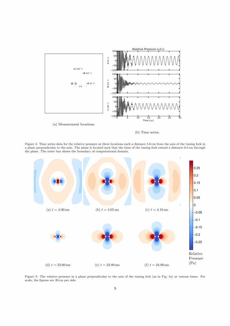
We measured the pressure at several locations surrounding the tuning fork, in each case recording thevalue relative to the baseline pressure p0 = 1.012× 105 Pa. In Fig 4 we present a time series for the pressureat three locations, each in a plane perpendicular to the axis of the tuning fork intersecting the tuning fork0.5 cm away from the tips of the tines. The locations shown are all a distance of 5.0 cm from the axis of thetuning fork, making angles of 0, 45, and 90 with the axis which passes through both tines. Observe thatthe high frequency modes decay quickly over the first 10 ms or so, leaving a signal which is almost entirelycomposed of the principal frequency.

We also present cross sectional visualizations of the pressure at two representative sequences of frames inFig. 5. The first sequence, 4.00 ms to 4.10 ms, is before the initial transients have decayed. In this sequencewe can see that a high frequency mode, most likely the clang mode, is dominant. In the second sequence,23.60 ms to 24.00 ms, we see approximately one quarter period of the fundamental mode.

Recall that the sound pressure level Lp, measured in dB above a standard reference level, is calculatedas

Lp = 10 log10

(prms

2

pref2

), (28)

where prms is the root mean square of the signal (relative to the baseline pressure) and pref is a referencepressure typically set to 2×10−5 Pa [27]. By taking a Fourier transform of the last 9 periods of the pressuresignal at location A, we show the sound pressure level for various frequency in Fig 6. In addition welinearized the tuning fork model around the reference configuration (in the absence of air) and show severalcomputed eigenfrequencies with a description of their corresponding eigenmodes. Due to the comparativelyshort length of time simulated, the resolution from the Fourier transform is somewhat lacking especially inthe low frequency regime. We will return to this point later in section 4.4.

8

A (0 )

B (45 )

C (90 )

5.0

(a) Measurement locations.

100

50

0

50

100

A (

0)

Relative Pressure (mPa)

100

50

0

50

100

B (

45)

0 5 10 15 20 25 30Time (ms)

100

50

0

50

100

C (

90)

(b) Time series.

Figure 4: Time series data for the relative pressure at three locations each a distance 5.0 cm from the axis of the tuning fork ina plane perpendicular to the axis. The plane is located such that the tines of the tuning fork extend a distance 0.5 cm throughthe plane. The outer box shows the boundary of computational domain.

(a) t = 4.00 ms (b) t = 4.05 ms (c) t = 4.10 ms

(d) t = 23.60 ms (e) t = 23.80 ms (f) t = 24.00 ms

−0.25

−0.2

−0.15

−0.1

−0.05

0

0.05

0.1

0.15

0.2

0.25

RelativePressure(Pa)

Figure 5: The relative pressure in a plane perpendicular to the axis of the tuning fork (as in Fig. 4a) at various times. Forscale, the figures are 20 cm per side.

9

100 200 500 1000 2000 5000 10000Frequency (Hz)

40

20

0

20

40

60

80

Sound P

ress

ure

Level (d

B)

f=195.6 Hz

Asymmetricin-plane

f=564.9 Hz

Fundamentalmode

f=1463.2 Hz

Asymmetricin-plane

f=3484.3 Hz

Clangmode

Frequency Spectrum at location A (0 )

Figure 6: The sound pressure level Lp relative to a reference pressure 2 × 10−5 Pa for a range of frequencies, as measuredover the last 9 periods of the base frequency as observed at location A. The frequencies of several eigenmodes of the linearizedstructure are shown for comparison.

4.2. Angular Dependence

The directionality of the sound field radiated by a tuning fork may also be measured. The tuning forkis thought to be well modeled by a linear quadrupole, i.e., two dipoles of opposite phase whose dipole axeslie along a single line. A formula for the resulting pressure field is derived as [11, 12]

p(r, θ) =A

r

[(1− 3 cos2 θ)

(ik

r− 1

r2+k2

3

)− k2

3

](29)

where A is a normalization constant, r is the distance from the linear quadrupole source, k = 2π/λ isthe wave number, and i indicates an out-of-phase term. The product kr is generally used to separate theso-called near-field kr 1 from the far-field kr 1.

From this formula we compute the angular and radial dependence on the sound pressure level for anidealized linear quadrupole:

Lp = 10 log10

(‖p(r, θ)‖2

pref2

). (30)

In Fig. 7, we compare this idealized angular dependence to measured sound pressure levels at a variety ofdistances from the axis of the tuning fork. In each case the measurements were done in the same plane asour previous measurements (see Fig. 4a). As is typical, we have normalized each plot to the maximum valueso that the maximum sound pressure level is shown as 0 dB.

Perhaps the most striking aspect of the directivity plots is the sharp decrease in sound pressure levelsbetween regions of maxima. For instance, we observe a SPL drop of over 40 dB for 4 specific angles whenmeasuring 2.5 cm away from the axis of the tuning fork. Next observe that we accurately capture theexpected 5 dB drop in the maximum sound pressure level between the 0–180 and the 90–270 axes.

Also notable is the relatively good agreement between the measured sound pressure levels and the linearquadrupole source behavior, especially at the larger radii of 7.5 cm and 10.0 cm. For smaller radii the system

10

0°

30°

60°90°

120°

150°

180°

210°

240°270°

300°

330°

-40 -30 -20 -10 0dB

(a) 2.5 cm

0°

30°

60°90°

120°

150°

180°

210°

240°270°

300°

330°

-40 -30 -20 -10 0dB

(b) 5.0 cm

0°

30°

60°90°

120°

150°

180°

210°

240°270°

300°

330°

-40 -30 -20 -10 0dB

(c) 7.5 cm

0°

30°

60°90°

120°

150°

180°

210°

240°270°

300°

330°

-40 -30 -20 -10 0dB

(d) 10.0 cm

Figure 7: The relative sound pressure levels by angle at various distances from the axis of the tuning fork measured in 1

increments, averaged over nine periods of the fundamental mode. Each plot has been normalized to its maximum value. Thetheoretical curve for a linear quadrupole as given in Eq. 29 is shown in a solid line. The tines of the tuning fork lie at 0 and180. Notice the 5 dB difference in sound pressure level between the two maxima in the extreme near-field.

11

is likely no-longer well-modeled by an idealized linear quadrupole as the finite size effects of the actual tuningfork are likely to play a larger role. We note that our observed disparity between measurements and thelinear quadrupole at 2.5 cm has a similar character to previous experimental measurements (c.f., Fig. 9bin Ref. [12]) wherein the lobes at 90 and 270 are observed to be wider than those of an idealized linearquadrupole, and the lobes at 0 and 180 are observed to be narrower.

4.3. Quality Factor

A major quantity of interest in a resonator system is the Q factor or quality factor. There are twoequivalent definitions for the Q factor, one based on energy storage and losses and another based on resonancebandwidth. Here we consider the former, defining the Q factor as

Q = 2πE

∆E(31)

where E is the total energy stored in the resonator and ∆E is the energy dissipated per cycle. Since∆E E, a bit of algebra shows that we can equivalently define the Q factor as the number of periodsrequired for the energy to decay by e−2π. In other words, Q = 2πfτ if the energy signal decays like e−t/τ .Since we have seen that the tuning fork emits an almost entirely pure signal at the fundamental frequencyafter 10 ms, we will consider 1 cycle to be one period of the fundamental mode.

We calculate the total energy of the tuning fork as

E =

∫V

W dx︸ ︷︷ ︸potential

+

∫V

1

2ρv2 dx︸ ︷︷ ︸

kinetic

(32)

where V is the reference configuration, ρ is the reference density, v is the material velocity, and W is thestrain energy density as defined in equation 18.

We show the potential, kinetic, and total energy contained within the tuning fork as a function of timein Fig. 8a. Note the large initial losses due to the decay of high-frequency transients followed by a region oflittle decay. By changing the scale of the vertical axis we can better highlight the slow decay of the energyin the tuning fork, as shown in Fig. 8b. Here we have fit an exponential decay curve to the total energyfor the values after 10 ms. We see that the best fit curve quite closely approximates the decay in energyover many cycles, with only some small intra-cycle deviations as the tuning fork does not emit energy at aconstant rate.

The best fit exponential has the form E ≈ A exp(−t/τ) where we find A = 0.798 mJ and τ = .96 s. Sincethe fundamental frequency is f = 564 Hz we easily calculate the Q factor to be 3400 which is in the rangeexpected for a tuning fork.

4.4. Filter Diagonalization & Harmonic Inversion

Another way to measure the Q factor is by running the pressure time series through a so-called harmonicinversion process. Here we approximate the pressure by a sum of decaying exponential functions:

p(t) ≈∑k

dke−iωkt (33)

with complex-valued parameters dk and ωk, where ωk encodes the resonant frequency and Q factor of thek-th mode.

There are many such ways to create such a series. For example, the Fourier transform (Fig. 6) is alreadysuch a series, however its numerical stability comes at the expense of poor frequency resolution because theωk are fixed with a linear spacing of O(1/T ) where T is the duration of the time series.

Here we employ the filter diagonalization method [28, 29, 30], using the freely available Harminv software[31]. We use the pressure time series data from location A (see Fig. 4a) as the input signal and specify afrequency window of 100 Hz to 10, 000 Hz. The method identifies the fundamental frequency f = 562.6 Hz

12

0 5 10 15 20 25 30Time (ms)

0.0

0.5

1.0

1.5

2.0

Energ

y (

mJ)

PotentialKineticTotal

(a) Energy time series.

0 5 10 15 20 25 30Time (ms)

0.770

0.775

0.780

0.785

0.790

0.795

0.800

0.805

0.810

Energ

y (

mJ)

Total EnergyBest fit

(b) Zoomed in view with a best-fit curve.

Figure 8: Kinetic, potential, and total energy of the tuning fork.

13

Frequency (Hz) Q Factor Notes

196.0 453.1 Asymmetric in-plane562.2 3414.0 Fundamental mode

1459.0 194.8 Asymmetric in-plane3424.0 22.8 Clang mode

Table 1: Significant frequencies and Q factors observed in the time series pressure data at location A (see Fig. 4a) during5.0 ms ≤ t ≤ 30.0 ms, as extracted by the filter diagonalization method.

with corresponding Q factor 3414.0. In addition, several other modes are well resolved and are shown intable 1. These modes include the clang mode and two asymmetric in-plane modes, each of which has a muchsmaller Q factor than the fundamental mode. Note that the identified frequencies are in good agreementwith the modes predicted by the linear eigenvalue analysis as shown in Fig. 6.

5. CONCLUSIONS

In this paper we have demonstrated how high-order fluid-structure interaction methods can accuratelycapture the dynamics of a tuning-fork, providing accurate predictions of frequencies, angular sound pressurelevel distributions, Q factors, and damping rates.

Future work includes more realistic initial conditions (e.g., an impulsive hit with a mallet), a largercomputational domain for far-field measurements, improved absorbing boundary conditions on the far walls,and the addition of a resonance box. In addition more work could be done to explore the higher symmetricmodes as well as the asymmetric and out-of-plane modes.

Lastly we mention that techniques similar to the ones used in this paper could be used to simulate avariety of other instruments including gongs, xylophones, and marimbas.

References

[1] Obikane Y, Kuwahara K. Direct simulation for acoustic near fields using the compressible navier-stokes equation. In:Choi H, Choi HG, Yoo JY, editors. Computational Fluid Dynamics 2008. Springer Berlin Heidelberg; 2009, p. 85–91.doi:10.1007/978-3-642-01273-0_8.

[2] Giordano N. Direct numerical simulation of a recorder. J Acoust Soc Am 2013;133(2):1111–8. doi:10.1121/1.4773268.[3] Miyamoto M, Ito Y, Takahashi K, Takami T, Kobayashi T, Nishida A, et al. Applicability of compressible les to repro-

duction of sound vibration of an air-reed instrument. In: Smith J, editor. Proceedings of 20th International Symposiumon Music Acoustics, Sydney and Katoomba, Australia. Australian Acoustical Society, NSW Division. ISBN 978-0-646-54052-8; 2010, p. 1–6.

[4] Obikane Y. Computational aeroacoustics on a small flute using a direct simulation. In: Kuzmin A, editor. ComputationalFluid Dynamics 2010. Springer-Verlag Berlin Heidelberg; 2011, p. 435–41. doi:10.1007/978-3-642-17884-9_54.

[5] Vaik I, Paal G. Flow simulations on an organ pipe foot model. J Acoust Soc Am 2013;133(2):1102–10. doi:10.1121/1.4773861.

[6] Becache E, Chaigne A, Derveaux G, Joly P. Numerical simulation of a guitar. Comput & Structures 2005;83(2-3):107–26.doi:10.1016/j.compstruc.2004.04.018.

[7] Giordano N, Jiang M. Physical modeling of the piano. EURASIP J Appl Signal Process 2004;7:926–33. doi:10.1155/S111086570440105X.

[8] Chaigne A. Special issue on string instruments. Acta Acust 2005;91(2):v+197–325.[9] Botteldooren D. Acoustical finite-difference time-domain simulation in a quasi-Cartesian grid. J Acoust Soc Am

1994;95:2313–9. doi:10.1121/1.409866.[10] Helmholtz HL. On The Sensations of Tone as a Physiological Basis for the Theory of Music. Third ed.; London: Longmans,

Green, and Co.; 1895.[11] Sillitto R. Angular distribution of the acoustic radiation from a tuning fork. Am J Phys 1966;34(8):639–44. doi:10.1119/

1.1973192.[12] Russell DA. On the sound field radiated by a tuning fork. Am J Phys 2000;68(12):1139–45. doi:10.1119/1.1286661.[13] Rossing TD, Russell DA, Brown DE. On the acoustics of tuning forks. Am J Phys 1992;60(7):620–6. doi:10.1119/1.17116.[14] Roe PL. Approximate Riemann solvers, parameter vectors, and difference schemes. J Comput Phys 1981;43(2):357–72.

doi:10.1016/0021-9991(81)90128-5.

14

[15] Peraire J, Persson PO. The compact discontinuous Galerkin (CDG) method for elliptic problems. SIAM J Sci Comput2008;30(4):1806–24. doi:10.1137/070685518.

[16] Cockburn B, Shu CW. Runge-Kutta discontinuous Galerkin methods for convection-dominated problems. J Sci Comput2001;16(3):173–261.

[17] Arnold DN, Brezzi F, Cockburn B, Marini LD. Unified analysis of discontinuous Galerkin methods for elliptic problems.SIAM J Numer Anal 2001/02;39(5):1749–79.

[18] Persson PO, Bonet J, Peraire J. Discontinuous Galerkin solution of the Navier-Stokes equations on deformable domains.Comput Methods Appl Mech Engrg 2009;198:1585–95. doi:10.1016/j.cma.2009.01.012.

[19] Holzapfel GA. Nonlinear solid mechanics. Chichester: John Wiley & Sons Ltd.; 2000. ISBN 0-471-82304-X. A continuumapproach for engineering.

[20] Beckert A, Wendland H. Multivariate interpolation for fluid-structure-interaction problems using radial basis functions.Aerosp Sci Technol 2001;5:125–34. doi:10.1016/S1270-9638(00)01087-7.

[21] de Boer A, van der Schoot M, Bijl H. Mesh deformation based on radial basis function interpolation. Comput Struct2007;85:784–95. doi:10.1016/j.compstruc.2007.01.013.

[22] Kennedy CA, Carpenter MH. Additive Runge-Kutta schemes for convection-diffusion-reaction equations. Appl NumerMath 2003;44(1-2):139–81. doi:10.1016/S0168-9274(02)00138-1.

[23] Froehle B, Persson PO. A high-order discontinuous Galerkin method for fluid-structure interaction with efficient implicit-explicit time stepping; 2013. Submitted for publication.

[24] Froehle B, Persson PO. A high-order implicit-explicit fluid-structure interaction method for flapping flight. In: 21st AIAAComputational Fluid Dynamics Conference, San Diego, CA. 2013,AIAA-2013-2690.

[25] van Zuijlen A, de Boer A, Bijl H. Higher-order time integration through smooth mesh deformation for 3D fluid-structureinteraction simulations. J Comput Phys 2007;224:414–30. doi:10.1016/j.jcp.2007.03.024.

[26] van Zuijlen A, Bijl H. Implicit and explicit higher order time integration scheme for structural dynamics and fluid-structureinteraction computations. Comput Struct 2005;22483:93–105. doi:10.1016/j.compstruc.2004.06.003.

[27] Acoustical Terminology. American National Standards Institute; 1430 Broadway, New York, NY 10018, USA; 1994. ANSIS1.1-1994.

[28] Wall MR, Neuhauser D. Extraction, through filter-diagonalization, of general quantum eigenvalues or classical normalmode frequencies from a small number of residues or a short-time segment of a signal. I. Theory and application to aquantum-dynamics model. J Chem Phys 1995;102(20):8011–22. doi:10.1063/1.468999.

[29] Mandelshtam VA, Taylor HS. Harmonic inversion of time signals and its applications. J Chem Phys 1997;107(17):6756–69.doi:10.1063/1.475324.

[30] Govindjee S, Persson PO. A time-domain Discontinuous Galerkin method for mechanical resonator quality factor compu-tations. J Comput Phys 2012;231(19):6380–92. doi:10.1016/j.jcp.2012.05.034.

[31] Johnson SG. Harminv. 2006. URL: http://ab-initio.mit.edu/harminv/; version 1.3.1.

15