High-Lift Propeller Noise Prediction for a Distributed ElectricPropulsion Flight Demonstrator

Douglas M. Nark∗, Pieter G. Buning†, William T. Jones‡, Joseph M. Derlaga§

NASA Langley Research Center, Hampton, VA 23681-2199, U.S.A

Over the past several years, the use of electric propulsion technologies within aircraft design has receivedincreased attention. The characteristics of electric propulsion systems open up new areas of the aircraft designspace, such as the use of distributed electric propulsion (DEP). In this approach, electric motors are placed inmany different locations to achieve increased efficiency through integration of the propulsion system with theairframe. Under a project called Scalable Convergent Electric Propulsion Technology Operations Research(SCEPTOR), NASA is designing a flight demonstrator aircraft that employs many “high-lift propellers" dis-tributed upstream of the wing leading edge and two cruise propellers (one at each wingtip). As the high-liftpropellers are operational at low flight speeds (take-off/approach flight conditions), the impact of the DEPconfiguration on the aircraft noise signature is also an important design consideration. This paper describesefforts toward the development of a mulitfidelity aerodynamic and acoustic methodology for DEP high-lift pro-peller aeroacoustic modeling. Specifically, the PAS, OVERFLOW 2, and FUN3D codes are used to predict theaerodynamic performance of a baseline high-lift propeller blade set. Blade surface pressure results from theaerodynamic predictions are then used with PSU-WOPWOP and the F1A module of the NASA second gener-ation Aircraft NOise Prediction Program to predict the isolated high-lift propeller noise source. Comparisonsof predictions indicate that general trends related to angle of attack effects at the blade passage frequency arecaptured well with the various codes. Results for higher harmonics of the blade passage frequency appearconsistent for the CFD based methods. Conversely, evidence of the need for a study of the effects of increasedazimuthal grid resolution on the PAS based results is indicated and will be pursued in future work. Overall, theresults indicate that the computational approach is acceptable for fundamental assessment of low-noise high-lift propeller designs. The extent to which the various approaches may be used in a complementary mannerwill be further established as measured data becomes available for validation. Ultimately, it is anticipated thatthis combined approach may be used to provide realistic incident source fields for acoustic shielding/scatteringstudies on various aircraft configurations.

Nomenclature

n revolutions per secondD propeller diameterJ advance ratio = V f/nD

Vf forward flight speed

Symbols:α propeller angle of attackθ sideline observer angleφ azimuthal observer angle

∗Senior Research Scientist, Research Directorate, Structural Acoustics Branch, AIAA Associate Fellow†Senior Research Scientist, Research Directorate, Computational Aerosciences Branch, AIAA Associate Fellow‡Senior Research Scientist, Research Directorate, Computational Aerosciences Branch, AIAA Associate Fellow§Research Scientist, Research Directorate, Computational Aerosciences Branch, AIAA Member

1 of 15

American Institute of Aeronautics and Astronautics

https://ntrs.nasa.gov/search.jsp?R=20170006070 2020-04-01T17:20:24+00:00Z

Acronyms:BPF blade passage frequencyF3D FUN3DOVF OVERFLOW 2PAS Propeller Analysis SystemRPM revolutions per minute

I. Introduction

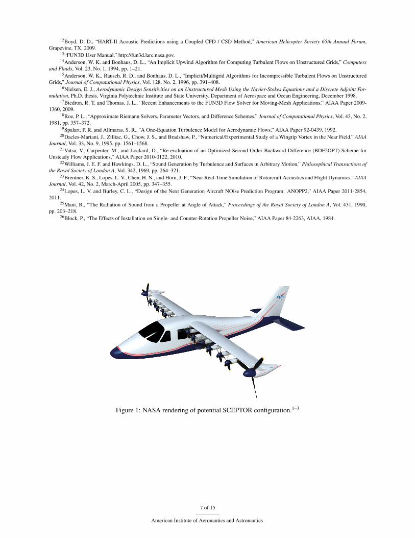
Over the past several years, the use of electric propulsion technologies within aircraft design has received increasedattention. The characteristics of electric propulsion systems open up new areas of the aircraft design space, suchas the use of distributed electric propulsion (DEP). In this approach, electric motors are placed in many differentlocations to achieve increased efficiency through integration of the propulsion system with the airframe. Under aproject called Scalable Convergent Electric Propulsion Technology Operations Research (SCEPTOR),1–3 NASA isdesigning a flight demonstrator aircraft similar to that shown in Figure 1. The configuration employs many “high-liftpropellers" distributed upstream of the wing leading edge and two cruise propellers (one at each wingtip). The high-lift propellers are designed to increase the dynamic pressure over the sections of the wing in the propeller slipstreams,thereby increasing the total lift. As they are meant to act similarly to conventional high-lift devices, these propellersonly operate at low flight speeds. At higher flight speeds, the two cruise propellers provide all the propulsive thrust forthe aircraft and the high-lift propellers are folded and stowed against the nacelles to reduce drag.

As the high-lift propellers are operational at low flight speeds (take-off/approach flight conditions), the impact ofthe DEP configuration on the aircraft noise signature is also an important design consideration. This paper describesan initial study of the source noise produced by the isolated high-lift propellers and sets the stage for the predictionof installation effects. The baseline design is a propeller concept used in initial DEP testing4, 5 and is representativeof subsequent high-lift propeller designs. The propeller configuration and operating conditions of interest are firstpresented in Section II. This is followed by a discussion of the aerodynamic and acoustic prediction codes in SectionsIII and IV. Comparison of predicted results are then presented in Section V. Finally, concluding remarks regardingsome of the more significant results and further areas of interest are presented in Section VI.

II. Propeller Configuration

The high-lift propeller considered in this study is the five-bladed design by Stoll4, 5 shown in Figure 2. As men-tioned above, this propeller design has been used in previous DEP studies4, 5 and is representative of initial high-liftpropeller designs. In addition, the design is scheduled to be tested in the NASA Langley Low Speed AeroacousticWind Tunnel (LSAWT)6 and measured performance and acoustic data will be available for subsequent validation.The propeller diameter is D = 0.44 m (1.44 ft) and the baseline forward flight speed, Vf = 31.4 m/s (103.0 ft/s), andpropeller RPM (5866) chosen for this study correspond to takeoff conditions. Predictions are performed at angles ofattack, α , ranging from 0◦− 9◦ to investigate angle of attack effects. In preparation for comparison with measureddata, additional forward flight speeds and propeller RPM at α = 0◦ are also briefly considered.

The observer locations for acoustic predictions are shown in Figure 2. Sideline directivity is captured on an arcof radius 3.54 m (11.60 ft) centered on the propeller axis and propeller plane of rotation. Sideline angles, θ , rangingfrom 0◦− 180◦ are included, with θ = 0◦ pointing in the upstream (forward flight) direction and θ = 180◦ pointingin the downstream (aft) direction. A ring (radius 3.54 m (11.60 ft)) of observers centered on the propeller axis in thepropeller plane of rotation encompassing the full range of azimuthal angles (0◦ ≤ φ ≤ 360◦) is also included to studyangle of attack effects. Looking downstream (aft) into the propeller, 0 ≤ φ ≤ 180◦ represents the upper half of thepropeller disc and 180≤ φ ≤ 360◦ represents the lower half of the propeller disc.

III. Aerodynamic Predictions

Both a structured and unstructured computational fluid dynamics (CFD) code, as well as a blade element approachare used in this study to predict propeller aerodynamic performance and obtain blade loading information. These codesare described in detail in the cited references, so only background information on the various codes is provided herein.

2 of 15

American Institute of Aeronautics and Astronautics

A. Propeller Analysis System (PAS)

The NASA Aircraft Noise Prediction Program (ANOPP) Propeller Analysis System7, 8 is a set of computational mod-ules for predicting the aerodynamics, performance, and noise of propellers. Classical aerodynamic theory is used tofind the surface pressures and frictional stresses on the blade surfaces. Specifically, propeller blade geometry is givenin terms of blade surface coordinates derived from a Joukowski transform of the blade sections. Potential flow aroundthe blade sections is computed by Theodorsen’s method by using the Kutta condition to fix the circulation. Bladeboundary layers are computed by using the Holstein-Bohlen method in the laminar region and the TrucKenbrodtmethod in the turbulent region.

B. OVERFLOW 2 (OVF)

OVERFLOW 29–12 is a three-dimensional time-marching implicit Navier-Stokes code that uses structured overset gridsystems. Several different inviscid flux algorithms and implicit solution algorithms are included and the code hasoptions for thin layer or full viscous terms. A wide variety of boundary conditions are available, as well as algebraic,one-equation, and two-equation turbulence models. Low speed preconditioning is also available for several of theinviscid flux algorithms and solution algorithms in the code. The code also supports bodies in relative motion, andincludes both a six-degree-of-freedom (6- DOF) model and a grid assembly code.

C. FUN3D (F3D)

The FUN3D flow solver13–17 has an extensive list of options and solution mechanisms for spatial and temporal dis-cretizations on general static or dynamic mixed-element unstructured meshes that may or may not contain oversetmesh topologies. In the current study, the spatial discretization uses a finite-volume approach in which the dependentvariables are stored at the vertices of mixed element meshes. Inviscid fluxes at cell interfaces are computed by usingthe upwind scheme of Roe,18 and viscous fluxes are formed by using an approach that is equivalent to a central differ-ence Galerkin procedure. The eddy viscosity is modeled by using the one-equation approach of Spalart and Allmaras19

with the source term modification proposed by Dacles-Mariani et al.20 Scalable parallelization is achieved throughdomain decomposition and message-passing communication.

An approximate solution of the linear system of equations that is formed within each time step is obtained throughseveral iterations of a multicolor Gauss-Seidel point-iterative scheme. The turbulence model is integrated all the wayto the wall without the use of wall functions. The turbulence model is solved separately from the mean flow equationsat each time step with a time integration and a linear system solution scheme that is identical to that employed for themean flow equations.

A dual time-stepping algorithm with subiterations is used to converge the solution within each physical time-step. For these simulations, a maximum of 20 subiterations per time-step was used. However, a temporal errorcontroller was used to monitor the subiteration convergence history advancing to the next physical time-step when theflow residuals dropped below ten percent of the estimated temporal error. A variety of time marching schemes areavailable in FUN3D, including a second-order backward-differencing formulation (BDF2), and an optimized secondorder backward differencing formulation (BDF2OPT). The BDF2OPT scheme21 was chosen for the current applicationas it produces lower truncation error compared to the standard BDF2 scheme at nominally the same computationalcost but with slightly increased memory usage.

IV. Acoustic Predictions

The acoustic prediction methods used in this study are based on the FW-H equation,22 which is a rearrangement ofthe exact continuity and Navier-Stokes equations into a wave equation for the density with a nonlinear forcing term.Through the application of generalized functions and a Green’s function technique, the solution to the equation canbe reduced to a surface and a volume integral, but the solution is often well approximated by the surface integralalone. The volume integral includes physical effects such as refraction and nonlinear steepening. When these effectsare small, the FW-H surface can coincide with the solid body generating the unsteady flow. This is often referred toas an impermeable data surface. When effects such as refraction are important, the FW-H surface can be pushed outinto the flow to encompass important flow gradients. In this case, the data surface is referred to as being permeable(also, penetrable or porous). Hence, the time history of the density, which is directly related to the pressure in thefar-field, can be obtained at locations far from the body from a surface integral that is either close to or on the actual

3 of 15

American Institute of Aeronautics and Astronautics

body. For permeable surfaces that are off the body, the time histories of all the flow variables are needed, but no spatialderivatives are explicitly required. For surfaces coinciding with the body, only the pressure time history is needed.

The PSU-WOPWOP (PSW) code23 and the F1A module of NASA’s second generation Aircraft NOise PredictionProgram (ANOPP2),24 both implementing Farassat’s retarded-time formulation 1A of the FW-H equation, are used tocalculate the propeller source noise. Both the solvers were used for the acoustic predictions at select conditions andthe two codes provided nearly identical results. Therefore, only a single set of results based on the PSW predictionsare presented and may be considered indicative of both acoustic prediction codes.

All acoustic predictions are based on impermeable data surfaces. In specifying the geometry and loading valuesfor the acoustic data surfaces, the information may be considered ‘constant’, ‘periodic’, or ‘aperiodic’. Informationspecified as ‘constant’ is assumed to remain unchanged for all source times. In terms of geometry, this means that theblade shapes remain unchanged as they rotate. For loading specification, the surface pressure values would remainunchanged as the blades rotate (as would be the case if the mean loading values were specified). For ‘periodic’ data,values are taken to change as a function of azimuthal angle. Finally, for ‘aperiodic’ data, values are taken to changearbitrarily as a function of time. The propeller blades are assumed rigid, with shapes taken to be the same at all speeds.Therefore, within the acoustic calculations, the geometry of the acoustic data surfaces could be considered ‘constant’and rotating at the specified RPM. This meant that surface geometry for only a single CFD time step would be neededas input. Alternatively, the data surfaces could be specified as ‘periodic’ and the geometry for all time steps would beneeded. Predictions were performed using both approaches to verify input specification and, as expected, essentiallyidentical results were obtained. Therefore, the acoustic data surface geometry is specified as ‘constant’ in subsequentpredictions due to the reduction in input file size. Conversely, the surface pressure loading is taken to be ‘periodic’ (i.e.,changing as a function of azimuthal angle and repeating on a once-per-revolution basis). Specifically, time dependentsurface pressure loading values for one full rotor revolution are extracted from the aerodynamic predictions solutions(after suitable convergence was reached for the CFD approaches) and used as input. For the cases utilizing the F3Dand OVF loading information, acoustic predictions are based on CFD values at 1.0◦ azimuthal resolution. However,due to issues with the Propeller Loading Module (PLD) of PAS, acoustic prediction utilizing the PAS loading arebased on information at 5.0◦ azimuthal resolution. More specifically, specification of 361 azimuthal angles in the PASinput generated an error condition indicating insufficient dynamic storage in the Propeller Loading Module (PLD).Therefore, the number of azimuthal angles was reduced to alleviate this issue. Acoustic results for α 6= 0◦ using thePAS loading are therefore expected to have reduced resolution for the higher harmonics of the blade passage frequency(BPF). This is an issue for future investigation regarding increased PAS azimuthal resolution, as well as the effects ofdecreased CFD azimuthal resolution on acoustic predictions.

V. Results and Discussion

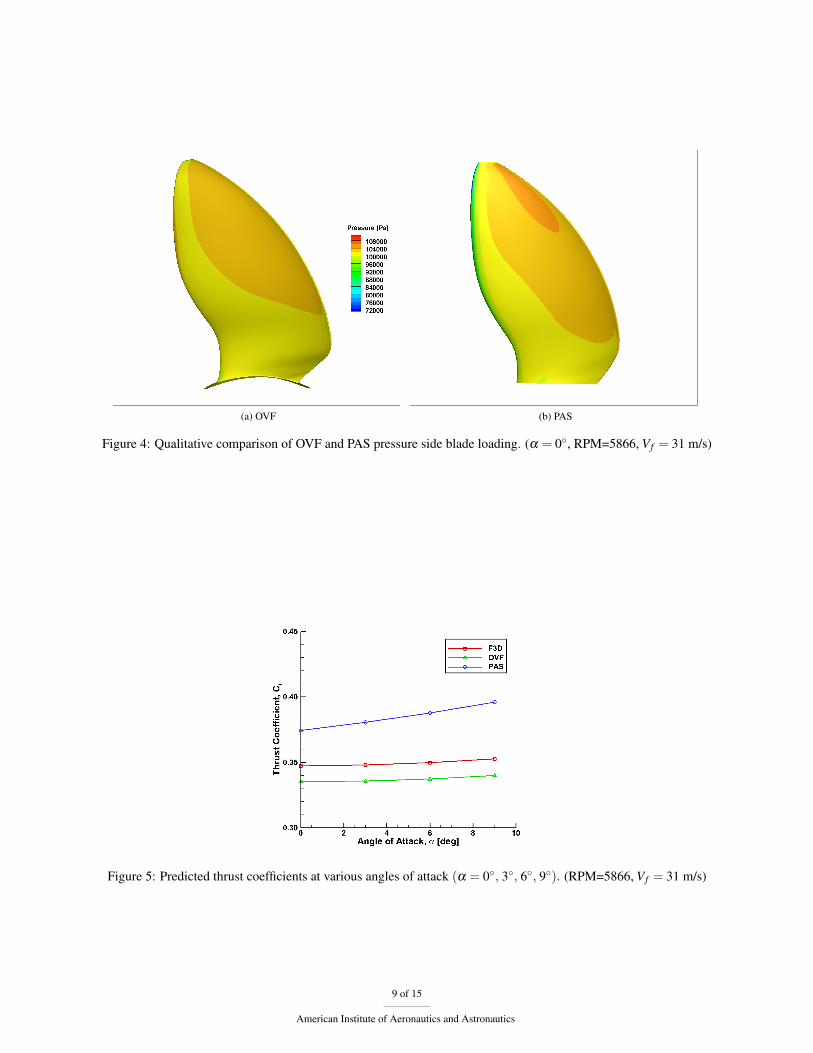
Aerodynamic and acoustic results are first presented for the cases related to nominal takeoff conditions (Vf =31.4 m/s (103.0 ft/s), RPM 5866). In all cases, the blade angles are kept constant. However, for the baseline case, theblade angle used in the PAS predictions was iterated upon until predicted thrust levels closely matched the averagebetween the F3D and OVF values. The result was a PAS blade angle that is approximately 5◦ less than that usedin the CFD predictions. Qualitative comparison of the OVF and PAS blade loads for the α = 0◦ case are shown inFigures 3-4. In addition to the differences in blade loading, these figure illustrate the geometrical differences relatedto the various aerodynamic prediction methodologies. Whereas the OVF and F3D blade geometries include the fullroot and tip regions, the PAS blade geometry has truncated root and tip regions due to the input requirements of theblade element approach. Despite these differences, the PAS results appear to capture the overall pressure distributionfairly well. This is further indicated by comparisons of the thrust coefficients in Figure 5 and overall thrust levels inTable 1. All of the predictions show a relative increase in thrust as the angle of attack is increased, with the PAS resultsshowing a slightly larger increase at α = 9◦.

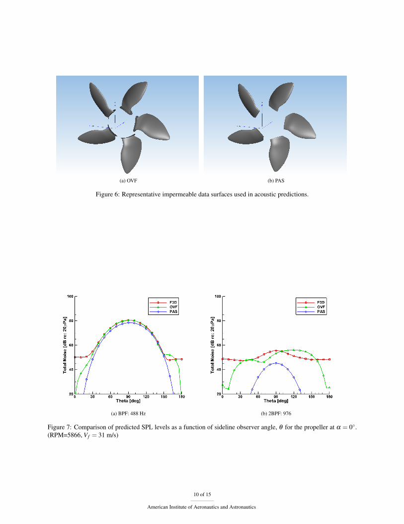
Acoustic predictions are obtained at locations corresponding to the observer arrangement shown in Figure 2. Asseen in Figure 6, only the rotor blade surfaces are included for which the required surface pressure values are providedby the aforementioned aerodynamic predictions. In addition to the blade surfaces, the OVF data surfaces contain aportion of the collar grids for each blade. The collar grids are necessary for the aerodynamic predictions and theinclusion of the small portion of the nacelle surface is assumed to have a negligible effect on the acoustic results.As mentioned above, the PAS data surfaces include truncated root and tip regions, which may affect acoustic results,particularly due to tip loading. While the separate thickness (monopole) and loading (dipole) acoustic contributionsare obtained in the predictions, only the total values are presented. In an attempt to cover a range of possible metricsfor prediction assessment, comparisons include the directivity for the dominant BPF tone, tonal amplitudes at BPF

4 of 15

American Institute of Aeronautics and Astronautics

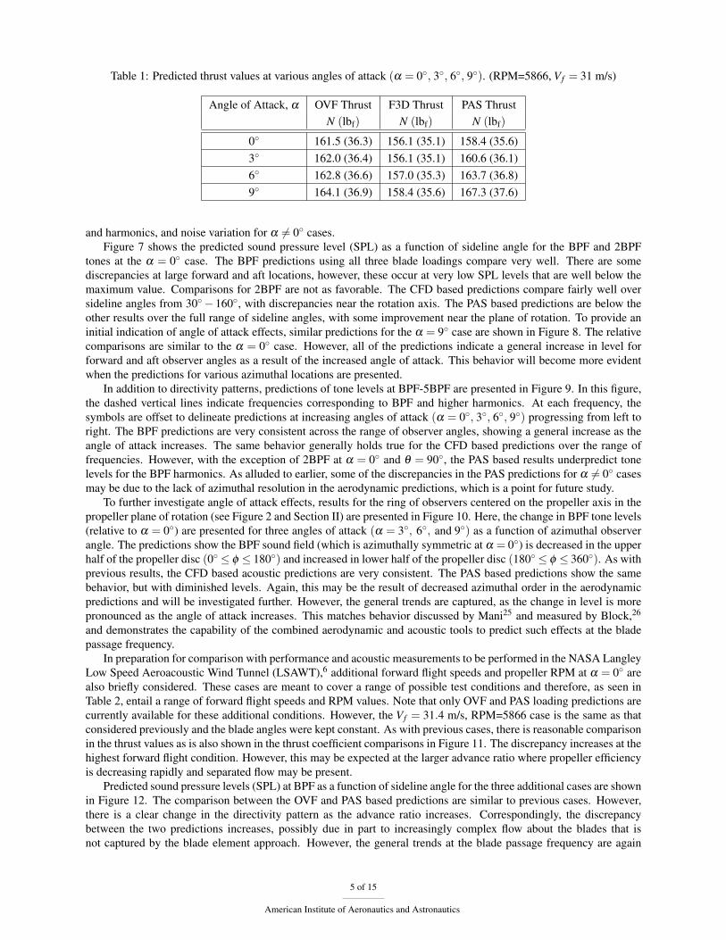
Table 1: Predicted thrust values at various angles of attack (α = 0◦, 3◦, 6◦, 9◦). (RPM=5866, Vf = 31 m/s)

Angle of Attack, α OVF Thrust F3D Thrust PAS ThrustN (lbf) N (lbf) N (lbf)

0◦ 161.5 (36.3) 156.1 (35.1) 158.4 (35.6)3◦ 162.0 (36.4) 156.1 (35.1) 160.6 (36.1)6◦ 162.8 (36.6) 157.0 (35.3) 163.7 (36.8)9◦ 164.1 (36.9) 158.4 (35.6) 167.3 (37.6)

and harmonics, and noise variation for α 6= 0◦ cases.Figure 7 shows the predicted sound pressure level (SPL) as a function of sideline angle for the BPF and 2BPF

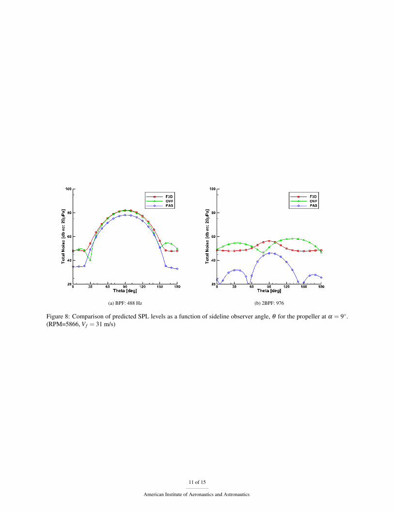
tones at the α = 0◦ case. The BPF predictions using all three blade loadings compare very well. There are somediscrepancies at large forward and aft locations, however, these occur at very low SPL levels that are well below themaximum value. Comparisons for 2BPF are not as favorable. The CFD based predictions compare fairly well oversideline angles from 30◦− 160◦, with discrepancies near the rotation axis. The PAS based predictions are below theother results over the full range of sideline angles, with some improvement near the plane of rotation. To provide aninitial indication of angle of attack effects, similar predictions for the α = 9◦ case are shown in Figure 8. The relativecomparisons are similar to the α = 0◦ case. However, all of the predictions indicate a general increase in level forforward and aft observer angles as a result of the increased angle of attack. This behavior will become more evidentwhen the predictions for various azimuthal locations are presented.

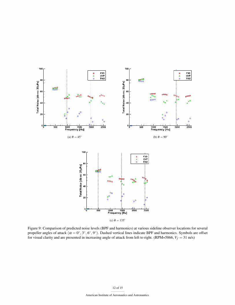
In addition to directivity patterns, predictions of tone levels at BPF-5BPF are presented in Figure 9. In this figure,the dashed vertical lines indicate frequencies corresponding to BPF and higher harmonics. At each frequency, thesymbols are offset to delineate predictions at increasing angles of attack (α = 0◦, 3◦, 6◦, 9◦) progressing from left toright. The BPF predictions are very consistent across the range of observer angles, showing a general increase as theangle of attack increases. The same behavior generally holds true for the CFD based predictions over the range offrequencies. However, with the exception of 2BPF at α = 0◦ and θ = 90◦, the PAS based results underpredict tonelevels for the BPF harmonics. As alluded to earlier, some of the discrepancies in the PAS predictions for α 6= 0◦ casesmay be due to the lack of azimuthal resolution in the aerodynamic predictions, which is a point for future study.

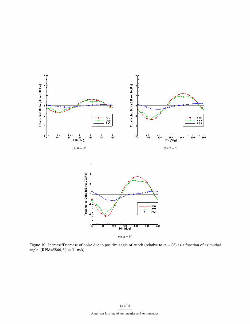
To further investigate angle of attack effects, results for the ring of observers centered on the propeller axis in thepropeller plane of rotation (see Figure 2 and Section II) are presented in Figure 10. Here, the change in BPF tone levels(relative to α = 0◦) are presented for three angles of attack (α = 3◦, 6◦, and 9◦) as a function of azimuthal observerangle. The predictions show the BPF sound field (which is azimuthally symmetric at α = 0◦) is decreased in the upperhalf of the propeller disc (0◦ ≤ φ ≤ 180◦) and increased in lower half of the propeller disc (180◦ ≤ φ ≤ 360◦). As withprevious results, the CFD based acoustic predictions are very consistent. The PAS based predictions show the samebehavior, but with diminished levels. Again, this may be the result of decreased azimuthal order in the aerodynamicpredictions and will be investigated further. However, the general trends are captured, as the change in level is morepronounced as the angle of attack increases. This matches behavior discussed by Mani25 and measured by Block,26

and demonstrates the capability of the combined aerodynamic and acoustic tools to predict such effects at the bladepassage frequency.

In preparation for comparison with performance and acoustic measurements to be performed in the NASA LangleyLow Speed Aeroacoustic Wind Tunnel (LSAWT),6 additional forward flight speeds and propeller RPM at α = 0◦ arealso briefly considered. These cases are meant to cover a range of possible test conditions and therefore, as seen inTable 2, entail a range of forward flight speeds and RPM values. Note that only OVF and PAS loading predictions arecurrently available for these additional conditions. However, the Vf = 31.4 m/s, RPM=5866 case is the same as thatconsidered previously and the blade angles were kept constant. As with previous cases, there is reasonable comparisonin the thrust values as is also shown in the thrust coefficient comparisons in Figure 11. The discrepancy increases at thehighest forward flight condition. However, this may be expected at the larger advance ratio where propeller efficiencyis decreasing rapidly and separated flow may be present.

Predicted sound pressure levels (SPL) at BPF as a function of sideline angle for the three additional cases are shownin Figure 12. The comparison between the OVF and PAS based predictions are similar to previous cases. However,there is a clear change in the directivity pattern as the advance ratio increases. Correspondingly, the discrepancybetween the two predictions increases, possibly due in part to increasingly complex flow about the blades that isnot captured by the blade element approach. However, the general trends at the blade passage frequency are again

5 of 15

American Institute of Aeronautics and Astronautics

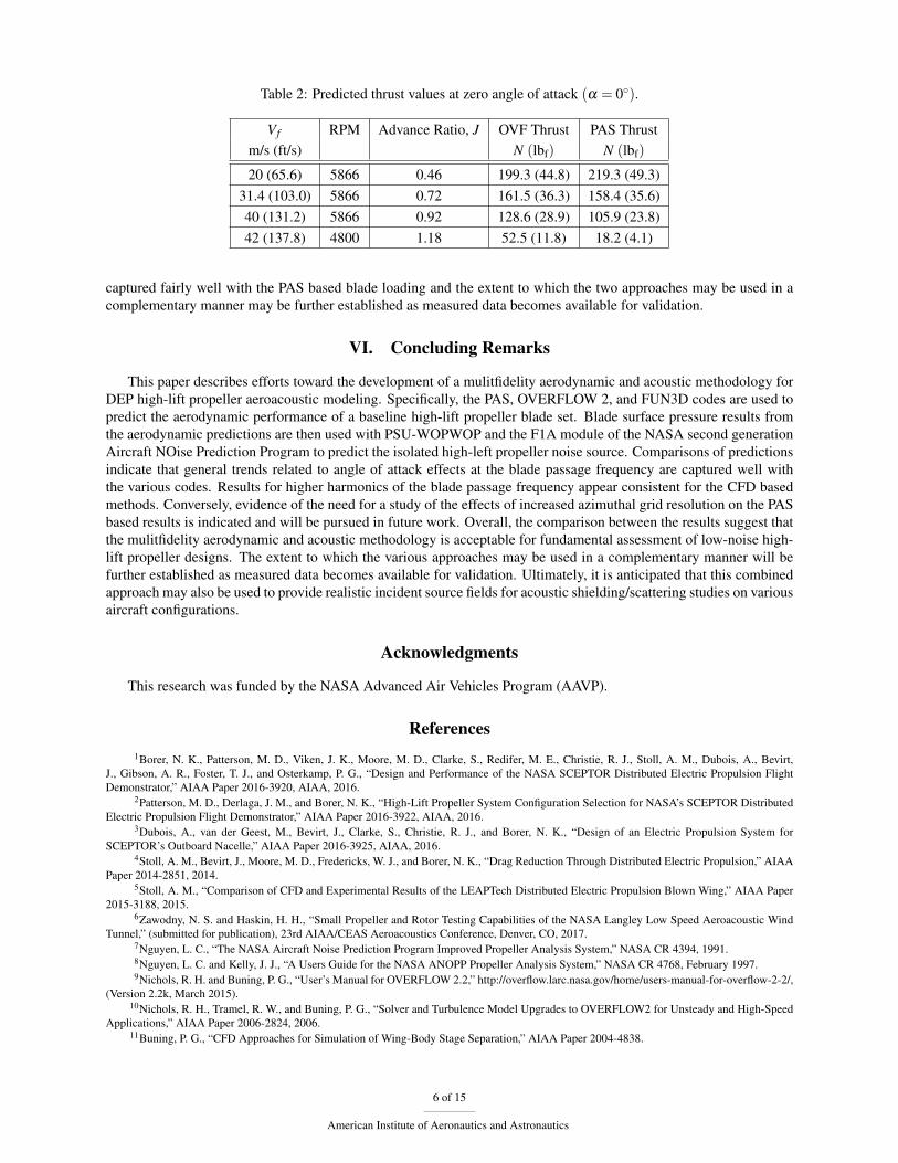
Table 2: Predicted thrust values at zero angle of attack (α = 0◦).

Vf RPM Advance Ratio, J OVF Thrust PAS Thrustm/s (ft/s) N (lbf) N (lbf)

20 (65.6) 5866 0.46 199.3 (44.8) 219.3 (49.3)31.4 (103.0) 5866 0.72 161.5 (36.3) 158.4 (35.6)40 (131.2) 5866 0.92 128.6 (28.9) 105.9 (23.8)42 (137.8) 4800 1.18 52.5 (11.8) 18.2 (4.1)

captured fairly well with the PAS based blade loading and the extent to which the two approaches may be used in acomplementary manner may be further established as measured data becomes available for validation.

VI. Concluding Remarks

This paper describes efforts toward the development of a mulitfidelity aerodynamic and acoustic methodology forDEP high-lift propeller aeroacoustic modeling. Specifically, the PAS, OVERFLOW 2, and FUN3D codes are used topredict the aerodynamic performance of a baseline high-lift propeller blade set. Blade surface pressure results fromthe aerodynamic predictions are then used with PSU-WOPWOP and the F1A module of the NASA second generationAircraft NOise Prediction Program to predict the isolated high-left propeller noise source. Comparisons of predictionsindicate that general trends related to angle of attack effects at the blade passage frequency are captured well withthe various codes. Results for higher harmonics of the blade passage frequency appear consistent for the CFD basedmethods. Conversely, evidence of the need for a study of the effects of increased azimuthal grid resolution on the PASbased results is indicated and will be pursued in future work. Overall, the comparison between the results suggest thatthe mulitfidelity aerodynamic and acoustic methodology is acceptable for fundamental assessment of low-noise high-lift propeller designs. The extent to which the various approaches may be used in a complementary manner will befurther established as measured data becomes available for validation. Ultimately, it is anticipated that this combinedapproach may also be used to provide realistic incident source fields for acoustic shielding/scattering studies on variousaircraft configurations.

Acknowledgments

This research was funded by the NASA Advanced Air Vehicles Program (AAVP).

References1Borer, N. K., Patterson, M. D., Viken, J. K., Moore, M. D., Clarke, S., Redifer, M. E., Christie, R. J., Stoll, A. M., Dubois, A., Bevirt,

J., Gibson, A. R., Foster, T. J., and Osterkamp, P. G., “Design and Performance of the NASA SCEPTOR Distributed Electric Propulsion FlightDemonstrator,” AIAA Paper 2016-3920, AIAA, 2016.

2Patterson, M. D., Derlaga, J. M., and Borer, N. K., “High-Lift Propeller System Configuration Selection for NASA’s SCEPTOR DistributedElectric Propulsion Flight Demonstrator,” AIAA Paper 2016-3922, AIAA, 2016.

3Dubois, A., van der Geest, M., Bevirt, J., Clarke, S., Christie, R. J., and Borer, N. K., “Design of an Electric Propulsion System forSCEPTOR’s Outboard Nacelle,” AIAA Paper 2016-3925, AIAA, 2016.

4Stoll, A. M., Bevirt, J., Moore, M. D., Fredericks, W. J., and Borer, N. K., “Drag Reduction Through Distributed Electric Propulsion,” AIAAPaper 2014-2851, 2014.

5Stoll, A. M., “Comparison of CFD and Experimental Results of the LEAPTech Distributed Electric Propulsion Blown Wing,” AIAA Paper2015-3188, 2015.

6Zawodny, N. S. and Haskin, H. H., “Small Propeller and Rotor Testing Capabilities of the NASA Langley Low Speed Aeroacoustic WindTunnel,” (submitted for publication), 23rd AIAA/CEAS Aeroacoustics Conference, Denver, CO, 2017.

7Nguyen, L. C., “The NASA Aircraft Noise Prediction Program Improved Propeller Analysis System,” NASA CR 4394, 1991.8Nguyen, L. C. and Kelly, J. J., “A Users Guide for the NASA ANOPP Propeller Analysis System,” NASA CR 4768, February 1997.9Nichols, R. H. and Buning, P. G., “User’s Manual for OVERFLOW 2.2,” http://overflow.larc.nasa.gov/home/users-manual-for-overflow-2-2/,

(Version 2.2k, March 2015).10Nichols, R. H., Tramel, R. W., and Buning, P. G., “Solver and Turbulence Model Upgrades to OVERFLOW2 for Unsteady and High-Speed

Applications,” AIAA Paper 2006-2824, 2006.11Buning, P. G., “CFD Approaches for Simulation of Wing-Body Stage Separation,” AIAA Paper 2004-4838.

6 of 15

American Institute of Aeronautics and Astronautics

12Boyd, D. D., “HART-II Acoustic Predictions using a Coupled CFD / CSD Method,” American Helicopter Society 65th Annual Forum,Grapevine, TX, 2009.

13“FUN3D User Manual,” http://fun3d.larc.nasa.gov.14Anderson, W. K. and Bonhaus, D. L., “An Implicit Upwind Algorithm for Computing Turbulent Flows on Unstructured Grids,” Computers

and Fluids, Vol. 23, No. 1, 1994, pp. 1–21.15Anderson, W. K., Rausch, R. D., and Bonhaus, D. L., “Implicit/Multigrid Algorithms for Incompressible Turbulent Flows on Unstructured

Grids,” Journal of Computational Physics, Vol. 128, No. 2, 1996, pp. 391–408.16Nielsen, E. J., Aerodynamic Design Sensitivities on an Unstructured Mesh Using the Navier-Stokes Equations and a Discrete Adjoint For-

mulation, Ph.D. thesis, Virginia Polytechnic Institute and State University, Department of Aerospace and Ocean Engineering, December 1998.17Biedron, R. T. and Thomas, J. L., “Recent Enhancements to the FUN3D Flow Solver for Moving-Mesh Applications,” AIAA Paper 2009-

1360, 2009.18Roe, P. L., “Approximate Riemann Solvers, Parameter Vectors, and Difference Schemes,” Journal of Computational Physics, Vol. 43, No. 2,

1981, pp. 357–372.19Spalart, P. R. and Allmaras, S. R., “A One-Equation Turbulence Model for Aerodynamic Flows,” AIAA Paper 92-0439, 1992.20Dacles-Mariani, J., Zilliac, G., Chow, J. S., and Bradshaw, P., “Numerical/Experimental Study of a Wingtip Vortex in the Near Field,” AIAA

Journal, Vol. 33, No. 9, 1995, pp. 1561–1568.21Vatsa, V., Carpenter, M., and Lockard, D., “Re-evaluation of an Optimized Second Order Backward Difference (BDF2OPT) Scheme for

Unsteady Flow Applications,” AIAA Paper 2010-0122, 2010.22Williams, J. E. F. and Hawkings, D. L., “Sound Generation by Turbulence and Surfaces in Arbitrary Motion,” Philosophical Transactions of

the Royal Society of London A, Vol. 342, 1969, pp. 264–321.23Brentner, K. S., Lopes, L. V., Chen, H. N., and Horn, J. F., “Near Real-Time Simulation of Rotorcraft Acoustics and Flight Dynamics,” AIAA

Journal, Vol. 42, No. 2, March-April 2005, pp. 347–355.24Lopes, L. V. and Burley, C. L., “Design of the Next Generation Aircraft NOise Prediction Program: ANOPP2,” AIAA Paper 2011-2854,

2011.25Mani, R., “The Radiation of Sound from a Propeller at Angle of Attack,” Proceedings of the Royal Society of London A, Vol. 431, 1990,

pp. 203–218.26Block, P., “The Effects of Installation on Single- and Counter-Rotation Propeller Noise,” AIAA Paper 84-2263, AIAA, 1984.

Figure 1: NASA rendering of potential SCEPTOR configuration.1–3

7 of 15

American Institute of Aeronautics and Astronautics

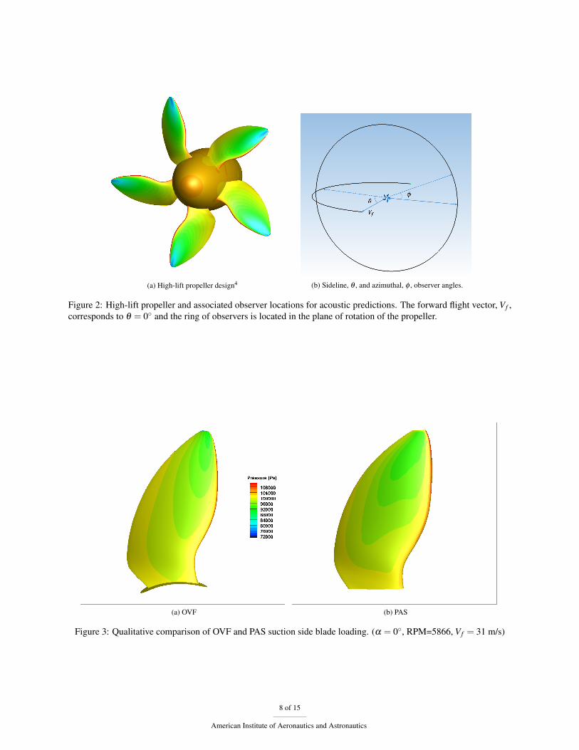
(a) High-lift propeller design4 (b) Sideline, θ , and azimuthal, φ , observer angles.

Figure 2: High-lift propeller and associated observer locations for acoustic predictions. The forward flight vector, Vf ,corresponds to θ = 0◦ and the ring of observers is located in the plane of rotation of the propeller.

(a) OVF (b) PAS

Figure 3: Qualitative comparison of OVF and PAS suction side blade loading. (α = 0◦, RPM=5866, Vf = 31 m/s)

8 of 15

American Institute of Aeronautics and Astronautics

(a) OVF (b) PAS

Figure 4: Qualitative comparison of OVF and PAS pressure side blade loading. (α = 0◦, RPM=5866, Vf = 31 m/s)

Figure 5: Predicted thrust coefficients at various angles of attack (α = 0◦, 3◦, 6◦, 9◦). (RPM=5866, Vf = 31 m/s)

9 of 15

American Institute of Aeronautics and Astronautics

(a) OVF (b) PAS

Figure 6: Representative impermeable data surfaces used in acoustic predictions.

(a) BPF: 488 Hz (b) 2BPF: 976

Figure 7: Comparison of predicted SPL levels as a function of sideline observer angle, θ for the propeller at α = 0◦.(RPM=5866, Vf = 31 m/s)

10 of 15

American Institute of Aeronautics and Astronautics

(a) BPF: 488 Hz (b) 2BPF: 976

Figure 8: Comparison of predicted SPL levels as a function of sideline observer angle, θ for the propeller at α = 9◦.(RPM=5866, Vf = 31 m/s)

11 of 15

American Institute of Aeronautics and Astronautics

(a) θ = 45◦ (b) θ = 90◦

(c) θ = 135◦

Figure 9: Comparison of predicted noise levels (BPF and harmonics) at various sideline observer locations for severalpropeller angles of attack (α = 0◦, 3◦, 6◦, 9◦). Dashed vertical lines indicate BPF and harmonics. Symbols are offsetfor visual clarity and are presented in increasing angle of attack from left to right. (RPM=5866, Vf = 31 m/s)

12 of 15

American Institute of Aeronautics and Astronautics

(a) α = 3◦ (b) α = 6◦

(c) α = 9◦

Figure 10: Increase/Decrease of noise due to positive angle of attack (relative to α = 0◦) as a function of azimuthalangle. (RPM=5866, Vf = 31 m/s)

13 of 15

American Institute of Aeronautics and Astronautics

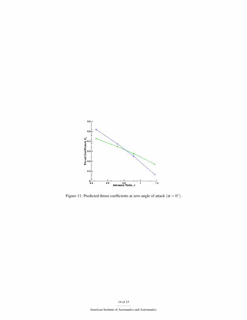
Figure 11: Predicted thrust coefficients at zero angle of attack (α = 0◦).

14 of 15

American Institute of Aeronautics and Astronautics

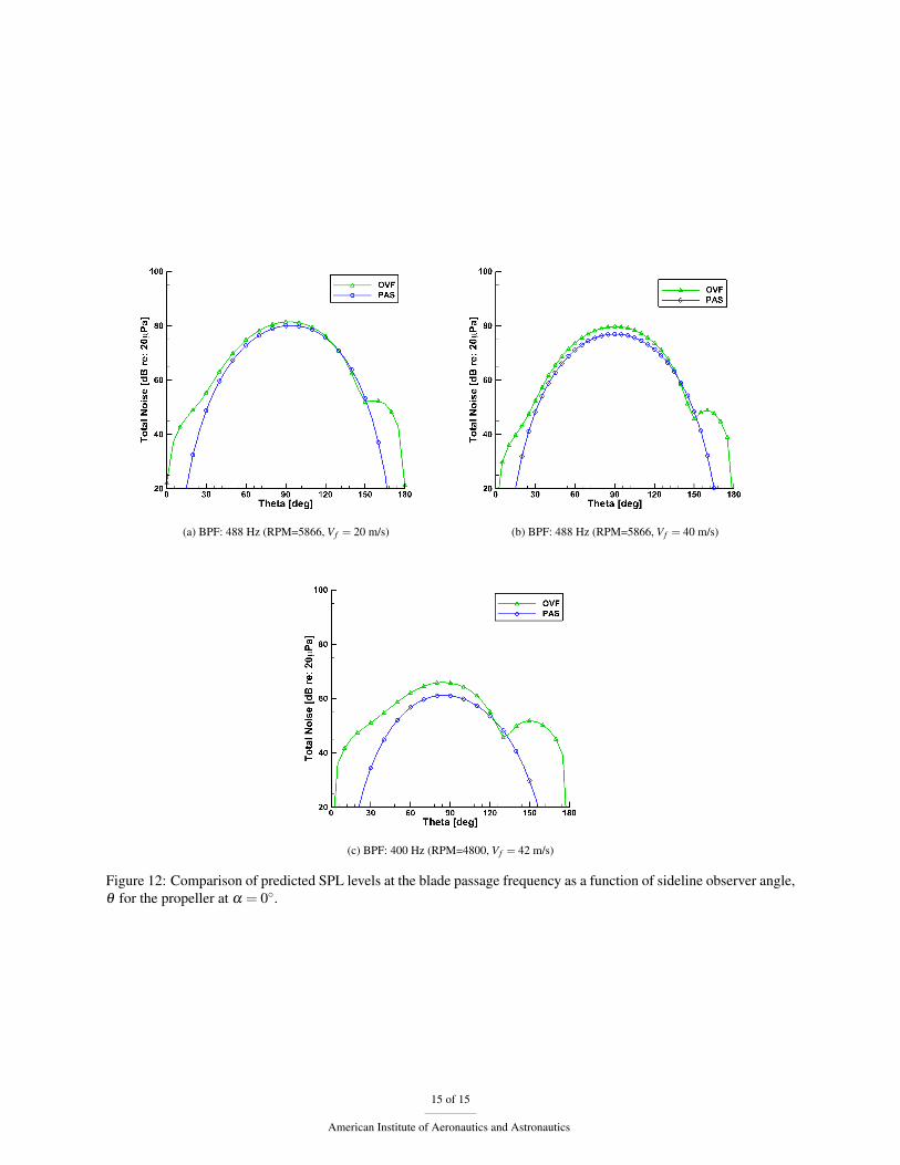
(a) BPF: 488 Hz (RPM=5866, Vf = 20 m/s) (b) BPF: 488 Hz (RPM=5866, Vf = 40 m/s)

(c) BPF: 400 Hz (RPM=4800, Vf = 42 m/s)

Figure 12: Comparison of predicted SPL levels at the blade passage frequency as a function of sideline observer angle,θ for the propeller at α = 0◦.

15 of 15

American Institute of Aeronautics and Astronautics