High-Lift OVERFLOW Analysis of the DLR-F11 Wind … · High-Lift OVERFLOW Analysis of the DLR-F11...

American Institute of Aeronautics and Astronautics

1 of 38

High-Lift OVERFLOW Analysis of the DLR-F11 Wind Tunnel Model

Thomas H. Pulliam* NASA Ames Research Center, Moffett Field, CA, 94035, USA

Anthony J. Sclafani† Boeing Research & Technology, Huntington Beach, CA, 92647, USA

In response to the 2nd AIAA CFD High Lift Prediction Workshop, the DLR-F11 wind tunnel model is analyzed using the Reynolds-averaged Navier-Stokes flow solver OVERFLOW. A series of overset grids for a bracket-off landing configuration is constructed and analyzed as part of a general grid refinement study. This high Reynolds number (15.1 million) analysis is done at multiple angles-of-attack to evaluate grid resolution effects at operational lift levels as well as near stall. A quadratic constitutive relation recently added to OVERFLOW for improved solution accuracy is utilized for side-of-body separation issues at low angles-of-attack and outboard wing separation at stall angles. The outboard wing separation occurs when the slat brackets are added to the landing configuration and is a source of discrepancy between the predictions and experimental data. A detailed flow field analysis is performed at low Reynolds number (1.35 million) after pressure tube bundles are added to the bracket-on medium grid system with the intent of better understanding bracket/bundle wake interaction with the wing’s boundary layer. Localized grid refinement behind each slat bracket and pressure tube bundle coupled with a time accurate analysis are exercised in an attempt to improve stall prediction capability. The results are inconclusive and suggest the simulation is missing a key element such as boundary layer transition. The computed lift curve is under-predicted through the linear range and over-predicted near stall, and the solution from the most complete configuration analyzed shows outboard wing separation occurring behind slat bracket 6 where the experiment shows it behind bracket 5. These results are consistent with most other participants of this workshop.

Nomenclature AR = win g aspect ratio, b2/Sref N = number of grid points b = win g span QCR = quadratic constitutive relation CFD = computational fluid dynamics RN = Reynolds number CD = drag coefficient, Drag/(q Sref) RANS = Reynolds-averaged Navier-Stokes Cf = skin friction coefficient Sref = win g reference area CL = lift coefficient, Lift/(q Sref) X = x-coordinate location, streamwise CM = pitching moment coefficient , Moment/(q SrefCref) Y = y-coordinate location, spanwise CP = pressure coefficient, (P-P )/q = angle-of-attack cref = win g reference chord = win g sweep c = chord = taper ratio HiLiftPW = high lift prediction workshop = semi-span station, Y/(b/2) LE = leading edge

I. Introduction XPANDING the use of Computational Fluid Dynamics (CFD) in the design and analysis of modern t ransport aircraft is a growing interest among many who seek to minimize costs associated with development and

certification. Meaningful applications of CFD tools have the potential to reduce wind tunnel and flight test time as well as to enhance databases for certification purposes. The Drag Prediction Workshop1 has demonstrated that the cruise portion of the flight envelope can be accurately simulated on geometry characterized predominantly by * Research Scientist, AIAA Associate Fellow. † Aerodynamics Engineer, AIAA Senior Member.

E

https://ntrs.nasa.gov/search.jsp?R=20140017729 2018-09-06T14:04:43+00:00Z


2 of 38

attached flow. While there is still more work to do to improve predictive capabilities in this flow regime such as increasing geometric complexity with confidence, the global CFD community is expanding its assessment of current generation codes to include geometry and flight segments that prove challenging on a fundamental level. Examples of this growing effort include the Aeroelastic Prediction Workshop2 and the High Lift Prediction Workshop3,4. By evaluating state-of-the-art methods applied to a common test case, aircraft designers and code developers effectively collaborate on a shared goal of improving CFD technology so that it can be more widely used in a configuration development process.

The 2nd High Lift Prediction Workshop4 (HiLiftPW-2) was held on June 22-23, 2013 in San Diego, California. The basic objective of this workshop is to assess CFD methods using a high-lift configuration that is relevant to industry participants, challenging for grid generators and flow solvers and rich in publicly available data. As shown in the 1st High Lift Prediction Workshop3 (HiLiftPW-1), using well defined test cases, geometry and flow conditions allow for informative data comparisons that often highlight areas in need of attention. For example, the vast majority of HiLiftPW-1 participants found that accurately simulating the wingtip flow field was difficult due to complex three-dimensional characteristics of the tip geometry. The workshop organizing committee intended to repeat this type of data exchange on a geometry considered more relevant than the Trap Wing given its relatively low aspect ratio and flat-sided body. The DLR-F11 wind tunnel model was selected as the test case for HiLiftPW-2 because it met the basic requirements for data availability and geometric relevancy. This paper summarizes structured overset grid results from an OVERFLOW study on the DLR-F11 high-lift wind tunnel model. This study was a collaborative effort between the Boeing and NASA authors where all HiLiftPW-2 test cases associated with the F11 were completed. The traditional data comparisons are made in this paper with force, moment, pressure, surface streamline and off-body velocity profiles discussed as a function of flow condition (i.e., angle-of-attack and Reynolds number) and grid density. Special attention is given to unique aspects of this work that include the effect of a Quadratic Constitutive Relation (QCR), extreme grid refinement behind slat brackets and time accurate simulations.

II. F11 Geometry and Test Data The test case geometry selected for HiLiftPW-2 is the DLR-F11 three-element wind tunnel model5 shown in

Figure 1. This geometry is considered representative of a modern transport configuration in terms of basic high -lift architecture, wing planform (e.g., sweep, taper and aspect ratio) and fuselage size/shape which includes a representative wing-body fairing. Multiple arrangements of the high-lift elements were tested but only one is used for the workshop which consists of a full-span leading-edge slat, a main wing element and a full-span trailing edge Fowler-motion flap. The rigging of the slat and flap are consistent with landing positions where the slat is deflected 26.5 degrees and the flap is deflected 32 degrees . Both the slat and flap are completely sealed to the fuselage. The flap side-of-body seal is facilitated by an additional surface as illustrated in Figure 2. Some basic reference quantities for the DLR-F11 wind tunnel model are provided in Table 1.

Table 1. DLR-F11 reference quantities.

Reference Area, Sref/2 419130 mm2 Aspect Ratio (AR), b2/Sref 9.353 Mean Aero Chord, cref 347.09 mm Quarter-Chord Sweep ( c/4) 30o Semi-Span, b/2 1400 mm Taper Ratio ( ), ctip/croot 0.3 Moment Reference, Xref 1428.9 mm Slat Chord Ratio, cslat/cwing 0.177 Moment Reference, Yref 0 mm Flap Chord Ratio, cflap/cwing 0.276 Moment Reference, Zref 41.61 mm Fuselage Length 3077 mm

The workshop test cases called for investigations to be performed on three levels of geometric fidelity. A

simplified configuration called “Config 2” was selected for a grid convergence study where the s lat brackets and flap fairings were not included. Effects of angle-of-attack and Reynolds number were studied on a more complex configuration called “Config 4” where the brackets and fairings were included. The most geometrically challenging configuration was Config 4 with simulated pressure tube bundles located next to each slat bracket. This geometry was labeled “Config 5.” A summary paper by Rudnick et al.5 documents additional information on the DLR-F11 wind tunnel model geometry. More details on Config 4 and 5 will be provided in the Results section of this paper.

The DLR-F11 semi-span model was tested in the Airbus Low-Speed Wind Tunnel (B-LSWT) and the European Transonic Wind Tunnel (ETW) at mean aerodynamic chord Reynolds numbers of 1.35 million and 15.1 million, respectively. The B-LSWT test was conducted at atmospheric conditions while the higher Reynolds number ETW


3 of 38

test was cryogenic. Force, moment and pressure data from both test campaigns were provided to workshop participants and formed the basis for the CFD test case flow conditions. Additional data from the B-LSWT test such as Particle Image Velocimetry (PIV) and oil surface flow visualization were also made available via the HiliftPW-2 website. A comprehensive overview of the wind tunnel data is available in the summary paper by Rudnick et al.5

III. Overset Grid Generation Overset grids were built for all of the F11 configurations defined as test cases for HiLiftPW-2. Grid generation

efforts were led by Tony Sclafani using both Boeing and NASA tools. Prior to releasing the overset grids for workshop participant use, Tom Pulliam and William Chan at NASA Ames Research Center examined them and provided feedback on various items such as topology and cell spacing. Improvements were made based on NASA’s input. In general, the same overset grid generation approach was followed that has been used for past Drag Prediction Workshop test cases6 and the “Trap Wing” test case from the 1st High Lift Prediction Workshop.7 This approach is outlined below with an emphasis on unique challenges associated with the F11 wind tunnel geometry as well as how “lessons learned” from previous workshops were applied.

A. Medium Grid The medium grid was built first using a proven high-lift grid generation strategy consistent with that used in the

1st High Lift Prediction Workshop.7 The same surface grid topology found in the Trap Wing grid system was applied to the F11 with standard collar grids joining lifting elements to the fuselage, trailing-edge cap grids defining the blunt base, and tip cap grids closing-off the tip geometry. Figure 3 gives a high-level overview of the surface grid layout with the various grid types marked. Note the dense regions of spacing in the span direction intended to provide comparable cell sizes in overlap regions as well as capture the interaction between brackets and downstream elements. This spanwise clustering is also shown in Figure 4 and is one of the lessons learned by the authors from the first high-lift workshop. That is, this higher grid resolution required for slat/flap bracket modeling had a significant impact on lift levels near stall for the Trap Wing wind tunnel model. In order to be consistent across all F11 test cases as well as with the Trap Wing grid approach, the spanwise clustering was applied to all configurations regardless of whether or not the brackets were actually modeled.

The overset grid topology shown in Figure 3 was constructed by first loading Initial Graphics Exchange Specification (IGES) files into a Boeing-developed program called Modular Aerodynamic Design Computational Analysis Process (MADCAP).8 MADCAP is a graphical user interface that drives multiple routines for structured and unstructured surface and volume grid generation. The F11 “Config 2” medium mesh was built manually in this environment following workshop gridding guidelines defined on the HiLiftPW-2 website9 which offer general suggestions on grid topology and point spacing. These guidelines were strictly adhered to for the F11 medium mesh and can be referenced to learn more about the grid such as stretching ratio. A significant effort was made to ensure that all surface grid points are a true representation of the geometry provided in the IGES file. The slat, wing and flap surfaces were modeled using a standard c-mesh topology where the wake sheet was defined using a potential flow solver set to an angle-of-attack of 10 degrees. The wake sheets are not shown in Figures 3 and 4 for clarity. The images in these figures do show how the c-mesh grids were broken into pieces in the span direction with overlap added for communication purposes. This was done in anticipation of file size limitations associated with the extra-fine grid which will be further discussed in the next sub-section.

Volume grid generation was accomplished using a script system10 developed at NASA which is intended to work with the Chimera Grid Tools (CGT).11 This script system offers a degree of automation to the overall process by defining boundary conditions for each grid, organizing components with a master configuration file, and driving the CGT programs with a master input file. A script tool called BuildVol generates volume grids where surface grids are run through one of two hyperbolic grid generators (HYPGEN12 and LEGRID) and Cartesian box grids are created using BOXGR. The final step in the grid generation process is to establish grid connectivity using PEGASUS513. Individual grid zones are connected by cutting holes where points fall inside geometry or where another grid is found to have better spacing. At grid and hole boundaries, PEGASUS5 creates interpolation stencils which are needed to pass information. After PEGASUS5 was run, a force and moment integration surface was created using another NASA CGT program called MIXSUR. This program eliminates grid overlap on the surface and connects neighboring zones with zipper grids comprised of triangles. MIXSUR produces a closed integration surface used to compute forces and moments.

The grid generation process outlined here was only followed for the “initial” medium mesh. A family of grids was then built for the convergence study using another tool set and a process established for past Drag Prediction


4 of 38

Workshop studies. This process resulted in a “final” medium mesh that was an integral part of an interleaved grid family.

B. Coarse, Fine, and Extra-Fine Grids The medium grid built using the tools described in the previous paragraphs was used as a starting point for a grid

family. As in past workshops, this family of overset grids was designed to be parametrically equivalent where a coarser mesh is a subset of the next denser mesh. A purpose-built program, developed at Boeing, redistributes points in an existing grid using a weighted-average cubic (WAC) interpolation routine. The user has control over how many grid points are added or taken away from the input mesh and whether surface breaks are preserved. The approach followed to define the grid family for the F11 test case is illustrated in Figure 5. The vertical dashed lines in this image show how there is a subset of points common to all four grid levels. Also note that the extra-fine (EF) and medium (M) grids have a 2-to-1 cell relationship as well as the fine (F) and coarse (C) grids. To achieve this relationship within the grid family, the WAC point redistribution tool was first applied to the volume grids of the initial medium mesh by doubling the number of cells in all three directions to create the extra-fine mesh. Since the surface definition was not preserved in this first step, the extra-fine grid was split apart by zone so that all surface abutting zones could be projected back to the loft definition. At this point in the process, the extra-fine grid was used to generate two coarser grids. First, every other point was removed from the extra-fine mesh to create the (final) medium mesh. This 2-to-1 cell relationship is shown in the blue lines of Figure 5 and highlighted in Table 2 by blue font.

Table 2. F11 overset grid family for Config 2.

Note that Table 2 compares the total number of grid points, not cells, which is why the ratio between extra-fine and medium is not exactly 23. The medium mesh generated by removing every other point from the extra-fine mesh was used as the final grid for the remainder of this study. In a practical sense, it is not any different from the initial medium mesh built using a more standard approach. However, it was extremely easy to create once the extra-fine grid was established so, in the spirit of consistency, it was used. The fine grid was built next in a similar manner as the medium grid. Instead of removing every other point from the extra-fine grid, a 4-to-3 cell ratio was maintained where the fine grid has three cells for every four cells in the extra-fine grid. This relationship is shown in Figure 5 as well as Table 2. Since the WAC interpolation routine relocated points in the fine grid, another projection step was required to ensure consistency in the surface definition across the overset family. The last step in the generation of the overset family was to create the coarse grid by removing every other point from the fine grid. This means the fine and coarse grids share the same 2-to-1 cell ratio as the extra-fine and medium grids. The two sets of 2-to-1 grid pairs were interleaved to form a family suitable for the HiLiftPW-2 convergence study.

As noted in Section III.A and shown in Figure 3, the slat/wing/flap grids were split in the span direction so the maximum record length in the extra-fine grid solution file would not be exceeded. The same procedure followed for the NASA Common Research Model grids in the 4th Drag Prediction Workshop6 was applied to the F11 grid. A maximum record length of 2,147,483,648 bytes was used to establish an upper bound on grid point count for a given zone in the largest grid. For the OVERFLOW solution file, 8 double-precision (64 bit or 8 byte) variables were assumed for each grid point. This means the solution file could contain 64 bytes of information at each point. Dividing the maximum record length of 2 gigabytes by 64 bytes/point gives an upper limit of 33.5 million points per zone. As a result, the slat grid was broken into three pieces, the wing was broken into four pieces, and the flap was broken into 2 pieces. The additional overlap from this partitioning together with the spanwise point clustering for slat brackets and flap fairings drove the overall point count up for all four grid levels. As noted in the HiLiftPW-2


5 of 38

summary paper4, the overset grid family had the greatest number of points for a given refinement level compared to all of the committee-supplied grids.

A series of surface grid images from the overset family are provided in Figures 6, 7 and 8 showing close-up views of the inboard slat/wing, inboard wing/flap and outboard slat/wing/flap upper surfaces, respectively. Figure 9 shows an off-body grid plane extracted from the coarse mesh near the wing’s trailing-edge break. This image, which is representative of the entire wing span, illustrates how the grid was manually refined to capture wakes from upstream elements as well as to increase resolution in shear layers such as the ones shedding off the slat lower trailing-edge and wing lower surface as it transitions to the flap cove. This off-body refinement is another reason why the overset grid family had the most number of points for a given level compared to other workshop committee supplied grids. For the coarse grid shown in Figure 9, minimum wall spacing was set to give a y+ of 1.0 based on a mean aerodynamic chord Reynolds number of 15.1 million. As the coarse grid was refined, the y+ value dropped below 1.0. Additional grid statistics and images will be discussed for the slat brackets, flap fairings and pressure tube bundles in the Results section of the paper.

IV. Flow Solver and Computing Platform OVERFLOW14 is a Reynolds Averaged Navier-Stokes (RANS) code widely used to compute subsonic,

transonic, and supersonic flow about complex configurations . The node-centered solver was specifically designed for structured overset grid systems like those built for HiLiftPW-2. OVERFLOW is capable of simulating many types of flow fields with options such as time accuracy, moving body and grid adaption with several choices for numerical scheme, boundary condition and turbulence model. The initial strategy the authors followed for HiLiftPW-2 was to simply use the approach that worked best for the Trap Wing test case in the first workshop. This means little effort was spent on investigating the effects of differencing scheme or turbulence model for the DLR-F11 prior to the workshop. The initial set of results obtained using a default setup raised many questions. Some of these questions were eventually addressed by exercising some of the options OVERFLOW has to offer. The solution restart capability was used to quantify the effect of initial conditions. A nonlinear stress model was applied to evaluate its effect on convergence characteristics. Finally, the code was run in time accurate mode to model flow field unsteadiness at high angles-of-attack.

OVERFLOW version 2.2f was used for the DLR-F11 analysis with an initial setup consisting of the full Navier-Stokes option (as opposed to thin-layer mode), Roe upwind differencing with third-order spatial accuracy for diffusion terms, Beam-Warming scalar pentadiagonal scheme for convection terms, the “noft2” version of the Spalart-Allmaras one-equation turbulence model15 with rotation and curvature corrections16 turned-on and multi-grid convergence acceleration. Other settings include low-Mach preconditioning and an exact wall distance calculation. Unless noted, all cases were run in a non-time accurate mode (e.g. full-multigrid, spatially varying time steps). Unsteady cases were run using dual time stepping, second order accuracy and every attempt was made to integrate to some form of convergence, either an asymptotic unsteady state or a converged mean state. Additional details on the various flow solver settings applied for this analysis, such as a nonlinear stress model, will be discussed throughout the Results section.

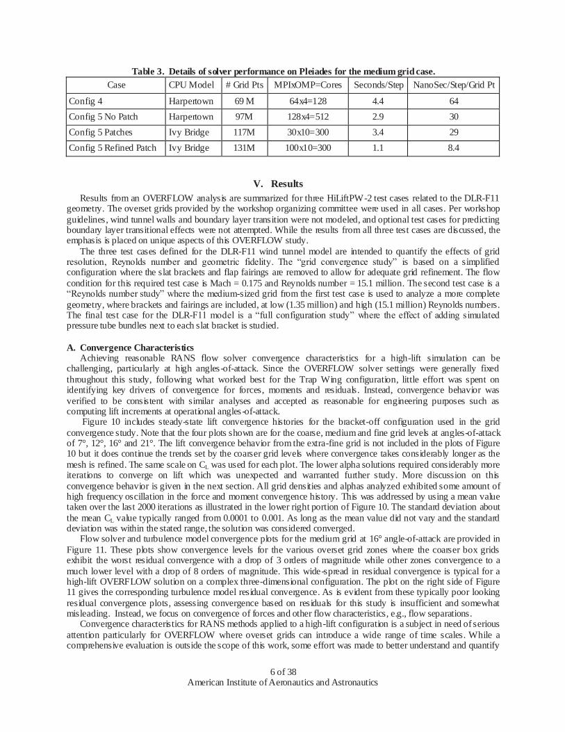
All cases were run in parallel using the Message Passing Interface (MPI) libraries and OpenMP on the NASA Pleiades supercomputer, which currently consists of 184,800 cores available on 11,176 compute nodes of mixed types. The strategy for selecting the number of cores for each grid size evolved over the course of time and the evolution of the Pleiades system. It was based on maintaining roughly 200,000-500,000 grid points per core, and in general at least 4 OpenMP threads were used, with up to 10 used on the larger grid systems. With this approach, the medium mesh reached full convergence on forces and moments in 10 hours running at a rate of 4.4 seconds per iteration on Harpertown nodes and about 3 hours of running at a rate of 1.1 seconds per iteration for the larger cases using Ivy-Bridge nodes. The larger grids required more wall clock time to converge due to s maller time scales. Table 3 shows a typical set of resource usages across the various cases. In this table, the word “Patch” is a reference to local grid refinement performed behind each slat bracket, “MPI” is number of MPI ranks and “OMP” is number of OpenMP threads. The unsteady cases discussed below required on the order of 10 times the running time when 10 dual-time step iterations are used per physical time step. Residual convergence characteristics will be discussed in the Results section.


6 of 38

Table 3. Details of solver performance on Pleiades for the medium grid case. Case CPU Model # Grid Pts MPIxOMP=Cores Seconds/Step NanoSec/Step/Grid Pt

Config 4 Harpertown 69 M 64x4=128 4.4 64 Config 5 No Patch Harpertown 97M 128x4=512 2.9 30 Config 5 Patches Ivy Bridge 117M 30x10=300 3.4 29 Config 5 Refined Patch Ivy Bridge 131M 100x10=300 1.1 8.4

V. Results Results from an OVERFLOW analysis are summarized for three HiLiftPW-2 test cases related to the DLR-F11

geometry. The overset grids provided by the workshop organizing committee were used in all cases. Per workshop guidelines, wind tunnel walls and boundary layer transition were not modeled, and optional test cases for predicting boundary layer transitional effects were not attempted. While the results from all three test cases are discussed, the emphasis is placed on unique aspects of this OVERFLOW study.

The three test cases defined for the DLR-F11 wind tunnel model are intended to quantify the effects of grid resolution, Reynolds number and geometric fidelity. The “grid convergence study” is based on a simplified configuration where the slat brackets and flap fairings are removed to allow for adequate grid refinement. The flow condition for this required test case is Mach = 0.175 and Reynolds number = 15.1 million. The second test case is a “Reynolds number study” where the medium-sized grid from the first test case is used to analyze a more complete geometry, where brackets and fairings are included, at low (1.35 million) and high (15.1 million) Reynolds numbers. The final test case for the DLR-F11 model is a “full configuration study” where the effect of adding simulated pressure tube bundles next to each slat bracket is studied.

A. Convergence Characteristics Achieving reasonable RANS flow solver convergence characteristics for a high-lift simulation can be

challenging, particularly at high angles-of-attack. Since the OVERFLOW solver settings were generally fixed throughout this study, following what worked best for the Trap Wing configuration, little effort was spent on identifying key drivers of convergence for forces, moments and residuals. Instead, convergence behavior was verified to be consistent with similar analyses and accepted as reasonable for engineering purposes such as computing lift increments at operational angles-of-attack.

Figure 10 includes steady-state lift convergence histories for the bracket-off configuration used in the grid convergence study. Note that the four plots shown are for the coarse, medium and fine grid levels at angles-of-attack of 7°, 12°, 16° and 21°. The lift convergence behavior from the extra-fine grid is not included in the plots of Figure 10 but it does continue the trends set by the coarser grid levels where convergence takes considerably longer as the mesh is refined. The same scale on CL was used for each plot. The lower alpha solutions required considerably more iterations to converge on lift which was unexpected and warranted further study. More discussion on this convergence behavior is given in the next section. All grid densities and alphas analyzed exhibited some amount of high frequency oscillation in the force and moment convergence history. This was addressed by using a mean value taken over the last 2000 iterations as illustrated in the lower right portion of Figure 10. The standard deviation about the mean CL value typically ranged from 0.0001 to 0.001. As long as the mean value did not vary and the standard deviation was within the stated range, the solution was considered converged.

Flow solver and turbulence model convergence plots for the medium grid at 16° angle-of-attack are provided in Figure 11. These plots show convergence levels for the various overset grid zones where the coarser box grids exhibit the worst residual convergence with a drop of 3 orders of magnitude while other zones convergence to a much lower level with a drop of 8 orders of magnitude. This wide-spread in residual convergence is typical for a high-lift OVERFLOW solution on a complex three-dimensional configuration. The plot on the right side of Figure 11 gives the corresponding turbulence model residual convergence. As is evident from these typically poor looking residual convergence plots, assessing convergence based on residuals for this study is insufficient and somewhat misleading. Instead, we focus on convergence of forces and other flow characteristics, e.g., flow separations.

Convergence characteristics for RANS methods applied to a high-lift configuration is a subject in need of serious attention particularly for OVERFLOW where overset grids can introduce a wide range of time scales. While a comprehensive evaluation is outside the scope of this work, some effort was made to better understand and quantify


7 of 38

convergence behavior for the DLR-F11 grid system by considering effects of a quadratic constitutive relation and time accuracy. The results of these side-studies are discussed in the following sections.

B. Test Case 1 – Grid Convergence Study The first test case for HiLiftPW-2 is a grid convergence study that all participants were required to complete.

The Drag Prediction Workshop (DPW) series has shown that a grid convergence study using Richardson extrapolation can yield valuable information regarding flow solver spatial accuracy order, level of discretization error and sensitivity of forces to grid resolution. It is accepted that application of Richardson extrapolation to a high-lift configuration may not be as fruitful as past cruise drag studies due to inherent flow field separation, but evaluating the effect of grid resolution may provide information not easily obtained using a single grid density. The flow condition used for the grid convergence study is based on the higher Reynolds number of 15.1 million and Mach 0.175. Solutions for two angles-of-attack, 7° and 16°, were to be evaluated for the bracket-off “Config 2” geometry. In addition to these two required angles, the overset grid family was used to evaluate grid refinement at alphas of 12°, 18.5°, 20°, 21° and 22.4°. Trends in lift, drag and pitching moment are summarized below with an emphasis on the effect of a nonlinear stress model recently implemented in OVERFLOW. As the grid convergence results are presented, it is important to remember that absolute levels of computed forces and moments are not expected to match test data due to the lack of brackets in the simulation.

Before the grid convergence study results are discussed, lift convergence history is more closely evaluated to better understand why so many iterations were required at lower angles -of-attack. The convergence plot for = 7° is shown in the upper-left portion of Figure 10. The medium mesh (red line) was run over 100,000 iterations before lift settled-in to a limit cycle oscillation where the mean value was not changing significantly. The coarse and fine grids exhibited similar convergence behavior at this angle-of-attack. The region of the flow field driving this slowly developing force convergence was identified by comparing solutions at iteration 9,971 and 103,500. Figure 12 includes a surface contour image colored by CL which is based on the difference in surface pressure computed at the two extreme iterations. This image clearly shows the largest variation on the surface was at the side-of-body in the region of the wing trailing-edge and flap. Figure 13 provides additional evidence that the solution in the wing-body juncture region was the primary difference between iteration 9,971 and 103,500. The red iso-surface in this figure represents the difference in stagnation pressure between the two flow solver iterations, and the surface streamline images show how side-of-body separation develops primarily in the juncture between the flap and fuselage. The discovery of slowly developing separation in a corner formed by two intersecting surfaces was disturbing given recent experience with similar flow physics on the cruise configurations of DPW where OVERFLOW was shown to over-predict the size of a side-of-body separation bubble compared to experimental data. In DPW-517, a newly developed quadratic constitutive relation (QCR) was successfully tested on the NASA Common Research Model (CRM) to address this over-prediction. The DLR-F11 test case was considered another good opportunity to test this new feature of the OVERFLOW flow solver.

As stated in Ref. 17, the idea of improving upon the eddy viscosity approximation by using a nonlinear stress term to model the Reynolds stresses directly was presented by Spalart18 who demonstrated that, by allowing for a more accurate anisotropic Reynolds-stress tensor via a rotation tensor, improved results are obtained for problems where turbulence-generated secondary flow structure is important. Spalart demonstrated the positive effect of a non-linear constitutive relation using a square duct test case. His results show a clear improvement in the four corners of the duct where computed skin friction was in better agreement with experiment compared to a linear, or Boussinesq, eddy viscosity model. A quadratic (i.e., nonlinear) constitutive relation (QCR), recently implemented in OVERFLOW, was turned-on for the bracket-off Config 2 overset grid family of Test Case 1. The effect on lift convergence is shown in Figure 14. The solution was restarted with QCR turned-on, and the lift coefficient at = 7° increased from 1.944 to 1.975. Based on the surface streamline images in Figure 14, the amount of separation computed in the juncture between the flap upper surface and fuselage was reduced after QCR was activated. This is the same trend seen in the CRM results from DPW-5.

The effect of grid resolution on computed lift coefficient is plotted in Figure 15 using Richardson extrapolation. In these plots, the horizontal axis data are the number of grid points raised to the -2/3 power so denser grids are represented by smaller values. The effect of QCR was quantified for multiple grid levels at angles-of-attack of 7°, 12° and 16°. At the lowest alpha of 7°, QCR increased lift for the coarse, medium and fine grids but had little effect for the extra-fine grid. Using QCR for the grid family at 12° and 16° produced more linear trends with refinement but it did not always result in a lift increase. The CL values shown in Figure 15 are plotted as a function of angle-of-attack in Figure 16 with wind tunnel data included for reference. The results with QCR are in better agreement with experiment through the linear portion of the lift curve where s lopes are consistent as opposed to the QCR-off data where results at lower angles-of-attack do not trend well. The data in Figure 16 also suggest that OVERFLOW over-


8 of 38

predicts the lift level at higher angles where stall was not predicted through 22.4° for both QCR-off and on. The effect of QCR-on stall prediction will be further explored in the next sub-section with the brackets included.

Computed drag variation with grid level is compared in Figure 17 for several angles-of-attack. With the drag scaled used, where a major tick represents 200 drag counts, there appears to be little difference between the coarse, medium and fine grid results. The 12° dataset is the only exception due to a jump in drag level between the medium and fine grid but this nonlinear trend is not present with QCR. Drag polar comparisons are provided in Figure 18 where the idealized induced drag, CL

2/( eAR) with the Oswald efficiency number (e) set to 1, is removed in order to plot the data on a tighter scale for detailed polar shape comparisons. This “idealized” drag comparison clearly shows how the OVERFLOW results do not agree well with the experimental data in terms of polar shape. There is a general trend with grid refinement where the increased resolution drives the answer in the direction of the measured data. By comparing the QCR-off (left side of Figure 18) and QCR-on (right side of Figure 18) polars, the conclusion can be made that QCR improves data consistency in terms of drag polar shape.

The pitching moment comparisons made in Figures 19 and 20 suggest the effect of QCR is significantly larger than its effect on lift and drag. Unlike the lift comparisons given in Figure 15, the pitching moment trends with grid refinement are not improved when QCR is activated. There is a break in the trend line for the 7° data set between the fine and extra-fine grid results, and the 16° trend is nonlinear between the medium and fine grids which is a feature of all the higher angles-of-attack. Pitching moment curves are compared in Figure 20 to evaluate the general shape and level relative to experimental data. OVERFLOW predicts a considerably more nose-down moment with no strong nose-up break as seen in the test data which suggests outboard separation or lack thereof in the CFD results .

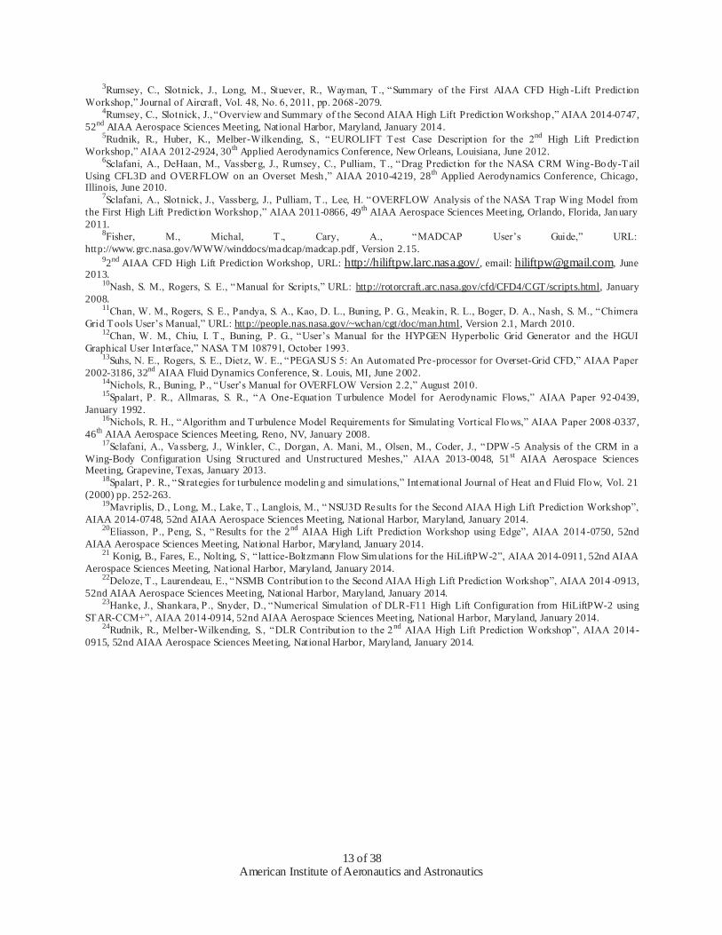
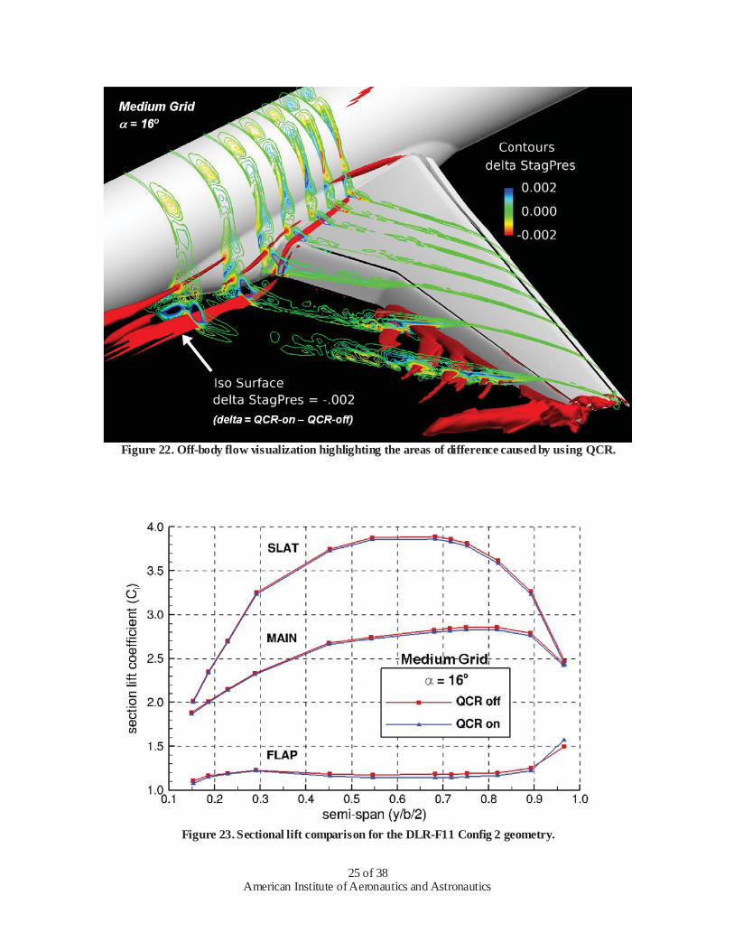
Surface flow visualization images are compared in Figure 21 to identify the source of the pitching moment shift caused by QCR at 16°. There is little difference seen in surface streamlines across the medium, fine and extra-fine grid levels, but there is a QCR effect visible at the side-of-body for a given grid. The QCR-on streamlines group together tighter where an off-body vortex interacts with the surface flow suggesting a stronger influence. Figure 22 is an image illustrating where QCR has the most significant effect on the off-body flow field. The contours in this image are defined as the difference in stagnation pressure between the QCR-on and QCR-off solutions. This differencing underscores the conclusion made from the surface streamline comparison in Figure 21 which is the side-of-body flow field is heavily influenced by QCR. Figure 22 also shows differences downstream of the mid-span flap region suggesting QCR’s effect is considerable in all areas of the field where strong rotational flow is predicted. In order to tie-in the surface and off-body flow changes with pitching moment, a spanload comparison is plotted in Figure 23 for the medium grid at 16° angle-of-attack. The changes in sectional loading shown in this plot are in-line with the flow visualization images with differences seen across the entire span of the flap. The change in flap loading likely drives the load changes on the slat and wing as shown in Figure 23.

The force and moment comparisons made for this grid convergence study suggest the effects of grid dependency are small relatively to the effect of QCR. Uniform, global grid refinement beyond the medium mesh density does not appear to be necessary for improved solution accuracy.

C. Test Case 2 – Reynolds Number Study The Reynolds number study was based on the same three-element high-lift configuration discussed in the

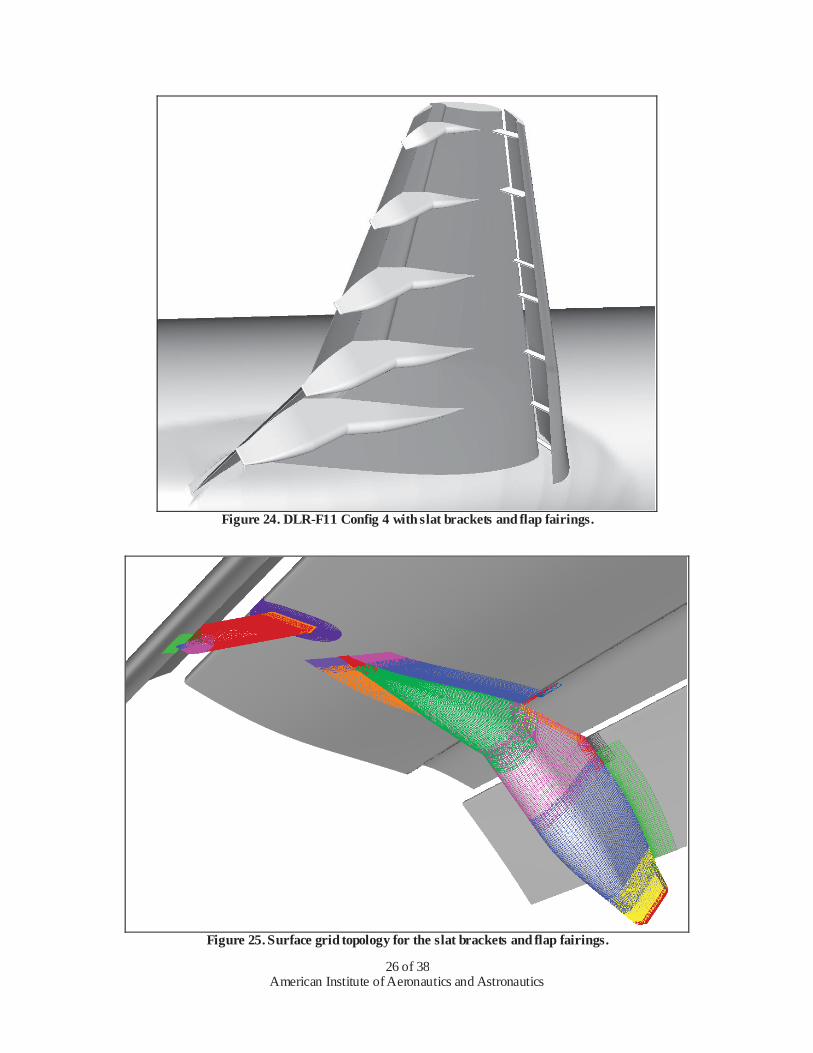
previous section with the addition of slat brackets and flap fairings. This geometry, referred to as Config 4, is more representative of the as-tested configuration. Figure 24 is an image of the Config 4 geometry showing the seven slat brackets and five flap fairings that were added to the medium mesh from the overset grid family. Slat bracket grids were generated using the Chimera Grid Tools (CGT) package while the flap support fairing surface grids were constructed using the ANSYS ICEM CFD meshing software. Volume grids for the flap supports were built using CGT. The addition of the brackets and fairings increased the total number of grid points from 69.0 million (see Table 2) to 97.2 million. Surface and volume grid images representative of all the brackets and fairings are provided in Figures 25 and 26, respectively. Using a standard equation for minimum wall spacing based on flat plate boundary layer theory, the y+ spacing for the medium grid has a value of 0.818 which is based on the higher Reynolds number of 15.1 million. The minimum cell size at the wall is 4.5 x10-4 mm. The exact same grid was used for the lower Reynolds number of 1.35 million which means the y+ value is roughly an order-of-magnitude smaller. The Boeing author has experience using grids with a very small y+ value, meaning there are more grid points packed in the boundary layer, for a Reynolds number study such as this one. For the purposes of this workshop, analyzing a high Reynolds number grid at low Reynolds number conditions will not have a significant effect on the DLR-F11 results.

Test Case 2 is intended to evaluate how well CFD predicts the effect of Reynolds number for a given high-lift configuration. By comparing the medium grid results between Test Case 1 and 2, the effect of brackets and fairings are computed as well. The discussion of results for this study is limited to force and moment comparisons as well as


9 of 38

surface streamline flow visualization intended to help identify flow features driving stall progression. More details of the flow field such as surface pressures and velocity profiles will be discussed in the next section.

The effect of brackets is illustrated in the lift curve comparison of Figure 27. Lift is reduced across the full range of alphas analyzed when the slat brackets and flap fairings are included which is a trend consistent with the Trap Wing results from HiLiftPW-1.7 Along with the bracket-off/on configuration effect, the code was run with and without QCR to quantify its effect on the Config 4 lift curve. With QCR, lift is increased slightly through the linear portion of the lift curve (7° ≤ ≤ 16°) for both configurations. The bracket-on, QCR-on dataset is the only one in Figure 27 that shows a clear lift break between 21° and 22.4° degrees. This finding, together with effects seen in the grid convergence study, suggests QCR significantly alters the DLR-F11 results in a favorable manner. The predicted stall is considered “favorable” because it is more in-line with experiment as indicated by the comparison in Figure 27. The QCR-on data presented in this figure clearly show that the addition of the slat brackets force stall to occur.

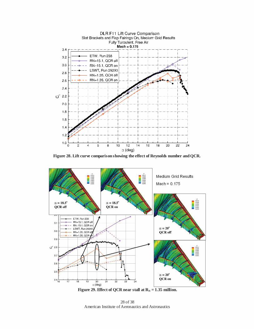
Variation in lift due to Reynolds number (RN) is given in Figure 28 where both the high (15.1 million) and low (1.35 million) RN results are compared against corresponding wind tunnel data. This comparison is for Config 4 where the brackets were analyzed. The OVERFLOW results are in agreement with test data in terms of the general trend where lower lift levels correspond to lower Reynolds number across the full range of angles -of-attack. The computed lift increment due to RN is significantly greater than the test data at a given alpha which is likely due to the fact that the CFD simulation does not account for any laminar boundary layer effects. This is an important discrepancy in the CFD-to-experiment comparisons particularly for lower RN where transitional effects are present in the wind tunnel data.

Figure 28 includes a full set of QCR-on/off data for both Reynolds numbers. The effect of QCR is noticeable in the lift curves where stall is predicted to occur at lower angles-of-attack when the nonlinear stress model is activated. This result pulls the OVERFLOW lift curves into better agreement with experiment, particularly for the higher RN data. A qualitative evaluation of the flow field near the computed stall boundary is made in Figure 29 to identify the region where QCR forces stall to occur at a lower angle. The lift curve in Figure 29 contains the same data plotted in Figure 28 with a tighter scale around CLmax. The surface streamline image comparisons at 18.5° and 20° indicate QCR has little effect on the surface flow features prior to stall. A much larger difference is seen at 20° where the QCR-on solution is characterized by a large wedge-shaped region of separated flow on the wing’s upper surface behind slat bracket 6 (roughly 80% semi-span). This predicted lift break-down is studied in more detail in the next section with the pressure tube bundles included.

D. Test Case 3 – Full Configuration Study The primary goal of the full configuration study is to quantify the effect of slat pressure tube bundles (PTB) on

the high-lift flow field. The medium grid built for the grid convergence study of Test Case 1 and modified to include slat and flap support hardware for the Reynolds number study of Test Case 2 was modified again to include PTB geometry. With the addition of this geometry came the need for local grid refinement which will be briefly discussed in this section. Based on the results from Test Case 1 and 2, all OVERFLOW runs for the full configuration study were made with QCR turned on.

The bundles were present on the DLR-F11 wind tunnel model whenever static surface pressure data was recorded on the slat. As shown in Figure 30, the PTB consisted of multiple flexible tubing bundled together and tied -off to the adjacent slat bracket. A simple representation of the bundles is presented in Figure 30 as the red tube in the image on the right side of the figure. This simplified geometry was provided to workshop participants for grid generation of the full configuration referred to as “Config 5.” Figure 31 provides a full-span view of the slat brackets, PTB and wing leading-edge with the slat not shown for clarity. There are a total of seven slat brackets (blue objects in Figure 31) and nine bundles (red objects). The two brackets nearest the wing tip have bundles on either side as shown in the inset image for bracket 6. For discussion purposes, the brackets are labeled 1-7 with the most inboard location being 1.

While the local surface grid resolution provided acceptable overlap characteristics (i.e., comparable cell size) between the PTB and slat/wing intersecting surfaces, a grid refinement exercise was conducted to ensure sufficient off-body grid resolution. This refinement study consisted of adding a patch grid to the upper surface of the main wing element behind each of the seven slat brackets. These surface abutting grids started in the chord direction just below the wing’s leading-edge highlight to pick-up the bracket and PTB wake flow, and they ended at the wing trailing-edge. A planform view of the L=1 (i.e., surface) grid plane for each patch grid is shown in Figure 32. Each patch grid was constructed using surface streamlines from a RN = 1.35 million solution at 7° angle-of-attack. The area each patch grid covers in the span direction was based on surface flow features prior to stall. After the initial set of patch-grid-on results were analyzed, the patch behind bracket 6 (purple grid in Figure 32) was made wider to


10 of 38

cover more of the wing span in this critical outboard region. The revised “dense” patch grid 6 is shown in Figure 33. The effect of the patch grids will be discussed throughout this Test Case 3 results section.

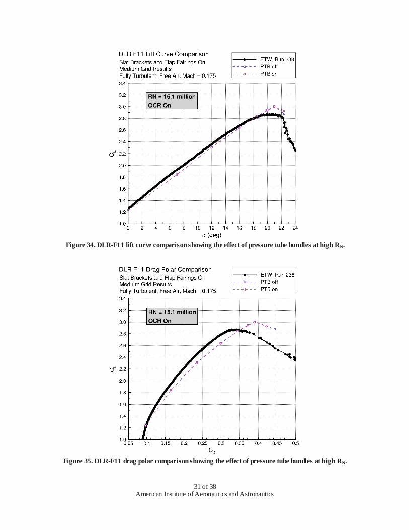
The lift curve comparison in Figure 34 includes high Reynolds number results with the pressure tube bundles off and on. There is very little effect predicted across the full range of angles analyzed. The same can be said for the drag and pitching moment data plotted in Figures 35 and 36, respectively. The PTB-on results are essentially the same as the PTB-off data, so OVERFLOW does not predict a significant PTB effect on forces and moments for the DLR-F11 wind tunnel model at a Reynolds number of 15.1 million.

Figure 37 is a lift curve comparison for the full configuration at RN = 1.35 million. Similar to the high RN results, the PTB do not have an effect at angles-of-attack below 16°. Above this angle, significant differences in computed lift are predicted when the PTB are added. CL at 18.5° falls well below the PTB-off data as well as below the wind tunnel lift curve. The large difference in lift level near stall was only seen when the PTB were analyzed without the patch grids shown in Figures 32 and 33. The solutions with the patch grids included have higher lift levels at 18.5° and above as shown in Figure 37. Similar trends are seen in the drag and pitching moment comparisons of Figures 38 and 39. That is, when the bundles are modeled with the wing patch grids included, the results are similar to the PTB-off data. Without the patch grids, the PTB-on force and moment data stand apart at higher angles -of-attack.

A series of surface flow visualization images are compared in Figures 40 and 41 to better understand the trends in lift at 18.5° and 21°. Both figures include an oil flow image from the low Reynolds number wind tunnel test with the corresponding OVERFLOW solution images stacked across the bottom of the figure. The wind tunnel image at

= 18.5° in Figure 40 has two wedge-shaped regions of separation on the main wing element at the trailing-edge. The larger separation region is located roughly at the mid-span station behind slat bracket 5 and the second, slightly smaller separation region is located behind bracket 6. Neither of these regions extend forward to the main element’s leading-edge, so the separation is not across the entire airfoil chord suggesting a pre-stall condition was captured in the photo. The experimental data in Figure 37 supports this conclusion as the lift curve at 18.5° has not “rounded -over.” The four CFD images across the bottom of Figure 40 are for the same flow condition as the wind tunnel image. These CFD images, labeled A through D, are briefly described below.

Image A: Case 2a, brackets-on, PTB-off, wing patch grids-off Image B: Case 3a, brackets-on, PTB-on, wing patch grids-off Image C: Case 3a, brackets-on, PTB-on, wing patch grids-on Image D: Case 3a, brackets-on, PTB-on, wing patch grids-on with dense patch grid behind bracket 6

To anchor the surface flow comparison, a dashed horizontal line is drawn across the four solution images marking the approximate location of bracket 5. The first thing to note in this comparison is the lack of any boundary layer separation behind bracket 5 in the OVERFLOW solutions. Adding the pressure tube bundles and refining the grid did not trigger mid-span wing separation seen in the test data at this condition. There are differences behind bracket 6 however. Figure 40 clearly shows how the addition of PTB causes wing separation to develop behind bracket 6 which is roughly at a semi-span station of 80%. This large region of outboard wing separation is the reason for the reduction in loading seen in the lift curve comparison of Figure 37. Grid refinement, by way of adding wing patch grids, reduces the extent of the separation to a region of comparable size with the wind tunnel flow visualization image. Another interesting observation to be made in the CFD images of Figure 40 is the effect patch grids (i.e., grid refinement) have on skin friction contours. By comparing image B and C, it is easy to see how the red streaks behind the inboard slat brackets are better defined suggesting a more resolved vortical flow field. The surface flow visualization images in Figure 41 tell a slightly different story for an angle-of-attack of 21°. At this angle, the wind tunnel image captured a large region of mid-span wing separation behind bracket 5 compared to the image in Figure 40. This separation appears to be of the full-chord type suggesting stall has occurred which is supported by the experimental lift curve. The OVERFLOW solutions on the bottom half of Figure 41 show how the addition of PTB causes the code to predict wing separation behind bracket 5 as seen in the test data. However, when the grid is refined in the wake region of each of the slat brackets and PTB, the mid-span separation is no longer predicted. In fact, the C and D images are similar to the PTB-off solution image A. This trend is troubling to say the least and leaves the authors speculating that something is being missed in the CFD simulation such as transitional flow modeling and/or unsteady effects. The latter of which will be discussed in the following paragraphs. Before discussing the low Reynolds number time accurate analysis, off-body flow visualization images are compared in Figure 42 to further illustrate the effect of PTB and grid refinement at 18.5° and 21°. The stack of CFD images in this figure is an isometric view of the wing upper surface showing constant vorticity surfaces behind slat brackets 4, 5 and 6. The effect of adding wing patch grids behind each bracket/PTB is unmistakable. The vortical


11 of 38

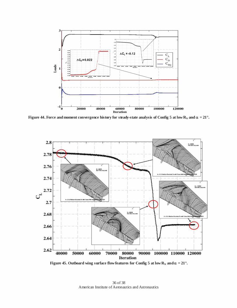
wake flow is better resolved in the lower two images where the patch grids were analyzed (note that these solutions correspond to Image D in Figures 40 and 41. As noted above, residual convergence of the flow solver and turbulence model is poor at best, but steady-state forces do converge (with small oscillations about a well defined mean) for most cases. The convergence of lift coefficient for Config 5 at = 7.0°, 16.0° and 18.5° are shown in Figure 43. The mean lift converges for the three angles at about 20,000 iterations and has a consistent mean over the next 50,000 iterations. Figure 44 shows a different story for = 21°, there is a slow drop in CL and slight increase in CD from about 20,000 iterations until about 70,000 iterations and then a rapid change over the next 3,000 iterations where CL drops by 4% (-0.12) and CD increases by 6% (220 counts) and then reaches respective constant means. Figure 45 shows particle traces on the wing surface at different points, (N=40,000, 80,000, 96,000 and 120,000), along the convergence of the = 21° case, showing that the main difference across solutions is the size of the separation at the slat bracket 6 span location. Normal force semi-span loading for the 4 points in the iteration is shown in Figure 46, which also shows that only the tip loading changes across the cases. It is known that inaccuracy in mean-flow quantities can result from computing unsteady flows with the stead-state (time-inaccurate) integration scheme. The high-frequency oscillation seen in the integrated loads of many simulations presented here suggests unsteady flow. The pre-stall, non-time-accurate Config 5 case at = 16° was restarted time accurately (at N = 30,000) with 10 inner dual iterations (giving at least 1 order of magnitude drop in inner iteration residual) at a physical time step of 0.35 which translates into approximately 1000 time steps to travel 1 mean aerodynamic chord length. Figure 47 shows that the resulting change in CL (0.8 %) and CD (0.7%) is insignificant and an analysis of the flow field shows little variation except in the flap trailing edge region. The Config 5 = 21° case was restarted at 4 test solution points shown in Figure 45 and the resulting convergence of CL and CD are shown in Figure 48. In all cases, the loads exhibit an unsteady damp oscillation to the converged consistent values. Even though the starting values are significantly different, the resulting CL = 0.011 (0.4%) and

CD = 24 counts (0.6%) fall well within computing errors. Figure 49 gives more detail as to the differences (mainly the slat bracket 6 separation bubble size) along the convergence path of the case starting at N = 80,000 non-time-accurate result to the time accurate result. These results emphasize the importance of time accurate analysis, especially in the stall regions. Finally, a few observations and speculations as to the issue of accurately modeling stall. The following comments are based on the general workshop results, Rumsey, et al.4, the AIAA SciTech 2014 presentations,4,19,20,2122,23,24 and our current results. A number of contributors assessed the various effects of turbulence models,4,19,20,22,23 transition,4,21 time accuracy,4,22 and a wide variety of solver approaches, grid refinements, and accuracy.4 In almost all cases, the stall boundary was closely approximated, even though the stall mechanism (location of slat bracket/pressure tube bundle induced separation) did not show good correlation with experimental evidence. For example, the Config 5 = 21° experimental results show a large wedge shape separation at the 5th slat bracket location (see Figure 41), while computed results show separation at the 6th slat bracket location. Speculation and analysis of computed results as to the effects of transition modeling, turbulence model issues, and grid resolution of the slat bracket/ pressure tube bundle are all inconclusive. Unfortunately, experimental data for transition is only available for the low-Reynolds number cases, which is not representative of flight conditions. The grid resolution computational studies did not produce the right effect, even though the disturbances due to the vortical flow of the slat brackets and pressure tube bundles seem to be well resolved. Turbulence model variation did have an effect on the size and extent of the separated regions, but no clear trend toward correlation with the experimental stall mechanisms has been established. There seems to be a missing elemental key to getting the correct stall for this configuration, although one could speculate that better transition/turbulence modeling combined with good resolution and accuracy could produce better results. The stall mechanism for this configuration is controlled by the slat bracket effects and is not the same as the slat leading edge stall found on the Trap Wing model in HiLiftPW-1,13 and in our opinion a more difficult process to model. Another possibility for the discrepancy may be in the turbulence modeling of the effect of the vortical flow generated in the slat bracket regions, suggesting, just as in the case of QCR,18 that another form of rotation correction is needed. Consideration must also be given to the fact that the true geometry of the PTB is not being modeled.

VI. Conclusion The DLR-F11 high-lift wind tunnel model was analyzed using OVERFLOW in response to the 2nd AIAA CFD

High Lift Prediction Workshop. The analysis addressed all of the workshop’s required test cases and all but one of the optional test cases – boundary layer transition modeling was not attempted. The test cases were designed to quantify the effect of grid refinement, model support brackets, pressure tube bundles and Reynolds number on the


12 of 38

high-lift flow field. Unique aspects of this OVERFLOW analysis include the application of a quadratic constitutive relation (QCR) to the DLR-F11 simulation, localized grid refinement behind the slat brackets and a thorough time accurate study.

Grid refinement was investigated by first constructing a family of structured overset grids appropriate for use in grid convergence studies. This was accomplished by creating a medium-sized mesh following established guidelines for high-lift design studies as well as lessons learned from the first High Lift Prediction Workshop. For the DLR-F11 model, the medium overset mesh consisted of 69.0 million points. A less dense “coarse” mesh and two denser “fine” and “extra-fine” meshes were built from the medium mesh by systematically removing or adding points. The four grids of the overset family ranged in size from 29.4 million points up to 544.5 million points. All of the grids were analyzed at angles-of-attack of 7°, 12° and 16°, and the coarse/medium/fine grids were analyzed at the optional angles of 18.5°, 20°, 21° and 22.4°. The initial set of solutions exhibited unexpected lift convergence behavior driven by slowly developing side-of-body vortical flow features. A quadratic constitutive relation recently added to OVERFLOW to improve solution accuracy for corner flows was activated and the results improved. With the constitutive relation turned-on, variation in total lift coefficient was close to linear as the grid was refined for the lower angles-of-attack. Solutions above 16° were not dominated by the side-of-body flow field, so QCR had the most influence over the middle and outer span regions for the medium mesh solutions.

A Reynolds number study was conducted using the medium mesh from the grid refinement study. A set of seven slat brackets and five flap fairings were added to the grid to make the simulation more closely represent the as-tested configuration. The effect of QCR on stall characteristics was also investigated at both high RN (15.1 million) and low RN (1.35 million). The measured lift reduction through the linear portion of the lift curve due to the lower Reynolds number was over-predicted by OVERFLOW which may be partially due to the lack of laminar boundary layer regions in the CFD. The lower RN is expected to have more transitional flow features than at higher RN, so a fully turbulent simulation will have more error associated with thicker boundary layers and reduced lift levels. The effect of QCR was most pronounced at angles -of-attack above 18.5° where it forced outboard wing separation to occur behind slat bracket 6 which is located at a semi-span station of about 80%.

The geometric fidelity of the CFD model was elevated by including simulated pressure tube bundles (PTB) next to each slat bracket. The focus of this full configuration study was on the bundle’s impact to the flow field and predicted stall characteristics at both low and high Reynolds number. The low RN solutions at high angles were much more sensitive to the presence of the PTB compared to high RN results. Off-body grid refinement was found to be necessary for improved resolution of the bracket/bundle wakes. Depending on whether or not the bundles were modeled and local grid refinement was included, the low RN wing separation at = 21° moved between slat bracket 5 and 6 with varying degrees of span extent. This inconsistency with configuration and grid resolution in the low RN results led to the speculation that modeling transitional effects and/or time accuracy are important considerations when attempting to simulate stall characteristics of the DLR-F11.

An in-depth time accurate analysis was performed for the full configuration (Config 5) at the low RN condition to explore details of high-alpha force convergence, stall boundary prediction and associated flow field characteristics. Switching from a non-time-accurate to a time accurate simulation had little impact on the results for angles-of-attack below 21°. However, at this angle, running an unsteady simulation had a s ignificant effect on lift convergence. The development of outboard wing separation behind slat bracket 6 was accelerated with a time accurate approach compared to running in steady-state mode. Because the steady-state solution required an inordinate number of iterations to converge to the same state as the time-accurate run, it is considered beneficial to follow a time accurate approach for the higher angles-of-attack where outboard wing stall dominates the flow field.

Acknowledgments The authors thank the National Aeronautics and Space Administration and The Boeing Company for their

support in the 2nd AIAA CFD High Lift Prediction Workshop. Special thanks to William Chan at NASA Ames Research Center for overset grid guidance and to John Vassberg, Neal Harrison and Yoram Yadlin at Boeing for their assistance in generating grids.

References 1Levy, D., Laflin, K., T inoco, E., Vassberg, J., Mani, M., Rider, B., Rumsey, C., Wahls, R., Morrison, J., Brodersen, O.,

Crippa, S., Mavriplis, D., Murayama, M., “Summary of Data from the Fifth Computational Fluid Dy namics Drag Prediction Workshop,” AIAA Paper 2013-0046, 51st AIAA Aerospace Sciences Meeting, Grapevine, Texas, January 2013.

2Heeg, J., Ch walowski, P., Florance, J., Wieseman, C., Schuster, D. , and Perry, B. III, “Overview of the Aeroelastic Prediction Workshop,” AIAA 2013-0783, 51st AIAA Aerospace Sciences Meeting, Grapevine, Texas, January 2013.


13 of 38

3Rumsey, C., Slotnick, J., Long, M., Stuever, R., Wayman, T ., “Summary of the First AIAA CFD High -Lift Prediction Workshop,” Journal of Aircraft, Vol. 48, No. 6, 2011, pp. 2068 -2079.

4Rumsey, C., Slotnick, J., “Overview and Summary of the Second AIAA High Lift Prediction Workshop ,” AIAA 2014-0747, 52nd AIAA Aerospace Sciences Meeting, National Harbor, Maryland, January 2014.

5Rudnik, R., Huber, K., Melber-Wilkending, S., “EUROLIFT Test Case Description for the 2nd High Lift Prediction Workshop,” AIAA 2012-2924, 30th Applied Aerodynamics Conference, New Orleans, Louisiana, June 2012.

6Sclafani, A., DeHaan, M., Vassberg, J., Rumsey, C., Pulliam, T ., “Drag Prediction for the NASA CRM Wing-Bo dy-Tail Using CFL3D and OVERFLOW on an Overset Mesh ,” AIAA 2010-4219, 28th Applied Aerodynamics Conference, Chicago, Illinois, June 2010.

7Sclafani, A., Slotnick, J., Vassberg, J., Pulliam, T ., Lee, H. “OVERFLOW Analysis of the NASA Trap Wing Model from the First High Lift Prediction Workshop ,” AIAA 2011-0866, 49th AIAA Aerospace Sciences Meeting, Orlando, Florida, Jan uary 2011. 8Fisher, M., Michal, T ., Cary, A., “MADCAP User’s Guide,” URL: http://www.grc.nasa.gov/WWW/winddocs/madcap/madcap.pdf, Version 2.15. 92nd AIAA CFD High Lift Prediction Workshop, URL: http://hiliftpw.larc.nasa.gov/, email: [email protected], June 2013. 10Nash, S. M., Rogers, S. E., “Manual for Scripts,” URL: http://rotorcraft.arc.nasa.gov/cfd/CFD4/CGT/scripts.html, January 2008. 11Chan, W. M., Rogers, S. E., Pandya, S. A., Kao, D. L., Buning, P. G., Meakin, R. L., Boger, D. A., Nash, S. M., “Chimera Grid Tools User’s Manual,” URL: http://people.nas.nasa.gov/~wchan/cgt/doc/man.html, Version 2.1, March 2010. 12Chan, W. M., Chiu, I. T ., Buning, P. G., “User’s Manual for the HYPGEN Hyperbolic Grid Generator and the HGUI Graphical User Interface,” NASA TM 108791, October 1993. 13Suhs, N. E., Rogers, S. E., Dietz, W. E., “PEGASUS 5: An Automated Pre-processor for Overset-Grid CFD,” AIAA Paper 2002-3186, 32nd AIAA Fluid Dynamics Conference, St. Louis, MI, June 2002. 14Nichols, R., Buning, P., “User’s Manual for OVERFLOW Version 2.2,” August 2010.

15Spalart, P. R., Allmaras, S. R., “A One-Equation Turbulence Model for Aerodynamic Flows,” AIAA Paper 92-0439, January 1992.

16Nichols, R. H., “Algorithm and Turbulence Model Requirements for Simulating Vortical Flo ws,” AIAA Paper 2008 -0337, 46th AIAA Aerospace Sciences Meeting, Reno, NV, January 2008.

17Sclafani, A., Vassberg, J., Winkler, C., Dorgan, A. Mani, M., Olsen, M., Coder, J., “DPW -5 Analysis of the CRM in a Wing-Body Configuration Using Structured and Unstructured Meshes,” AIAA 2013-0048, 51st AIAA Aerospace Sciences Meeting, Grapevine, Texas, January 2013.

18Spalart, P. R., “Strategies for turbulence modelin g and simulations,” International Journal of Heat an d Fluid Flo w, Vol. 21 (2000) pp. 252-263.

19Mavriplis, D., Long, M., Lake, T ., Langlois, M., “ NSU3D Results for the Second AIAA High Lift Prediction Workshop”, AIAA 2014-0748, 52nd AIAA Aerospace Sciences Meeting, National Harbor, Maryland, January 2014.

20Eliasson, P., Peng, S., “ Results for the 2nd AIAA High Lift Prediction Workshop using Edge”, AIAA 2014-0750, 52nd AIAA Aerospace Sciences Meeting, National Harbor, Maryland, January 2014.

21 Konig, B., Fares, E., Nolting, S., “ lattice-Boltzmann Flow Sim ulations for the HiLiftPW-2”, AIAA 2014-0911, 52nd AIAA Aerospace Sciences Meeting, National Harbor, Maryland, January 2014.

22Deloze, T ., Laurendeau, E., “NSMB Contribution to the Second AIAA High Lift Prediction Workshop”, AIAA 2014 -0913, 52nd AIAA Aerospace Sciences Meeting, National Harbor, Maryland, January 2014.

23Hanke, J., Shankara, P., Snyder, D., “Numerical Simulation of DLR-F11 High Lift Configuration from HiLiftPW-2 using STAR-CCM+”, AIAA 2014-0914, 52nd AIAA Aerospace Sciences Meeting, National Harbor, Maryland, January 2014.

24Rudnik, R., Melber-Wilkending, S., “DLR Contribution to the 2nd AIAA High Lift Prediction Workshop”, AIAA 2014 -0915, 52nd AIAA Aerospace Sciences Meeting, National Harbor, Maryland, January 2014.


14 of 38

Figure 1. DLR-F11 high-lift wind tunnel model in the Airbus Low Speed Tunnel in Bremen (B-LSWT).

Figure 2. DLR-F11 flap seal at the side-of-body.


15 of 38

Figure 3. F11 overset surface grid layout: Config 2, coarse mesh.

Figure 4. F11 Config 2 surface grids for the coarse mesh with spanwise clustering highlighted.


16 of 38

Figure 5. Simplified illustration of the grid family relationship.

Figure 6. Surface grid comparison for the inboard slat and wing.


17 of 38

Figure 7. Surface grid comparison for the inboard wing and flap.

Figure 8. Surface grid comparison for the outboard slat, wing and flap.


18 of 38

Figure 9. Off-body coarse grid near the wing trailing-edge break.

Figure 10. DLR-F11 convergence history for lift: Brackets-off, Mach = 0.175, RN = 15.1 million.


19 of 38

Figure 11. DLR-F11 residual convergence history: Brackets-off, Mach = 0.175, RN = 15.1 million.

Figure 12. Region of flow field that develops the slowest at = 7°.


20 of 38

Figure 13. Surface streamlines and off-body flow features at side-of-body for = 7°.

Figure 14. Effect of QCR on lift convergence and side-of-body separation.


21 of 38

Figure 15. Effect of grid resolution and QCR on lift for the DLR-F11 Config 2 geometry.

Figure 16. Bracket-off lift curves at RN=15.1 million showing the effect of grid resolution and QCR.


22 of 38

Figure 17. Effect of grid resolution and QCR on drag for the DLR-F11 Config 2 geometry.

Figure 18. Bracket-off drag polars at RN=15.1 million showing the effect of grid resolution and QCR.


23 of 38

Figure 19. Effect of grid resolution and QCR on pitching moment for the DLR-F11 Config 2 geometry.

Figure 20. Bracket-off pitching moment at RN=15.1 million showing the effect of grid resolution and QCR.


24 of 38

Figure 21. Surface streamline comparison for the DLR-F11 Config 2 geometry.


25 of 38

Figure 22. Off-body flow visualization highlighting the areas of difference caused by using QCR.

Figure 23. Sectional lift comparison for the DLR-F11 Config 2 geometry.


26 of 38

Figure 24. DLR-F11 Config 4 with slat brackets and flap fairings.

Figure 25. Surface grid topology for the slat brackets and flap fairings.


27 of 38

Figure 26. Off-body grid image of flap fairing at Y=1348 mm.

Figure 27. Lift curve comparison showing the effect of brackets and QCR.


28 of 38

Figure 28. Lift curve comparison showing the effect of Reynolds number and QCR.

Figure 29. Effect of QCR near stall at RN = 1.35 million.


29 of 38

Figure 30. Bracket and pressure tube bundle comparison between wind tunnel model (left) and CFD (right).

Figure 31. Brackets and pressure tube bundles used for CFD simulations (slat not shown for clarity).


30 of 38

Figure 32. Wing planform view showing surface grid planes of PTB patch grids.

Figure 33. Wing planform view showing surface grid planes of PTB patch grids with increased size/density

behind bracket 6 (purple grid).


31 of 38

Figure 34. DLR-F11 lift curve comparison showing the effect of pressure tube bundles at high RN.

Figure 35. DLR-F11 drag polar comparison showing the effect of pressure tube bundles at high RN.


32 of 38

Figure 36. DLR-F11 pitching moment comparison showing the effect of pressure tube bundles at high RN.

Figure 37. DLR-F11 lift curve comparison showing the effect of pressure tube bundles at low RN.


33 of 38

Figure 38. DLR-F11 drag polar comparison showing the effect of pressure tube bundles at low RN.

Figure 39. DLR-F11 pitching moment comparison showing the effect of pressure tube bundles at low RN.


34 of 38

Figure 40. Surface flow visualization showing effect of PBT and patch grids at low RN and = 18.5°.

Figure 41. Surface flow visualization showing effect of PTB and patch grids at low RN and = 21°.


35 of 38

Figure 42. Off-body flow visualization showing effect of PTB and patch grids at low RN.

Figure 43. Lift convergence for Config 5 at low RN, = 7°, 16°, 18.5°.


36 of 38

Figure 44. Force and moment convergence history for steady-state analysis of Config 5 at low RN and = 21°.

Figure 45. Outboard wing surface flow features for Config 5 at low RN and = 21°.


37 of 38

Figure 46. Semi-span loading at selected points in convergence of Config 5 at low RN and = 21°.

Figure 47. Lift and drag convergence from non-time-accurate to time accurate, Config 5 at low RN, = 16°.


38 of 38

Figure 48. CL and CD convergence history for time accurate analysis of Config 5 at low RN and = 21°.

Figure 49. Time accurate convergence starting from non-time-accurate at 80,000 iterations.

High-Lift OVERFLOW Analysis of the DLR-F11 Wind … · High-Lift OVERFLOW Analysis of the DLR-F11...

Documents

Transcript of High-Lift OVERFLOW Analysis of the DLR-F11 Wind … · High-Lift OVERFLOW Analysis of the DLR-F11...