High-Level Synthesis of a MPEG-4 Decoder Using SystemC

Kgs. Lyngby 2003 IMM-THESIS-2003-64

Gomu Miyashita

High-Level Synthesis of a MPEG-4 Decoder Using SystemC

Gomu Miyashita

High-Level Synthesis of a MPEG-4 Decoder

using SystemC

Kgs. Lyngby 2003

Technical University of Denmark Informatics and Mathematical Modelling Building 321, DK-2800 Lyngby, Denmark Phone +45 45253351, Fax +45 45882673 [email protected] www.imm.dtu.dk IMM-THESIS: ISSN 1601-233X

1

Preface

This Master’s Thesis was written at the Department of Informatics and Mathematical

Modelling at the Technical University of Denmark during April 2003 - October 2003

with supervisor Hans Holten Lund, IMM and assistant supervisor Søren Forchhammer,

COM.

Author is Gomu Miyashita (s938493).

Kgs. Lyngby, October 31, 2003

_____________________________________

Gomu Miyashita

3

Abstract

This report presents a simulation model of a hardware MPEG-4 Simple@L0 compliant

video decoder for behavioral synthesis. The report deals with the subset of the MPEG-4

standard that deals with low-bitrate coding of rectangular natural video. An open source

project, known as XviD, serves as the basis for this project. XviD is a software

implementation of a MPEG-4 compliant video CODEC (Coder and Decoder) written in C.

Modeling was done using the SystemC hardware description language, and according to

the rules for behavioral modeling, described in the Synopsys documentation. Synopsys

synthesis tools enable behavioral synthesis and implementation. These tools were used to

synthesize part of the model. A full synthesis of the model has not been performed. A

major part of this project was to rewrite the XviD software CODEC to a synthesizable

behavioral model in SystemC. This process involved separating the decoder from the

encoder parts, replacing non-synthesizable programming structures with synthesizable

alternatives, and designing an architecture that promote parallel processing. A lot of

effort was put into reducing on chip memory requirements. The results of these findings

will be presented with a discussion on the use of SystemC as a modeling language for

behavioral synthesis. Test results will be presented with estimation of internal band width

requirements. Finally some ideas are proposed on future work of the decoder.

Keywords: Behavioral modeling, SystemC, MPEG-4 decoding, behavioral synthesis,

digital video.

5

Resume

Denne rapport præsenterer en simulerings model af en hardware MPEG-4 Simple@L0

kompatibel video dekoder. Rapporten omhandler den del af MPEG-4 standarden som har

med low-bitrate kodning af rektangulær natulig video. Et open-source project, kaldet

XviD, er udgangspunktet for projektet. XviD er en software implementering af en

MPEG-4 video CODEC (Coder/Decoder) skrevet i C. Modellen blev implementeret i

SystemC og i overenstemmelse med Synopsys dokumentationen. Synopsys syntese

værktøjer muliggør høj niveau syntese og implementering. Disse værktøjer blev brugt til

at syntetisere dele af modellen. Syntese af hele modellen er ikke foretaget. En stor del af

projektet var omskrivning af XviD CODEC til en syntetiserbar højniveau model i

SystemC. Denne process inkluderede isolering af dekoder-delen fra enkoder-delen,

omskrivning af ikke-syntetiserbar kode til syntetiserbare alternativer, samt design af en

arkitektur som muliggør parallelisering af beregninger. En del tid blev envidere brugt på

at minimere brugen af den intern hukommelse. Resultatet af omskrivningen samt en

diskussion af SystemC som modellerings sprog til højniveau syntese er inkluderet i

rapporten. Test resultater er præsenteret med en estimering af interne båndbredde krav.

Nogle forslag til videre arbejde med modellen er givet sidst i rapporten.

Nøgleord: Højniveau modellering, SystemC, MPEG-4 decodning, højniveau syntese,

digital video.

7

Acronyms

2D 2-Dimensional

3D 3-Dimensional

3G Third Generation

3GPP Third Generation Partnership Project

ASF Advanced Streaming Format

CBR Constant Bit Rate

CODEC Coder and Decoder

DCT Discrete Cosine Transform

DVD Digital Versatile Disc

EMS Enhanced Message Service

FIFO First In First Out

FPGA Field Programmable Gate Array

GMC Global Motion Compensation

GOV Group of Video Object Planes

GSM Global Systems for Mobil Communication

HDL Hardware Description Language

IDCT Inverse Discrete Cosine Transform

ISDN Integrates Services Digital Network

LAN Local Area Network

LBR Low Bit rate Coding

MB Macroblock

MMS Multimedia Message Service

MP3 MPEG Audio Layer 3

MV Motion Vector

QCIF Quarter Common Intermediate Format

RTL Register Transfer Level

SMS Short Message Service

VBR Variable Bit Rate

VCD Video Compact Disc

8

VLC Variable Length Code

VOP Video Object Plane

WMA Windows Media Audio

WMV Windows Media Video V3

9

Table of Contents

Preface................................................................................................................................. 1 Abstract ............................................................................................................................... 3 Resume................................................................................................................................ 5 Acronyms............................................................................................................................ 7 Table of Contents................................................................................................................ 9 1 Introduction............................................................................................................... 13 2 Basics of MPEG-4 Digital Video ............................................................................. 17

2.1 Colorspace......................................................................................................... 17 2.2 MPEG-4 Terminology ...................................................................................... 18 2.3 Basic MPEG-4 Encoding.................................................................................. 21

2.3.1 Motion estimation ............................................................................................ 22 2.3.2 Texture coding ................................................................................................. 22

2.4 MPEG-4 ............................................................................................................ 23 2.4.1 Profile and Levels ............................................................................................ 23 2.4.2 Natural Video................................................................................................... 24

2.5 Summary........................................................................................................... 25 3 MPEG-4 Video Decoding Process............................................................................ 27

3.1 Texture Decoding.............................................................................................. 28 3.1.1 DC and AC Prediction Direction ..................................................................... 30 3.1.2 Inverse Quantization ........................................................................................ 32

3.1.2.1 First Inverse Quantization Method ........................................................... 32 3.1.2.2 Second Inverse Quantization Method....................................................... 33 3.1.2.3 Saturation .................................................................................................. 34

3.1.3 Inverse DCT..................................................................................................... 34 3.2 Motion Decoding .............................................................................................. 35

3.2.1 Padding ............................................................................................................ 35 3.2.2 Half sample interpolation................................................................................. 35 3.2.3 Unrestricted motion compensation .................................................................. 36 3.2.4 Vector decoding............................................................................................... 38 3.2.5 Vector prediction ............................................................................................. 39

3.3 Error resilience.................................................................................................. 40 3.3.1 Slice resynchronization.................................................................................... 40 3.3.2 Data partitioning .............................................................................................. 41 3.3.3 Reversible VLC ............................................................................................... 41

3.4 Simple@L0 ....................................................................................................... 41 3.5 Summary........................................................................................................... 42

4 Implementation ......................................................................................................... 45 4.1 Behavioral Modeling ........................................................................................ 45 4.2 Converting to Synthesizable Subset of SystemC.............................................. 46

4.2.1 Pipelining Loops .............................................................................................. 48 4.2.2 Signals.............................................................................................................. 48

4.3 Structure............................................................................................................ 49 4.3.1 Texture decoding ............................................................................................. 50

10

4.3.2 Motion decoding .............................................................................................. 50 4.4 Communication................................................................................................. 51 4.5 Input/Output FIFO buffers................................................................................ 53 4.6 Modules............................................................................................................. 54

4.6.1 getBits .............................................................................................................. 55 4.6.2 Demux.............................................................................................................. 55

4.6.2.1 Header ....................................................................................................... 56 4.6.2.2 Motion....................................................................................................... 58 4.6.2.3 Texture ...................................................................................................... 59

4.6.3 Scan Prediction ................................................................................................ 60 4.6.3.1 Decoding VLC.......................................................................................... 62 4.6.3.2 AC/DC Prediction..................................................................................... 63

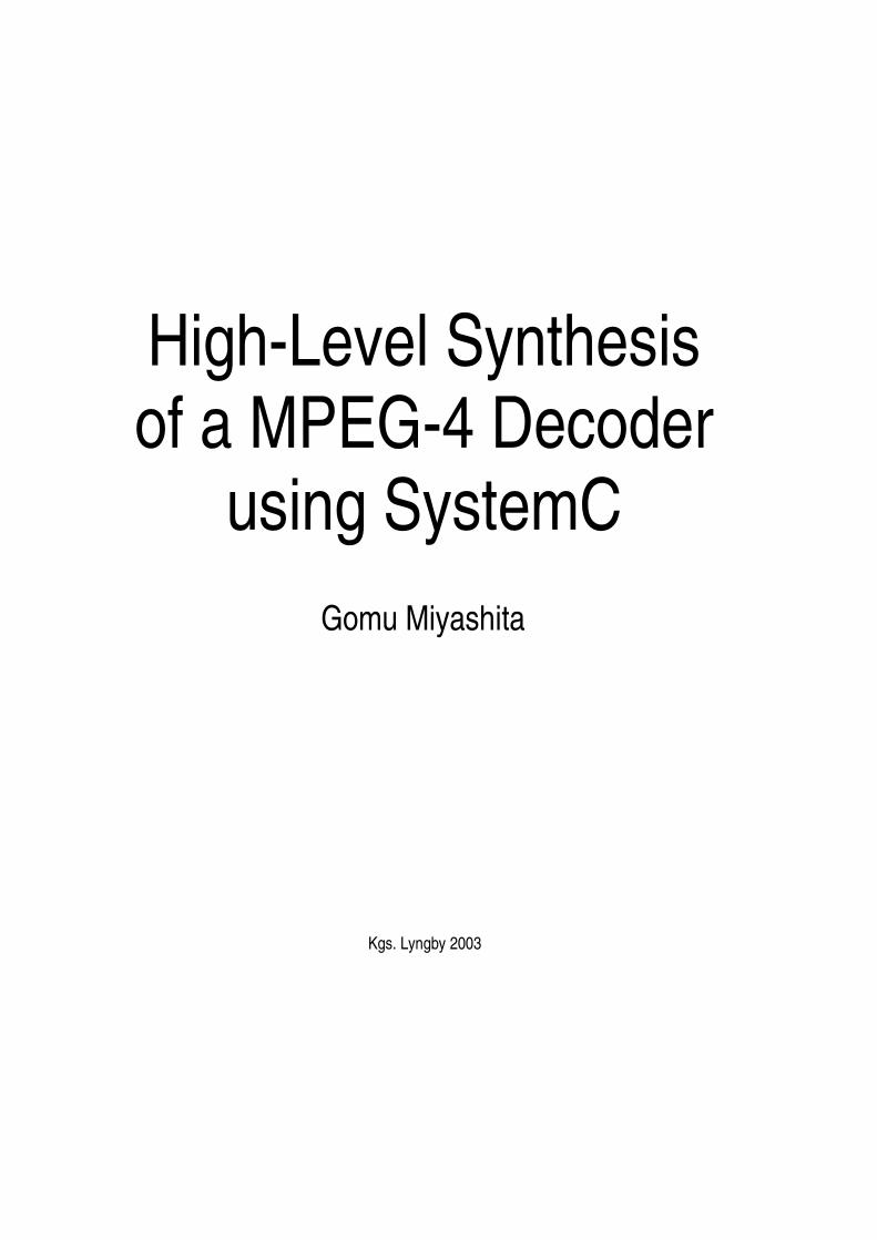
4.6.4 Tbuffer ............................................................................................................. 64 4.6.5 Quant................................................................................................................ 64 4.6.6 Idct ................................................................................................................... 66 4.6.7 MV Prediction.................................................................................................. 67 4.6.8 Mbuffer ............................................................................................................ 68 4.6.9 Interpolate ........................................................................................................ 69 4.6.10 Reconstruct .................................................................................................... 72 4.6.11 Memory Controller ........................................................................................ 74 4.6.12 Display ........................................................................................................... 77

4.6.12.1 YUV to RGB........................................................................................... 78 4.6.13 Output Generator ........................................................................................... 79

5 Testing....................................................................................................................... 81 5.1 Bitstream storage .............................................................................................. 81 5.2 Bitstream creation ............................................................................................. 82 5.3 Test results ........................................................................................................ 82 5.4 Bandwidth analysis ........................................................................................... 83 5.5 Synthesis ........................................................................................................... 83

6 Conclusion ................................................................................................................ 85 References......................................................................................................................... 89 7 Appendix A............................................................................................................... 91

MPEG-4 Background.................................................................................................... 91 Objectives ................................................................................................................. 91

XviD.............................................................................................................................. 93 8 Appendix B ............................................................................................................... 95

8.1 Encoder settings ................................................................................................ 95 9 Appendix C ............................................................................................................... 97

VOP Header .................................................................................................................. 97 MB Header.................................................................................................................... 98

10 Appendix D......................................................................................................... 101 10.1 BMP file format .............................................................................................. 101

11 Appendix E ......................................................................................................... 103 11.1 AVI File format............................................................................................... 103

12 Appendix F.......................................................................................................... 105 12.1 File structure ................................................................................................... 105

11

12.2 Simulating the model ...................................................................................... 106

13

1 Introduction

Short Message Service (SMS) is a service that enables GSM subscribers to send short

messages, of up to 160 characters, to one another. With an estimated 15 billion SMS

messages send every month, this service has proved extremely popular. The popularity of

instant messaging prompted the industry to develop services beyond simple text

messages. Enhanced Message Service (EMS) is an extension of the existing SMS

messaging service and allows users to include pixel-animations and melodies in messages.

EMS builds on existing network infrastructures and can be viewed as an intermediate

stage towards full multimedia support. Multimedia Messaging Service (MMS) is the next

generation of instant messaging and will support color pictures, animations, audio and

video. Mobile network operators around the world are currently deploying 3rd generation

(3G) networks, capable of delivering multimedia content. MPEG-4 Simple Profile has

been selected by the Third generation Partnership Project1 (3GPP) as the standard for

wireless video in 3G mobile networks. The stability, interoperability and robustness

offered by MPEG-4 makes it ideal for mobile networks.

The MPEG-4 Simple Profile was created with mobile visual services in mind amongst

others. The Simple Profile at level 0 (Simple@L0) was specifically developed at the

request of the 3GPP2. The MPEG-4 Simple@L0 support rectangular natural video with

frame rate of 15 fps in QCIF3 resolution and bit rates up to 64 Kbits/s.

Low bit rate multimedia transmission and exchange of MPEG-4 video content in a

mobile network require mobile phones that are capable of handling highly compressed

visual data. Consumption of low bit rate video requires mobile phones that are equipped

with low-cost and low-power decoding capabilities.

1 Third Generation Partnership Project: A group of telecommunication standard bodies to produce specification for the 3rd generation mobile system. 2 Profiles and levels are describes in Section 2.4.1. 3 144x176 pixels for luminance and 72x88pixels for chrominance.

14

This report presents a simulation model of a MPEG-4 Simple@L0 compliant video

decoder in hardware for real-time decoding in mobile phones. The decoder has been

modeled using behavioral modeling techniques.

Behavioral synthesis introduces a higher level of design abstraction and is defined as the

transformation of a behavioral description to a Register Transfer Level (RTL) description.

Synopsys tools were used for behavioral synthesis. These tools enable synthesis of

designs, implemented at the behavioral level, and generate synthesizable code at the RTL

level. The synthesis tools schedule operations into clock cycles and perform hardware

allocation, based on user constraints. This allows designers to control design parameters

such as latency, throughput, resource allocation and I/O activity without significant

changes to the source code.

SystemC is a C++ class library and enables design and simulation of hardware

descriptions in a software environment. SystemC allows designers to design and verify at

all levels of abstractions in a common language. A manual conversion from an abstract

architecture model in C++ to a detailed HDL RTL model can thus be avoided. The

Synopsys Behavioral Compiler is a high-level synthesis tool capable of generating RTL

code from a behavioral description. These tools show great promise in reducing time

from concept to implementation by reducing design iterations and simulation times.

Hardware design in SystemC using behavioral design methodology offers several

advantages. A software implementation of the algorithm, written in C++, can be

gradually converted to a SystemC hardware model within the software environment. The

model can, at any time, be verified for correctness in the software environment which

often reduces simulation times. The higher level of abstraction introduced also promotes

reuse.

Whether SystemC will be adopted as the future hardware modeling language remains to

be seen. But currently SystemC offers an effective verification platform for high-level

functional models because it introduces timing in a software environment.

15

The success of behavioral synthesis will depend on the ability of synthesis tools to

generate efficient design from behavioral descriptions.

An open source project known as XviD served as the basis for this project. The XviD

CODEC is implemented in C making SystemC an obvious candidate as the

implementation language. SystemC is a C++ class library which means that common

C++ programming structures and data types, which can be simulated in the software

environment, are not necessarily synthesizable. A major challenge of this project was to

eliminate these structures from the XviD CODEC and rewrite the code to synthesizable

alternatives. A lot of effort was put into identifying parts of the decoding process that can

be processed concurrently, to make sure that these start processing as soon as input data

is present. Additionally all data storage elements where carefully analyzed to reduce

memory usage. This project uses version 0.91 of the XviD CODEC, which was the latest

release at the start of this project. All future references to XviD in this report refer

specifically to this version.

A behavioral model of a MPEG-4 Simple@L0 compliant video decoder, modeled in

SystemC, and capable of decoding a MPEG-4 bitstream in real-time has been developed.

The model has been tested and verified for correctness at the behavioral level and only a

few modules have been synthesized.

Chapter 2 presents the basics of MPEG-4 video. Chapter 3 describes those parts of the

MPEG-4 video decoding process relevant to this project including some of the new tools

introduced by the MPEG-4 standard. Chapter 4 includes a full description of the

implemented model. Chapter 5 describes the testing methods used and some test results.

A conclusion and ideas on future work of the model are included in Chapter 6.

A short description of the history and objectives of the MPEG-4 standard and the XviD

project is included in Appendix A. The encoder settings used to generate the bitstream

16

used for testing is included in Appendix B. The data elements in the VOP header and the

MB header are listed in Appendix C. The BMP file format is described in Appendix D.

The AVI file format is briefly discussed in Appendix E. A list of all source files and other

files and a description of how to compile and test the model can be found in Appendix F.

17

2 Basics of MPEG-4 Digital Video This Chapter introduces some of the basics of digital video. Section 2.1 describes the

YUV and RGB colorspace. Section 2.2 introduces the terminology used in the MPEG-4

standard. Section 2.3 briefly describes the MPEG-4 encoding process including texture

coding and motion estimation. The new MPEG-4 visual tools used to code natural video

are described in Section 2.4.

2.1 Colorspace

A colorspace defines how to represent color images. The YUV colorspace uses three

components to describe an image. These are the Y component, called luminance, which

describes a black and white image, and two other components U and V, which are the

chrominance components and describe how to remove blue and red from the Y signal to

create a color image. The term YCbCr1 is often used when the three components are

represented digitally and restricted to 8 bit integers.

The human eye perceives changes in brightness better than changes in color and therefore

the color components are often sampled with less resolution than the luminance

component. The format known as 4:2:0 uses half sampling of the chrominance

components in the both the horizontal and the vertical direction. This is shown in Figure

2-1.

1 The equivalent analogue term is YPbPr.

18

Figure 2-1 The position of luminance and chrominance samples in 4:2:0 format.

(Source: Reference [1] )

RGB colorspace uses three components the colors red green and blue. This colorspace is

often used for displaying images on monitors. A conversion is often needed, when digital

video has to be displayed on a monitor. The conversion formulas are shown below.

( ) ( )( ) ( ) ( )( ) ( )128596.116164.1

128391.0128813.016164.1128018.216164.1

−+−=−−−−−=−+−=

vyr

uvyg

uyb

Readers are referred to [4] for more information on colorspaces, formats and conversion

formulas.

2.2 MPEG-4 Terminology

A frame is defined as three rectangular matrices of 8-bit integers; a luminance matrix (Y)

and two chrominance matrices (Cb and Cr). A Video Object Plane (VOP) is obtained by

19

decoding a coded VOP. A coded VOP is derived from either a progressive or interlaced

frame.

There are four types of VOPs and each type is coded differently. The Simple Profile

supports Intra-coded (I) VOPs and the Predictive-coded (P) VOPs1. I-VOPs are intra

coded independently from other VOPs. P-VOPs are coded using a previously coded VOP

called a reference VOP. The Simple Profile does not support B-VOPs so the decoding

order is equivalent to the displaying order. A set of successive VOPs can be clustered in

order to form a group of VOPs (GOV). This is useful for random access and

resynchronization.

A macroblock (MB) is a 16x16 section of the luminance component and the spatially

corresponding chrominance components. A MB consists of four 8x8 luminance blocks

and two 8x8 chrominance blocks. These are ordered as illustrated in Figure 2-2.

Figure 2-2 4:2:0 Macroblock structure

The term block is used for an 8x8 matrix section of pixel values or DCT coefficients

taken from one component. A MB consists of 6 blocks. The upper left DCT coefficient of

each block is called the DC coefficient and the rest of the DCT coefficients in the block

are called AC coefficients.

The MPEG-4 Simple Profile supports five types of MBs:

1. INTER (Used in P-VOP)

2. INTER+Q (Used in P-VOP)

1 The other two types are Bidirectional (B) VOPs and Sprite (S) VOPs.

20

3. INTER4V (Used in P-VOP)

4. INTRA (Used in I-VOP and P-VOP)

5. INTRA+Q (Used in I-VOP and P-VOP)

INTER and INTER+Q macroblocks are inter-coded and only one motion vector is coded

for the entire macroblock. INTER4V allows up to four motion vectors to be coded.

INTRA and INTRA+Q are intra-coded macroblocks. INTER+Q and INTRA+Q

macroblocks enable modification of the quantization stepsize. It is worth noting that a P-

VOP may contain intra–coded macroblocks.

Progressive and interlaced VOPs are organized differently into MBs. For the case of a

progressive VOP, the organization of luminance lines into MBs is called frame

organization. For the case of an interlaced VOP, the organization of luminance lines into

MBs can be either frame organization or field organization. Frame organization is

illustrated in Figure 2-3 and field organization is illustrated in Figure 2-4.

Figure 2-3 Luminance macroblock structure in frame DCT coding

Source: Reference [1]

21

Figure 2-4 Luminance macroblock structure in field DCT coding


2.3 Basic MPEG-4 Encoding

This section gives a brief description of the MPEG-4 Simple Profile encoding process for

natural video. Two types of VOPs are used. I-VOPs and P-VOPs. I-VOPs are coded

completely independent from other VOPs, where as P-VOPs are coded using a previous

VOP as reference. For the Simple Profile the reference VOP is always the last coded

VOP. Because P-VOPs are coded using information already send they can often be much

more efficiently coded, however using too many P-VOPs makes editing and access more

difficult and the bitstream more susceptible to error.

P-VOPs are coded using motion estimation followed by texture coding of the residue. I-

VOPs are coded using texture coding only.

Encoder settings can be found in Appendix B.

22

2.3.1 Motion estimation

Motion estimation is block based and involves searching in the reference VOP for the

closest match to the current block to be coded. Once the block is found, a motion vector

is used to describe its location. This is illustrated in Figure 2-5.

Figure 2-5 Motion Estimation

Motion estimation is performed on each of the four luminance blocks in a MB.

Depending on the MB type up to four motion vectors are coded. Motion vectors for the

two chrominance blocks are not coded but derived from the luminance motion vectors.

Half-pel motion vectors require interpolation to calculate half-pel values. Half-pel

interpolation is described in Section 3.2.2.

2.3.2 Texture coding

For I-VOPs the actual coefficients are coded in the bitstream. For P-VOPs only the

residue is coded. In both cases the coefficients are transformed from the spatial domain to

the frequency domain using the Discrete Cosine Transform (DCT). The coefficients are

then quantized to enable further compression. Quantization is the only part of the coding

process that introduces deliberate quality loss. DCT concentrates the information in fewer

coefficients and quantization introduces loss of quality in a way less noticeable to the

23

human eye. A full analysis of the theory behind this method is beyond the scope of this

project.

Finally the quantized DCT coefficients are coded using Variable Length Codes (VLC).

The data no longer have externally identifiable boundaries. The idea behind VLC is to

assign shorter codes for the most common coefficients. VLC is described in Section 3.1.

2.4 MPEG-4

This section includes a description of the MPEG-4 tool set used for natural video. The

history and objectives of the MPEG-4 standard and the XviD project can be found in

Appendix A.

2.4.1 Profile and Levels

To ensure interoperability between MPEG-4 implementations, profiles and levels have

been standardized. Different profiles have been created for different application areas to

allow users to implement only a subset of the tools available in the MPEG-4 standard and

still be compliant. Levels define the bounds of complexity for a particular profile, e.g.

maximum bit-rate or spatial resolution. The most popular visual profiles are the Simple

and the Advanced Simple Profile.

The Advanced Simple Profile is a superset of the Simple Profile and has added tools that

enhance compression efficiency. These tools include quarter-pel motion-estimation,

GMC (global motion estimation) and B-frames.

XviD v.0.91, which is the version of the XviD CODEC used in this project, supports the

Simple Profile (current version supports the Advanced Simple Profile).

The Simple Profile was created for low-complexity applications. Application areas

include mobile multimedia services, low bit rate video on the internet or recording of

video on memory chips.

24

The Simple@L0 was defined specifically at the request of the 3GPP. Simple@L0

supports a maximum bit rate of 64Kbits/s, a maximum image resolution of QCIF and a

maximum frame rate of 15 fps.

For more information on profiles and levels readers are referred to [1] and [3].

2.4.2 Natural Video

Both the Simple Profile and the Advanced Simple Profile define a tool set very similar to

those used in earlier MPEG standards. Coding of rectangular natural video still uses the

conventional block-based hybrid coding scheme, but with new and improved tools.

New motion compensation tools

1. Quarter-pel motion-compensation: Previous standards such as H.261, H.263,

MPEG-1 video and MPEG-2 video used only half-pel resolution motion vectors.

2. Global Motion Vector (GMC): A single motion vector is coded for the entire

frame. Useful for coding sequences with large global motion, e.g a moving

camera.

3. Direct mode in bidirectional prediction: Bidirectional motion-compensated

prediction using motion vectors of neighboring P-frames.

New texture coding tools

1. Quantization of DCT transform Coefficients: Two quantization procedures can

be applied. The first is derived from the MPEG-2 video standard and an additional

procedure used in H.263.

2. AC/DC Prediction for Intra Macroblocks: Statistical dependencies between

neighboring macroblocks are exploited to predict a coefficient of one block from

a coefficient in a neighboring block.

25

3. Alternative Scan Modes: Previous standards used the conventional zig-zag scan

mode. MPEG-4 video introduces two additional scan modes. The Alternate

vertical scan mode and the alternate horizontal scan mode.

The new tools are all included in the Advanced Simple Profile.

Simple@L0 supports AC/DC prediction, alternative scan modes, 4-motion vectors and

unrestricted motion vectors. B-VOPS, MPEG quantization, quarter-pel motion

compensation and GMC are not supported by Simple@L0.

A full description of all the tools supported by Simple@L0 will be given in Chapter 3.

2.5 Summary

The YUV colorspace uses a luminance and two chrominance components to represent

color images. The 4:2:0 format uses sub sampling of the chrominance components. Often

images needs to be converted to the RGB colorspace to be displayed on a monitor.

MPEG-4 terminology includes VOP, I-VOP, P-VOP, GOV, macroblock, block,

progressive, interlaced, frame and field organization.

Encoding involves motion estimation and texture coding.

MPEG-4 standard includes new tools for coding rectangular natural video which

improves compression ratio.

27

3 MPEG-4 Video Decoding Process

This Chapter describes the decoding process. Only the parts relevant to this project, i.e.

those included in the Simple@L0 are described.

The description of the decoding process and the bit stream format has been simplified and

readers are referred to [1] for a more detailed description. Except for the IDCT the

decoding process is defined such that all decoders shall produce numerically identical

results. Figure 3-1 shows a simplified diagram of the decoding process.

Figure 3-1Simplified Video Decoding Process


Decoding of natural video is composed of a texture decoding part and a motion decoding

part. In case of intra-coded MBs no motion information is coded, and the MB is

reconstructed from the decoded texture pixel values. In case of inter-coded MBs the

decoded motion and texture pixel values are added to form the MB. In both cases pixel

28

values are saturated to the interval [0; 255]. Each coded VOP includes a VOP header

followed by the coded MBs. Each coded MB contains a MB header and depending on its

type, motion data and texture data.

The VOP header and MB header data elements are listed in Appendix C.

3.1 Texture Decoding

Each block of DCT coefficients are coded as a sequence of EVENTS. Each EVENT

represents a non-zero coefficient in the block. An EVENT is a combination of (LAST,

RUN, LEVEL), where LAST is a 1 bit value indicating, whether there are more non-zero

coefficients in this block. RUN indicates the number of consecutive zeros preceding the

DCT coefficient. LEVEL is the magnitude of the DCT coefficient.

Three different scan patterns are used to convert the sequence of decoded coefficients

into a two-dimensional block. The scan-patterns are shown in Figure 3-2.

Figure 3-2 (a) Alternate horizontal scan (b) Alternate vertical scan (c) ZigZag scan

The sequence of EVENTs is coded in the bitstream using VLCs. The statistically most

common EVENTs are assigned a predefined VLC from a VLC code table. Different code

tables are used for inter and intra blocks. Figure 3-3 shows part of the VLC code table for

intra blocks.

29

Figure 3-3 Part of the VLC Table for Intra Blocks


S is the sign bit, i.e. the next bit in the bitstream. VLCs are used to code the sequence of

EVENTS more efficiently. The idea is to use shorter VLCs for the most common

EVENTS. Many EVENTs are not assigned a VLC. An escape code method is used to

encode these statistically rare EVENTs. Escape codes are described in [1].

The DC coefficient of a block in an intra-coded MB is encoded differentially using VLC.

This differential DC value is added to a prediction value to get the final DC value. The

DC prediction value is obtained from a neighboring block and is determined by the DC

prediction direction. This process will be described in Section 3.1.1.

scalerdcDCDCDC ialdifferetntpredicted _+=

The dc_scaler is obtained from the MB header. All other coefficients are obtained by

decoding the VLCs from the bitstream.

For intra blocks if acpred_flag1 = 0 the zigzag scan is used. Otherwise DC prediction

direction is used to select a scan. All other blocks use the zigzag scan.

It is worth noting that a sequence of VLCs have no externally identifiable boundaries.

1 acpred_flag is a 1-bit value coded in the VOP header.

30

3.1.1 DC and AC Prediction Direction

DC prediction is only carried out for intra coded macroblocks. The DC prediction

direction is based on a comparison of the horizontal and vertical DC gradients around the

block to be coded. Figure 3-4 illustrates the method.

Figure 3-4 DC Prediction Direction


The prediction direction of block X is determined as follows.

( )

Ablockfrompredict

elseCblockfrompredict

CDCBDCBDCADCif )()()()( −<−

The prediction block found during DC prediction is also used for AC prediction, when

acpred_flag = 1. AC prediction involves using the coefficients from the first row or the

first column of the prediction block to predict the co-sited AC coefficients in the current

block. The predicted coefficients are added to the coefficients coded from the bitstream to

get the final AC coefficients. This is illustrated in Figure 3-5.

31

Figure 3-5 AC Prediction


X is the current block. If block A was selected as the predictor the first column of block

A holds the AC predictors. If block C was selected as the predictor the first row of block

C holds the AC predictors. The predictors are scaled by the ratio of the quantization

stepsize for the current and the predicted block before being added to their collocated

coefficients.

currentpredictedpredictedjialdifferentijicurrentji stepsizequantstepsizequantACACAC __*)(,)(,)(, +=

quant_stepsizepredicted is the quantization stepsize of the prediction block.

quant_stepsizecurrent is the quantization stepsize of the current block. ACi,j(predicted) is the

predicted coefficient, ACi,j(differential) is the coded coefficient and ACi,j(current) is the final

coefficient.

A quantization stepsize is defined for every MB and is derived from the VOP header and

the MB header. The quantization stepsize is equivalent to vop_quant1. vop_quant may

1 vop_quant is a 5-bit unsigned integer coded in the VOP header

32

sub sequentially be changed by dquant1. Changes made to vop_quant are permanent and

valid for all subsequent MBs.

DC and AC prediction allow the first row or column of each block to be coded

differentially and enables these coefficients to be coded more efficiently as numerically

smaller coefficients are assigned shorter VLCs.

The actual prediction process includes boundary checking, but the basic principles of DC

and AC prediction have been illustrated.

When DC and AC prediction is used the quantization stepsize and the predictors must be

stored for the two most recently coded rows of macroblocks, before inverse quantization

is performed.

The final step before inverse quantization is to saturate the coefficients to lie in the

interval range [-2048; 2047].

3.1.2 Inverse Quantization

Inverse quantization reconstructs the original DCT coefficients and involves

multiplication with the MB quantization stepsize. If quant_type2 = 1 the first method is

used else the second method is used.

3.1.2.1 First Inverse Quantization Method

Two weighting matrices are used in this process. A weighting matrix W is an 8x8 block

of 8-bit unsigned integers. One is used for intra-coded MBs, and the other for inter-coded

MBs. Each matrix has a set of default values that may be overwritten by user defined

values. The default weighting matrices are shown in Figure 3-6.

1 dquant is 2-bit code in the MB header and specifies changes to vop_quant 2 quant_type is a 1 bit value coded in the VOP header.

33

Figure 3-6 a) Default matrix for intra blocks b) Default matrix for inter blocks

The DC coefficient of intra coded blocks is inverse quantized by multiplying with the

dc_scaler.

scalerdcQF _0,00,0 ×=

All other coefficients are inverse quantized using the below equation.

( )( )

��

=

��

��

≠××+×

==

blocksinter)(blocksintra0

0,16_2

0,0

,

,,,

,

,

ji

jijiji

ji

ji

QSignk

where

QifstepsizequantWkQ

QifF

Fi,j is the inverse quantized DCT coefficients. Qi,j is the original coefficients and Wi,j is

the weighting matrix.

3.1.2.2 Second Inverse Quantization Method

DC coefficients of intra coded blocks are quantized using the same method as described

in Section 3.1.2.1. All other coefficients are inverse quantized using the below equation.

( )( )��

��

�

≠−×+×

≠×+×

=

=

evenissizequant_step,0,1_12

oddissizequant_step,0,_12

0,0

,,

,,

,

,

jiji

jiji

ji

ji

QifstepsizequantQ

QifstepsizequantQ

Qif

F

34

Fi,j is the inverse quantized DCT coefficients. Qi,j is the original coefficients and

quant_stepsize is the quantization stepsize of the current MB. The sign of Fi,j is

equivalent to the sign of Qi,j.

3.1.2.3 Saturation

The coefficients resulting from the inverse quantization process are saturated to lie in the

interval [-2048; 2047].

3.1.3 Inverse DCT

The inverse DCT converts the inverse quantized coefficients from the frequency domain

to the spatial domain.

The 8x8 2D DCT is defined as

( ) ( ) ( ) ( ) ( ) ( )

( ) ( )��

��

� ==

++= ��= =

otherwise1

0vu,for 2

1,

1612

cos16

12cos,

41

,7

0

7

0

vCuC

where

vyuxyxfvCuCvuF

x y

ππ

f(x,y) are the original 8 bit pixel values and F(u,v) are the DCT coefficients.

The 8x8 2D inverse DCT (IDCT) is defined as

( ) ( ) ( ) ( ) ( ) ( )16

12cos

1612

cos,41

,7

0

7

0

ππ vyuxvuFvCuCyxf

u v

++= ��= =

It is worth noting that implementing the 8x8 IDCT as defined above requires

64x64=4096 iterations.

35

3.2 Motion Decoding

Motion decoding is performed on all inter-coded MBs.

3.2.1 Padding

In order to perform motion compensation the region outside of the reference VOP must

be padded using a special padding process. The padding process is a two step process.

Horizontal repetitive padding is performed by replicating the edge samples to the left and

right direction in order to fill the regions. Similarly a vertical repetitive padding is

performed to fill the top and bottom regions. Figure 3-7 illustrates the padding process of

an 8x8 frame with a padded region size of three.

Figure 3-7 Padding

Padding is performed to support unrestricted motion compensation as described in

Section 3.2.3.

3.2.2 Half sample interpolation

Half sample interpolation is used when motion vectors in one or both directions are half-

pel resolution. The interpolation process samples values in between the actual pixels.

36

Figure 3-8 half-pel Interpolation


The half-pel samples shown in Figure 3-8 are calculated using the following equations

( )( )( ) 4/_2

2_12_1

typeroundingDCBAd

typeroundingCAc

typeroundingBAbAa

−++++=−++=−++=

=

rounding_type is a 1-bit unsigned integer coded in the VOP header. Only sample values

inside the padded reference VOP may be used for interpolation.

3.2.3 Unrestricted motion compensation

When unrestricted motion compensation is supported, a sample referenced by a motion

vector, may lie outside the reference VOP. In this case an edge sample is returned instead.

This process is done on a sample basis by limiting the horizontal and the vertical

component of the motion vector. This is illustrated in Figure 3-9.

37

Figure 3-9 Unrestricted Motion Compensation


The coordinates of the reference sample are calculated using the following equations

( )( )( )( )1,0,

1,0,−+=−+=

heightdyYcurMAXMINyref

widthdxXcurMAXMINxref

(Xref, Yref) is the coordinate of the reference sample, (Xcur, Ycur) is the coordinate of the

current sample, and (dx, dy) is the motion vector. width and height are the VOP

dimensions.

Basically (Xref , Yref) is limited to only reference samples inside the reference VOP. The

padding method is used to implement unrestricted motion compensation. Padding extends

the region outside the reference VOP with edge samples.

The Simple@L0 limits the components of the motion vector to the range [-32, 31] and

unrestricted motion compensation can be implemented by extending the reference VOP

with a padding region which is 32 sample wide for luminance and a 16 sample wide for

chrominance.

38

3.2.4 Vector decoding

The differential motion vectors are extracted from the bitstream and added to a prediction

to form the final motion vector. Vector prediction is describes in Section 3.2.5. A

differential motion vector (MVDx, MVDy) is variable length coded. This is shown next

for the horizontal component.

( ) ( )( )

( )( )( )( )

};

0__1__*1__

{;__

0__||1

;_1;1___

MVDxMVDx

datamvhorizontalif

residualmvhorizontalfdatamvhorizontalABSMVDx

else

datamvhorizontalMVDx

datamvhorizontalfif

sizerf

forwardfcodevopsizer

−=<

++−=

=====

<<=−=

vop_fcode_forward is a 3-bit unsigned integer coded in the VOP header and is used to

decode motion vectors. horizontal_mv_data is a variable length coded integer in the

range [-32; 31] and horizontal_mv_residual is an unsigned integer, which is coded using

r_size bits. horizontal_mv_residual is only coded if vop_fcode_forward > 1.

vop_fcode_forward is also used to restrict the final motion vectors as shown in Table 3-1.

vop_fcode_forward motion vector range (half sample units)

1 [-32; 31] 2 [-64; 63] 3 [-128; 127] 4 [-256; 255] 5 [-512; 511] 6 [-1024; 1023] 7 [-2048; 2047]

Table 3-1 Range of Motion Vectors


39

For Simple@L0 vop_fcode_forward is always 1, which implies that the mv_residual

fraction is not coded in the bitstream. This simplifies decoding of differential motion

vectors to decoding of a VLC. Additionally motion vectors are restricted to the range [-32;

31] ensuring that the padding process described above implements unrestricted motion

compensation.

3.2.5 Vector prediction

A prediction MV is formed using three vector candidate predictors MV1, MV2 and MV3

for each of the four luminance blocks. These candidate predictors are taken from blocks

in the spatial neighborhood of the current block. This is illustrated in Figure 3-10.

Figure 3-10 Candidate Predictors MV1, MV2, MV3 for each of the luminance blocks


A candidate is valid if the corresponding block is within the boundary of the current

video packet. Video packets are described in Section 3.3.

A single prediction vector is formed from the candidates using the following process.

1. If one and only one candidate is not valid it is set to zero.

2. If two and only two candidates are not valid, they are set to the third candidate.

3. If three candidates are not valid, they are set to zero.

4. The median value of the three candidates is computed as the predictor.

40

The predictors are added to the corresponding differentially coded vectors to form the

final motion vectors for the luminance blocks. The motion vector for both chrominance

blocks is derived by calculating the average of the luminance vectors.

The actual process involves excluding luminance blocks that are not coded from the

calculations.

3.3 Error resilience MPEG-4 has adopted error resilience tools that provide basic error robustness. The

following tools are specified for the Simple@L0.

� Slice resynchronization

� Data partitioning

� Reversible VLC

These tools facilitate resynchronization, error localization, data recovery, and error

concealment. However the MPEG-4 standard does not specify which actions the decoder

should take, when an error is detected, although some strategies are suggested in Annex E

of the MPEG-4 standard [1].

3.3.1 Slice resynchronization Slice resynchronization attempts to reestablish synchronization between the decoder and

the bitstream after an error has been detected. This is achieved by inserting resync

markers in the bitstream. A resync marker is a unique code that cannot be emulated by

the encoder.

When an error is detected the decoder finds the next resync marker and synchronization

is established. MPEG-4 has adopted a packet-based resynchronization solution. Each

video packet consists of an integer number of consecutive coded MBs preceded by a

video packet header. The video packet header contains a resync marker followed by

41

duplicated VOP header information. Video packets enable the decoder to localize errors

to within a few MBs. In addition to inserting resync markers all dependencies between

consecutive video packets are eliminated. This ensures that a corrupt video packet does

not hinder the other video packets from being decoded. Prediction tools such as AC/DC

prediction and motion vector prediction are limited by video packet boundaries. This

limits error propagation.

3.3.2 Data partitioning Data partitioning has been adopted to enable better resynchronization and error

localization. Data partitioning separates the MB data into high-priority and low-priority

components. For intra-coded MBs the DC coefficients are separated from the AC

coefficients and a DC marker (DCM) is inserted between the two parts. For inter-coded

MBs the motion data is separated from the texture data and a motion marker (MM) is

inserted between the two parts.

3.3.3 Reversible VLC Using reverse VLC (RVLC) to encode the DCT coefficients enables the decoder to better

isolate errors. RVLCs are special VLCs that can be uniquely decoded in the forward and

reverse direction.

When an error is detected the next resync marker is found, and from there the bitstream is

decoded, in the backward direction, until a new error is detected. Based on the location of

the two errors, the decoder can recover some of the data between the two synchronization

points.

The MPEG-4 standard includes an efficient and robust RVLC table for encoding DCT

coefficients. However these codes are only used in conjunction with data partitioning.

3.4 Simple@L0 The Simple@L0 includes the following features and tools.

42

� Decoding of progressive rectangular video in the 4:2:0 format.

� A maximum resolution of QCIF.

� A maximum bit rate of 64 Kbits/s.

� A maximum frame rate of 15 fps.

� I-VOPs and P-VOPs.

� Quantization method 2 (H.263).

� AC/DC prediction.

� Motion vector prediction.

� Alternative scan modes.

� 4-motion vectors.

� Unrestricted motion compensation.

� Short video header.

� Error resilience

o Slice resynchronization

o Data partitioning

o RVLC

3.5 Summary

This chapter presented a brief overview of the MPEG-4 Simple@L0 decoding process for

rectangular natural video.

Texture decoding involves decoding a sequence of VLCs with no externally identifiable

boundaries. Each VLC represents a non-zero coefficient and the texture blocks are

reconstructed using a predefined code table and a pre-selected scan pattern. AC/DC

predictors are added before the blocks are inverse quantized and IDCT.

Motion decoding involves using motion vectors to do half-pel interpolation. Motion

vectors are obtained by decoding differential motion vectors from the bitstream and

43

adding predictors. The reference VOP is padded to support unrestricted motion

compensation.

The MPEG-4 standard has adopted several error resilience tools. These include slice

resynchronization, data partitioning, and RVLC.

Simple@L0 uses simple coding tools based on I-VOPs and P-VOPs to code rectangular

natural video.

45

4 Implementation

This chapter describes the implementation of the MPEG-4 Simple@L0 compliant

decoder. The implemented decoder supports all tools specified by the Simple@L0 except

for data partitioning, RVLC, and short video header. Bit errors are handled by the slice

resynchronization tool, which discards all macroblocks in the video packet containing the

error.

4.1 Behavioral Modeling

This section describes the process of converting the XviD CODEC to a synthesizable

hardware model in SystemC.

The first step was to separate the decoder and from the encoder. This included identifying

which data structures and functions where used in the decoder and which where used in

the encoder. Next the internal structure of the decoder was determined and specified as

separate modules.

Then the internal communication between modules was specified. This involved defining

communication ports for each module, and whether to use dedicated or shared

communication resources, such as a bus, for inter-module communication. At this point

the communication protocol was designed for all communication resources.

Then the internal structure of each module was specified. The necessary data structures

and processes were declared. Processes within a module are concurrent and enable

parallel behavior of hardware to be modeled. SystemC provides three types of processes,

however only the clocked thread process SC_CTHREAD is supported for behavioral

synthesis. A clocked thread process is only sensitive to one edge of the clock and models

the behavior of sequential circuits with unregistered inputs and registered outputs.

Consequently behavioral synthesis does not allow combinatorial logic to be modeled.

46

Internal signals were specified for inter-process communication. Internal signals are

always registered. Inter-process communication using variables is not allowed.

Finally the behavior of the modules was modeled. Reset behavior were determined and

implemented and followed by an implementation of processes.

4.2 Converting to Synthesizable Subset of SystemC

Many C and C++ language constructs and SystemC classes cannot be synthesized into

hardware. This section describes how these constructs have been converted to a

synthesizable subset.

The following list contain some of the non-synthesizable construct found in the XviD

CODEC and describes how they were corrected.

� Dynamic storage allocation: malloc, free, new, delete, etc. were replaced with

static memory allocation.

� Recursive function call: These were replaced with iterations.

� C++ built-in functions: The math library and similar built-in functions were

implemented manually and I/O library functions were commented out.

� Dereference operator: * and & operators were replaced with direct access to

variables and arrays.

� Sizeof operator: Size was determined statically.

� Pointer: Pointers were replaced with direct access to variables and arrays.

� Reference: & were replaced with direct access.

� Type casting at run-time: Data types were used that would require no type

conversions.

For a full list of all non-synthesizable C/C++ constructs and SystemC classes, readers are

referred to [2].

The following list contains SystemC and C++ data types that are not synthesizable.

47

� Floating-point types such as float and double.

� Fixed-point types: sc_fixed, sc_ufixed, sc_fix, sc_ufix.

� Access types: pointers.

� File types: FILE.

� I/O streams: stdout and cout are ignored by the synthesis tools.

� Sc_logic and sc_lv: Used only for RTL synthesis.

Behavioral synthesis does not support four-value logic signals, which means that tri-state

signals cannot be modeled.

It is important to use appropriate bit-widths so that the synthesis tools do not build

unnecessary hardware. C/C++ models typically uses native C/C++ types such as int, char,

bool or long. These types have platform-dependent widths, which are often not optimal

for hardware.

All native data types were evaluated and converted to data types of appropriate widths.

The wait statement suspends process execution for one clock cycle. The following list

contains the six general coding rules for behavioral synthesis.

1. Place at least one wait statement in every loop.

2. Place at least one wait statement between successive writes to the same signal.

3. Place at least one wait statement before the main loop.

4. If one branch of a conditional has at least one wait statement, place at least one

wait statement in each of the other branches (balancing).

5. Place at least one wait statement after the last write inside a loop and before a

loop continue.

6. Place at least one wait statement after the last write before a loop.

48

4.2.1 Pipelining Loops

By default loops are not pipelined. Pipelining loops can significantly increase throughput

and overall runtime latency. Basically a pipelined loop is synthesized so that loop

iterations overlap. Initiation interval and loop latency must be specified to pipeline a loop.

The initiation interval is the number of clock cycles until the start of the next loop

iteration, and loop latency is the number of clock cycles required to complete one

iteration. The loop latency must be an integer multiple of the initiation interval.

Throughput is a function of the initiation interval specified. The initiation interval is

determined by careful analysis of

� Loop carry dependencies: Data produced in one iteration of a loop and

consumed in a subsequent iteration.

� Memory and I/O accesses: Reading and writing to the same memory, signal or

port are not possible from different loop iterations.

� Handshake signals: The order in which handshake signal are raised and lowered

cannot be changed.

� Exit from loop: A loop exit must occur within the initiation interval to prevent

inadvertent launching of future iterations.

A pipelined loop cannot contain a structure that implies waiting for some external event

to occur (such as waiting for an input signal to be raised) as this would imply a runtime

determined loop latency and require stalling the pipeline. Consequently two-way

handshake communication is not allowed inside a pipelined loop.

Modules that are critical to overall latency have been implemented with pipelining in

mind.

4.2.2 Signals

Signals are means by which processes and modules can communicate. Inter-process

communication through shared variables is not synthesizable because it can lead to

49

indeterminism. All signals are registered and written on the rising edge of the clock. All

boolean signals are asserted high unless otherwise specified.

4.3 Structure

A diagram illustrating the internal structure of the decoder is shown in Figure 4-1.

Figure 4-1 Internal structure

The module getBits extract an arbitrary (�32) number of bits from the bitstream. Demux

outputs the control signals from the decoded VOP header and separates the texture and

motion data. Texture decoding and motion decoding are described in Section 4.3.1 and

Section 4.3.2. The Reconstruct module collects texture and motion MBs and stores the

reconstructed MBs in the Frame buffer. The Memory Controller controls access to the

Frame buffer and the Reference VOP. The Display module converts the reconstructed

VOPs in the Frame buffer to RGB values. The Output Generator sends the RGB values

to a monitor line by line.

Texture and motion decoding is done on a MB basis. Intra-coded MBs involves only

texture decoding. Not-coded MBs involves only motion decoding, i.e. the MB is copied

50

directly from the reference VOP. Inter-coded MBs involves both texture and motion

decoding.

A long sequence of consecutive intra or not-coded MBs may cause uneven workload of

texture and motion decoding parts. Therefore first in first out (FIFO) buffers has been

inserted to enable the Demux module to continue reading from the bitstream, while

previous MBs are being processed.

The decoder is said to be in an idle state when it is not processing any MBs.

4.3.1 Texture decoding

The internal structure of texture decoding is shown in Figure 4-2.

Figure 4-2 Internal structure of Texture decoding

The Scan Prediction module performs VLC decoding and AC/DC prediction, using the

proper scan mode, to build MBs. Tbuffer is a FIFO buffer and stores up to four MBs.

Quant performs inverse quantization on a MB and Idct performs the Inverse Discrete

Cosine Transform function on a MB. The structure in Figure 4-2 will also be referred to

as the texture pipeline.

4.3.2 Motion decoding

The internal structure of motion decoding is shown in Figure 4-3.

51

Figure 4-3 Internal structure of Motion decoding

MV Prediction decodes the motion vectors and calculates the prediction candidates. The

decoded motion vectors are stored in Mbuffer, which is a FIFO buffer that stores up to

four elements of four motion vectors. The Interpolate module uses the reference VOP to

perform interpolation. The structure in Figure 4-3 will also be referred to as the motion

pipeline.

4.4 Communication

In this section the communication protocol used for inter module communication is

described. Behavioral synthesis can insert additional clock cycles in order to schedule a

design. Therefore, a design verified at the behavioral level may no longer work once

scheduled to RTL level. Handshaking ensures proper behavior of the communication

between modules after scheduling. Two-way handshaking ensures correct data transfer,

when modules do not have a fixed response time. The implemented decoder uses two-

way handshake protocols for all inter module communication. Figure 4-4 shows the

handshake signals used for the two-way handshake protocol.

52

Figure 4-4 Receiver-initiated two-way handshake signals

The timing diagram for the two-way handshake protocol is shown in Figure 4-5.

Figure 4-5 Receiver-initiated two-way handshake protocol

The two-way handshake protocol has a minimum delay of one clock cycle.

In cases where multiple data has to be transferred the two-way handshake protocol is

used to initiate the transfer. The timing diagram for the two-way handshake transfer of

multiple data is shown in Figure 4-6.

53

Figure 4-6 Two-way handshake transfer of multiple data

In this case both participating modules must complete the transfer once it has been

initiated. This protocol has been used for transferring MBs between modules. A MB uses

6*64=384 clock cycles to complete a transfer.

The two types of two-way handshake protocols have been used to initiate all data

transfers between modules. All future references to handshake protocols refer to the two-

way handshake protocol, unless otherwise specified.

4.5 Input/Output FIFO buffers All image processing modules are equipped with input and output buffers. This is shown

in Figure 4-7.

Figure 4-7 Input/Output buffers

54

Each buffer can store data from two complete MBs. Buffers are inserted so that the

processing units do not spend time clocking in and out data. As long as there are

unprocessed MBs in the input buffer and available space in the output buffer, processing

of the next MB can continue with no additional latency. Filling and emptying the buffers

are handled by two separate processes that control the interface to external modules.

4.6 Modules

The following section describes each of the implemented modules. The interface and

processes of each module is shown in diagrams. All modules have a clk and a global reset

input port, but these are not shown in the diagrams. The format of the diagrams is shown

in Figure 4-8.

Figure 4-8 Format of Diagrams

The grey box indicates the module boundary. Signals between processes are internal

signals used for inter-process communication. Input and output ports are used for

communication with other modules.

All source files are listed in Appendix F with a reference to the corresponding module.

55

4.6.1 getBits

getBits enables a specific number (�32) of bits to be read from the bitstream. The module

reads the bitstream from the memory and sends the requested amount of bits to its output.

The module is shown in Figure 4-9.

Figure 4-9 getBits

An internal buffer of eight bytes is continuously filled with bits from the bitstream. The

bitstream is read from the buffer using the handshake signals req_bits and ready_bits.

num_bits determines the number of bits to read and bits is the 32-bit output. In case

show_bits is asserted the bitstream position is not updated after the current read. In case

from_byte_align is asserted the current read is byte aligned. In case num_to_byte_aligned

is asserted the number of bits to the next byte aligned position is returned. All signals are

asserted high.

The module enables a specific number of bits from the bitstream to be read. This can be

done without updating the bitstream position and byte aligned. Finally the offset to the

next byte aligned position can be read.

4.6.2 Demux

Demux separates the VOP header, the texture data and the motion data in the bitstream in

preparation for texture and motion decoding. The module is shown in Figure 4-10.

56

Figure 4-10 Demux

4.6.2.1 Header

The VOP header is read from the bitstream and written to the control bus as soon as the

previous VOP has been decoded. All control signals are driven by the Demux module.

The control signals are listed in the Table 4-1.

Name Width Comments

short_video_header 1 Always 0 (short_video_header not supported)

frame_type 3 Either 0 (I-VOP) or 1 (P-VOP)

quant_type 1 Determines which inverse quantization

method to be used

interlacing 1 Always 0 (Interlacing not supported)

edged_width* 14 VOP width including padding

edged_height* 14 VOP height including padding

mb_width* 10 VOP width in MB units

57

mb_height* 10 VOP height in MB units

width* 13 VOP width

height* 13 VOP height

rounding 1 Used for rounding in interpolation

intra_dc_threshold 6 Used to decode DC coefficient

quant 10 VOP quantization stepsize

fcode_forward 3 Used to decode motion vectors

Table 4-1 VOP header

*These values refer to luminance

Table 4-2 shows where the control signals are used.

Modules Control Signals

Scan Prediction

Quant

Idct

MV

Prediction

Interpolation

Reconstruct

Mem

ory Controller

Display

Output G

enerator

short_video_header � frame_type � quant_type � interlacing � � edged_width � � � edged_height � � � mb_width � � � � � mb_height � � � width � � � � height � � � � rounding � intra_dc_threshold � quant � fcode_forward �

Table 4-2 Control signals versus modules

short_video_header and interlacing are assumed to be zero but written to the control bus

to ease future extensions to the supported toolset.

58

The matrix group of signals is used to update the weighting matrices, when inverse

quantization method one is used. The matrices are coded in the bitstream as part of the

VOP header. Handshaking is used to communicate with the Quant module.

The update_ref group of signals is used to initiate an update of the reference VOP. The

signals use handshaking to communicate with the Memory Controller to ensure that the

decoder is idle, i.e. the previous VOP has been decoded, before the reference VOP is

updated. The control bus and the matrices are only updated, when the decoder is idle. The

Memory Controller completes the handshake communication with the Demux module

immediately after the last MB has been written to the frame buffer. This ensures that the

update of the reference VOP is initiated as soon as possible. Thus avoiding unnecessary

delay for the interpolate module.

The update of the reference VOP is controlled by the Memory Controller enabling the

Demux module to continue decoding the bitstream. The decoder can commence decoding

the next VOP as soon as the control signals and the matrices are updated, keeping the

decoder in the idle state as short as possible. The motion pipeline is stalled, while the

reference VOP is being updated, however the use of internal buffers will keep the texture

pipeline busy. The texture pipeline, which includes the Idct module, will under normal

circumstances have a greater latency than the motion pipeline.

If the next VOP is intra-coded the update_ref group of signals is used only to detect the

idle state. The reference VOP is in this case not updated.

4.6.2.2 Motion

The differential motion vectors are decoded from the bitstream and send to the MV

Prediction module using the motion_vector0-3 group of signals. Depending on the coded

mode of the MB up to four motion vectors may be send. The motion_header group of

signals is decoded from the MB header and is listed in Table 4-3.

59

Name Width Comments x 10 Horizontal position of MB in VOP y 10 Vertical position of MB in VOP mb_mode 3 Coded mode of the MB bound 14 Position of first MB in the current

video packet mb_field_pred 1 Always 0 (Field DCT coding not

supported)

Table 4-3 Motion Header

motion_req and motion_rdy are handshake signals. The motion_header signals need only

be stabil, when the handshake protocol is initiated. The MV Prediction module registers

these signals, while the differential motion vectors are being processed. This enables the

Demux module to update the motion_header and the motion_vector0-3 signals as soon as

the MB header and the differential motion vectors of the next MB have been decoded.

This enables the MV Prediction module to process the next set of differential motion

vectors with a minimum delay.

4.6.2.3 Texture

The texture_header group of signals is decoded from the MB header and listed in Table

4-4.

Name Width Comments mb 14 MB position in current VOP mb_quant 5 MB quantization stepsize mb_mode 3 Coded mode of MB mb_field_dct 1 Always 0 (Field DCT coding not

supported) intra 1 1 if MB is intra-coded bound 14 Number of first coded MB in the

current video packet acpred_flag 1 1 if AC prediction is used cbp 6 Coded block pattern dc_diff 13 Coded DC coefficient

Table 4-4 Texture Header

60

texture_req and texture_rdy are handshake signals. The texture_header signals need only

be stable, when the two-way handshake protocol is initiated. The texture_toggle is an

alternating signal that is used by the Scan Prediction module to detect the presence of a

new texture header. The texture_VLC signals are used to pass the VLCs for decoding.

These signals are shown in Figure 4-11.

Figure 4-11 texture_VLC Signals

If escape is asserted it indicates that an escape code is present and escape_type is used, to

identify its type. The code signal is used to send a copy of the next 21 bits of the

bitstream. When a coefficient has been decoded, the Scan Prediction must respond with

length and last. The Demux module cannot continue to read the next VLC before a

response from the Scan Prediction is received because length determines the position of

the next VLC.

The texture_toggle signal is used to indicate to the Scan Prediction module that the next

texture header is available. This is done to allow the DC/AC prediction to be initiated as

soon as possible. Whether prediction is performed and how it is performed depends on

the texture header data alone and not the coefficients.

4.6.3 Scan Prediction

This module decodes the VLCs and reconstructs the DCT coefficients of the texture MBs.

The module is shown in Figure 4-12.

61

Figure 4-12 Scan Prediction

Once a MB has been completely reconstructed it is send to a FIFO buffer Tbuffer. The

coefficients are clocked out one at a time via out_data. out_mode, out_quant,

out_field_dct and out_mb are MB header information already described in Section 4.6.2.3.

The AC/DC prediction is initiated as soon as the texture_header signals are present. This

is important because the DC prediction determines the scan mode to be used and

consequently the MB cannot be reconstructed before the DC prediction has finished.

The Demux module sends a copy of the next 21 bits of the bitstream. Only 12 bits are

required for regular VLC decoding, but some escape codes may require up to 21 bits.

Once a VLC is decoded it is important for Scan Prediction to respond immediately with

length and last. length is the length of the VLC and last indicates whether the last

coefficient in a block has been decoded. The Demux module cannot continue to read the

bitstream before this response is received. The signals used for VLC decoding is shown

in Figure 4-11.

62

4.6.3.1 Decoding VLC

VLC decoding is implemented using the table lookup method, because this gives a fast

implementation. The length of a VLC varies from 2 to 12, which requires constructing a

decoding table with 4096 entries. The method is described below.

Figure 4-13 shows a part of the VLC code table for intra coefficients

Figure 4-13 Part of the VLC Table for Intra Coefficients


Each entry in the decoding table has the following fields;

� LAST: A single bit boolean value to indicate end of block.

� RUN: A 6-bit unsigned integer indicating the number of successive zeroes

preceding the coefficient.

� LEVEL: A 5-bit unsigned integer defining the coded coefficient.

� LENGTH: A 4-bit unsigned integer indicating the length of VLC (including the

sign bit).

Each VLC code corresponds to one or more entries in the decoding table. The first and

last entry in the table, for a specific VLC, is derived by extending the VLC with zeroes

and ones respectively.

For example the VLC code “0111” from Figure 4-13 would correspond to the entries

“0111 0000 0000” (1792) to “0111 1111 1111” (2047) and these entries would all contain

63

the field values {LAST=1, RUN=0, LEVEL=1, LENGTH=5}. The decoding table

requires

( ) Kbits 64bits 6553645614096 ==+++×

of storage.

Obviously the entries cannot overlap because a VLC cannot be a prefix of another VLC.

Decoding a VLC code is very simple once the decoding table has been constructed. First

12 bits are read from the bitstream and used to index the decoding table. The LENGTH

field is used to advance the bitstream position to the start of the next VLC and the rest of

the fields are used to derive the value and position of the coefficient in the current block.

MPEG-4 uses two different VLC tables for decoding coefficients, one for intra-coded

MBs and another for inter-coded MBs.

Many possible EVENTs have no VLC to represent them. In order to code these

statistically rare combinations an escape coding method is used. Up to 21 bits may be

needed to code a coefficient in escape code.

4.6.3.2 AC/DC Prediction

Certain data for the two most recently coded rows of MBs must be stored to enable

AC/DC prediction.

� 90 (6 x 15) predictors: The coefficients of the first row and column of each of the

six blocks in a MB. A coefficient is a 12-bit signed integer.

� The quantization stepsize: A 5-bit unsigned integer used to scale the predictors.

� The MB type: A 3-bit unsigned integer which ensures that only intra-coded MBs

are used for prediction.

AC/DC prediction is described in Section 3.1.1. For each macroblock 1088 bits of storage

is required. For QCIF resolution AC/DC prediction requires

64

( ) Kbits 3,23bits 239361088112 ≈=××

of storage.

4.6.4 Tbuffer

This is a FIFO buffer that holds four complete MBs along with MB header information.

A MB consists of six 8x8 blocks of 12-bit signed integers. The module is shown in

Figure 4-14.

Figure 4-14 Tbuffer

Tbuffer is a two process module, which enables the buffer to be filled and emptied

simultaneously. This is important because filling and emptying takes 384 clock cycles.

The storage requirement of the buffer is

( )( ) Kbits 18bits 1852414153128864 ≈=++++××××

4.6.5 Quant

This module performs inverse quantization. Both methods have been implemented. The

module is shown in Figure 4-15.

65

Figure 4-15 Quant

A two element input buffer enables the next MB to be loaded, while the previous one is

being processed. A two element output buffer enables the next MB to be processed

immediately after finishing the previous one.

matrix is a group of signals from the Demux module and is used to load weighting

matrices. These signals are shown in Figure 4-16.

Figure 4-16 Matrix signals

req and rdy are handshake signals. intra indicates whether an intra or an inter matrix is

being loaded and coeff transmits the matrix elements. The process doing the inverse

quantization also handles loading the matrices, since the quant module is idle, when a

new matrix is being loaded and hence no unnecessary latency is introduced.

66

4.6.6 Idct

This module performs the Inverse Discrete Cosine Transformation on each of the six

blocks in a macroblock. The module is shown in Figure 4-17.

Figure 4-17 Idct

The internal structure is similar to the Quant module using both input and output buffers.

The 2D IDCT from Section 3.1.3 is repeated below for readability

( ) ( ) ( ) ( ) ( ) ( )

( ) ( )��

��

� ==

++= ��= =

otherwise1

0vu,for 2

1,

1612

cos16

12cos,

41

,7

0

7

0

vCuC

vyuxvuFvCuCyxf

u v

ππ

f(x,y) are the original 8 bit pixel values and F(u,v) are the DCT coefficients.

The 2D IDCT can be written as

( ) ( ) ( ) ( ) ( ) ( )16

12cos

1612

cos,21

21

,7

0

7

0

ππ vxuyvuFuCvCyxf

v u

+��

�

� +=� �= =

67

The 2D IDCT can be decomposed into two 1D IDCT using row and column

decomposition. Basically the 2D-IDCT can be decomposed into a 1-IDCT on the rows

followed by a 1D-IDCT on the columns. Both phases require eight 1D-IDCTs to be

calculated. These can be calculated in parallel and require 64 iterations. The decomposed

version of the IDCT requires only 128 iterations as opposed to the 4096 needed for the

2D-IDCT. The implemented algorithm was proposed by Arai, Agiu and Nakajima [5].

The 1D-IDCT is a four-stage process. Table 4-5 shows the number of operations for each

stage.

Shifts Additions Multiplications

Stage 1 2 7 6

Stage 2 0 9 3

Stage 3 2 7 2

Stage 4 8 8 0

Total 12 31 11

Table 4-5 Operations used in 1D-IDCT

Pipelining the IDCT loop can improve overall latency significantly.

4.6.7 MV Prediction

This module receives the differential motion vectors decoded from the bitstream and adds

the prediction to calculate the final motion vectors. The reconstructed motion vectors are

send to a FIFO buffer Mbuffer. The module is shown in Figure 4-18.

68

Figure 4-18 MV Prediction

in_req, in_rdy, out_req and out_rdy are handshake signals. mvd0-3 are the differential

motion vectors extracted from the bitstream and mv0-3 are the final motion vectors. The

rest of the signals are MB header signals described in Section 4.6.2.2.

Four motion vectors for the two most recently coded rows of macroblocks must be stored

to enable vector prediction. For each macroblock 104 bits of storage is required. For

QCIF resolution vector prediction requires

( ) Kbits 2,2bits 2288bits 104112 ≈=××

of storage.

4.6.8 Mbuffer

This is a FIFO buffer that holds four elements. Each element contains motion vectors for

a MB along with MB header information. The module is shown in Figure 4-19.

69

Figure 4-19 Mbuffer

The module is very similar to Tbuffer. The storage requirement of Mbuffer is

( )( ) bits 5083101013244 =+++×××

which is significantly less than Tbuffer.

4.6.9 Interpolate

This module interpolates the reference VOP using the decoded motion vectors. The

module is shown in Figure 4-20.

70

Figure 4-20 Interpolate

The coefficients of the interpolated MB are clocked out to the Reconstruct module via the

out_data port. The rest of the ports connected the Reconstruct module are the usual

handshake signals and MB header signals. Input and output buffers are used to minimize

latency.

The reference VOP is accessed through the Memory Controller. req and rdy are

handshake signals. Handshake signals are used so that the reference VOP is not accessed,

while it is being updated. ref_x, ref_y and yuv are used to request a 9x9 block from the

reference VOP. yuv is used to indicate, which color component to access; 0=y, 1=u, 2=v.

ref_x and ref_y are the coordinates of the upper left corner of the block referenced. The

Memory Controller accesses the memory through a 32-bit data bus, which means that

byte access is not possible. Instead the Memory Controller returns a block, which is

guaranteed to contain the referenced block. Basically a sequence of 27 four-byte words

representing a 12x9 block is returned from the reference VOP. The 9x9 block needed to

perform half-pel interpolation is fully contained within the 12x9 block. The two least

71

significant bits of ref_x determines the offset of the 9x9 block within the returned block.

This is shown in Figure 4-21.

Figure 4-21 a) Sequence of 27 Words b) 12x9 Block

The upper left corner of the 9x9 block for different offset values is shown. The grey box

is the 9x9 block for offset equal to 2. Only the coefficients within the 9x9 block are

stored in registers for further processing, the rest of the coefficients are ignored. When

the horizontal component of the motion vector is full-pel the right-most column of the

9x9 block is not used, and when the vertical component of the motion vector is full-pel

the bottom row of the 9x9 block is not used.

Although a 32-bit data bus complicates access to the reference VOP during interpolation,

data transfers can be done using significantly less clock cycles. Once the memory

controller has set up the transfer, it takes only 27 clock cycles to transfer a 12x9 block.

An 8-bit data bus would enable transfer of only the necessary 9x9 block, however this

would require 81 clock cycles. Additionally updating the reference VOP requires four

times less clock cycles, when using a 32-bit data bus.

The Interpolate module stores a complete 9x9 block of coefficients in registers before

performing the interpolation. Alternatively the coefficients could be read while

performing the interpolation. But this would lead to inefficient synthesis of the

interpolation loop. This is explained below.

72

The interpolation loop is a prime candidate for pipelining. A code fragment of the

interpolation loop, when both components of the motion vector are half-pel, is shown

below.

Four reference samples are needed to calculate a single interpolated sample, when both

components of the motion vector are half-pel. If only one component is full-pel two

reference samples are needed. If both components are full-pel no interpolation is

performed.

The loop has no loop carry dependencies, no memory or I/O accesses and the exit

condition is evaluated in the first clock cycle of the loop. This loop can be pipelined with

an initiation interval of 1, which means that loop iterations finish one clock cycle apart

resulting in optimal throughput.

Reading the samples from the reference VOP, while performing interpolation was

considered, but dismissed due to the two-way handshake protocol used for

communication with the Memory Controller. Eliminating the two-way handshake and

rewriting the Memory Controller to operate with fixed latency would still imply a latency

through the Memory Controller of 3, which would not produce the optimal throughput

described above.

4.6.10 Reconstruct

The Reconstruct module receives MBs resulting from texture and motion decoding and

stores them correctly in the frame buffer. The frame buffer is accessed through the

Memory Controller. The module is shown in Figure 4-22.

for(j=0; j<8; j++){ for(i=0; i<8; i++){ block[j*9+i] = ((block[j*9+i] + block[j*9+i+1] + block[j*9+i+9] + block[j*9+i+9+1] + 2 - rounding) >> 2); } }

73

Figure 4-22 Reconstruct

The motion and texture part of the module do basically the same. Fill Texture Buffer fills

the texture input buffer, and Fill Motion Buffer fills the motion buffer. Entry empties the

motion and texture buffer and reconstructs the MBs, which are then send to the Memory

Controller.

The tail signal is used to indicate that a new MB has been inserted in the buffer. The

update signal is used to indicate that a MB has been read from the buffer. Buffer

Controller uses tail and update to derive the head and is_empty signals. head is the

position of the next MB in the buffer and is_empty indicates the status of the buffer.

Basically, the texture buffer and the motion buffer are independently filled, and the entry

process empties the buffers according to the scheme described next.

74

Intra-coded texture MBs and not-coded motion MBs are immediately send to the Memory

Controller because they contain the full data for the MB. When an inter-coded texture

MB is detected the corresponding motion MB is added before sending it to the Memory

Controller. This motion MB may be preceded by not-coded MBs in the motion buffer,

which must also be send to the Memory Controller. When an inter-coded motion MB is

detected the corresponding texture MB is added before sending it to the Memory

Controller. This texture MB may be preceded by intra-coded MBs in the texture buffer,

which must also be send to the Memory Controller. An example of how a sequence of

macroblocks is stored in the buffers is shown in Figure 4-23.

Figure 4-23 a) The decoded sequence. b) The texture sequence. c) The motion sequence.

The above scheme ensures that all macroblocks are stored in the frame buffer and that the

texture and motion parts of inter-coded macroblocks are added correctly.

4.6.11 Memory Controller

This module controls access to the reference VOP and the frame buffer. The module is

shown in Figure 4-24.

75

Figure 4-24 Memory Controller

The Reference VOP and the Frame Buffer are modeled as simple dual port SRAM

memory blocks. The Frame Buffer holds 4 VOPs. The Port signals are shown in Figure

4-25.

Figure 4-25 Memory Block Interface

76

Requests from the Interpolate module are handled by Read Ref. Read Ref uses x, y, and

yuv to calculate the physical address of the requested block in the reference VOP and

sends the block back to the Interpolate module.

Send Frame reads the content of the oldest frame in the Frame Buffer and sends it to the

Display module. The interface signals to the Display module will be described in Section

4.6.12.

Build Frame stores the reconstructed MBs in the frame buffer. If the frame buffer is full

the Reconstruct module is forced to wait. Once Build Frame has stored the last MB in a

VOP, it initiates a handshake communication with the Demux module. This is done to

signal that the decoder is idle, i.e. the decoder is no longer processing any MBs. This will

allow the Demux module to safely update the control signals and initiate an update of the

reference VOP. The update_ref group of signals, which is used to communicate with the

Demux module is shown in Figure 4-26.

Figure 4-26 Update_ref Signals

The update_ref_req and update_ref_ack are handshake signals. update _ref is a boolean

signal, which indicates whether the next VOP is an P-VOP, i.e. whether to update the

reference VOP. When an update of the reference VOP is initiated, Build Frame handles

the data transfer between the frame buffer and the reference VOP as well as the padding

process. This allows the Demux module to continue reading the bitstream. While the

reference VOP is being updated the Read Ref process is blocked.

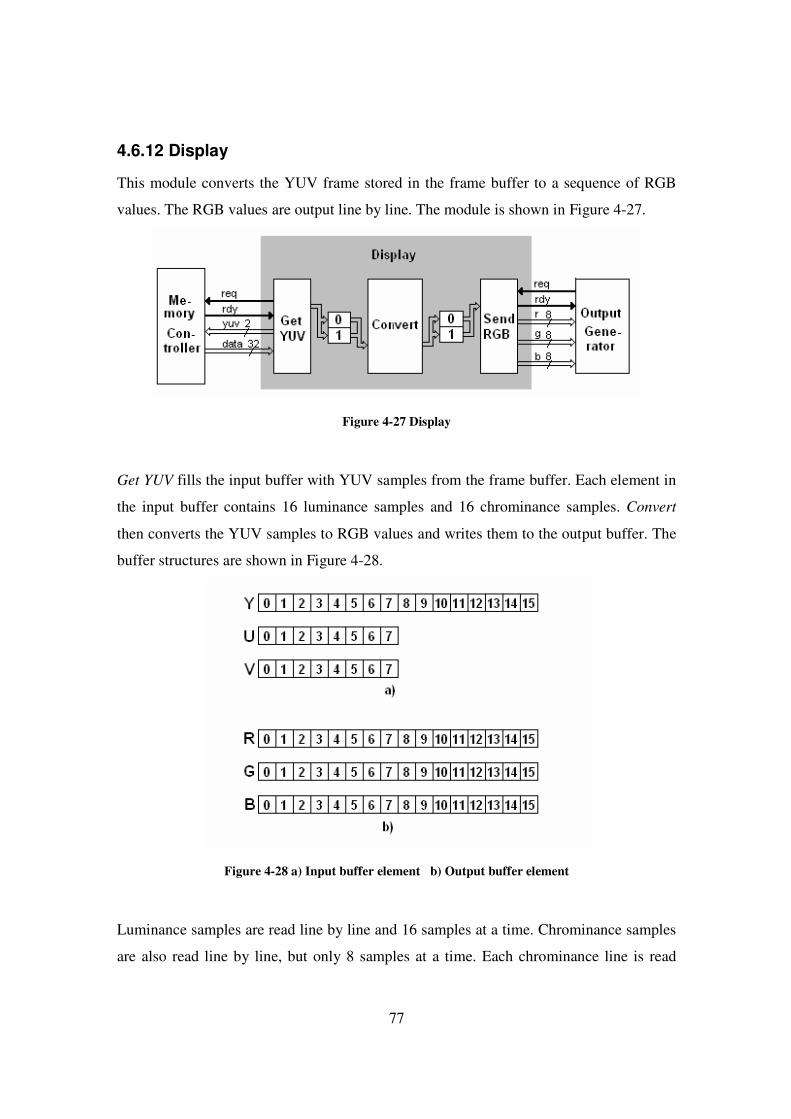
77

4.6.12 Display

This module converts the YUV frame stored in the frame buffer to a sequence of RGB

values. The RGB values are output line by line. The module is shown in Figure 4-27.

Figure 4-27 Display

Get YUV fills the input buffer with YUV samples from the frame buffer. Each element in

the input buffer contains 16 luminance samples and 16 chrominance samples. Convert

then converts the YUV samples to RGB values and writes them to the output buffer. The

buffer structures are shown in Figure 4-28.

Figure 4-28 a) Input buffer element b) Output buffer element

Luminance samples are read line by line and 16 samples at a time. Chrominance samples

are also read line by line, but only 8 samples at a time. Each chrominance line is read

78

twice so that the chrominance samples correspond to the luminance samples. The

Memory Controller handles access to the frame buffer and ensures that the proper

samples are transferred to the Display module.

Send RGB sends the RGB samples to the Output Generator module one pixel at a time.

4.6.12.1 YUV to RGB

The conversion formula is repeated here for readability.

( ) ( )( ) ( ) ( )( ) ( )128596.116164.1

128391.0128813.016164.1128018.216164.1

−+−=−−−−−=−+−=

vyr

uvyg

uyb

The conversion is done using fixed point arithmetic and predefined lookup tables. 13 bits

are used for the fractional part and the following constants are predefined.

Five lookup tables are then predefined.

The conversion of each pixel requires 5 lookups, 4 additions and 3 shifts.

#define SCALEBITS_OUT 13 #define FIX_OUT(x) ((uint16_t) ((x) * (1L<<SCALEBITS_OUT) + 0.5)) #define RGB_Y_OUT FIX_OUT(1.164) #define B_U_OUT FIX_OUT(2.018) #define G_U_OUT FIX_OUT(0.391) #define G_V_OUT FIX_OUT(0.813) #define R_V_OUT FIX_OUT(1.596)

for (i = 0; i < 256; i++) { RGB_Y_tab[i]= RGB_Y_OUT * (i - Y_ADD_OUT); B_U_tab[i] = B_U_OUT * (i - U_ADD_OUT); G_U_tab[i] = G_U_OUT * (i - U_ADD_OUT); G_V_tab[i] = G_V_OUT * (i - V_ADD_OUT); R_V_tab[i] = R_V_OUT * (i - V_ADD_OUT);

}

79

The values are clamped to keep them within the range [0; 255].

4.6.13 Output Generator

This module outputs the RGB values to a monitor. The module is shown in Figure 4-29.

Figure 4-29 Output Generator

RGB values are read into a buffer and sub sequentially written to a monitor. Each buffer

element contains the RGB samples of a single pixel. Sync Signal provides the signal that

controls the output rate. valid is asserted when a new output is written. new_line is

asserted to indicate the start of a new line. new_frame is asserted to indicate the end of

the last line.

This module has been been implemented with testing in mind. The output signals need to

be altered for frames to be shown on a display.

b_u = B_U_tab[u]; g_uv = G_U_tab[u] + G_V_tab[v]; r_v = R_V_tab[v]; rgb_y = RGB_Y_tab[y]; b = (rgb_y + b_u) >> SCALEBITS_OUT; g = (rgb_y - g_uv) >> SCALEBITS_OUT; r = (rgb_y + r_v) >> SCALEBITS_OUT;

80

The monitor is part of the testbench and is described in Chapter 5.

81

5 Testing

The decoder has been tested for correctness at the behavioral level. The testbench shown

in Figure 5-1 was used.

Figure 5-1 Testbench

The stimulus generator is the memory holding the MPEG-4 bitstream. The content of the

memory is read from a file holding the bitstream. The format of this file is described in

Section 5.1. The monitor stores the output of the decoder as a sequence of uncompressed

BMP image files. A full description of the BMP file format is included in Appendix D.

Appendix F includes a description of how to compile and simulate the model.

5.1 Bitstream storage

The MPEG-4 bitstream used for testing was stored in a MP4U container file. The file

format is used by XviD developers for testing purposes and has the file extension

“.mp4u”. The initial 4 bytes of the file contains the string “MP4U” and the rest of the file

contains chunks of data. Each chunk of data contains the coded bitstream for a single

VOP. Data chunks are preceded by a 4 byte field, which indicates the size of the data

chunk. The “MP4U” string is used to identify a valid MPEG-4 bitstream container and

the size field enables users to import a fraction of the bitstream at a time. A MP4U

82

container file is used by the stimulus generator to emulate the content of the bitstream

memory.

5.2 Bitstream creation A program “avi2xvid” capable of extracting the MPEG-4 bitstream from an AVI file was

written. The program extracts the MPEG-4 bitstream from any AVI file coded with the

XviD CODEC and stores it in a MP4U container file. Additionally the program was

linked to the original unmodified XviD CODEC so that the bitstream could be decoded.

The XviD CODEC support several colorspace formats for the decoded frames. The

decoded frames were stored as a series of BMP image files in the 24-bit RGB colorspace.

These BMP files were later compared with the decoder output to test the correctness of

the decoder. It is important to note that the RGB values stored in the BMP files were the

direct output of the original unmodified XviD CODEC.

Encoding software VirtualDub 1.5.1 was used to encode AVI files with the XviD

CODEC. The encoder settings are listed in Appendix B.

A brief description of the AVI file format is included in Appendix E.

5.3 Test results VirtualDub was used to generate a test video containing 10 frames coded with a constant

bit rate of 64 Kbps using H.263 quantization and a resolution of 144x176. The first frame

was intra coded and the following 9 frames inter coded. The encoder settings used to

encode the test video is listed in Appendix B. “avi2xvid” was used to extract the

bitstream and the decoded frames from the test video. The generated MP4U container file

was then used in the testbench.

Finally the decoder was used to decode the bitstream and the output compared with the

output of the original XviD CODEC. The comparison was done using simple file

comparison. The output files were identical to the reference files generated by the

83

unmodified XviD CODEC. The test successfully verified the correctness of the

implemented decoder.

5.4 Bandwidth analysis Real-time decoding of QCIF resolution video at 15 fps requires decoding of 9x11 MBs

15 times a second. Each MB requires 6x8x8 coefficients to be processed. The bandwidth

requirements for the image processing modules; Quant, Idct and interpolate are

( ) scoeff. 57024088615119 =×××××

Assuming a clock cycle of 50 ns (20MHz) means that each coefficient in a MB must be

processed in

cyclesclock 350730,35s 570240s 1020 -1-16 ≈=×

Each 8x8 block must be processed within

cyclesclock 22408835 =××

5.5 Synthesis The Tbuffer module was scheduled, and a structural RTL netlist, ready for compilation to

gates, was generated. Additionally the scheduled design was written to a SystemC format

file optimized simulation speed. This file contained a cycle-accurate RTL-netlist and was

used for cycle-accurate simulation of the Tbuffer module in the testbench. The simulation

verified the correctness and synthesizability of the Tbuffer module. This was important

because the internal buffer structure and the interface protocol of the Tbuffer module was

used in most of the other modules.

The Quant module was also synthesized to a structural RTL netlist. A scheduling report

was generated and an analysis of the report showed that 12 clock cycles is used for the

quantization of a single coefficient, without pipelining. This is well within the 35 clock

cycles available.

84

The Idct module was not synthesized. An implementation of the IDCT on a Xilinx Virtex

FPGA is describes in [16]. This implementation uses 16 1D-IDCT hardware modules.

Each 1D-IDCT module has latency of 13 clock cycles at a clock frequency of

approximately 53 MHz. An implementation of the 8x8 IDCT using only a single of these

modules would result in a block latency of

( ) cyclesclock 2081382 =××

This is well within the 2240 clock cycles available.

85

6 Conclusion

An MPEG-4 Simple@L0 compliant decoder has been successfully modeled using

SystemC. The model has been tested for correctness at the behavioral level. The test was

performed by comparing the output of the model with the output of the XviD CODEC.

The rewriting process of converting the XviD CODEC to SystemC proved more time

consuming than originally anticipated. The structural differences of a software codec and

a hardware decoder required a lot of rearranging. XviD handles intra frames and inter

frames using separate functions. These functions had to be merged and integrated into

modules capable of processing both intra and inter frames. Data size and access patterns

also required careful analysis. XviD declares storage for data structures such as the

bitstream, VOP header, MB header, and the reference VOP at the top hierarchical level,

and then passes pointers to access these. In hardware modeling, modules only have

access to their own data. Data defined in other modules must be transferred before it can

be accessed, which introduces additional latency. Declaration of data storage was done

with the aim of minimizing data transfers. Replacing the native C++ data types with bit

width accurate data types required in some cases very careful analysis of their range.

The most time consuming parts of the rewriting process were elimination of pointers,

declaration of data storage and integration of intra and inter functions.

Behavioral modeling requires use of two-way handshake protocols because designs are

not cycle accurate. This made it more difficult to model interfaces because clock accurate

behavior could not be determined before synthesis. Modeling the internal behavior of the

modules was on the other hand simple once the intra and intra parts had been rearranged

into modules.

The decoder was completely modeled and the correctness verified before an attempt was

made to synthesize it. It became apparent that some of the code, although not violating

86

any of the design rules in the Synopsys documentation, was not synthesizable. Sometimes

the synthesis tools would display fatal error messages with no indication about the source

of the problem. Other error messages referred to lines in the code not actually causing the

problem. This made it difficult to identify the source of the problem. Often the only

option was to comment out code until the problem was identified. Although the errors

often turned out to be caused by non-synthesizable code, more time was spent identifying

the problems, rather than fixing them. A better approach would have been to synthesize

each module as they were written. This would have reduced the repeated use of the same

non-synthesizable code in other modules.

One of the benefits of behavioral synthesis is the ability to explore the design space

without having to change the source code significantly. Experimenting with speed, power

and area tradeoffs, for modules critical to overall latency would have been a very

interesting part of the project. However most of the time was spend on making the

modules synthesizable. Using the pipelining tool to improve throughput would also have

been interesting. Image processing is highly repetitive and involves many iterations,

which makes it ideal for pipelining.

The Tbuffer module was successfully synthesized to a structural RTL netlist and

simulated at cycle accurate level. This module was chosen as the first module to be

synthesized, because it is simple and because it uses the input/output buffer structure used

in several other modules. Additionally, the two-way handshake protocol, which is used to

transfer MBs between modules, was used by this module.

Behavioral synthesis schedules operations into clock cycles. This higher level of

abstraction offered by behavioral modeling is definitely useful for modeling algorithms.

However behavioral modeling of interfaces and communication protocols does not offer

the same control as RTL modeling. A process cannot release a shared resource, such as a

data bus, using high impedance signals. In fact only one process is allowed to drive a

signal in behavioral modeling. Combinatorial modules such as multiplexers are not

87

allowed, which means that all modules have an inherent latency of at least one clock

cycle.

Future work on the model may include implementation of an input buffer scheme for

importing the bitstream. Implementation of a DRAM interface for the reference VOP and

the frame buffer memory blocks. Implement a module capable of displaying the decoded

frames on a display. Full synthesis of the decoder to FPGA using the pipeline tool.

It has been very interesting to learn about MPEG-4 and the compression tools included in

the standard. Although not relevant for this project the object-based representation of

audiovisual content adopted by MPEG-4 is also an area that seems very exciting. Greater

understanding and appreciation of the issues involved in block-based DCT compression

methods and valuable experience in behavioral modeling was achieved. Dealing with

coded MPEG-4 data at bit level gave valuable insights into how bitstreams are

constructed.

End of report

89

References

[1] ISO/IEC 14496-2: MPEG-4 Visual Draft International Standard, 2001.

[2] Synopsys. CoCentric SystemC Compiler Behavioral User and Modelling Guide

version2003.06, 2003.

[3] F. Pereira, T. Ebrahimi. The MPEG-4 Book. Prentice Hall, 2002.

[4] Keith Jack. Video demystified. A Handbook for the Digital Engineer. LLH

Publications. 3rd edition. 2001.

[5] Y. Arai, T. Agui, M. Nakajima. A Fast DCT-SQ Scheme for Images. Trans. of

the IEICE.E 71(11):1095. November 1988.

[6] S. Swan. An Introduction to System-Level Modeling in SystemC 2.0. Cadence

Design Systems, Inc. May 2001.

[7] SystemC 2.0 User’s Guide, Open SystemC Initiative (OSCI).

<www.systemc.org>. 2002.

[8] Functional Specification for SystemC 2.0. Open SystemC Initiative (OSCI).

<www.systemc.org>April 2002.

[9] G. Economakos, P. Oikonomakos, I. Panagopoulos, I. Poulakis, G.

Papakonstantinou. Behavioral Synthesis with SystemC. National Technical

University of Athens.

[10] S. Y. Liao. Towards a new Standard for System-Level Design. Advanced

Technology Group, Synopsys, Inc.

[11] A. E. Walsh, M. Bourges-sevenier. MPEG-4 Jump-start. Prentice Hall, 2002.

[12] E. B. van der Tol, E. G. T. Jaspers. Mapping of MPEG-4 decoding on a flexible

architecture platform. Philips Research Lab.

[13] Synopsys. CoCentric System Studio Enables Verification at Multiple Levels of

Abstraction with SystemC. January 2002.

[14] Synopsys. CoCentric SystemC Compiler. 2002.

[15] J. Gerlach, W. Rosenstiel. System Level Design Using the SystemC Modeling

Platform. University of Tubingen, Germany.

90

[16] K. Chaudhary, H. Verma, S. Nag. An Inverse Discrete Cosine Transform (IDCT)

Implementation in Virtex for MPEG Video Applications. Application Note. Xilinx

XAPP208 v.1.1. December, 1999.

[17] Lars Novak, Magnus Svensson. MMS-Building on the success of SMS. Ericsson

Review No. 3, 2001.

[18] Ericsson, Ericsson releases world’s first EMS mobile phone. Press release. 13

August 2001.

Websites:

[19] <www.xvid.org>

[20] <www.systemc.org>

[21] <www.synopsys.com>

[22] <www.msdn.microsoft.com>

[23] <www.3gpp.org>

[24] <labs.divx.com>

91

7 Appendix A

MPEG-4 Background

Earlier standards such as MPEG-1 and MPEG-2 addressed the issue of compression by

representing video as a sequence of rectangular frames. The primary goal of these

standards was efficient compression. The developers of the MPEG-4 standards met for

the first time in September 1993 to identify the requirements of a very low bit-rate coding

solution. It was soon realized that results such as those produced by the LBC (Low Bit-

rate Coding) (later known as the ITU-T H.263) group where close to the optimal using

the traditional block-based, hybrid, DCT/motion-compensation video decoding method.

Objectives

At the time it was believed that significant improvements over the LBC standard using

conventional coding techniques that would justify another standard could not be achieved.

The group felt the need to broaden the objectives of the MPEG-4 standards.

They assessed current and future trends in the world of multimedia and specifically

addressed the issue by observing how audiovisual content was produced, delivered and

consumed.

Traditionally audiovisual content where mostly natural 2D content produced with

cameras and microphones and edited at the production stage. The audiovisual content

would most often be transmitted over a few homogenous networks (ISDN, LAN, Satellite)

using their own representation scheme. Consumption would be passive and the content

pre-composed.

The group anticipated future audiovisual content to include both natural and computer-

generated synthetic elements and produced such that coding and composition is done

separately for individual objects. Delivery would happen across heterogeneous networks

92

with varying bandwidth capabilities using a common representation scheme. Some

degree of composition would happen at the consumption stage allowing information to be

consumed interactively.

These observations resulted in a coding standard which would support content-based

communication, access and manipulation of digital audiovisual data. The aim was to

achieve both high interactivity and better compression ratio. Where as previous standards

viewed video as sequence of rectangular frames the MPEG-4 standards adopted another

approach. An object-based representation of audiovisual content was adopted.

This approach implied building an audiovisual scene from individual object related only

in time and space. This would enable coding of different types of objects using the most

efficient representation of that particular type of object. Object types may include

rectangular objects, arbitrarily shaped objects, music, speech, synthetic objects, text, still

pictures etc. MPEG-4 standards include special synthetic objects such as 2D and 3D

objects and face and body animation objects.

The object-based approach allow coding of multiple concurrent data streams, mixing of

natural and synthetic objects and content based scalability.

For example a user can edit or change certain characteristics of a single object in the

scene by manipulating the bit stream directly without ever having to transcode the

sequence. Scalability implies the ability to select the decode quality or to prioritize

among object in a scene, useful for delivery over heterogeneous network environments.

Early video coding standards where developed with efficient compression in mind and

have been successfully adopted for commercial use including digital broadcasting, VCD,

DVD and digital television to mention a few. The MPEG-4 standard introduces a new

way of representing audiovisual data using an object-based approach, which is similar to

the way humans view the visual world. This approach allows content based access to data

and a level of interactivity not previously seen in conventional coding schemes.

93

XviD

Originally Microsoft developed a MPEG-4 standard compliant codec called Windows

Media Video V3 (WMV). Microsoft’s WMV encoder did not support saving MPEG-4

streams to the AVI file format, forcing users to use Microsoft´s own file format

Advanced Streaming Format (ASF). The ASF file format also restricted users to use

Microsoft´s Windows Media Audio (WMA) encoder codec to save audio streams. These

restrictions lead to the development of Divx;) also known as DivX v3.11 alfa, which was

a hacked illegal version of the original WMV codec. DIVX;) supported saving to AVI

files as well as mp3 audio streams and quickly became very popular.

Its popularity lead the people behind the hacked version to start up new a company

DivXNetworks Inc in May 2000 and development of a legal version of the codec

commenced. This coded would be coded from scratch and began as an open source

project called Project Mayo or OpenDivX. The company eventually started developing a

closed source version of the codec and released it in August 2001 under the name DivX

4.0.

Open source developers from the original Project Mayo project wished to continue an

open source version and started the XviD (DivX spelled backwards) project.

When this project started the latest version was version 0.91 and this version is used for

this project. This version implements the Simple Profile. Current versions of XviD

implement the Advanced Simple Profile.

95

8 Appendix B

8.1 Encoder settings VirtualDub 1.5.1 was used as the encoding software in this project. Table 8-1 lists the

encoder settings. The 2nd column indicates the available settings provided by the

encoding software. The 3rd column indicates the restrictions to these settings by the

Simple@L0. The final column indicates the settings used to encode the test video used

for testing. Empty fields indicate no restrictions.

Setting Range Simple@L0 Test Video Frame rate (fps) �1 Max. 15 15 Encoding mode 1 Pass – CBR

1 Pass – quality 1 Pass – quantizer 2 Pass – 1st pass 2 Pass – 2nd pass ext. 2 Pass – 2nd pass int.

1 Pass - CBR

Bitrate (Kbits/s) �10000 64 64 Motion search precision

0 – None 1 – very low 2 – low 3 – medium 4 – high 5 – very high 6 – ultra high

6 – ultra high

Quantization type H.263 MPEG MPEG-Custom

H.263 H.263

Max. I-frame interval �0 �0 11 Min. I-frame interval �0 �0 11 Luminance masking Disable

Enable Disable

Interlacing Disable Enable

Disable Disable

Min. I-frame quantizer 1-31 1-31 1 Max. I-frame quantizer 1-31 1-31 31 Min. P-frame quantizer 1-31 1-31 1 Max. P-frame quantizer 1-31 1-31 31 Custom intra matrix Disable

Enable Disable Disable

Custom inter matrix Disable Disable Disable

96

Enable Max. bitrate (Kbits/s) �Bitrate �64 Decomp. format 16-bit (HiColor)

24-bit (TrueColor) 24-bit (TrueColor)

Output format 16-bit (HiColor) 24-bit (TrueColor) 32-bit (TrueColor)

24-bit (TrueColor)

Table 8-1 Encoder settings

97

9 Appendix C

VOP Header Table 9-1 lists the data elements included in the VOP header.

Name width Comments vop_start_code 32 000001B6 (Hexadecimal) vop_coding_type 2 VOP coding method. Defined in Table 9-2 modulo_time_base - Consists of a number of consecutive 1 followed by a 0.

The number of 1s indicate the number of seconds elapsed since the last synchronization point

vop_time_increment 1-16 The absolute time increment from the synchronization point marked by modulo_time_base measured in clock ticks

vop_coded 1 When set to 0 no subsequent data exists for the VOP.and the VOP is copied from the reference VOP.

vop_rounding_type 1 Used for proper rounding during interpolation intra_dc_vlc_thr 3 A 3-bit code which is used to switch between two VLCs

for coding of intra DC coefficients. Defined in Table 9-3 quant_type 1 Determines which of the two quantization methods to use. vop_quant 5 An unsigned integer which specifies the absolute

quantizer stepsize to be used for dequantizing the MB until updated by dquant

vop_fcode_forward 3 An unsigned integer used for decoding motion vectors

Table 9-1 - VOP header

vop_coding_type coding method 00 intra-coded (I) 01 predictive-coded (P) 10 bidirectionallly-predictive-coded (B) 11 sprite (S)

Table 9-2 Meaning of vop_coding_type


index meaning of intra_dc_vlc code 0 use Intra DC VLC for entire VOP 000 1 switch to Intra AC VLC at running Qp�13 001 2 switch to Intra AC VLC at running Qp�15 010 3 switch to Intra AC VLC at running Qp�17 011

98

4 switch to Intra AC VLC at running Qp�19 100 5 switch to Intra AC VLC at running Qp�21 101 6 switch to Intra AC VLC at running Qp�23 110 7 use Intra AC VLC for entire VOP 111

Table 9-3 Meaning of intra_dc_vlc_thr


running Qp is the quantization stepsize of the previous MB.

MB Header Table 9-4 lists the data elements included in the MB header.

Name width Comments not_coded 1 When set to 1 no more data exists for the current macroblock

and the macroblock is copied from the reference VOP mcbpc 1-9 A VLC that is used to derive the macroblock type and the

coded block pattern for chrominance acpred_flag 1 When set to 1 AC prediction is used cbpy 1-6 A VLC that is used to derive the coded block pattern for

luminance (Y) dquant 2 A 2-bit code specifies changes to vop_quant. Found only in

INTRA_Q and INTER_Q MBs. The changes are valid for all subsequent MBs. Defined in Table 9-6

dc_scaler* 6 The dc_scaler may be different for luminance and chrominance components.

quant_stepsize* 5 Quantization stepsize.

Table 9-4 MB header


*quant_stepsize and dc_scaler are derived from the VOP header and the MB header and

are not coded in the bitstream.

In addition to the data elements listed in Table 9-4 each MB is associated with a

quantization stepsize called quant_stepsize. quant_stepsize is equivalent to vop_quant

after the changes by dquant have been made.

dc_scaler is derived from quant_stepsize. This is shown in Table 9-5.

99

dc_scaler for quant_stepsize Component 1 to 4 5 to 8 9 to 24 � 25

Luminance 8 2* quant_stepsize quant_stepsize+8 2* quant_stepsize-16 Chrominance 8 (quant_stepsize+13)/2 quant_stepsize-6

Table 9-5 dc_scaler expressed in terms of the quant_stepsize


dquant code value 00 -1 01 -2 10 1 11 2

Table 9-6 dquant codes


101

10 Appendix D

10.1 BMP file format The BMP file format is described next. Only those parts relevant for this project are

described. The Device Independent Bitmap is the format which is used to store bitmaps

in BMP files. A BMP file contains the following structures

� Bitmap file header

� Bitmap info header

� RGB values

The bitmap file header contains information about the BMP file. The bitmap info header

contains information about the bitmap data. The RGB values are the image data. The

structure of the bitmap file header is shown in Table 10-1. All sizes are in byte units.

Name Size Default Comments bfType 2 19778 Always “BM” bfSize 4 - Size of the file in bytes bfReserved1 2 0 Always 0 bfReserved2 2 0 Always 0 bfOffBits 4 54 Offset from beginning of file to image data

Table 10-1 Bitmap file header

The structure of the bitmap info header is shown in Table 10-2.

Name Size Default Comments biSize 4 40 Size of bitmap info header biWidth 4 - Width of image in pixels biHeight 4 - Height of image in pixels biPlanes 2 1 Always 1 biBitCount 2 24 Number of bits per pixel biCompression 4 0 Always 0 (No compression) biSizeImage 4 0 Always 0 (No compression) biXPelsPerMeter 4 0 Horizontal pixels per meter on the target device

(usually set to zero) biYPelsPerMeter 4 0 Vertical pixels per meter on the target device

(usually set to zero) biClrUsed 4 0 Number of colors used in the bitmap. Automatically

calculated when set to 0

102

biClrImportant 4 0 Number of colors that are important for the bitmap. Set to 0 when all colors are important

Table 10-2 Bitmap info header

The image data are stored a row at a time starting from the bottom row. The start of each

row is aligned to the next 4-byte position. Each pixel in a row is represented as a

sequence of B, G, and R values in that order.

103

11 Appendix E

11.1 AVI File format The AVI file is a RIFF file containing mandatory RIFF chunks. The top-level chunk is

the AVI RIFF chunk with a FOURCC of AVI. The AVI RIFF chunk includes two

mandatory list chunks with FOURCC hdrl and movi and an optional index chunk with

FOURCC idx1. The hdrl chunk includes header information about the format of the

included data. The movi chunk contains the actual data, and idx1 is an optional index of

the data. For more information on the RIFF file format readers are referred to [22].

105

12 Appendix F

12.1 File structure The source files are listed in Table 12-1. Module Location Files Comments - mpeg4\ Makefile builds the

decoder - mpeg4\ constants.h constants - mpeg4\ global.h data types - mpeg4\ main.cpp testbench (top-

level) getBits mpeg4\getbits\ getbits.h

getbits.cpp

Demux mpeg4\demux\ demux.h demux.cpp

Scan Prediction

mpeg4\texture\ scan_prediction.h scan_prediction.cpp

Tbuffer mpeg4\texture\ tbuffer.h tbuffer.cpp

Quant mpeg4\texture\ quant.h quant.cpp

Idct mpeg4\texture\ idct.h idct.cpp

MV Prediction mpeg4\motion\ mv_prediction.h mv_prediction.cpp

Mbuffer mpeg4\motion\ mbuffer.h mbuffer.cpp

Interpolate mpeg4\interpolate\ interpolate.h interpolate.cpp

Reconstruct mpeg4\reconstruct\ reconstruct.h reconstruct.cpp

Memory Controller

mpeg4\memory_controller\ memory_controller.h memory_controller.cpp

Display mpeg4\display\ display.h display.cpp

Output Generator

mpeg4\display output_generator.h output_generator.cpp

Memory mpeg4\memory\ memory.h memory.cpp

bitstream

Monitor mpeg4\monitor\ monitor.h monitor.cpp

writes to bmp

Frame Buffer mpeg4\ram\ cur_ram.h cur_ram.cpp

106

Reference VOP

mpeg4\ram\ ref_ram.h ref_ram.cpp

Table 12-1 Source files

Other files are listed in Table 12-2.

File Location Comments

out.mp4u avi2xvid\ MP4U container with the coded

bitstream for the test video

test_video avi2xvid\ The AVI test video

Makefile avi2xvid\ Makefile for avi2xvid

avi2xvid.exe avi2xvid Program

lixvidcore.lib avi2xvid\ XviD static link library

- xvidcore\src\ XviD CODEC source filer

Makefile xvidcore\build\ Make file for XviD CODEC

Table 12-2 Other files

12.2 Simulating the model Build the XviD CODEC by running

>xvidcore\build\generic\configure

>xvidcore\build\generic\make

>xvidcore\build\generic\make install

This will build and install the static link library xvidcore.lib to av2xvid\.

Then build avi2xvid by running

>avi2xvid\make

Then run

>avi2xvid test_video.avi

107

This will create the out.mp4u and the BMP image files in the avi2xvid\frames\ directory.

Copy the out.mp4u to mpeg4\ and run

>mpeg4\make

This will build the MPEG-4 decoder simulation model. Run

>mpeg\decoder 3000000

The parameter is the maximum number of cycles used in the simulation. The model will

now store the decoded frames in mpeg4\frames\ directory. These can be compared with

the frames in avi2xvid\frames\.

High-Level Synthesis of a MPEG-4 Decoder Using SystemC

Documents

Transcript of High-Level Synthesis of a MPEG-4 Decoder Using SystemC