High-Growth Firms: Rising Tide Lifts All Boats

Policy Research Working Paper 8642

High-Growth Firms: Rising Tide Lifts All BoatsFrancesca de NicolaBalázs MuraközyShawn W. Tan

Finance, Competitiveness and Innovation Global Practice November 2018

WPS8642P

ublic

Dis

clos

ure

Aut

horiz

edP

ublic

Dis

clos

ure

Aut

horiz

edP

ublic

Dis

clos

ure

Aut

horiz

edP

ublic

Dis

clos

ure

Aut

horiz

ed

Produced by the Research Support Team

Abstract

The Policy Research Working Paper Series disseminates the findings of work in progress to encourage the exchange of ideas about development issues. An objective of the series is to get the findings out quickly, even if the presentations are less than fully polished. The papers carry the names of the authors and should be cited accordingly. The findings, interpretations, and conclusions expressed in this paper are entirely those of the authors. They do not necessarily represent the views of the International Bank for Reconstruction and Development/World Bank and its affiliated organizations, or those of the Executive Directors of the World Bank or the governments they represent.

Policy Research Working Paper 8642

How do high-growth firms affect the rest of the economy? This paper explores this question using Hungarian adminis-trative microdata. It finds evidence of stronger productivity growth for firms supplying and operating in industries with more high-growth firms. The surge of high-growth

firms’ demand for intermediate inputs could explain this positive vertical spillover. Firms with intermediate produc-tivity levels seem most likely to benefit from this effect. The results hold irrespective of the level of spatial aggregation.

This paper is a product of the Finance, Competitiveness and Innovation Global Practice. It is part of a larger effort by the World Bank to provide open access to its research and make a contribution to development policy discussions around the world. Policy Research Working Papers are also posted on the Web at http://www.worldbank.org/research. The authors may be contacted at [email protected] or [email protected].

High‐Growth Firms: Rising Tide Lifts All Boats*

Francesca de Nicola Balázs Muraközy Shawn W. Tan

The World Bank CERS Hungarian Academy of

Sciences

The World Bank

Keywords: High growth firms, productivity growth, spillovers, vertical linkages, Hungary

JEL‐codes: D24, D57, L26, O12

* The authors would like to thank Alvaro Gonzalez, Arti Grover, and Denis Medvedev, and participants at theauthor’s workshop for the report on High Growth Entrepreneurship and the ECA Chief Economist Seminar for theirhelpful comments. This paper is based on a background paper produced for the upcoming World Bank report onHigh Growth Firms.

2

1 Introduction

Promoting job creation is a policy priority for many governments seeking to create gainful employment

for their growing youth population and create pathways to economic transformation. For their potential

contribution to this goal, high‐growth firms (HGF) – firms with significant ability to rapidly grow

employment – have increasingly attracted the attention of policy makers. Programs catering to these

entities tend to rely on broad policy instruments, similar to those used to support SMEs. See Autio et al.

(2007) and World Bank (2018) for a review of the evidence on these measures from advanced and

developing countries, respectively. Governments in developing countries have scarce resources and

administrative capacity to support entrepreneurship and may be concerned about how much of them to

devote to HGF promotion in the hope of creating jobs. This is, however, is a simplistic way to frame the

issue for policy makers, as HGFs can generate employment but they can also generate spillover benefits

for other firms in the economy.

Much attention in the literature and among policy makers has focused on the benefits generated by

HGFs and how to implement policies to encourage more HGFs. But HGFs also generate externalities and

the net effect on the overall economy is ambiguous. On the one hand, HGFs may exert competitive

pressures on input and output prices, crowding out other firms. They may poach workers from

competitors, put upward pressure on labor and other input costs, or drive output prices down by

exploiting economies of scale. On the other hand, HGFs may generate positive spillovers. HGFs may

develop or possess knowledge of technology, organization or markets that may transfer to other firms

through movement of employees or demonstration. The knowledge transfer is likely to occur over

relatively short distances through face‐to‐face contact with their clients or suppliers or within the labor

market. In addition, HGFs' high demand for inputs may generate opportunities for suppliers to exploit

economies of scale (Javorcik, 2004), and/or facilitate technology upgrading. Because of their advanced

technology, HGFs may sell high‐quality or innovative inputs, benefitting downstream firms using that

input. Assessing whether positive or negative spillovers prevail is the empirical question we explore in

this paper.

We rely on detailed firm‐level administrative data from Hungary and exploit regional and time variation

in the share of HGFs to infer their connection with the performance of other related firms. We focus on

vertical spillovers and use the 2‐digit industry input‐output matrix to determine the share of HGFs in

upstream and downstream industries. This focus is motivated by the fact that the related literature on

MNE spillovers documents stronger evidence for vertical or intra‐industry spillovers rather than

horizontal ones. We also consider a more refined measure of horizontal spillovers, or intra‐industry

spillovers, where we measure the share of HGFs in the firm’s 2‐digit industry and county, omitting the

firms' own 4‐digit industry.

In our empirical strategy, we carefully adapt the methods in the FDI spillover literature to the HGF

environment. From a technical point of view, a crucial difference is that the HGF phase is more transient

than the FDI one, which, in turn, limits the application of fixed effects methodologies employed in the

latter literature. We handle this issue by regressing log differences on the level of spillover measures

and firm controls. Relatedly, in contrast with the FDI case, the share of HGFs is mechanistically linked to

the growth distribution, generating challenges discussed in the peer effect literature (see, for example,

3

Angrist 2014). We handle this problem by excluding firms in the same narrowly defined (4‐digit) industry

from the calculation of spillover measures. A third issue is that unobserved demand shocks can

confound the relationship between high growth and productivity increase in related industries. While

we employ a large set of fixed effects to control for these shocks, our results can be interpreted as

correlation between high share of HGFs and productivity growth rather than a causal relationship.

We find evidence consistent with positive spillovers. Rather than attracting workers from or reducing

profits of non‐HGFs, HGFs’ presence seems to be linked to improvements in productivity, income and

employment of other local firms. Among them, suppliers of HGFs appear to benefit most from their

presence. Effects are heterogeneous: firms with medium productivity levels appear to gain most from

HGFs’ presence in downstream sectors. This may be explained by the low absorptive capacity of low

productivity firms, and the looser relations between local markets and the most productive firms.

We contribute to different strands of the literature. First, we build on and add to the literature on the

role of entrepreneurship in development. This literature emphasizes that while entrepreneurship in

general is a key determinant of economic growth and employment (Carree and Thurik, 2010), a subset

of entrepreneurs, often called high‐impact entrepreneurs, contributes disproportionately to

employment and economic growth (Autio et al., 2007). The literature also emphasizes key functions of

high‐impact entrepreneurs: they apply existing knowledge in innovative ways (Audretch, 2005) and

operate where demand or supply characteristics were unknown (Ács, 2010). Both activities yield new

knowledge, at least locally, thus having the potential to create externalities. Our paper contributes to

better understanding the externalities generated by such entrepreneurs.

The entrepreneurship literature is partly motivated by the literature on the role of industrial policy in

development. Hausman and Rodrik (2003) interpret development as a process of discovering a country’s

cost structure when producing different goods. In general, this type of self‐discovery is under‐provided

because of public good problems (Rodrik, 2005). High impact entrepreneurs can play a key part in

providing such self‐discovery, as they are likely to investigate production functions and generate

externalities via learning by doing for firms in similar activities. Furthermore, our analysis of inter‐

industry spillover effects resulting from HGFs may also inform industrial policy (Harrison and Rodríguez‐

Clare, 2010).

Second, we expand the growing literature on HGFs. So far, the debate has focused on the identification

of these fast‐growing firms and their characteristics. HGFs tend to be more productive, younger,

engaged in scientific R&D and computer programming, but are not concentrated in any given sector

(Coad et at, 2014 and OECD, 2016). However, to the best of our knowledge, the literature has not yet

investigated the impact of HGFs on other firms. This paper aims to fill this gap.

Third, we extend the productivity spillover literature. This literature has often found positive backward

spillovers (see for example, Görg and Greenaway (2004) for a summary of the literature on spillover

effects from foreign firms). Other studies show that positive spillovers may result from intentional or

non‐intentional technology transfer to suppliers from higher quality or productivity requirements

(Blalock and Gertler, 2008), or from access to a higher quality, larger variety or lower priced pool of

inputs (Javorcik, 2004). We contribute to this literature by investigating a different source of spillovers.

We also discuss and propose solutions for new methodological challenges which emanate from the

4

more transient nature of the HGF phase relative to FDI. This contributes to the generalizability of the FDI

spillover methodology to other problems.

The paper is organized as follows. Section 2 describes the data used, the construction of the main

variables of interest and the empirical strategy. Section 3 presents our results. Finally, Section 4

summarizes the evidence presented.

2 Data and Empirical Strategy

2.1 Data

The primary data set is firm level corporate income tax statements during the period 1998‐2014 from

the Hungarian National Tax Authority (NAV). The data set has almost universal coverage as it covers all

firms that require double‐entry bookkeeping.2 The sample includes more than 95 percent of

employment and value added of the business sector and about 55 percent of the full economy in terms

of GDP. The data set includes information on a wide range of matters such as ownership, financial

information, employment, and industry at the NACE 4‐digit code level and the location of their

headquarters. The Centre for Economic and Regional Studies, Hungarian Academy of Science (CERS‐HAS)

extensively cleaned and harmonized the data.

Given the scope of our analysis, we restrict the data in several ways. First, we exclude non‐profit

organizations. Second, we drop firms that operate either in agriculture or in the non‐market service

sectors of the economy.3 Third, we drop all firm‐year observations with fewer than 5 employees.4

Finally, we drop all firm‐year observations with missing, negative or zero employment, turnover,

material cost, capital or value added. As we will discuss in detail in section 2.3, our regression will be run

for 3‐year intervals, which further reduces the number of observations. We also restrict the sample to

surviving firms, given our primary interest in TFP change. Finally, we exclude firms which operate in the

capital, Budapest.5 Our final regression sample consists of more than 140,000 firm‐year observations.6

The data include the most important balance sheet items. Nominal variables were deflated by the

appropriate deflators from Eurostat. We rely on two proxies of productivity. First, labor productivity is

value added over employment. Second, we estimate total factor productivity (TFP) using the semi‐

2 Double‐entry bookkeeping system is an accounting system where every entry has a corresponding entry in a different account. For example, a cash purchase of equipment will appear as a credit on the cash account and a debit on the equipment/capital account. Only sole traders and very small firms are not required to use double‐entry bookkeeping in Hungary. 3 Non‐market services sectors are sectors 53, 58, 75, 84 to 94, and 96 to 99, based on NACE rev 2. 4 We do this to avoid overestimating the incidence of HGFs. Besides, these micro‐sized firms are likely to include individual entrepreneurs who operate a formal firm to reduce their tax burden (Semjén et al., 2009), and many small firms are likely to underreport their sales, earnings and wages paid (Tonin, 2011). 5 We do this for two reasons. First, many larger firms register their headquarters in Budapest even though most of their activities are conducted elsewhere. Second, Budapest, where 20% is a very large geographic entities compared to other counties or microregions, represents an outlier. Our results are robust to including Budapest in the sample. 6 The full sample includes a total of 1.7 million observations for our regression years (1998, 2001, 2004, 2007, 2009, 2011); 320,000 firms have at least 5 employees and 260,000 firms are observable for at least 3 years. From these, we have all the variables to estimate TFP for 210,000, from which we exclude 70,000 because they operate in Budapest.

5

parametric methods in Ackerberg et al. (2015) but will also present results based on other methods

(Wooldridge, 2008), and with fixed effects to check for robustness. These measures are proxies for

revenue productivity, which depends both on physical productivity and markups.7 The dependent

variables in our regressions are 3‐year changes in these productivity measures, employment, sales,

average wage and return on assets (ROA). We winsorize these long differences at the 5th and 95th

percentiles of their distribution, calculated separately for each 2‐digit industry‐year combination.

As for the construction of our main explanatory variable, multiple definitions for HGFs exist in the

literature. A key difference between these methods is whether they rely (i) exclusively on relative

growth rates or (ii) on absolute growth. The former approach tends to identify HGFs as mostly small

firms, while the latter provides a less skewed identification. As all theoretical spillover channels – either

via vertical linkages or the labor market – are likely to be stronger when they originate from larger firms,

the latter measure is more likely to capture these externalities. Hence, that is our preferred approach.

Specifically, we choose to identify HGFs based on the Birch index (Birch, 1981), computed for all firms

with at least 5 employees in year 𝑡:

𝐵𝑖𝑟𝑐ℎ 𝑒𝑚𝑝 𝑒𝑚𝑝𝑒𝑚𝑝

𝑒𝑚𝑝

We rank firms according to their 𝐵𝑖𝑟𝑐ℎ values for each year and classify a firm as HGF if the Birch index

is above the 95th percentile in that year. The constant and absolute threshold generates variation across

industries, regions and years.

As a robustness check, we will estimate the regressions with the OECD definition of HGFs whereby a firm

is high‐growth if it employs at least 5 employees at the beginning of the period and has an annualized

growth rate of employment of at least 20 percent for a period of 3 years (OECD, 2010).

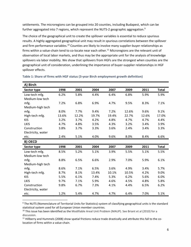
By definition, the share of Birch‐firms is 5 percent for the full sample in each year. There are some

differences across industries, with the most HGFs in high‐tech manufacturing industries.8 The OECD

definition shows similar patterns across industries, but by construction it also varies across years,

following the macro cycle (see Table 1).

Importantly, the data set allows us to exploit the detailed geographical information of each firm. The

data on the municipality of the firms’ headquarters are used to construct our spillover measures.

Municipalities are the smallest geographical unit of measurement in Hungary: they can be aggregated

up to 174 microregions, where each microregion tends to include one city and the neighboring smaller

7 In spite of the conceptual differences between TFPR and TFPQ, Foster et al. (2017) use US data to show that these measures are highly correlated, have similar relationships with growth and survival, and show similar dispersion. These results cast doubt on the interpretation of TFPR as a proxy for distortions as in the Hsieh and Klenow (2009) framework. 8 We rely on Eurostat’s indicators on high‐tech industry and knowledge‐intensive services. Manufacturing industries are grouped in four categories: high‐tech, medium‐high‐tech, medium‐low‐tech and low tech. Services are organized in knowledge‐intensive services and other services.

6

settlements. The microregions can be grouped into 20 counties, including Budapest, which can be

further aggregated into 7 regions, which represent the NUTS‐2 geographic aggregation.9

The choice of the geographical unit to create the spillover variables is essential to reduce spurious

results. A highly aggregated geographical unit may result in spurious correlations between the spillover

and firm performance variables.10 Counties are likely to involve many supplier‐buyer relationships as

firms within a value‐chain tend to co‐locate near each other.11 Microregions are the relevant unit of

observation of local labor markets, and thus may be the appropriate unit for the analysis of knowledge

spillovers via labor mobility. We show that spillovers from HGFs are the strongest when counties are the

geographical unit of consideration, underlining the importance of buyer‐supplier relationships in HGF

spillover effects.

Table 1: Share of firms with HGF status (3‐year Birch employment growth definition)

A) Birch

Sector type 1998 2001 2004 2007 2009 2011 Total

Low‐tech mfg. 6.2% 5.8% 4.4% 6.4% 6.8% 5.9% 5.9% Medium‐low tech mfg. 7.2% 6.8% 6.9% 4.7% 9.5% 8.3% 7.1% Medium‐high tech mfg. 8.0% 7.7% 9.4% 7.2% 12.6% 9.6% 9.1% High‐tech mfg. 13.6% 12.2% 19.7% 19.4% 22.7% 12.6% 17.0% KIS 3.2% 3.7% 4.2% 4.8% 4.7% 4.7% 4.4% LKIS 4.7% 4.8% 3.5% 4.3% 3.2% 3.4% 3.9% Construction 3.8% 3.7% 3.3% 3.6% 2.4% 3.4% 3.3% Electricity, water etc. 2.4% 5.1% 4.0% 9.6% 8.0% 8.4% 6.6%

B) OECD

Sector type 1998 2001 2004 2007 2009 2011 Total

Low‐tech mfg. 8.5% 5.2% 5.1% 3.9% 5.5% 5.1% 5.5% Medium‐low tech mfg. 8.8% 6.5% 6.6% 2.9% 7.0% 5.9% 6.1% Medium‐high tech mfg. 8.6% 7.1% 6.5% 3.6% 4.9% 3.4% 5.7% High‐tech mfg. 8.7% 8.1% 13.4% 10.1% 10.5% 4.2% 9.0% KIS 5.5% 6.1% 7.4% 5.3% 6.2% 5.6% 6.0% LKIS 9.7% 7.1% 5.9% 4.6% 4.5% 4.8% 5.8% Construction 9.8% 6.7% 7.3% 4.1% 4.4% 6.5% 6.2% Electricity, water etc. 1.2% 5.4% 4.7% 4.7% 6.4% 7.0% 5.1%

9 The NUTS (Nomenclature of Territorial Units for Statistics) system of classifying geographical units is the standard statistical system used for all European Union member countries. 10 This issue has been identified as the Modifiable Areal Unit Problem (MAUP). See Briant et al (2010) for a discussion. 11 Hillberry and Hummels (2008) show spatial frictions reduce trade drastically and attribute this fall to the co‐location of firms within a value‐chain.

7

Note: This table shows the share of HGFs (according to the 3‐year Birch and OECD definitions, based on employment) in the regression sample. KIS stands for Knowledge Intensive Services, and LKIS for Less Knowledge Intensive Services. Sector types are defined based on the Eurostat definition.

2.2 Spillover measures

HGFs may affect the rest of the economy through direct and indirect channels. They may affect firms

that buy from and sell to them, but they may also impact firms that are not directly linked to them but

operate in the same sector.

Let 𝐻𝑆 be the share of HGFs in (2‐digit) industry 𝑗, region (county or microregion) 𝑟, and year 𝑡, it

accounts for the firms with at least 5 employees and an HGF phase starting in year 𝑡, 𝑡 1 or 𝑡 2 :12

𝐻𝑆∑ 𝐻𝐺𝐹∈

𝑁

where 𝑁 is the number of firms in industry 𝑗 in region (county or microregion) 𝑟 and year 𝑡, and 𝐻𝐺𝐹

is an indicator variable that equals 1 if firm i is a HGF.

The upstream (forward) and downstream (backward) measures are based on the average share of HGFs

in supplier and buyer industries in the region, weighted by the volume of intermediate‐good flows

across other industries. Importantly, when calculating these measures for a given firm, we omit said

firm’s 2‐digit industry from the computation to capture only genuine inter‐industry spillovers. Buyer‐

seller connections are identified using information from the 2‐digit (symmetric harmonized) input‐

output matrices for Hungary provided by the OECD:13

𝑈𝑝𝑠𝑡𝑟𝑒𝑎𝑚 𝐻𝐺𝐹 𝛼 𝐻𝑆

and

𝐷𝑜𝑤𝑛𝑠𝑡𝑟𝑒𝑎𝑚 𝐻𝐺𝐹 𝛼 𝐻𝑆

where 𝛼 are the normalized coefficients from the symmetric input‐output matrix representing

(domestic) intermediate good flows from industry 𝑚 to 𝑗.

We also control for intra‐industry spillovers by calculating the share of HGFs in the firms’ 2‐digit

industry; using data on all entities with the same 2‐digit code, save for the ones that belong to the firm’s

own 4‐digit industry14 (denoted by 𝑔). Thus, this measure is calculated as:

12 For consistency with the regression sample, we calculate the spillover measures based on the subsample of firms with at least 5 employees. 13 Source: http://stats.oecd.org/Index.aspx?DataSetCode=IOTS. These tables are available only between 2000‐2011, so we have used the 2011 weights for the years after 2011 and the 2000 weights for the years before 2000. 14 The sub‐industry is narrowly defined as it describes one specific economic activity. An example is subindustry 10.11, the processing and preserving of meat. The second measure is the share of HGFs in the firm’s industry defined as the 2‐digit NACE code. The industry is more broadly defined as it captures many economic activities. Using the same example, the processing and preserving of meat will be grouped together with production of meat products under industry 10, manufacture of food products.

8

𝐼𝑛𝑡𝑟𝑎 𝑖𝑛𝑑𝑢𝑠𝑡𝑟𝑦 𝐻𝐺𝐹∑ 𝐻𝐺𝐹∈ ∑ 𝐻𝐺𝐹∈

𝑁 𝑁

All these spillover variables contain extreme values, mainly because of some firms' small size. To prevent

such outliers driving the results, we censor values at 15% for all spillover measures.15

Note that 𝐼𝑛𝑡𝑟𝑎 𝑖𝑛𝑑𝑢𝑠𝑡𝑟𝑦 𝐻𝐺𝐹 is very close to the `traditional’ horizontal HGF measure, as

defined in, for example, Javorcik (2004). The difference is that we omit the firm’s 4‐ digit industry, to

avoid generating spurious correlation. If all firms – including HGFs – are in the sample, then the high

growth of the HGF will show up both in the HGF measure and on the left‐hand side. Omitting HGFs from

the regressions would introduce endogenous selection based on the dependent variable.16

Nevertheless, re‐running the regressions with the traditional horizontal measure yields similar results.17

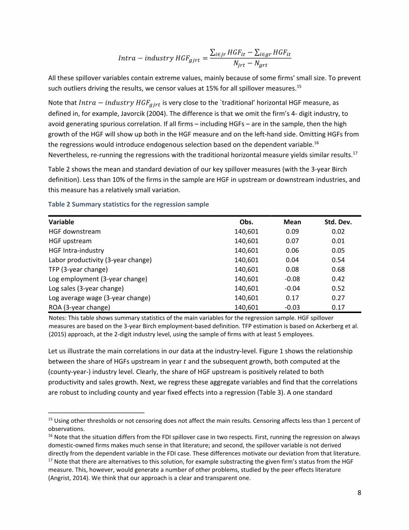
Table 2 shows the mean and standard deviation of our key spillover measures (with the 3‐year Birch

definition). Less than 10% of the firms in the sample are HGF in upstream or downstream industries, and

this measure has a relatively small variation.

Table 2 Summary statistics for the regression sample

Variable Obs. Mean Std. Dev.

HGF downstream 140,601 0.09 0.02

HGF upstream 140,601 0.07 0.01

HGF Intra‐industry 140,601 0.06 0.05

Labor productivity (3‐year change) 140,601 0.04 0.54

TFP (3‐year change) 140,601 0.08 0.68

Log employment (3‐year change) 140,601 ‐0.08 0.42

Log sales (3‐year change) 140,601 ‐0.04 0.52

Log average wage (3‐year change) 140,601 0.17 0.27

ROA (3‐year change) 140,601 ‐0.03 0.17

Notes: This table shows summary statistics of the main variables for the regression sample. HGF spillover measures are based on the 3‐year Birch employment‐based definition. TFP estimation is based on Ackerberg et al. (2015) approach, at the 2‐digit industry level, using the sample of firms with at least 5 employees.

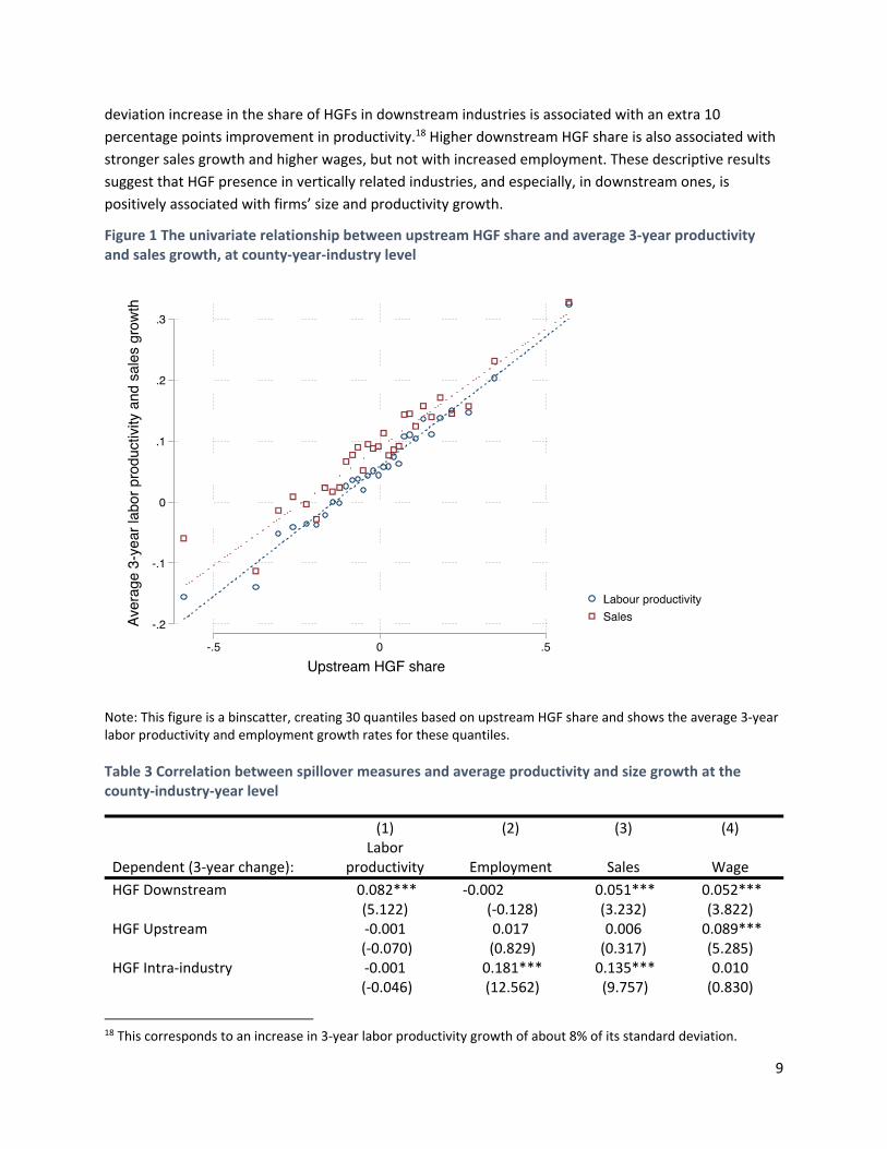
Let us illustrate the main correlations in our data at the industry‐level. Figure 1 shows the relationship

between the share of HGFs upstream in year 𝑡 and the subsequent growth, both computed at the

(county‐year‐) industry level. Clearly, the share of HGF upstream is positively related to both

productivity and sales growth. Next, we regress these aggregate variables and find that the correlations

are robust to including county and year fixed effects into a regression (Table 3). A one standard

15 Using other thresholds or not censoring does not affect the main results. Censoring affects less than 1 percent of observations. 16 Note that the situation differs from the FDI spillover case in two respects. First, running the regression on always domestic‐owned firms makes much sense in that literature; and second, the spillover variable is not derived directly from the dependent variable in the FDI case. These differences motivate our deviation from that literature. 17 Note that there are alternatives to this solution, for example substracting the given firm’s status from the HGF measure. This, however, would generate a number of other problems, studied by the peer effects literature (Angrist, 2014). We think that our approach is a clear and transparent one.

9

deviation increase in the share of HGFs in downstream industries is associated with an extra 10

percentage points improvement in productivity.18 Higher downstream HGF share is also associated with

stronger sales growth and higher wages, but not with increased employment. These descriptive results

suggest that HGF presence in vertically related industries, and especially, in downstream ones, is

positively associated with firms’ size and productivity growth.

Figure 1 The univariate relationship between upstream HGF share and average 3‐year productivity and sales growth, at county‐year‐industry level

Note: This figure is a binscatter, creating 30 quantiles based on upstream HGF share and shows the average 3‐year labor productivity and employment growth rates for these quantiles.

Table 3 Correlation between spillover measures and average productivity and size growth at the county‐industry‐year level

(1) (2) (3) (4)

Dependent (3‐year change): Labor

productivity Employment Sales Wage

HGF Downstream 0.082*** ‐0.002 0.051*** 0.052***

(5.122) (‐0.128) (3.232) (3.822) HGF Upstream ‐0.001 0.017 0.006 0.089***

(‐0.070) (0.829) (0.317) (5.285) HGF Intra‐industry ‐0.001 0.181*** 0.135*** 0.010

(‐0.046) (12.562) (9.757) (0.830)

18 This corresponds to an increase in 3‐year labor productivity growth of about 8% of its standard deviation.

10

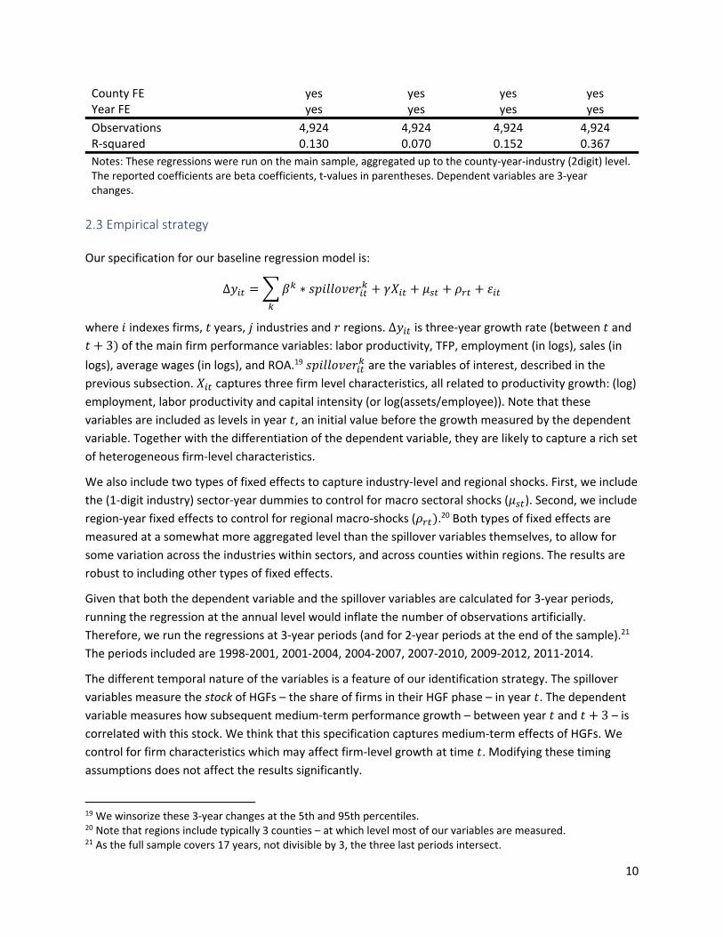
County FE yes yes yes yes Year FE yes yes yes yes

Observations 4,924 4,924 4,924 4,924 R‐squared 0.130 0.070 0.152 0.367

Notes: These regressions were run on the main sample, aggregated up to the county‐year‐industry (2digit) level. The reported coefficients are beta coefficients, t‐values in parentheses. Dependent variables are 3‐year changes.

2.3 Empirical strategy

Our specification for our baseline regression model is:

Δ𝑦 𝛽 ∗ 𝑠𝑝𝑖𝑙𝑙𝑜𝑣𝑒𝑟 𝛾𝑋 𝜇 𝜌 𝜀

where 𝑖 indexes firms, 𝑡 years, 𝑗 industries and 𝑟 regions. Δ𝑦 is three‐year growth rate (between 𝑡 and 𝑡 3 of the main firm performance variables: labor productivity, TFP, employment (in logs), sales (in

logs), average wages (in logs), and ROA.19 𝑠𝑝𝑖𝑙𝑙𝑜𝑣𝑒𝑟 are the variables of interest, described in the

previous subsection. 𝑋 captures three firm level characteristics, all related to productivity growth: (log)

employment, labor productivity and capital intensity (or log(assets/employee)). Note that these

variables are included as levels in year 𝑡, an initial value before the growth measured by the dependent

variable. Together with the differentiation of the dependent variable, they are likely to capture a rich set

of heterogeneous firm‐level characteristics.

We also include two types of fixed effects to capture industry‐level and regional shocks. First, we include

the (1‐digit industry) sector‐year dummies to control for macro sectoral shocks (𝜇 ). Second, we include

region‐year fixed effects to control for regional macro‐shocks (𝜌 .20 Both types of fixed effects are

measured at a somewhat more aggregated level than the spillover variables themselves, to allow for

some variation across the industries within sectors, and across counties within regions. The results are

robust to including other types of fixed effects.

Given that both the dependent variable and the spillover variables are calculated for 3‐year periods,

running the regression at the annual level would inflate the number of observations artificially.

Therefore, we run the regressions at 3‐year periods (and for 2‐year periods at the end of the sample).21

The periods included are 1998‐2001, 2001‐2004, 2004‐2007, 2007‐2010, 2009‐2012, 2011‐2014.

The different temporal nature of the variables is a feature of our identification strategy. The spillover

variables measure the stock of HGFs – the share of firms in their HGF phase – in year 𝑡. The dependent variable measures how subsequent medium‐term performance growth – between year 𝑡 and 𝑡 3 – is correlated with this stock. We think that this specification captures medium‐term effects of HGFs. We

control for firm characteristics which may affect firm‐level growth at time 𝑡. Modifying these timing

assumptions does not affect the results significantly.

19 We winsorize these 3‐year changes at the 5th and 95th percentiles. 20 Note that regions include typically 3 counties – at which level most of our variables are measured. 21 As the full sample covers 17 years, not divisible by 3, the three last periods intersect.

11

Our identification strategy relies on variation from three main sources: geographic variation within

regions, industry variation within sectors and time variation (and the interactions of these variables). We

show that the results are robust to alternative specification. Across‐industry cross‐sectional variation is

necessary for our results. Our results are mainly driven by the stronger productivity growth in industries

vertically related to industries with more HGFs. This is a consequence of several factors. First, there is

limited variation of links in input‐output tables and HGF shares in 2‐digit industries. Second, many

periods are involved when measuring the dependent and the spillover variables. The dependent variable

captures firm growth between periods 𝑡 and 𝑡 3, which depends on changes during this period, including firms starting their high growth period in any of these years.22 The explanatory variables

consider firms which start their high growth period between 𝑡 2 and 𝑡. Consequently, in the empirical

specification one ‘year’ observation consists of changes across 5‐6 years, even not considering delayed

effects of high growth phases. Useful time variation is quite limited.

Clarifying our identification strategy, we compare it to the usual method employed in the FDI spillovers

literature. From a technical point of view, an important difference between the two empirical exercises

is that HGF status is much more transient than foreign ownership: most firms which become foreign

owned remain in that state. As a result, in typical FDI‐spillover equations (e.g. Javorcik, 2004), the

dependent variable is the level of productivity and the equation is estimated with firm fixed effects. This

method is less appropriate when the variable of interest is less persistent, as in the case of HGF status. It

is more intuitive in our setting to check whether productivity growth is higher when more firms are

experiencing an HGF phase in vertically related industries. Note that, similarly to the level‐fixed effects

specification, differencing the dependent variable also filters out time‐invariant firm characteristics.

A second issue with applying the methodology of the FDI spillover literature to measuring HGF spillovers

is that any kind of horizontal measure of HGFs will include the firm itself: if our firm is an HGF, the share

of HGFs in its industry will be automatically higher. The more disaggregated the data, the larger is this

problem. This issue is easily handled in the FDI spillover literature by running the regression only on the

subsample of always domestic firms. This, however, is less of an option in the HGF case, because

restricting the sample to non‐HGFs would lead to the endogenous exclusion of firms with the strongest

growth performance. We will handle this issue in two ways. First, we exclude horizontal spillovers from

our regressions and include different industry fixed effects. Second, we exclude the firm’s 4‐digit

industry from the intra‐industry measure, as indicated above.23

In summary, our identification strategy attempts to use sensible timing assumptions together with a set

of fixed effects. Still, our results are best interpreted as correlations: productivity growth in industries

which supply industries with more HGFs. It is possible that there are unobserved industry

characteristics, which may partly drive this correlation. Also, reverse causality is possible: stronger

productivity growth of suppliers may help their buyers to grow rapidly. Given that regressions aimed at

22 Consider firms that start their high growth phase in T+2, which may clearly affect firm growth between t and t+3. These firms will even be considered HGFs in t+5. 23 One can generate horizontal measures by excluding the firm itself from the regression, following the peer effects literature. However, this also introduces an automatic negative correlation between the horizontal variable and the firm’s performance. Our results are robust to including such horizontal variables.

12

predicting HGF status usually have a low explanatory power, it is unlikely that one can find credible

instruments for regional HGF presence. Consequently, we find our strategy a relatively transparent and

credible way to document the correlation between HGFs and productivity growth in related industries.

3 Results

3.1 Main firm‐level regression results

Our main results are reported in

Table 4. First, the top panel reports the positive relation between productivity growth and HGF share in

vertically related industries. A one‐standard‐deviation increase in HGF share in downstream (buyer)

industries is associated with about 4‐5 percent of a standard deviation increase in labor productivity and

TFP growth. These relationships are significant also from an economic perspective, representing about a

2.5 percentage points additional productivity growth in three years. The impact from HGFs in upstream

(seller) industries is also positive but significant only for labor productivity. Additionally, we find

evidence consistent with the existence of vertical spillovers. The coefficient on the share of HGFs in

same industry is again positive and significant, albeit smaller in economic terms. The results are robust

to two alternative methodologies to measure aggregate productivity (fixed effects and Wooldridge

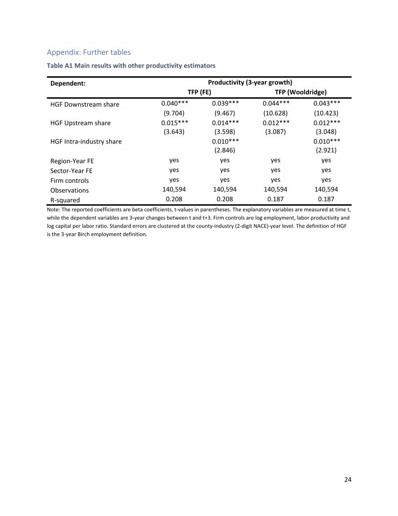
(2008) estimator) (Table A1).

Second, the middle panel examines whether productivity growth is related with firm growth. The

presence of HGFs in downstream industries is associated with higher sales growth, but no extra growth

in employment. This is consistent with HGFs generating additional demand, which may drive the

premium in productivity growth. We do not find similar effects for HGFs in upstream industries. Also,

there is weak evidence for a positive relationship between HGF share in the industry and firm growth.

Third, the bottom panel reports how potential productivity gains are related to income of the two key

shareholders of firms: employees (through higher wages) and owners (through higher ROA). A

comparable increase in wages and ROA is observed when the share of HGF in buyer industries grows.

This similar magnitude reflects different impacts, due to differences in levels of the dependent variables.

The wage effect is small, corresponding to about 0.25 percentage point additional wage growth in 3

years. The ROA effect is more significant, representing nearly an additional 0.4 percentage point

increase in ROA. Taken together, the results suggest that the HGF presence in buyer industries is

associated with higher productivity and stronger sales growth, which seem to benefit workers and, to a

larger extent, owners. This is consistent with backward productivity spillovers from the higher demand

of HGFs.

We also find positive association between HGFs in the same 2‐digit industry, probably due to the

presence of demand effects. We only find weak association between HGF in upstream industries and

productivity growth. The results are robust to using alternative definitions for HGFs (

13

Table A2). A methodological lesson is that multicollinearity is not an extremely serious issue in our case:

the point

estimates of the backward and forward measures do not change much when we include the 2‐digit

variable.24 Similarly, including the three variables sequentially yields consistent point estimates.

Consequently, we include all three variables in the different specifications.

Table 4 Main regression results

Dependent: Productivity (3‐year growth) Labor productivity TFP

HGF Downstream share 0.044*** 0.043*** 0.053*** 0.051*** (10.207) (9.969) (9.184) (8.944)

HGF Upstream share 0.014*** 0.014*** 0.008 0.007 (3.398) (3.360) (1.334) (1.281)

HGF intra‐industry share

0.010***

0.020*** (2.927)

(5.028)

Region‐year FE yes yes yes yes Sector‐year FE yes yes yes yes Firm controls yes yes yes yes Observations 140,594 140,594 140,594 140,594 R‐squared 0.216 0.216 0.170 0.170

Dependent: Size (3‐year growth) Employment (ln) Sales (ln)

HGF Downstream share 0.002 0.001 0.028*** 0.028*** (0.467) (0.306) (5.628) (5.604)

HGF Upstream share 0.004 0.003 0.013** 0.013**

(0.850) (0.793) (2.555) (2.546) HGF intra‐industry share 0.012*** 0.002

(3.475) (0.454) Region‐Year FE yes yes yes yes Sector‐Year FE yes yes yes yes Firm controls yes yes yes yes Observations 140,594 140,594 140,594 140,594 R‐squared 0.084 0.084 0.069 0.069

Dependent: Income (3‐year growth) Average wage (ln) ROA

HGF Downstream share 0.026*** 0.027*** 0.020*** 0.019***

(5.338) (5.616) (4.131) (3.920) HGF Upstream share 0.011** 0.011** 0.004 0.003

(1.981) (2.069) (0.866) (0.803) HGF intra‐industry share ‐0.017*** 0.015***

(‐4.538) (4.175) Region‐Year FE yes yes yes yes Sector‐Year FE yes yes yes yes Firm controls yes yes yes yes Observations 140,594 140,594 140,594 140,594 R‐squared 0.161 0.161 0.095 0.095

24 A reason for this is that the same sectors are omitted from the uptream and downstream measures.

14

Note: The reported coefficients are beta coefficients, t‐values in parentheses. The explanatory variables are measured at time t, while the dependent variables are 3‐year changes between t and t+3. The explanatory variables show the share of HGFs in different industries at the same county, by using the 2‐digit input‐out matrix from OECD STAN. Firm controls are log employment, labor productivity and log capital per labor ratio. Standard errors are clustered at the county‐industry (2‐digit NACE)‐year level. The definition of HGF is the 3‐year Birch employment definition.

3.2 Which firms benefit?

Examining the heterogeneity of the spillover effects can provide us with some additional insights into

the mechanisms behind our previous results and some related policy considerations. We explore this

avenue in three ways. First, we study the difference between these relationships for manufacturing and

services firms (Table 5). We find evidence of a positive relationship between productivity growth and

intra‐industry HGF presence for both groups of firms. Vertical linkages, however, are more important in

manufacturing, where all three spillover variables are positively associated with subsequent

productivity, employment and sales growth. In services, it is still mainly intra‐industry linkages that

matter, with a higher share of HGFs being associated with stronger subsequent productivity growth and

higher profitability. These distinctions, however, may capture the different breadths of industries in

manufacturing and services, rather than substantive differences between the two groups.

Table 5 Main results for Manufacturing and Services

Productivity (3‐year change)

Labor productivity TFP Manufacturing Services Manufacturing Services

HGF Downstream share 0.036*** ‐0.006 0.059*** ‐0.011 (4.941) (‐0.897) (7.003) (‐1.209)

HGF Upstream share 0.058*** 0.002 0.042*** ‐0.001 (7.779) (0.388) (5.245) (‐0.208)

HGF intra‐industry share 0.012* 0.012*** 0.002 0.030*** (1.842) (3.205) (0.250) (6.220)

Region‐Year FE yes yes yes yes Sector‐Year FE yes yes yes yes Firm controls yes yes yes yes Observations 34,300 106,294 34,300 106,294 R‐squared 0.188 0.224 0.141 0.182

Note: The reported coefficients are beta coefficients, t‐values in parentheses. The explanatory variables are measured at time t, while the dependent variables are 3‐year changes between t and t+3. The explanatory variables show the share of HGFs in different industries at the same county, by using the 2‐digit input‐out matrix from OECD STAN. Firm controls are log employment, labor productivity and log capital per labor ratio. Standard errors are clustered at the county‐industry (2‐digit NACE)‐year level. The definition of HGF is the 3‐year Birch employment definition.

Second, we investigate whether the strength of the association depends on the absorptive capacity of

the non‐HGFs. We measure the absorptive capacity by the productivity of the firm. More productive

firms are more likely to attract the business of rapidly growing buyers or may benefit more from

knowledge spillovers because of their better absorptive capacity.

15

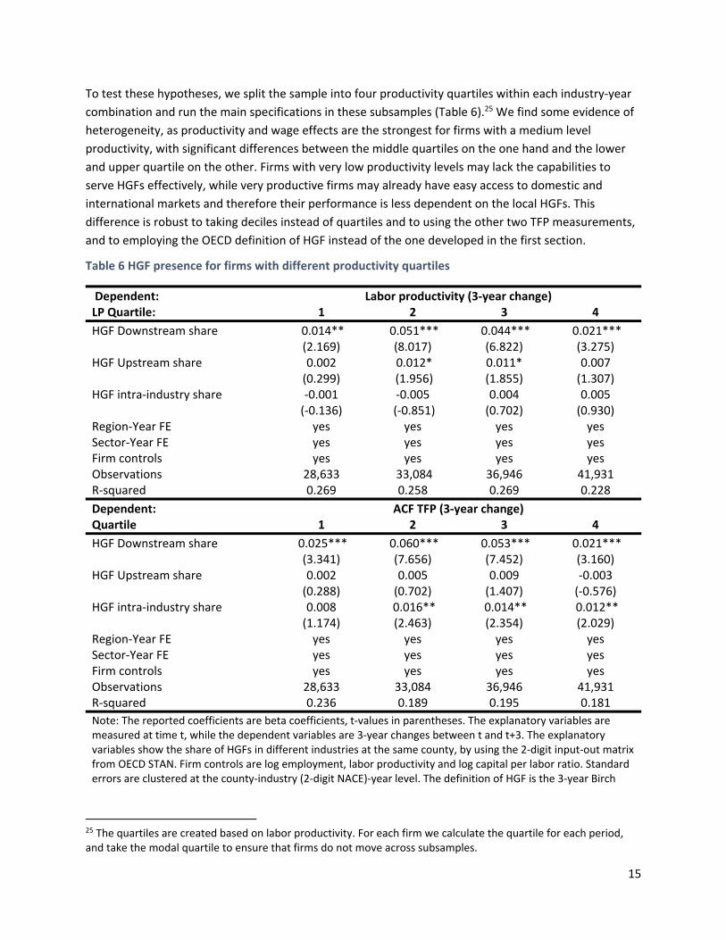
To test these hypotheses, we split the sample into four productivity quartiles within each industry‐year

combination and run the main specifications in these subsamples (Table 6).25 We find some evidence of

heterogeneity, as productivity and wage effects are the strongest for firms with a medium level

productivity, with significant differences between the middle quartiles on the one hand and the lower

and upper quartile on the other. Firms with very low productivity levels may lack the capabilities to

serve HGFs effectively, while very productive firms may already have easy access to domestic and

international markets and therefore their performance is less dependent on the local HGFs. This

difference is robust to taking deciles instead of quartiles and to using the other two TFP measurements,

and to employing the OECD definition of HGF instead of the one developed in the first section.

Table 6 HGF presence for firms with different productivity quartiles

Dependent: Labor productivity (3‐year change) LP Quartile: 1 2 3 4

HGF Downstream share 0.014** 0.051*** 0.044*** 0.021*** (2.169) (8.017) (6.822) (3.275)

HGF Upstream share 0.002 0.012* 0.011* 0.007 (0.299) (1.956) (1.855) (1.307)

HGF intra‐industry share ‐0.001 ‐0.005 0.004 0.005 (‐0.136) (‐0.851) (0.702) (0.930)


Dependent: ACF TFP (3‐year change) Quartile 1 2 3 4


HGF Upstream share 0.002 0.005 0.009 ‐0.003 (0.288) (0.702) (1.407) (‐0.576)

HGF intra‐industry share 0.008 0.016** 0.014** 0.012** (1.174) (2.463) (2.354) (2.029)


Note: The reported coefficients are beta coefficients, t‐values in parentheses. The explanatory variables are measured at time t, while the dependent variables are 3‐year changes between t and t+3. The explanatory variables show the share of HGFs in different industries at the same county, by using the 2‐digit input‐out matrix from OECD STAN. Firm controls are log employment, labor productivity and log capital per labor ratio. Standard errors are clustered at the county‐industry (2‐digit NACE)‐year level. The definition of HGF is the 3‐year Birch

25 The quartiles are created based on labor productivity. For each firm we calculate the quartile for each period, and take the modal quartile to ensure that firms do not move across subsamples.

16

employment definition. We split the sample to productivity quartile within industry‐year and take the model quartile for each firm.

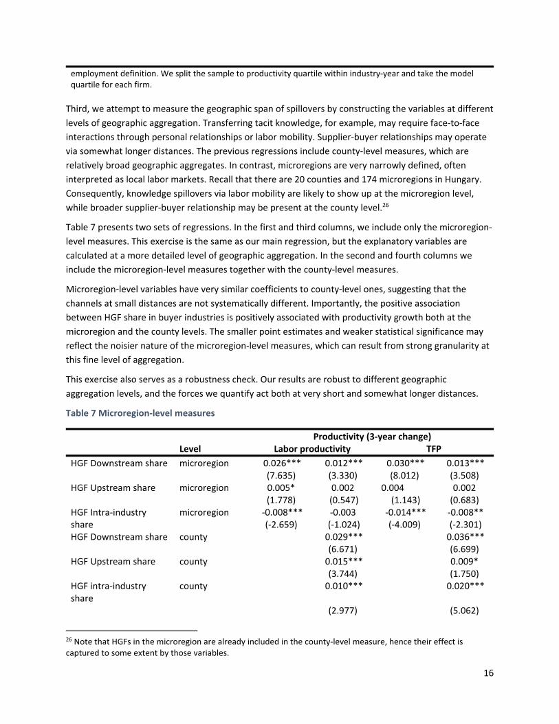
Third, we attempt to measure the geographic span of spillovers by constructing the variables at different

levels of geographic aggregation. Transferring tacit knowledge, for example, may require face‐to‐face

interactions through personal relationships or labor mobility. Supplier‐buyer relationships may operate

via somewhat longer distances. The previous regressions include county‐level measures, which are

relatively broad geographic aggregates. In contrast, microregions are very narrowly defined, often

interpreted as local labor markets. Recall that there are 20 counties and 174 microregions in Hungary.

Consequently, knowledge spillovers via labor mobility are likely to show up at the microregion level,

while broader supplier‐buyer relationship may be present at the county level.26

Table 7 presents two sets of regressions. In the first and third columns, we include only the microregion‐

level measures. This exercise is the same as our main regression, but the explanatory variables are

calculated at a more detailed level of geographic aggregation. In the second and fourth columns we

include the microregion‐level measures together with the county‐level measures.

Microregion‐level variables have very similar coefficients to county‐level ones, suggesting that the

channels at small distances are not systematically different. Importantly, the positive association

between HGF share in buyer industries is positively associated with productivity growth both at the

microregion and the county levels. The smaller point estimates and weaker statistical significance may

reflect the noisier nature of the microregion‐level measures, which can result from strong granularity at

this fine level of aggregation.

This exercise also serves as a robustness check. Our results are robust to different geographic

aggregation levels, and the forces we quantify act both at very short and somewhat longer distances.

Table 7 Microregion‐level measures

Productivity (3‐year change) Level Labor productivity TFP

HGF Downstream share microregion 0.026*** 0.012*** 0.030*** 0.013*** (7.635) (3.330) (8.012) (3.508)

HGF Upstream share microregion 0.005* 0.002 0.004 0.002 (1.778) (0.547) (1.143) (0.683)

HGF Intra‐industry share

microregion ‐0.008*** ‐0.003 ‐0.014*** ‐0.008** (‐2.659) (‐1.024) (‐4.009) (‐2.301)

HGF Downstream share county

0.029***

0.036*** (6.671)

(6.699)

HGF Upstream share county

0.015***

0.009* (3.744)

(1.750)

HGF intra‐industry share

county

0.010***

0.020***

(2.977)

(5.062)

26 Note that HGFs in the microregion are already included in the county‐level measure, hence their effect is captured to some extent by those variables.

17

Region‐Year FE

yes yes yes yes Sector‐Year FE

yes yes yes yes

Firm controls

yes yes yes yes Observations

140,594 140,594 140,594 140,594

R‐squared 0.215 0.216 0.169 0.170

Note: The reported coefficients are beta coefficients, t‐values in parentheses. The explanatory variables are measured at time t, while the dependent variables are 3‐year changes between t and t+3. The explanatory variables show the share of HGFs in different industries at the same microregion and county, by using the 2‐digit input‐out matrix from OECD STAN. Firm controls are log employment, labor productivity and log capital per labor ratio. Standard errors are clustered at the county‐industry (2‐digit NACE)‐year level. The definition of HGF is the 3‐year Birch employment definition.

3.3 Robustness checks

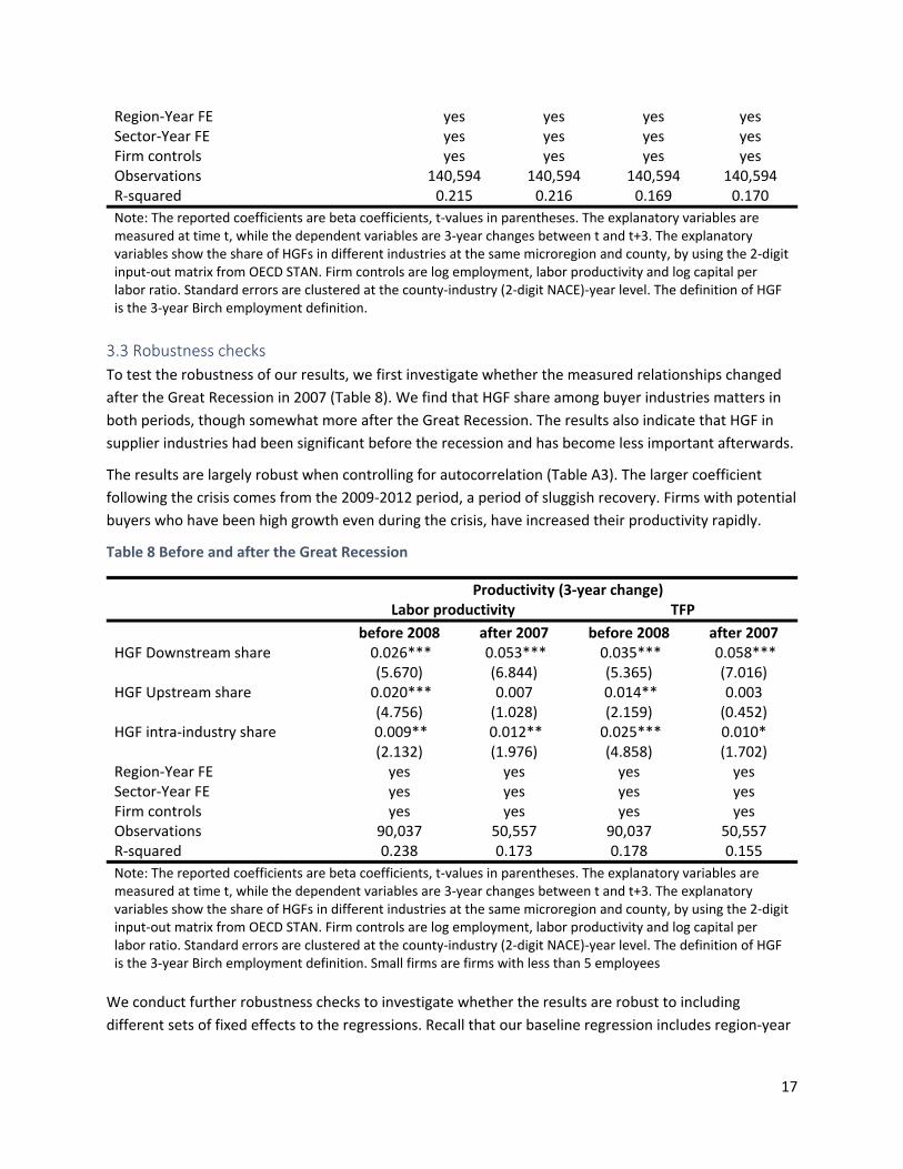
To test the robustness of our results, we first investigate whether the measured relationships changed

after the Great Recession in 2007 (Table 8). We find that HGF share among buyer industries matters in

both periods, though somewhat more after the Great Recession. The results also indicate that HGF in

supplier industries had been significant before the recession and has become less important afterwards.

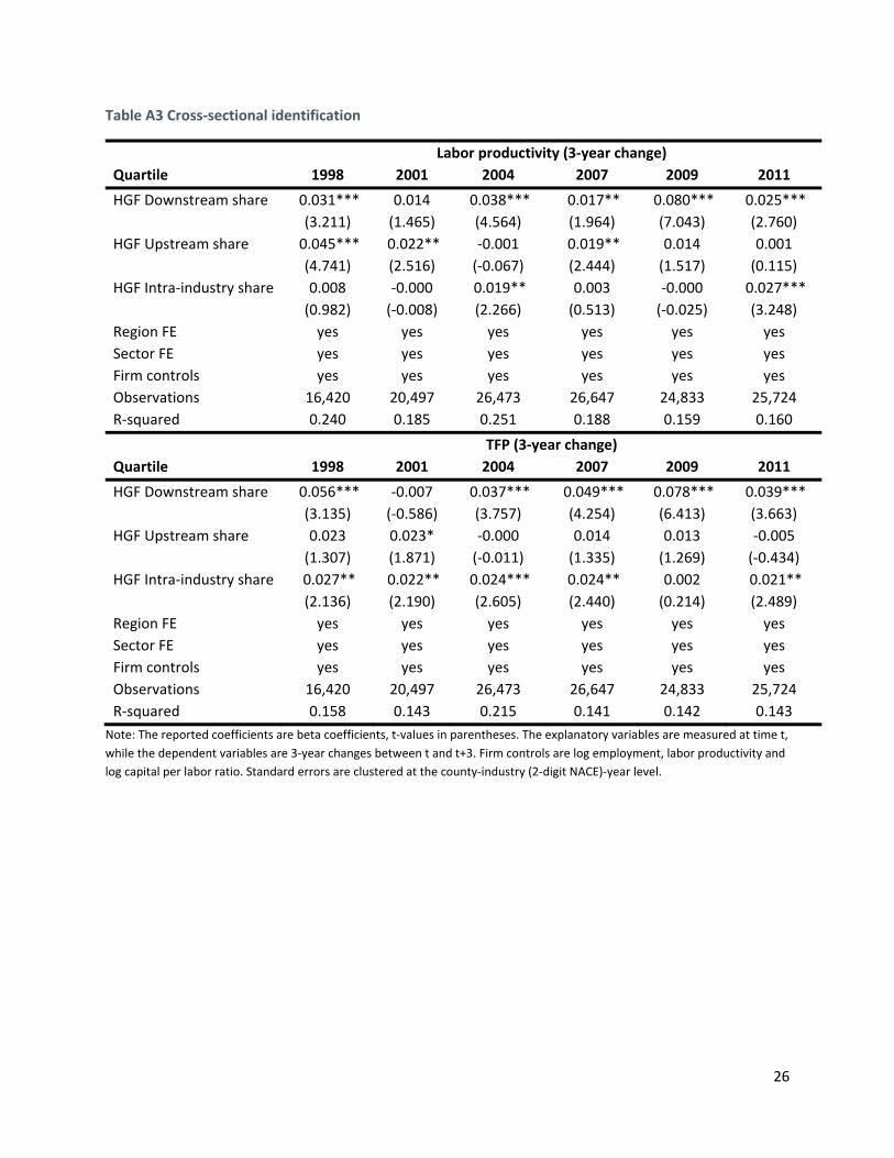
The results are largely robust when controlling for autocorrelation (Table A3). The larger coefficient

following the crisis comes from the 2009‐2012 period, a period of sluggish recovery. Firms with potential

buyers who have been high growth even during the crisis, have increased their productivity rapidly.

Table 8 Before and after the Great Recession

Productivity (3‐year change) Labor productivity TFP

before 2008 after 2007 before 2008 after 2007 HGF Downstream share 0.026*** 0.053*** 0.035*** 0.058***

(5.670) (6.844) (5.365) (7.016) HGF Upstream share 0.020*** 0.007 0.014** 0.003

(4.756) (1.028) (2.159) (0.452) HGF intra‐industry share 0.009** 0.012** 0.025*** 0.010*

(2.132) (1.976) (4.858) (1.702) Region‐Year FE yes yes yes yes Sector‐Year FE yes yes yes yes Firm controls yes yes yes yes Observations 90,037 50,557 90,037 50,557 R‐squared 0.238 0.173 0.178 0.155

Note: The reported coefficients are beta coefficients, t‐values in parentheses. The explanatory variables are measured at time t, while the dependent variables are 3‐year changes between t and t+3. The explanatory variables show the share of HGFs in different industries at the same microregion and county, by using the 2‐digit input‐out matrix from OECD STAN. Firm controls are log employment, labor productivity and log capital per labor ratio. Standard errors are clustered at the county‐industry (2‐digit NACE)‐year level. The definition of HGF is the 3‐year Birch employment definition. Small firms are firms with less than 5 employees

We conduct further robustness checks to investigate whether the results are robust to including

different sets of fixed effects to the regressions. Recall that our baseline regression includes region‐year

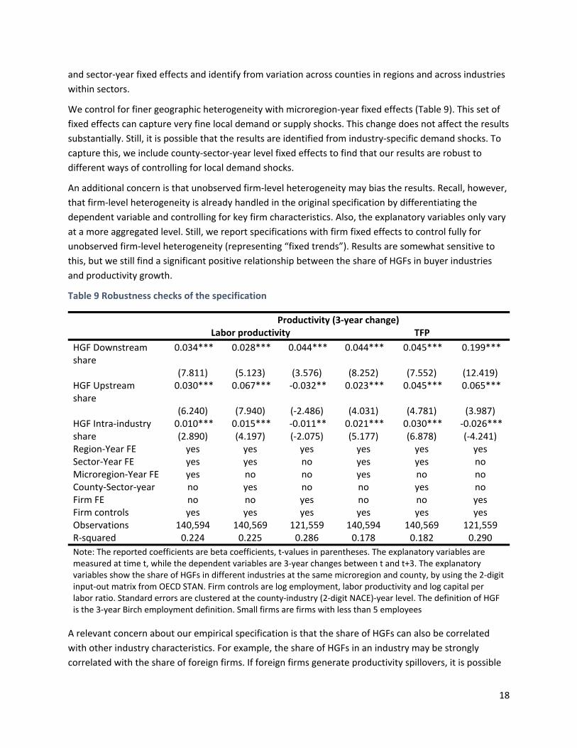
18

and sector‐year fixed effects and identify from variation across counties in regions and across industries

within sectors.

We control for finer geographic heterogeneity with microregion‐year fixed effects (Table 9). This set of

fixed effects can capture very fine local demand or supply shocks. This change does not affect the results

substantially. Still, it is possible that the results are identified from industry‐specific demand shocks. To

capture this, we include county‐sector‐year level fixed effects to find that our results are robust to

different ways of controlling for local demand shocks.

An additional concern is that unobserved firm‐level heterogeneity may bias the results. Recall, however,

that firm‐level heterogeneity is already handled in the original specification by differentiating the

dependent variable and controlling for key firm characteristics. Also, the explanatory variables only vary

at a more aggregated level. Still, we report specifications with firm fixed effects to control fully for

unobserved firm‐level heterogeneity (representing “fixed trends”). Results are somewhat sensitive to

this, but we still find a significant positive relationship between the share of HGFs in buyer industries

and productivity growth.

Table 9 Robustness checks of the specification

Productivity (3‐year change) Labor productivity TFP

HGF Downstream share

0.034*** 0.028*** 0.044*** 0.044*** 0.045*** 0.199***

(7.811) (5.123) (3.576) (8.252) (7.552) (12.419)

HGF Upstream share

0.030*** 0.067*** ‐0.032** 0.023*** 0.045*** 0.065***

(6.240) (7.940) (‐2.486) (4.031) (4.781) (3.987)


0.010*** 0.015*** ‐0.011** 0.021*** 0.030*** ‐0.026*** (2.890) (4.197) (‐2.075) (5.177) (6.878) (‐4.241)

Region‐Year FE yes yes yes yes yes yes Sector‐Year FE yes yes no yes yes no Microregion‐Year FE yes no no yes no no County‐Sector‐year no yes no no yes no Firm FE no no yes no no yes Firm controls yes yes yes yes yes yes Observations 140,594 140,569 121,559 140,594 140,569 121,559 R‐squared 0.224 0.225 0.286 0.178 0.182 0.290

Note: The reported coefficients are beta coefficients, t‐values in parentheses. The explanatory variables are measured at time t, while the dependent variables are 3‐year changes between t and t+3. The explanatory variables show the share of HGFs in different industries at the same microregion and county, by using the 2‐digit input‐out matrix from OECD STAN. Firm controls are log employment, labor productivity and log capital per labor ratio. Standard errors are clustered at the county‐industry (2‐digit NACE)‐year level. The definition of HGF is the 3‐year Birch employment definition. Small firms are firms with less than 5 employees

A relevant concern about our empirical specification is that the share of HGFs can also be correlated

with other industry characteristics. For example, the share of HGFs in an industry may be strongly

correlated with the share of foreign firms. If foreign firms generate productivity spillovers, it is possible

19

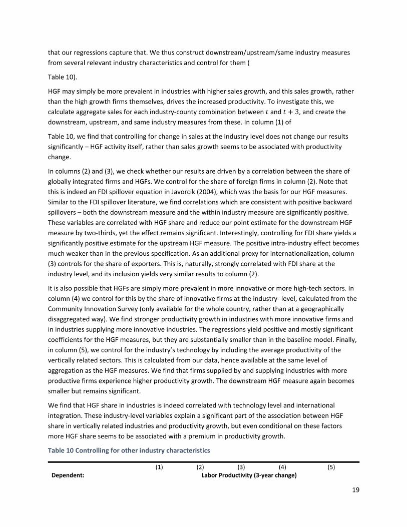
that our regressions capture that. We thus construct downstream/upstream/same industry measures

from several relevant industry characteristics and control for them (

Table 10).

HGF may simply be more prevalent in industries with higher sales growth, and this sales growth, rather

than the high growth firms themselves, drives the increased productivity. To investigate this, we

calculate aggregate sales for each industry‐county combination between 𝑡 and 𝑡 3, and create the downstream, upstream, and same industry measures from these. In column (1) of

Table 10, we find that controlling for change in sales at the industry level does not change our results

significantly – HGF activity itself, rather than sales growth seems to be associated with productivity

change.

In columns (2) and (3), we check whether our results are driven by a correlation between the share of

globally integrated firms and HGFs. We control for the share of foreign firms in column (2). Note that

this is indeed an FDI spillover equation in Javorcik (2004), which was the basis for our HGF measures.

Similar to the FDI spillover literature, we find correlations which are consistent with positive backward

spillovers – both the downstream measure and the within industry measure are significantly positive.

These variables are correlated with HGF share and reduce our point estimate for the downstream HGF

measure by two‐thirds, yet the effect remains significant. Interestingly, controlling for FDI share yields a

significantly positive estimate for the upstream HGF measure. The positive intra‐industry effect becomes

much weaker than in the previous specification. As an additional proxy for internationalization, column

(3) controls for the share of exporters. This is, naturally, strongly correlated with FDI share at the

industry level, and its inclusion yields very similar results to column (2).

It is also possible that HGFs are simply more prevalent in more innovative or more high‐tech sectors. In

column (4) we control for this by the share of innovative firms at the industry‐ level, calculated from the

Community Innovation Survey (only available for the whole country, rather than at a geographically

disaggregated way). We find stronger productivity growth in industries with more innovative firms and

in industries supplying more innovative industries. The regressions yield positive and mostly significant

coefficients for the HGF measures, but they are substantially smaller than in the baseline model. Finally,

in column (5), we control for the industry’s technology by including the average productivity of the

vertically related sectors. This is calculated from our data, hence available at the same level of

aggregation as the HGF measures. We find that firms supplied by and supplying industries with more

productive firms experience higher productivity growth. The downstream HGF measure again becomes

smaller but remains significant.

We find that HGF share in industries is indeed correlated with technology level and international

integration. These industry‐level variables explain a significant part of the association between HGF

share in vertically related industries and productivity growth, but even conditional on these factors

more HGF share seems to be associated with a premium in productivity growth.

Table 10 Controlling for other industry characteristics

(1) (2) (3) (4) (5) Dependent: Labor Productivity (3‐year change)

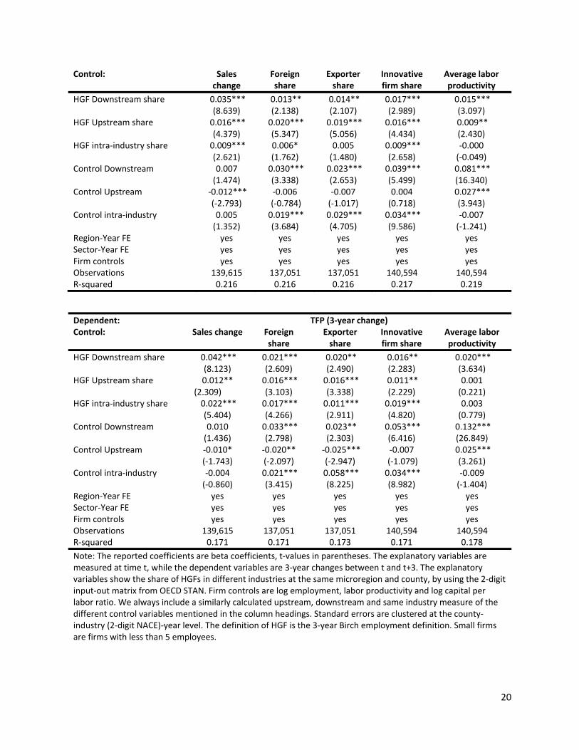
20

Control: Sales change

Foreign share

Exporter share

Innovative firm share

Average labor productivity

HGF Downstream share 0.035*** 0.013** 0.014** 0.017*** 0.015*** (8.639) (2.138) (2.107) (2.989) (3.097)

HGF Upstream share 0.016*** 0.020*** 0.019*** 0.016*** 0.009** (4.379) (5.347) (5.056) (4.434) (2.430)

HGF intra‐industry share 0.009*** 0.006* 0.005 0.009*** ‐0.000 (2.621) (1.762) (1.480) (2.658) (‐0.049)

Control Downstream 0.007 0.030*** 0.023*** 0.039*** 0.081*** (1.474) (3.338) (2.653) (5.499) (16.340)

Control Upstream ‐0.012*** ‐0.006 ‐0.007 0.004 0.027*** (‐2.793) (‐0.784) (‐1.017) (0.718) (3.943)

Control intra‐industry 0.005 0.019*** 0.029*** 0.034*** ‐0.007 (1.352) (3.684) (4.705) (9.586) (‐1.241)

Region‐Year FE yes yes yes yes yes Sector‐Year FE yes yes yes yes yes Firm controls yes yes yes yes yes Observations 139,615 137,051 137,051 140,594 140,594 R‐squared 0.216 0.216 0.216 0.217 0.219

Dependent: TFP (3‐year change) Control: Sales change Foreign

share Exporter share

Innovative firm share

Average labor productivity

HGF Downstream share 0.042*** 0.021*** 0.020** 0.016** 0.020*** (8.123) (2.609) (2.490) (2.283) (3.634)

HGF Upstream share 0.012** 0.016*** 0.016*** 0.011** 0.001 (2.309) (3.103) (3.338) (2.229) (0.221)

HGF intra‐industry share 0.022*** 0.017*** 0.011*** 0.019*** 0.003 (5.404) (4.266) (2.911) (4.820) (0.779)

Control Downstream 0.010 0.033*** 0.023** 0.053*** 0.132*** (1.436) (2.798) (2.303) (6.416) (26.849)

Control Upstream ‐0.010* ‐0.020** ‐0.025*** ‐0.007 0.025*** (‐1.743) (‐2.097) (‐2.947) (‐1.079) (3.261)

Control intra‐industry ‐0.004 0.021*** 0.058*** 0.034*** ‐0.009 (‐0.860) (3.415) (8.225) (8.982) (‐1.404)

Region‐Year FE yes yes yes yes yes Sector‐Year FE yes yes yes yes yes Firm controls yes yes yes yes yes Observations 139,615 137,051 137,051 140,594 140,594 R‐squared 0.171 0.171 0.173 0.171 0.178

Note: The reported coefficients are beta coefficients, t‐values in parentheses. The explanatory variables are measured at time t, while the dependent variables are 3‐year changes between t and t+3. The explanatory variables show the share of HGFs in different industries at the same microregion and county, by using the 2‐digit input‐out matrix from OECD STAN. Firm controls are log employment, labor productivity and log capital per labor ratio. We always include a similarly calculated upstream, downstream and same industry measure of the different control variables mentioned in the column headings. Standard errors are clustered at the county‐industry (2‐digit NACE)‐year level. The definition of HGF is the 3‐year Birch employment definition. Small firms are firms with less than 5 employees.

21

4 Conclusions

High‐growth firms have a disproportionate ability to create jobs and generate output. But there is less

evidence and understanding about whether the benefits to economic growth outweigh the costs they

impose on other firms. To understand the impact of HGFs on the economy as a whole, we rely on

detailed administrative microdata from Hungary. We find that productivity growth of firms in Hungary is

stronger if they serve industries with more HGFs. The fact that the premium in productivity growth is

associated with growth in sales and that spillovers exceed local labor markets suggests that the surge in

demand generated by HGFs may allow their suppliers to exploit economies of scale. Not only do HGFs

have positive spillovers, but they benefit more firms in the middle of the productivity distribution. Firms

in the bottom quartile of the distribution are not productive enough to take fuller advantage of HGFs

demand. Firms in the top quartile of the distribution have access to wider markets and do not depend

on HGFs as much. We also find that manufacturing firms are better able to benefit from the presence of

HGFs than services firms. Lastly, we ascertain that the spillover effects are still present at a finer

geographical level.

The results are robust to alternative definitions of HGFs, sample and estimation method. As discussed in

the paper, establishing causality presents significant econometric challenges. The fact that they continue

to hold when controlling for a plethora of factors and are not sensitive to several robustness checks

gives us confidence in them.

The paper provides evidence for policy makers who may be concerned about directing scarce resources

towards supporting HGFs, instead of using these resources for firms in other parts of the economy. It

also highlights that the attention and resources given to HGFs can benefit other firms in the economy.

References

Ackerberg, D. A., Caves, K., & Frazer, G. (2015). Identification properties of recent production function

estimators. Econometrica, 83(6), 2411‐2451.

Ács, Z. 2010. “High‐Impact Entrepreneurship”. Chapter 7 in Z.J. Acs, D.B. Audretsch (eds.), Handbook of

Entrepreneurship Research, 165. International Handbook Series on Entrepreneurship 5

Angrist, J. D. (2014). The perils of peer effects. Labor Economics, 30, 98‐108.

Audretsch, D. B. 2005. “The Knowledge Spillover Theory of Entrepreneurship and Economic Growth”.

The Emergence of Entrepreneurial Economics: Research on Technological Innovation, Management and

Policy, Vol. 9: 37‐54.

Autio, E., Kronlund, M., and Kovalainen, A. 2007. “High‐Growth SME Support Initiatives in Nine

Countries: Analysis, Categorization, and Recommendations”. Report Prepared for the Finnish Ministry of

Trade and Industry. Publications, Industries Department.

Birch, D. L. (1981). Who creates jobs? The public interest, (65), 3.

Blalock, G., & Gertler, P. J. (2008). Welfare gains from foreign direct investment through technology

transfer to local suppliers. Journal of International Economics, 74(2), 402‐421.

22

Briant, A., Combes, P.P. and Lafourcade, M. (2010) “Dots to boxes: Do the size and shape of spatial units

jeopardize economic geography estimations?” Journal of Urban Economics, 67(3), pp.287‐302.

Carree, M. A., and A. Roy Thurik A. R. (2010): The impact of entrepreneurship on economic growth,

in Handbook of entrepreneurship research (pp. 557‐594). Springer, New York, NY.

Coad, A., Daunfeldt, S. O., Hölzl, W., Johansson, D., & Nightingale, P. (2014). High‐growth firms:

introduction to the special section. Industrial and Corporate Change, 23(1), 91‐112.

Foster, L. S., Grim, C. A., Haltiwanger, J., & Wolf, Z. (2017). Macro and Micro Dynamics of Productivity:

From Devilish Details to Insights (No. w23666). National Bureau of Economic Research.

Girma, S., Gong, Y., Görg, H., & Lancheros, S. (2015). Estimating direct and indirect effects of foreign

direct investment on firm productivity in the presence of interactions between firms. Journal of

International Economics, 95(1), 157‐169.

Görg, H., & Greenaway, D. (2004). Much ado about nothing? Do domestic firms really benefit from

foreign direct investment? The World Bank Research Observer, 19(2), 171‐197.

Haltiwanger, J., Jarmin, R. S., & Miranda, J. (2013). Who creates jobs? Small versus large versus young.

Review of Economics and Statistics, 95(2), 347‐361.

Harrison, A., & Rodríguez‐Clare, A. (2010). Trade, foreign investment, and industrial policy for

developing countries. In Handbook of development economics (Vol. 5, pp. 4039‐4214). Elsevier.

Hausmann, R., & Rodrik, D. (2003). Economic development as self‐discovery. Journal of development

Economics, 72(2), 603‐633.

Hillberry, R. and Hummels, D. (2008). Trade responses to geographic frictions: A decomposition using

micro‐data. European Economic Review, 52(3), pp.527‐550.

Hsieh, C. T., & Klenow, P. J. (2009). Misallocation and manufacturing TFP in China and India. The

Quarterly journal of economics, 124(4), 1403‐1448.

Javorcik, B. S. (2004). Does foreign direct investment increase the productivity of domestic firms? In

search of spillovers through backward linkages. The American Economic Review, 94(3), 605‐627.

OECD (2010), High‐Growth Enterprises: What Governments Can Do to Make a Difference, OECD

Publishing, Paris. DOI: http://dx.doi.org/10.1787/9789264048782‐en.

OECD (2016), "High‐growth enterprises rate", in Entrepreneurship at a Glance 2016, OECD Publishing,

Paris, http://dx.doi.org/10.1787/entrepreneur_aag‐2016‐23‐en.

Rodrik, D. (2005). Growth strategies. Handbook of economic growth, 1, 967‐1014.

Rosenthal, Stuart and William Strange (2004). “Evidence of the Nature and Sources of Agglomeration

Economies.” Handbook of Regional and Urban Economics Vol. 4. Pp. 2119‐2171.

Semjén, András és Tóth, István János és Fazekas, Mihály (2009) Az egyszerűsített vállalkozói adó (eva)

tapasztalatai vállalkozói interjúk alapján. In: Rejtett gazdaság. KTI Könyvek (11). MTA

Közgazdaságtudományi Intézet (KTI), Budapest, pp. 131‐149. ISBN 978‐963‐9796‐58‐4

23

Tonin, M. (2011). Minimum wage and tax evasion: Theory and evidence. Journal of Public Economics,

95(11‐12), 1635‐1651.

World Bank (2018), High Growth Firms: Facts and Fiction of High Growth Entrepreneurship in Developing

Countries. Forthcoming.

24

Appendix: Further tables

Table A1 Main results with other productivity estimators

Dependent: Productivity (3‐year growth)

TFP (FE) TFP (Wooldridge)

HGF Downstream share 0.040*** 0.039*** 0.044*** 0.043***

(9.704) (9.467) (10.628) (10.423)

HGF Upstream share 0.015*** 0.014*** 0.012*** 0.012***

(3.643) (3.598) (3.087) (3.048)


0.010***

0.010***

(2.846)

(2.921)

Region‐Year FE yes yes yes yes

Sector‐Year FE yes yes yes yes

Firm controls yes yes yes yes

Observations 140,594 140,594 140,594 140,594

R‐squared 0.208 0.208 0.187 0.187

Note: The reported coefficients are beta coefficients, t‐values in parentheses. The explanatory variables are measured at time t,

while the dependent variables are 3‐year changes between t and t+3. Firm controls are log employment, labor productivity and

log capital per labor ratio. Standard errors are clustered at the county‐industry (2‐digit NACE)‐year level. The definition of HGF

is the 3‐year Birch employment definition.

25

Table A2 Main results with OECD employment HGF definition

Dependent: Productivity (3‐year growth)

Labor productivity TFP


HGF Upstream share ‐0.006 ‐0.007 ‐0.011* ‐0.012* (‐1.359) (‐1.450) (‐1.755) (‐1.902)


0.014***

0.025*** (4.509)

(7.005)





Dependent: Size (3‐year growth)

Employment (ln) Sales (ln)

HGF Downstream share ‐0.000 ‐0.000 0.025*** 0.025*** (‐0.070) (‐0.068) (4.759) (4.790)

HGF Upstream share 0.002 0.002 ‐0.003 ‐0.003 (0.538) (0.487) (‐0.576) (‐0.611)


0.009***

0.007* (2.843)

(1.926)





Dependent: Income (3‐year growth)

Average wage (ln) ROA


HGF Upstream share 0.004 0.004 ‐0.006 ‐0.006 (0.627) (0.682) (‐1.187) (‐1.308)


‐0.011***

0.019*** (‐3.135)

(5.758)







log capital per labor ratio. Standard errors are clustered at the county‐industry (2‐digit NACE)‐year level. The definition of HGF

is the 3‐year OECD employment definition.

26

Table A3 Cross‐sectional identification

Labor productivity (3‐year change)

Quartile 1998 2001 2004 2007 2009 2011

HGF Downstream share 0.031*** 0.014 0.038*** 0.017** 0.080*** 0.025*** (3.211) (1.465) (4.564) (1.964) (7.043) (2.760)

HGF Upstream share 0.045*** 0.022** ‐0.001 0.019** 0.014 0.001 (4.741) (2.516) (‐0.067) (2.444) (1.517) (0.115)

HGF Intra‐industry share 0.008 ‐0.000 0.019** 0.003 ‐0.000 0.027*** (0.982) (‐0.008) (2.266) (0.513) (‐0.025) (3.248)

Region FE yes yes yes yes yes yes

Sector FE yes yes yes yes yes yes

Firm controls yes yes yes yes yes yes

Observations 16,420 20,497 26,473 26,647 24,833 25,724

R‐squared 0.240 0.185 0.251 0.188 0.159 0.160

TFP (3‐year change)

Quartile 1998 2001 2004 2007 2009 2011

HGF Downstream share 0.056*** ‐0.007 0.037*** 0.049*** 0.078*** 0.039*** (3.135) (‐0.586) (3.757) (4.254) (6.413) (3.663)

HGF Upstream share 0.023 0.023* ‐0.000 0.014 0.013 ‐0.005 (1.307) (1.871) (‐0.011) (1.335) (1.269) (‐0.434)

HGF Intra‐industry share 0.027** 0.022** 0.024*** 0.024** 0.002 0.021** (2.136) (2.190) (2.605) (2.440) (0.214) (2.489)

Region FE yes yes yes yes yes yes

Sector FE yes yes yes yes yes yes

Firm controls yes yes yes yes yes yes

Observations 16,420 20,497 26,473 26,647 24,833 25,724

R‐squared 0.158 0.143 0.215 0.141 0.142 0.143



log capital per labor ratio. Standard errors are clustered at the county‐industry (2‐digit NACE)‐year level.

High-Growth Firms: Rising Tide Lifts All Boats

Documents

Transcript of High-Growth Firms: Rising Tide Lifts All Boats