High frequency trading (Machine learning, Neural networks),

Algorithmic trading

Machine learning for high frequency trading and market microstructure

data and problems.

Machine learning is a vibrant subfield of computer science that draws on

models and methods from statistics, algorithms, computational

complexity, artificial intelligence, control theory, and a variety of other

disciplines. Its primary focus is on computationally and informationally

efficient algorithms for inferring good predictive models from large data

sets.

The special challenges for machine learning presented by HFT generally

arise from the very fine granularity of the data — often microstructure

data at the resolution of individual orders, (partial) executions, hidden

liquidity, and cancellations —

• understanding of how such low-level data relates to actionable

circumstances (such as profitably buying or selling shares, optimally

executing a large order, etc,

• how the distribution of liquidity in the order book relates to future price

movements,

• feature selection or feature engineering

- are the important process in machine learning for HFT

High Frequency Data for Machine Learning

High frequency trading - holding periods, order types (e.g. passive versus

aggressive), and strategies (momentum or reversion, directional or

liquidity provision, etc.).

Data driving HFT activity tends to be the most granular available.

Typically microstructure data - every order placed, every execution, and

every cancellation, and reconstruction (at least for equities) of the full

limit order book.

A single day’s worth of microstructure data on a highly liquid stock is

measured in gigabytes. Storing this data historically for any meaningful

period and number of names requires both compression and significant

disk usage; processing this data efficiently generally requires streaming

through the data by only uncompressing small amounts at a time.

What systematic signal or information is contained in microstructure

data? - What “features” or variables can we extract from this extremely

granular, lower-level data.

Limit Order Trading and Market Simulation

Limit order markets: By this we mean that buyers and sellers specify

not only their desired volumes, but their desired prices as well. A limit

order to buy (respectively, sell) V shares at price p may partially or

completely execute at prices at or below p (at or above p).

For example, suppose that NVIDIA Corp. (NVDA) is currently trading at

roughly $27.22 a share (see Figure 1, which shows an actual snapshot of

an NVDA order book), but we are only willing to buy 1000 shares at

$27.13 a share or lower. We can choose to submit a limit order with this

specification, and our order will be placed in the buy order book, which is

ordered by price, with the highest price at the top (this price is referred to

as the bid; the lowest sell price is called the ask). In the example

provided, our order would be placed immediately after the extant order

for 109 shares at $27.13; though we offer the same price, this order has

arrived before ours. If an arriving limit order can be immediately

executed with orders on the opposing book, the executions occur. For

example, a limit order to buy 2500 shares at $27.27will cause execution

with the limit sell orders for 713 shares at $27.22, and the 1000-share and

640-share sell orders at $27.27, for a total of 2353 shares executed. The

remaining (unexecuted) 147 shares of the arriving buy order will become

the new bid at $27.27. It is important to note that the prices of executions

are the prices specified in the limit orders already in the books, not the

prices of the incoming order that is immediately executed. Thus we

receive successively worse prices as we consume orders deeper in the

opposing book.

Performance and policies found by RL vary with stock properties such as

liquidity, volume traded, and volatility

Submit and leave (S&L) policies

State-based strategies – strategies that can examine salient features of the

current order books and our own activity – in order to decide what to do

next.

Variables: elapsed time t, remaining inventory i, which represent how

much time of the horizon H has passed and how many shares we have

left to execute in the target volume V. Different resolutions of accuracy

will be investigated for these variables, which we refer to as private

variables, since they are essentially only known and of primary concern

to our execution strategy. More precisely, we pick I and T, which are the

resolutions (maximum values) of the private variables i and t,

respectively. I represents the number of inventory units our policy can

distinguish between – if V = 10,000 shares, and I = 4, our remaining

inventory is represented in rounded units of V/I= 2,500 shares each.

Similarly, we divide the time horizon H into T distinct points at which

the policy is allowed to observe the state and take an action; for H= 2 min

and T= 4 we can submit a revised limit order every 30 seconds, and the

time remaining variable t can assume values from 0 (start of the episode)

down to 4 (last decision point of the episode).

Additional state variables: market variables, a state has the form

xm = <t, i, o1, …, oR>, where the oj are market variables.

Action space: simple limit order price at which to reposition all of our

remaining inventory, for the problem of selling V shares, action a

corresponds to placing a limit order for all of our unexecuted shares at

price ask - a. Thus we are effectively withdrawing any previous

outstanding limit order we may have (which is indeed supported by the

actual exchanges), and replacing with a new limit order. Thus a may be

positive or negative, with a = 0 corresponding to coming in at the current

ask, positive a corresponding to "crossing the spread" towards the buyers,

and negative a corresponding to placing our order in the sell book.

Rewards: An action from a given state may produce immediate rewards,

which are essentially the proceeds (cash inflows or outflows, depending

on whether we are selling or buying) from any (partial) execution of the

limit order placed. Furthermore, since we view the execution of all V

shares as mandatory, any inventory remaining at the end of time His

immediately executed at market prices --- that is, we eat into the

opposing book to execute, no matter how poor the prices, since we have

run out of time and have no choice.

Measure the execution prices achieved by a policy relative to the mid-

spread price (ask+bid)/2 at the start of the episode in question. Thus, we

are effectively comparing performance to the idealized policy which can

execute all V of its shares immediately at the mid-spread, and thus are

assuming infinite liquidity at that point.

Trading cost of a policy: the underperformance compared to the

midspread baseline.

We assume that commissions and exchange fees are negligible.

Predicting Price Movement from Order Book State

Learn models that themselves profitably decide when to trade and how to

trade:

• The development of features that permit the reliable prediction of

directional price movements from certain states. By “reliable” we do

not mean high accuracy, but just enough that our profitable trades

outweigh our unprofitable ones.

• The development of learning algorithms for execution that capture this

predictability or alpha at sufficiently low trading costs.

First find profitable predictive signals:

• Bid-Ask Spread:

• Price: A feature measuring the recent directional movement of

executed prices.

• Smart Price: A variation on mid-price where the average of the bid and

ask prices is weighted according to their inverse volume.

• Trade Sign: A feature measuring whether buyers or sellers crossed the

spread more frequently in recent executions.

• Bid-Ask Volume Imbalance:

• Signed Transaction Volume:

Features above were normalized. In order to obtain a finite state space,

features were discretized into bins in multiples of standard deviation

units.

Learning algorithm: buying 1 share at the bid-ask midpoint and holding

the position for t seconds, at which point we sell the position, again at the

midpoint; and the opposite action, where we sell at the midpoint and buy

t seconds later. In the first set of experiments we describe, we considered

a short period of t = 10 seconds.

The methodology can now be summarized as follows:

For each of 19 names, order book reconstruction on historical data was

performed.

At each trading opportunity, the current state (the value of the six

microstructure features described above) was computed, and the profit or

loss of both actions (buy then sell, sell then buy) is tabulated via order

book simulation to compute the midpoint movement.

Learning was performed for each name using all of 2008 as the training

data. For each state 𝑥 in the state space, the cumulative payoff for both

actions across all visits to 𝑥 in the training period was computed.

Learning then resulted in a policy π mapping states to action, where 𝜋(𝑥)

is defined to be whichever action yielded the greatest training set

profitability in state 𝑥.

Testing of the learned policy for each each name was performed using

all 2009 data. For each test set visit to state 𝑥, we take the action 𝜋(𝑥)

prescribed by the learned policy, and compute the overall 2009

profitability of this policy.

FIGURE 4: Correlations between feature values and learned policies. For

each of the six features and 19 policies, we project the policy onto just

the single feature compute the correlation between the feature value and

action learned (+1 for buying, -1 for selling). Features indices are in the

order Bid-Ask Spread, Price, Smart Price, Trade Sign, Bid-Ask Volume

Imbalance, Signed Transaction Volume.

FIGURE 5: Comparison of test set profitability across 19 names for

learning with all six features (red bars, identical in each subplot) versus

learning with only a single feature (blue bars).

Optimal strategy found:

• momentum behaviour for time periods of milliseconds to seconds,

• reversion strategies for dozens of seconds to several minutes

Aspects that one must consider when applying machine learning to high

frequency data: the nature of the underlying price formation process, and

the role and limitations of the learning algorithm itself.

Empirical Limitations on High Frequency Trading Profitability

Empirical study estimating the maximum possible profitability of the

most aggressive such practices: trading strategy exclusively employing

market orders and relatively short holding periods.

The overarching fear is that quantitative trading groups, armed with

advanced networking and computing technology and expertise, are in

some way victimizing retail traders and other less sophisticated parties.

The HFT debate often conflates distinct phenomena, confusing, for

instance, dark pools and flash trading, which are essentially new market

mechanisms, with HFT itself, which is a type of trading behaviour

applicable to both existing and emerging exchanges. The core concern

regarding HFT, however, is relatively straightforward: that the ability to

electronically execute trades on extraordinarily short time scales,

combined with the quantitative modelling of massive stores of historical

data, permits a variety of practices unavailable to most parties. A broad

example would be the discovery of very short-term informational

advantages (for instance, by detecting large, slow trades in the market)

and profiting from them by trading rapidly and aggressively.

We demonstrate an upper bound of $21 billion for the entire universe of

U.S. equities in 2008 at the longest holding periods, down to $21 million

or less for the shortest holding periods (see discussion of holding periods

below). Furthermore, we believe these numbers to be vast overestimates

of the profits that could actually be achieved in the real world. These

figures should be contrasted with the approximately $50 trillion annual

trading volume in the same markets. We believe our findings are of

interest in their own right as well as potentially relevant to the ongoing

debate over HFT.

Tension between two basic quantities: the horizon or holding period, as

measured by the length of time for which a (long or short) position in a

stock is held; and the costs of trading, as measured by (at least) the bid-

ask spread that must be crossed by market orders.

We compute the profit or loss of the HF trader in hindsight, and reach

empirical overestimates of profitability.

Data: A small set of the most liquid (and therefore most profitable) stocks

on NASDAQ, and then use a slightly less detailed data set and regression

methods to scale up our estimates to a much larger universe of all US

stocks, and across all exchanges.

Related literature: Aldridge examines foreign exchange trading.

Chaboud et al. study foreign exchange markets: HFT does not cause an

increase in volatility. Hendershott et al. analyze trading of US equities,

and find that HFT improves liquidity. The same authors examine German

markets.

Constraints on HFT: aggressive order placement and short holding

periods. We propose that aggressive orders are the greatest cause for any

concerns about the negative impacts on trading counterparties; passive

order placement can only improve the market both in prices and volumes.

If one of the advantages of (and concerns over) HFT is the ability to very

rapidly take and liquidate positions to profit from short-term

informational advantages, aggressive order placement is necessary.

For these reasons we shall restrict our attention to aggressive order

placement.

We shall consider holding periods as short as 10 milliseconds and as long

as 10 seconds.

Two different sources of raw trading data: order book data and Trade and

Quote, or TAQ, data on a much larger set of stocks and exchanges.

In this framework, we simulate the profitability of the following OT,

whose only parameter is the holding period h:

• At each time t, the OT may either buy or sell v shares, for every integer

v ≥ 0. The purchase or sale of the v shares occurs at market prices; thus

according to the standard U.S. equities limit order mechanism, the OT

crosses the spread and consumes the first v shares on the opposing order

book, receiving possibly progressively worse prices for successive

shares.

• If at time t the OT bought/sold v shares, at time t + h it must liquidate

this position and sell/buy the shares back, again by crossing the spread

and paying market prices on the opposing book. (We later discuss the

effects of allowing a variable holding period.)

• At each time t, the OT makes only that trade (buying or selling, and the

choice of v) that optimizes profitability. Obviously it is this aspect of the

OT that requires knowledge of the future. Note that if no trade at t has

positive profitability, the OT does nothing.

Details:

1. If ℎ   ↓ 0 then v = 0 for most of t. This design for the OT accurately

captures the fundamental tension of (aggressive) HFT. If we denote the

bid-ask spread at time t by st, it is clear that the purchase or sale of even a

single share by the OT will incur transaction costs on the order of at least

½ (st + st+h) — the mean of the spreads at the onset and liquidation of the

position. Larger values for v will increase these costs, since eating further

into the opposing books effectively widens the spreads. Thus, in order for

a trade of v shares to be profitable, the share price must have time to

change enough to cover the spread-based transaction costs. (Since we

omnisciently optimize between buying and selling, as well as the trade

volume, sufficient movement either up or down will result in some

profitable trade.) Of course, the smaller the holding period h, the less

frequently such fluctuations will occur — indeed, we find that for

sufficiently small h, the vast majority of the time the optimal choice is v

= 0 — that is, no trade is made by the OT.

2. Large data ⟹ high computation time.

3. We assume the trades of the OT have no impact on the market.

4. We assume no trading fees or commissions are paid by the HFT.

5. We assume that offers taken by the trader remain on the books,

allowing the trader to repeatedly profit from a single opportunity as often

as 100 times per second.

6. No mixing: We do not allow the OT to enter a postion with a market

order but exit with a limit order (or vice versa).

7. No forward looking strategy

8. We allow trading every 10 milliseconds conditioned on there being any

change.

9. This also replicates the actual HFT during this period.

Omniscient Order Book Trading: Even at the longest holding period of

10 seconds the total 2008 OT profits are only $3.4 billion, down to just

$62,000 for the shortest (10ms) holding period.

Market-Wide Extrapolation

Extrapolate our results to all stocks and all exchanges by utilizing the

broader but somewhat less detailed Trade and Quote (TAQ). We estimate

a primary-to-composite conversion ratio (in a given name, around 50% of

profits come from the primary exchange.

The earlier target 19 stocks traded primarily on NASDAQ, are also traded

on a variety of alternative exchanges that in some instances may offer

better pricing. TAQ data are limited in do not record liquidity offered

beyond the current bid and ask prices.

At each time t, the OT can buy or sell v shares, where v ≥ 0 is an integer

bounded by the number of shares available to buy (sell) at the ask (bid) at

time t as well as the number of shares available to sell (buy) at the bid

(ask) at time t + h. For example, if 100 shares are offered at the ask price

at time t and 50 shares are offered at the bid price at time t + h, then the

OT can only consider buying up to 50 shares at time t. (Since the trader is

omniscient, it can compute these limits even though they depend on

future information.) As before, any position taken at time t must be

liquidated at time t + h.

The modified OT (simulated on TAQ data) occasionally achieves higher

profits than the original OT. Correlation is 0.969. We assume that the

original OT’s profits are closely estimated as a multiple of the modified

OT’s profits. So we directly apply extrapolation ratios.

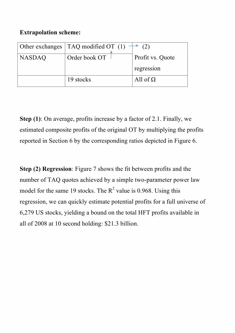
Extrapolation scheme:

Other exchanges TAQ modified OT (1) (2)

Profit vs. Quote

regression

NASDAQ Order book OT

19 stocks All of Ω

Step (1): On average, profits increase by a factor of 2.1. Finally, we

estimated composite profits of the original OT by multiplying the profits

reported in Section 6 by the corresponding ratios depicted in Figure 6.

Step (2) Regression: Figure 7 shows the fit between profits and the

number of TAQ quotes achieved by a simple two-parameter power law

model for the same 19 stocks. The R2 value is 0.968. Using this

regression, we can quickly estimate potential profits for a full universe of

6,279 US stocks, yielding a bound on the total HFT profits available in

all of 2008 at 10 second holding: $21.3 billion.

Machine learning approach offers no easy paths to profitability: Even

if all the features we enumerate here are true predictors of future returns,

and even if all of them line up just right for maximum profit margins, one

still cannot justify trading aggressively and paying the bid-ask spread,

since the magnitude of predictability is not sufficient to cover transaction

costs.

References:

[1] Michael Kearns and Yuriy Nevmyvaka, Machine Learning for Market

Microstructure and High Frequency Trading, in High Frequency Trading

- New Realities for Traders, Markets and Regulators, David Easley,

Marcos Lopez de Prado and Maureen O’Hara editors, Risk Books, 2013.

http://riskbooks.com/book-high-frequency-trading

[2] Yuriy Nevmyvaka, Yi Feng, and Michael Kearns. Reinforcement

Learning for Optimized Trade Execution. In Proceedings of the 23rd

international conference on Machine learning, pages 673–680. ACM,

2006.

[3] A. Kulesza, M. Kearns, and Y. Nevmyvaka. Empirical Limitations on

High Frequency Trading Profitability. Journal of Trading, 5(4):50–62,

2010.

[4] K. Ganchev, M. Kearns, Y. Nevmyvaka, and J. Wortman. Censored

Exploration and the Dark Pool Problem. Communications of the ACM,

53(5):99–107, 2010.

[5] R. Cont and A. Kukanov. Optimal Order Placement in Limit Order

Markets. Technical Report, arXiv.org, 2013.