High Frequency Equities Trading &

Microstructural Cost Effects For

Institutional Orders

Agenda

• HFT – Benefits and Challenges

• Studying the Challenges

– Analyzing an Institutional Order: Separating Impact & Timing Costs

– VWAP Versus Implementation Shortfall Algorithms

– Dark Aggregating Algorithms

• Conclusion

What is High-Frequency Trading?

• Generally fall into two broad categories:

– (1) Electronic Market Making

• Try to profit from the spread between bid and ask prices

• Rarely hold positions over night

• Benefit from „liquidity rebates‟ paid by exchanges and

market centers

– (2) Statistical Arbitrage

• Identify and capitalize on inefficient pricing of

financial instruments

• Market efficiency

• Information/Interest arbitrage

– Inter-venue latency arbitrage

– „Trading ahead‟ of significant order flow

Speed is Everything

• Need ultrafast, high capacity systems to thrive

– Freshest market data on every tradable security

• Nasdaq ITCH or BATS‟ FASTPITCH vs SIP feed (Securities

Information Processor)

• Co-location

– Absolute most minimum time delay, or latency

• EMM‟s send and cancel thousands of orders simultaneously

to effectively manage risk

NYSE Message Traffic

Source: Rosenblatt Securities

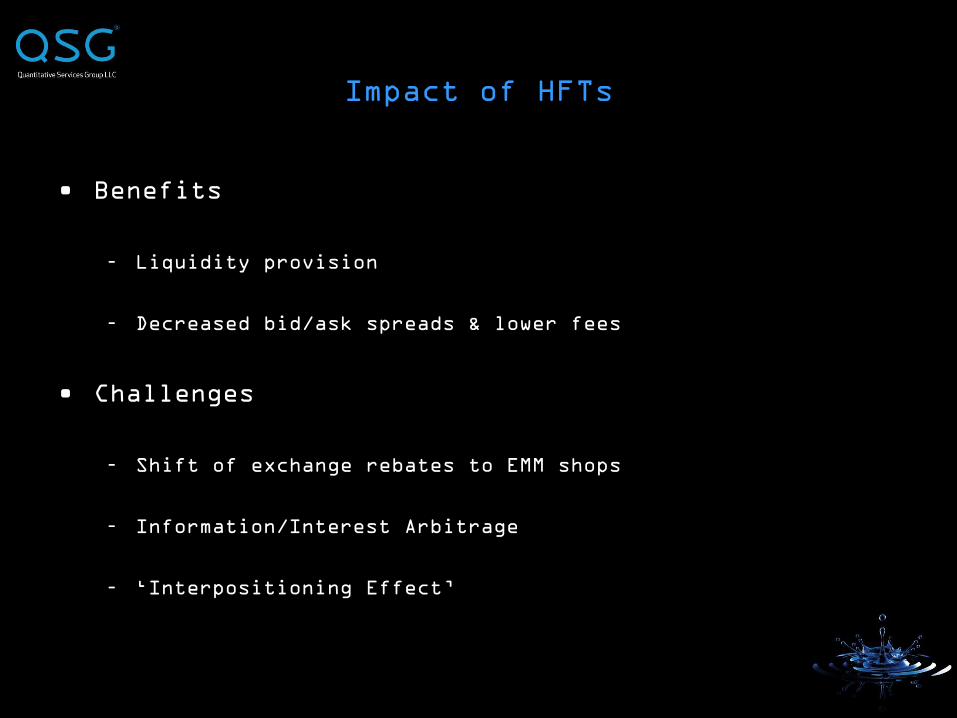
Impact of HFTs

• Benefits

– Liquidity provision

– Decreased bid/ask spreads & lower fees

• Challenges

– Shift of exchange rebates to EMM shops

– Information/Interest Arbitrage

– „Interpositioning Effect‟

• In James Brigagliano‟s testimony before the Senate

Banking Subcommittee on Securities, Insurance &

Investment, October 28 of last year:

– “This quicker access could, for example, enable

high-frequency traders to successfully implement

„momentum‟ strategies designed to prompt sharp price

movements and then profit from the resulting short-

term volatility”

– “In combination with a „liquidity detection‟

strategy that seeks solely to ascertain whether

there is a large buyer or seller in the market (such

as an institutional investor), a high-frequency

trader may be able to profit from trading ahead of

the large order”

Challenges

Inter-venue Latency ArbitrageInterpositioning Effect: Case 1

$30.22

Bid

$30.24

Offer

$30.23

Bid

$30.24

Offer

Broker enters $30.23

Bid on Nasdaq,

decreasing spread

to $0.01

An HFT sees this on his Nasdaq ITCH feed

before others relying on the

consolidated feed and INSTANTANEOUSLY

bids $30.23 on another venue such as

BATS, NYSE Arca or Direct Edge

NasdaqBATS

$30.21

Bid

$30.25

Offer

$30.23

Bid

$30.25

Offer

$30.24

Bid

Price-Time Priority DOES NOT apply across

venues

Trading Ahead with Speed AdvantageInterpositioning Effect: Case 2

$30.23

Bid

$30.26

Offer

$30.25

Offer

Nasdaq

$30.24

Bid

Broker

representing

Institution A may

want to sell 300

shares at $30.25

Broker

representing

Institution B may

want to Buy 300

shares at the

market

An HFT might step

in and bid $30.24

for 300 shares

Then instantaneously turn

around and sell at $30.25

to Institution B, beating

Institution A‟s broker to

the best offer

QSG Methodology

• Helping institutional investors deal with the challenges

• Analyze broker placements with a tick-based cost

methodology

– Separate the cumulative price impact from timing costs within

the Implementation Shortfall framework.

• Liquidity Charge (a)

– Cumulative price concessions

for liquidity

• Timing Consequence (b)

– Price impact of the market

during the execution horizon

• Execution Differential (Implementation Shortfall), = (a +

b)

– The Total Shortfall of the trade from Arrival Price

QSG Methodology

What is a „price concession‟? Your executed price compared

to the previous execution in the name: Individual

Liquidity Charge.

$30.21 Bid

$30.23

Offer

$30.22 (last

sale)

$30.23 (you)

$30.22 Bid

$30.24

Offer

$30.24 (you)

$30.24 Bid

$30.26

Offer

$30.26 (you)

100

Shares

100

Shares

100

Shares

$0.01 Individual

LC

$0.01 Cumulative

$0.01 Individual

LC

$0.02 Cumulative

LC

$0.02 Individual

LC

$0.04 Cumulative

LC

Avg Price = $ 30.24333

„Arrival Price‟ = $30.22

IS = 2.33 cents

LC = 2.33 cents

TC = 0

QSG Methodology

What is a „price concession‟? Your executed price compared

to the previous execution in the name: Individual

Liquidity Charge.

$30.21 Bid

$30.23

Offer

$30.22 (last

sale)

$30.23 (you)

$30.22 Bid

$30.24

Offer

$30.24 (NOT

you)

$30.24 Bid

$30.26

Offer

$30.26 (you)

100

Shares

100

Shares

100

Shares

$0.01 Individual

LC

$0.01 Cumulative

$0.02 Individual

LC

$0.03 Cumulative

LC

Avg Price = $ 30.245

„Arrival Price‟ = $30.22

IS = 2.45 cents

LC = 2.00 cents =

((100*0.01)+(100*0.03))/200

TC = 0.45 cents

QSG Methodology

-500

-400

-300

-200

-100

0

100

8/16/2010 9:31:37 AM

8/16/2010 9:32:32 AM

8/16/2010 9:45:09 AM

8/16/2010 9:53:07 AM

8/16/2010 9:59:41 AM

8/16/2010 10:01:10 AM

8/16/2010 10:01:10 AM

8/16/2010 10:01:10 AM

8/16/2010 10:01:41 AM

8/16/2010 10:03:20 AM

8/16/2010 10:03:20 AM

8/16/2010 10:03:20 AM

8/16/2010 10:03:20 AM

8/16/2010 10:03:20 AM

8/16/2010 10:03:23 AM

8/16/2010 10:07:35 AM

8/16/2010 10:08:45 AM

8/16/2010 10:09:38 AM

8/16/2010 11:39:17 AM

8/16/2010 12:00:23 PM

8/16/2010 12:00:33 PM

8/16/2010 1:21:44 PM

8/16/2010 1:21:48 PM

8/16/2010 1:28:18 PM

8/16/2010 1:28:22 PM

8/16/2010 1:33:40 PM

8/16/2010 1:35:38 PM

8/16/2010 1:35:40 PM

8/16/2010 1:50:38 PM

8/16/2010 1:52:24 PM

8/16/2010 1:59:04 PM

8/16/2010 2:07:30 PM

8/16/2010 2:07:59 PM

8/16/2010 2:10:02 PM

8/16/2010 2:10:02 PM

8/16/2010 2:10:02 PM

8/16/2010 2:10:13 PM

8/16/2010 2:10:13 PM

8/16/2010 2:10:29 PM

8/16/2010 2:11:13 PM

8/16/2010 2:12:17 PM

8/16/2010 2:17:06 PM

8/16/2010 2:17:41 PM

8/16/2010 2:17:41 PM

8/16/2010 2:19:04 PM

8/16/2010 2:20:44 PM

8/16/2010 2:26:12 PM

8/16/2010 2:26:12 PM

8/16/2010 2:32:48 PM

8/16/2010 2:33:02 PM

8/16/2010 2:35:35 PM

8/16/2010 2:35:47 PM

8/16/2010 2:39:05 PM

8/16/2010 2:39:14 PM

8/16/2010 2:39:14 PM

8/16/2010 2:41:04 PM

8/16/2010 2:41:04 PM

8/16/2010 2:41:04 PM

8/16/2010 2:42:26 PM

8/16/2010 2:42:26 PM

8/16/2010 2:42:26 PM

8/16/2010 2:42:26 PM

8/16/2010 2:42:26 PM

8/16/2010 2:43:41 PM

8/16/2010 2:43:41 PM

8/16/2010 2:43:41 PM

8/16/2010 2:43:41 PM

8/16/2010 2:44:24 PM

8/16/2010 2:44:24 PM

8/16/2010 2:44:24 PM

8/16/2010 2:44:24 PM

8/16/2010 2:45:53 PM

8/16/2010 2:47:42 PM

8/16/2010 2:47:42 PM

8/16/2010 2:47:42 PM

8/16/2010 2:47:46 PM

8/16/2010 2:47:48 PM

8/16/2010 2:48:44 PM

Basis Points Cost/Savings

Example of Shortfall Decomposition with Negative Timing

Consequence

Cumulative Liquidity Charge Timing Consequence Execution Differential

QSG Methodology

-80

-60

-40

-20

0

20

40

60

80

100

Basis Points Cost/Savings

Example of Shortfall Decomposition With Positive Timing

Consequence

Cumulative Liquidity Charge Timing Consequence Execution Differential

QSG Methodology

-120

-100

-80

-60

-40

-20

0

20

40

60

80

8/16/2010 10:53:42 AM

8/16/2010 10:58:59 AM

8/16/2010 10:58:59 AM

8/16/2010 10:59:20 AM

8/16/2010 11:18:29 AM

8/16/2010 11:18:29 AM

8/16/2010 11:18:29 AM

8/16/2010 11:41:49 AM

8/16/2010 11:41:49 AM

8/16/2010 11:41:49 AM

8/16/2010 12:10:50 PM

8/16/2010 12:24:49 PM

8/16/2010 12:48:52 PM

8/16/2010 1:06:50 PM

8/16/2010 1:06:50 PM

8/16/2010 1:06:50 PM

8/16/2010 1:06:50 PM

8/16/2010 1:31:31 PM

8/16/2010 1:31:31 PM

8/16/2010 1:31:32 PM

8/16/2010 1:53:22 PM

8/16/2010 1:53:22 PM

8/16/2010 2:09:01 PM

8/16/2010 2:09:01 PM

8/16/2010 2:27:16 PM

8/16/2010 2:27:16 PM

8/16/2010 2:27:16 PM

8/16/2010 2:27:16 PM

8/16/2010 2:37:40 PM

8/16/2010 2:37:40 PM

8/16/2010 2:47:21 PM

8/16/2010 2:48:06 PM

8/16/2010 3:03:17 PM

8/16/2010 3:03:17 PM

8/16/2010 3:03:18 PM

8/16/2010 3:27:18 PM

8/16/2010 3:27:18 PM

8/16/2010 3:39:32 PM

8/16/2010 3:51:08 PM

8/16/2010 3:51:08 PM

8/16/2010 3:51:08 PM

8/16/2010 4:00:06 PM

8/16/2010 4:00:06 PM

8/16/2010 4:16:48 PM

8/16/2010 4:16:48 PM

8/16/2010 4:16:48 PM

8/16/2010 4:23:23 PM

8/16/2010 4:37:28 PM

8/16/2010 4:40:06 PM

8/16/2010 4:40:06 PM

8/16/2010 4:40:37 PM

8/16/2010 4:40:37 PM

8/16/2010 4:40:37 PM

8/16/2010 4:40:37 PM

8/16/2010 4:40:37 PM

8/16/2010 4:40:37 PM

8/16/2010 4:52:13 PM

8/16/2010 4:52:13 PM

8/16/2010 4:52:13 PM

8/16/2010 4:52:13 PM

8/16/2010 5:04:01 PM

8/16/2010 5:04:01 PM

8/16/2010 5:04:01 PM

8/16/2010 5:04:01 PM

8/16/2010 5:07:23 PM

8/16/2010 5:07:23 PM

8/16/2010 5:12:48 PM

8/16/2010 5:12:48 PM

8/16/2010 5:21:32 PM

8/16/2010 5:21:32 PM

8/16/2010 5:21:32 PM

8/16/2010 5:35:05 PM

Basis Points Cost/Savings

Example of Shortfall Decomposition with Varying

Timing Consequence & Liquidity Premium (Europe)

Liquidity Premium Cumulative Liquidity Charge Timing Consequence Execution Differential

QSG Methodology

• Classifying orders with a popular price-momentum stock

selection signal

• Industry Relative Reversion

-60.00

-50.00

-40.00

-30.00

-20.00

-10.00

0.00

10.00

20.00

D1 D2 D3 D4 D5 D6 D7 D8 D9 D10

Basis Points

Shortfall Decomposition of Buy/Cover Trades In

Stocks Deciled By Industry Relative Reversion:

Russell 1000; 2008 - 2010YTD

-60.00

-50.00

-40.00

-30.00

-20.00

-10.00

0.00

10.00

20.00

D1 D2 D3 D4 D5 D6 D7 D8 D9 D10

Basis Points

Shortfall Decomposition of Sell/Short Trades

In Stocks Deciled

By Industry Relative Reversion: Russell 1000;

2008 - 2010YTD

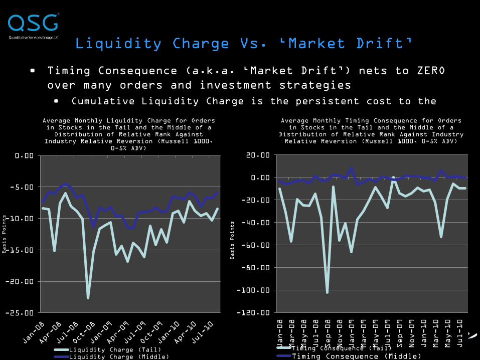
Liquidity Charge Vs. „Market Drift‟

• Timing Consequence (a.k.a. „Market Drift‟) nets to ZERO

over many orders and investment strategies

• Cumulative Liquidity Charge is the persistent cost to the

investor over time

-120.00

-100.00

-80.00

-60.00

-40.00

-20.00

0.00

20.00

Jan-08

Mar-08

May-08

Jul-08

Sep-08

Nov-08

Jan-09

Mar-09

May-09

Jul-09

Sep-09

Nov-09

Jan-10

Mar-10

May-10

Jul-10

Basis Points

Average Monthly Timing Consequence for Orders

in Stocks in the Tail and the Middle of a

Distribution of Relative Rank Against Industry

Relative Reversion (Russell 1000, 0-5% ADV)

Timing Consequence (Tail)

Timing Consequence (Middle)

-25.00

-20.00

-15.00

-10.00

-5.00

0.00

Basis Points

Average Monthly Liquidity Charge for Orders

in Stocks in the Tail and the Middle of a

Distribution of Relative Rank Against

Industry Relative Reversion (Russell 1000,

0-5% ADV)

Liquidity Charge (Tail)

Liquidity Charge (Middle)

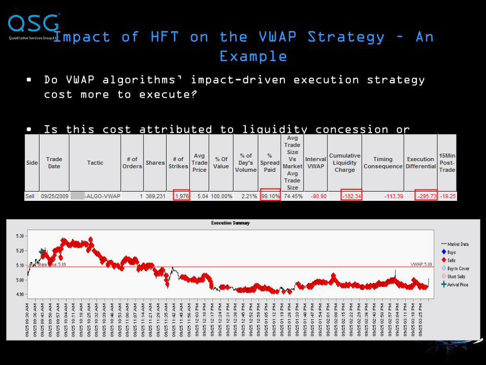
Impact of HFT on the VWAP Strategy – An

Example

• Do VWAP algorithms‟ impact-driven execution strategy

cost more to execute?

• Is this cost attributed to liquidity concession or

timing consequence?

VWAP Study - Sample Set

• QSG client data with algorithm flags

• 1/1/2009 through 8/05/2010

– Over 55 thousand orders

– More than $18B executed value

• VWAP and Arrival Price algorithms

• control group

– All orders ~1% ADV

• experimental group

– All orders ~1% ADV, < $10 stock price and $0.01

bid/offer spread

Results – Overall

OverallAlgorit

hm

Market Trade

Velocity

(strikes/min)

Avg

% of

DV

Avg

Fills

Per

Order

Avg %

Adverse

Tick

(Client)

Avg % Adv

Tick

(Market)

No Spread/Price

Constraint

Arrival 82 1% 100 19% 16%

VWAP 65 1% 63 28% 17%

$0.01 Spread &

<$10 Price

Constraint

Arrival 126 1% 111 12% 9%

VWAP 116 1% 145 26% 10%

-60.00

-50.00

-40.00

-30.00

-20.00

-10.00

0.00

Arrival VWAP Arrival VWAP

No Spread/Price Constraint $0.01 Spread & <$10 Price Constraint

Basis Points

Effect of Stock Price and Spread Size on Shortfall Decomposition for VWAP and

Arrival Price Algorithmic Orders of Size 1% ADV

Liquidity Charge

Results - IRR Factor Quartile Screen

OverallAlgorit

hm

Market Trade

Velocity

(strikes/min)

Avg

% of

DV

Avg

Fills

Per

Order

Avg %

Adverse

Tick

(Client)

Avg % Adv

Tick

(Market)

No Spread/Price

Constraint

Arrival 92 1% 95 19% 16%

VWAP 72 1% 73 27% 17%

$0.01 Spread &

<$10 Price

Arrival 147 1% 118 13% 9%

-60.00

-50.00

-40.00

-30.00

-20.00

-10.00

0.00

Arrival VWAP Arrival VWAP

No Spread/Price Constraint $0.01 Spread & <$10 Price Constraint

Basis Points

Effect of Stock Price and Spread Size on Shortfall Decomposition for VWAP and Arrival Price Algorithmic Orders of Size 1% ADV,

Ranked in the Top/Bottom Quartile of IRR over R1K on the Trade Date

Liquidity Charge

Results with IRR Factor Quartile Screen (Normalized)

0

0.2

0.4

0.6

0.8

1

1.2

1.4

1.6

1.8

Arrival VWAP Arrival VWAP

No Spread/Price Constraint $0.01 Spread & <$10 Price Constraint

Bid/Offer Spread Units

Effect of Stock Price and Spread Size on Spread-Adjusted Liquidity Charge for VWAP and Arrival Price Algorithmic Orders

of Size 1% ADV, Ranked in the Top/Bottom Quartile of IRR over R1K on the Trade Date

Spread-Adjusted Liquidity Charge

How Prevalent is HFT in the Dark?

• Top 4 pools allow HFT flow, Bottom 4 do not

Source: Rosenblatt Securities

Daily Volume

(Millions)

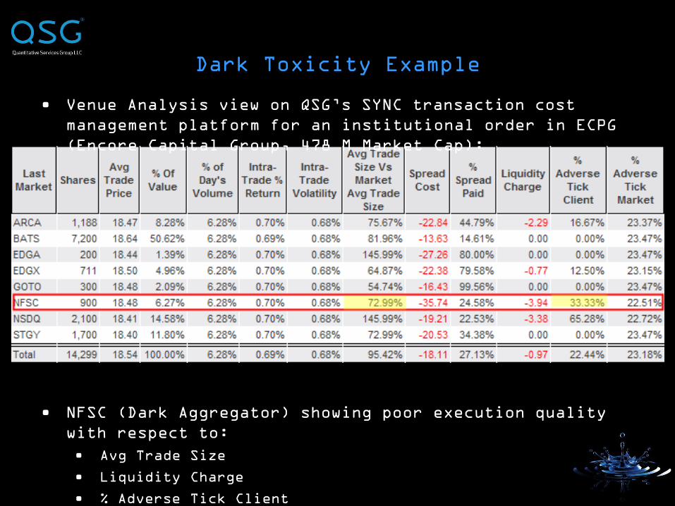
Dark Toxicity Example

• Venue Analysis view on QSG‟s SYNC transaction cost

management platform for an institutional order in ECPG

(Encore Capital Group, 478 M Market Cap):

• NFSC (Dark Aggregator) showing poor execution quality

with respect to:

• Avg Trade Size

• Liquidity Charge

• % Adverse Tick Client

Dark Toxicity Example

• ECPG on June 9th, 2010, 2:20:0 PM – 2:30:00 PM EST

• Midpoint Spread Dark Seller residing in all pools (via

an Aggregator) with a low limit price of $18.45

1

2

3

4

(1)The bid side of

the book is taken

out by visible

executions at

$18.46(2) Milliseconds

later, the

offering side of

the book is walked

down $0.11(3) The Dark Sell

order is

executed at a

B/D‟s internal

dark book at

$18.455(4) Within 5

seconds the

offering side

moves up $0.06

and within 10

seconds it is up

$0.18 from the

execution

9 ½

min

30

sec

Dark Aggregator Analysis

• Same methodology can be applied across dark execution

channels to measure signaling risk, toxicity and

quality of execution

– Comparison of 3 B/D Dark Aggregators

• $1B – $10B cap stocks

• 5% - 25% ADV

– Execution quality measures used:

• Implementation Shortfall

• Liquidity Charge

• 15-Min Post Trade Price (Adverse Selection)

• 20% Participation-Weighted VWAP

Dark Aggregator Analysis

-35

-30

-25

-20

-15

-10

-5

0

5

Dark Aggregator 2 Dark Aggregator 1 Dark Aggregator 3

Basis Points

Execution Quality Measures By Dark Aggregator

Arrival Price Shortfall (bps) Liquidity Charge (bps)

Dark Aggregator Analysis

-12

-10

-8

-6

-4

-2

0

2

4

Last Print

5Min 10Min 15Min 30Min 60min

Basis Points

Average Post-Trade Reversal By Dark

Aggregator

Dark Aggregator 2 Dark Aggregator 1

Dark Aggregator 3

Algorithm

% Value

Executed

Off-

Exchange

%

Liquidity

Charge

From Off-

Exchange

Dark

Aggregator 167% 65%

Dark

Aggregator 246% 46%

Dark

Aggregator 351% 74%

Conclusions

• VWAP algorithms show increased parceling

activity and increased adverse tick execution in

stocks below $10 in Price having $0.01 Bid/Offer

Spreads when compared to Arrival Price

algorithms

• Costs attributed to Liquidity Charge and

Execution Differential also increased, but

Liquidity Charge is more pronounced, especially

when screening trades by the Industry Relative

Reversal ranking

• Increased adverse ticks and Liquidity Charges

suggest disadvantages at the micro structural

level

• Methodology can be applied to next-generation

These materials are confidential. Distribution is Prohibited.

© 2010 Quantitative Services Group LLC. All Rights Reserved.

The examples in this presentation are for information purposes only and do not constitute investment advice or any recommendation to

transact. Investors should consider the appropriate professional advice before making an any investment decision.