‘ I I

HIGH FREQUENCY ACCELEROMETER CHARACTERIZATIONS* I Vesta I. Bateman Bruce D. Hansche Otis M. Solomon -- h n m

.--+.. Design, Evaluation & Test Technology Center .- i ‘f ; : ,-3 Sandia National Laboratories -.”. .4

P. 0. Box 5800 MS0555

Albuquerque, NM 87185-0555 (505) 844-0401

A laser doppler vibrometer (LDV) is being used for high frequency characterizations of accelerometers at Sandia National Laboratories (SNL). A LDV with high frequency (up to 1.5 MHz) and high velocity (10 d s ) capability was purchased from a commercial source and has been certified by the Primary Electrical Standards Department at SNL. The method used for this certification and the certification results are presented. Use of the LDV for characterization of accelerometers at high frequencies and of accelerometer sensitivity to cross-axis shocks on a Hopkinson bar apparatus is discussed.

. .

INTRODUCTION l e The Mechanical Shock Laboratory at Sandia National Laboratories (SNL) has developed a

Hopkinson bar capability to characterize accelerometers for both in-axis .and cross-axis response. A diagram of the Hopkinson bar I configuration for in-axis accelerometer characterizations is shown in Figure 1. This capability is being used to characterize accelerometers for SNL and other government agencies and for, development of new accelerometers and mechanical isolators for accelerometers as Cooperative Research and Development Agreements (CRADA’s) with transducer manufacturers. Usually, strain gages mounted on the Hopkinson bar have been used as the reference measurements. A method for calibrating the Hopkinson bar strain gages has been

* developed Cl]. However, as the frequency bandwidth for the accelerometer characterizations has been .extended, another reference measurement has become necessary. A laser doppler vibrometer (LDV) has been chosen as the reference measurement for the high ‘frequency accelerometer characterizations. and for cross-axis accelerometer characterizations. The manufacturer’s specifications for the LDV indicate a frequency bandwidth of up to 1.5 MHz and a velocity range of 10 d s , but there is no commercially available technique to certify or characterize the LDV. This pauer describes the dvnamic characterization of the LDV using

,

This work was supported by the U.S. Department of Energy under DE-AC04-94AL85000. *

I

Programming Material \ I:

Accelerometer

Air Gun

f I

Beryllium Hopkinson Ear

Figure 1: Hopkinson Bar Configuration for In-Axis Accelerometer Characterizations

optical and electrical inputs to the device that are substituted for the interferometric signal usually created by the test object. Since the wavelength of the laser is known to one part in lo6, certification accuracy is conceptually limited only by the accuracy of the electronic frequency generators and demodulators. An arbitrary waveform generator (AWG) is used to create the dynarnic signal that is input to.the LDV. Since the electrical signal in the LDV is frequency modulated with a center frequency of 40 MHz and a dynamic range of 32 MHz, the AWG must have a capability of varying a sine wave from 8 MHz to 72 MHZ at slew rates representing the 1.5 MHZ velocity response capability of the LDV. The results of the LDV characterization are presented and include the LDV uncertainty assigned by the SNL Primary Electrical Standards Department. The use of the LDV as a reference measurement in the characterizations of accelerometers for both high frequency characterizations of in-axis response and cross-axis measurements (out-of axis response) is discussed.

.. LDV CERTIFICATION COWIGURATION

A block diagram for the LDV is shown in Figure 2, where it can be seen that the optical signal is transformed into a frequency modulated electrical signal and then demodulated. This LDV is commercially available from Polytec PI*. .Model OFV-3000 controller and Model OW-302 sensor head have been certified in the.configuration shown in Figure 3. The reference frequency, fm, is 40 MHz for this device. A Tektronix Model AWG 2040 arbitrary waveform generator ’ provided the electronic certification signal. A Meret Model MDL 259-20-SMA laser diode converted&e AWG 2040 electrical output to an optical signal suitable for input to one of the detectors inside the LDV. The other detector was blocked with a piece of black tape. Only one detector is shown in the diagrams in Figures 2 and 3 although there are actually two detectors that are summed internally to the LDV. The LDV.electrically demodulates the output of the interferometer to estimate velocity. The velocity output of the LDV at the BNC connector on the front panel was measured with a Tektronix Model 11402 or Model DSA 602A digitizing oscilloscope with a Model 11A34 amplifier.

All equipment used for the LDV certifications was calibrated according to either manufacturer’s procedures or military calibration procedures. and their uncertainties (30 or coverage factor of * Reference to a commercial product implies no endorsement by SNL or the Department of Energy nor lack of suitable substitute.

. . . -I . ,. .

T f i S, = Wavelength h, accurate to one part in IO6. Bragg Cell AiCOSq +fm r\

r Doppler shifted %= A p s ( q + 2vl I.)

FM Demodulator : (Frequency to Voltage -i Convertor)

. V=V,+Kv(t)

Frequency f, = CJ h Modulator -

Figure 2: Normal Operating Block Diagram for LDV

F

4

Reference Frequency f, Generator: fm

Detector r

Recombined beam, s, +s,, I = < (S, + SJ2>

Detector

v = v,, + V,COS(s, - 2vl A)

FM Demodulator (Frequency to Voltage -i Convertor)

v = (31/2)€, nominal lv= I d s

G * Signal Generator .

Figure 3: Certification Configuration for LDV

Light Emitting DiodeGED)

Tektronix AWG2040 arbitrary waveform generator: swept sin to check rise time, slew rate. 40- f 32ME.Iz, up to 1.5 MH-z bandwidth (0.3 p risetime) of dynamic velocity. 1-1

Intensity modulated beam injected in place of Doppler interferometry beam

Table I: Equipment Used for LDV Certification

Function Frequency Voltage Voltage

Manufacturer Model Tektronix AWG 2040

Uncertainty 1 ppm 0.6 % 0.6 %

11A34 Laser Diode

Freq. Spectrum Frequency

Meret MDL259-20-SMA

Hew let t- 8590A Packard Hewlett- 5371A Packard

~

NA

NA

1 PPm

Identification E8341 5008

E8799

20161A s/N 119 E7294

E8635 I I

k=3) appear in Table I. As an additional check, the frequency of sine waves from the AWG 2040 was measured with a Hewlett-Packard Model 5371A frequency and time interval analyzer. At 8, 40 and 72 MHz, the signal was within 1 ppm of its setting. Both the LDV reference frequency (40 MHz) and the output of the laser diode through the LDV detector (with certified input frequencies) were also measured and found to be within .1 ppm of the frequency setting of the AWG 2040. Additionally, all warranteed specifications for the AWG including a rise time capability of 2.5 ns were verified in an AWG certification. The rise time, t, capability may be converted to bandwidth using [2]

.

t, = 0.35 / f,, a

where f,, is the single pole bandwidth, so the AWG has a bandwidth of 140 MHz. Thus, the AWG has a capability of varying a 40 MHz sine wave from 8 MHz to 72 M H z at frequencies exceeding the 1.5 IvlHz velocity response capability of the LDV.

A Hewlett-Packard Model 8590A spectrum analyzer was used to check for harmonics and interference signals. At amplitudes of 0.5 and 1 volt peak and frequencies of 8, 40 and 72 MHz, the AWG 2040’s fundamental was about 50 dBm.above its second harmonic; the detector’s fundamental was about 30 dBm above its second harmonic. To convert dBm to RMS volts with a 50 Q impedance that dissipates the power, the conversion formula is [3]

Pdnm = 2010g(V,,, / V,,, ) = 20log(VmS / 0.2236) .

Since a 1 volt peak value is 0.707 volts RMS or 10 dBm and the second harmonic of the AWG 2040 was 50 dBm less than the-fundamental, the second harmonic value is -40 dBm or 2.2 mV RMS. The -30 dBm for the second harmonic at the detector corresponds to 22.0 mV RMS. Voltage time histories of the signals showed no signs of amplitude clipping for these measurements. From these measurements, it was concluded that the effect of harmonic distortion in the AWG and the diode/detector was minimal.

The repeatability of the Tektronix Model 11402 digitizing oscilloscope with a Model llA34 amplifier was checked by measuring the output of a DC calibrator over a 24 hour period at -2 V and +2V. Both of the standard deviation of the means were less than 0.05% which indicates that the 0.6% uncertainty for voltage measurements listed in Table I is conservative.

CERTIFICATION PROCEDURE

A complete certification of the LDV would include static (constant velocity) and dynamic input signals. A constant sine wave input (constant velocity) to the LDV could be used for the static certification; however, a static certification does not accurately reflect the LDV’s dynamic performance. The LDV velocity output incorporates an offset limiter circuit that removes the collective DC drifts of the various electronic components and still gives the velocity output at the low frequency limit of 0.1 Hz. Thus, if a surface moves towards the LDV at a constant velocity, the velocity output will, at first, represent the speed but will fall off to zero volts in a time equal to the limiter’s response.

The dynamic portion of the LDV certification was fourfold short duration haversine pulses with various repetition rates, a rise time measurement using ramped signals, a bandwidth measurement with sinusoidally varying velocity, and a verification of the. slew rate specification using small signals up to 1.5 MHz. AU signals are frequency modulated (FM) signals created by.the AWG. An example of how the signals were created is given for the short duration haversine pulses. Although both RMS and peak measurements of the LDV output were made, in most cases, the results shown in this paper are for peak measurements because the primary ,application of interest is for shock (transient) measurements.

CERTIFICATION RESULTS

FM signals modulated by haversine pulses with short durations were also input to the LDV because haversine pulses are similar to pulses often encountered in shock testing. The haversine was programmed as 1. - cos(a t) and -(1 -. cos(a t)), so positive and negative haversine pulses alternated at the test frequencies. Two frequencies were used: 33.3333 kHz (15. ps wide per . pulse) and 66.6666 H z (7.5 ps wide per pulse). The form of a FM signal is [4]:

$ ( t ) = 27ckf x(t)dt ‘0

(3)

x ( t ) = the modulating (message) signal

The center frequency of the FM signal is a,. The instantaneous phase is @(t) . The derivative of $(t) is proportional to the instantaneous frequency deviation. The constant k is the frequency deviation constant with units of hertz per unit of x(t ) .

5

Table II shows an equation file to create a FM signal for a haversine pulse train with the Tektronix Model AWG2040 arbitrary waveform generator. The DC value of the pulse train is zero. Comment lines begin with the "#',symbol. Constant kl defines the center frequency of the FM signal. Constant k2 defines the haversine amplitude. Constant k3 controls the repetition rate of the pulse train and is set equal to twice the repetition rate of the pulse train. Constant k4 defines the frequency deviation constant of the FM signal. Line 11 defines the range or time interval of the positive haversine. Line 12 defines the FM signal for the positive haversine. Line 14 defines the range of the negative haversine. Line 15 defines the FM signal for the negative haversine. Note that the integral of the haversine 1 - cos(k,t) over the time interval Oto t is t - sin(k,t) / k, . To verify the fidelity of the FM signal created by the AWG, the signal could be demodulated with a FM receiver other than the LDV. Since a F M receiver was not available, digitizing the FM signal and then demodulating it was considered, but this task was not performed .

because of lack of time.

Line Number

1 2 3 4

Table 11: Equation File for Tek Model AWG2040

Command

# FM signal for haversine pulse train # Center frequency = 40 MHz kl=2*pi*40e6 # Haversine amditude = 9 V

5 6 7 8 9

k2=9 # Period of haversine pulse train = 30 us k3=2*pi*66.6666e3 # Frequency deviation constant k4=2*~i*32e6/20

10 11 range(Ous, 15us) 12 13 14 ranie(15us.30~~)

# FM signal for positive haversine

sin( k 1 * t+k2* k4* (t-sin(k3 * t)/k3)) # FM signal for negative haversine

. .

I' . 15 I sin(kl*t-k2*k4*(t-0.000015-sin(k3*t~/k3~) I

Table 111 shows the measurement results for the haversine pulses. For each measurement, there are: the frequency (repetition rate of the positive and negative haversine pulses); the theoretical peak-peak response amplifude in volts; the peak-to-peak value of the LDV output as measured by the Tektronix DSA 602A, and finally the percent difference calculated as the percent of full scale. Other measurements were also made of the RMS values of both the LDV and the Tektronix AWG 2040 but are not shown here. For the data at 33.333 kHz and at 66.6666 kHz, the largest deviation of the peak-to-peak of the response from the theoretical peak-to-peak is 0.92 V at -10 V. These deviations are similar to the deviations found for the slew rate tests described below for the 1000 m d s N range.

The operating range of the Polytec Model OVD-02 velocity output module is limited to 1.5 MHz. Equation (1) indicates for a 1.5 MHz bandwidth, the risetime is about 0.23 ps. To study the risetime of the LDV, the risetime of the Tektronix AWG 2040 was varied from 10 to 0.1 ps for

. pulse inputs. The upper and lower levels of the .pulses correspond to modulating frequencies of 60 MHz and 20 MHz, respectively. These modulating frequencies should produce voltages- of 6.25 V and - 6.25 V at the velocity BNC connector. Table N summarizes the risetime data. The data in Table IV show that the risetime for a step of 12.5 V peak-to-peak is between 0.8 and 0.16 ps, which is consistent with the LDV minimum rise time specification. The main degradation of the velocity data is the overshoot due to the ringing after the pulse transition.

AWG Risetime (ps) 8.00

- 4.00

Table 111: Measurements of LDV Response to Short Duration Haversine Pulses.

Measured Risetime (p) Measured Overshoot (%) 7.93 0.26 4.04 1.27

Table IV: Risetime Measurements

0.16 0.08

0.32 16.46 0.3 1 18.35

I 0.80 I 0.8 1 I 3.17 I

Next, measurements were made to determine the bandwidth (BW) for the LDV. The operating range of the Polytec Model OVD-02 velocity output module is limited to a BW of 1.5 MHz and a slew rate of 200,000 g, and both conditions must be met simultaneously. The operating range polygon for the Polytec Model OVD-02 shows that the 1.5 MHz BW specification applies only to

7

small signals and that large signals with frequency content above 31 lcHz are slew rate limited. A discussion of BW specifications in contained in [5]. According to the operating range polygon at 1.5 NHZ, the maximum signal which is not slew rate limited is approximately 0.25 V peak. The BW was-’checked at modulation frequencies that would theoretically produce 1 V RMS output (over five times larger than 0.25 V peak) and with FM signals modulated by sinusoidally varying velocities at various frequencies and amplitudes. Their parameters are: 1 V RMS at 33.3333 kHz; 1 V RMS at 1.65 NHZ; 7 V RMS (10 V peak) at 1.5 MHz;. and 7 V RMS (10 V peak) at 1.3 MHz. All waveforms were correctly reproduced, so the LDV meets or exceeds its specifications for BW. Table V shows the results of these measurements. The first two columns in Table V show the frequency and RMS of the modulating signal in the AWG 2040. Column 3 shows the measurements acquired with the DSA 602A from the velocity output BNC connector on the LDV. According to these data, the -3 dB (0.707 gain) frequency is about 1.65 MHz. These measurements indicate that the instrument exceeds its specifications. Fipre 4 is a plot of the RMS voltage versus frequency where the RMS voltage increases slightly from about 500 kHz to about 1.5 M H z and then decays rapidly.

Table V: BandMdth Measurements at 1000 d s N .

1.2

1 .o

0.8 v s cn

0.6

0.4

0.2 I I

0 lo00 2000

Frequency (kHz)

Figure 4: Bandwidth for LDV Range 1000 mm/sN. (Measured RMS Voltage versus Frequency)

8 I

Finally, the slew rate specification for the LDV was checked. The Polytec Model OVD-02 velocity output module is limited to 1.5 MHz and slew rates of 200,000 g. According to the specifications of the vibrometer, both conditions must be met simultaneously. The slew rate limits the maximum full scale range to 31 kHz. The relationship between slewing time, tslew,-’and bandwidth, fb , is [2]

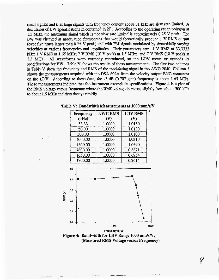
The slewing time, tslew, for 31 kHz is 10 ps. Figures 5 to 7 show a typical simulated velocity pulse as measured with a Tektronix Model DSA 602A digitizing oscilloscope with a Tektronix Model llA34 amplifier (1 M?2 input impedance and 300 MHz bandwidth), at the velocity output BNC connector on the front of the LDV. The pulse transitions from one level to another level in 10 ps. The lower and upper levels are varied to characterize the instrument over its full range. The pulse in Figure 5 switches between modulation frequencies of 10 MHz and 70 MHz. The amplitude of the overshoot and subsequent ,oscillations are larger at the negative voltages than at the positive voltages. This behavior was typical of the LDV performance on the 1000mmlsN range: the overshoot and subsequent oscillations in the velocity output are larger for modulating frequencies less than 40 M H z than for modulating frequencies above 40 MHz. .

Figure 5: Simulated Velocity Pulse Output from the LDV. (500 MHz Sample Rate)

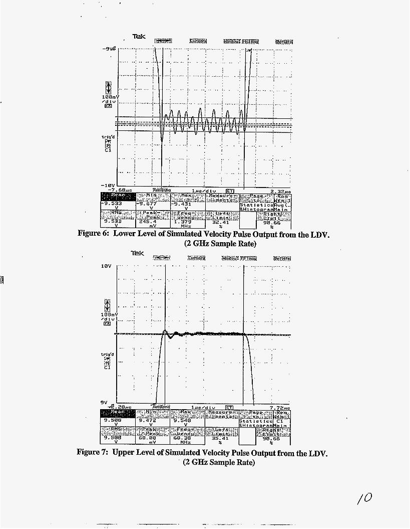
Figure 6: Lower Level of Simulated Velocity Pulse Output from

. . . . . . . . . . . . . . . . . . .

10v

[# 100m /diu El

trig'd

c1

a 9v

. . . . . . . . . . . . . . . . . . . . . . . . . . . . . .

. . . . . . . ......................

(2 GHz Sample Rate) - T i r-3 z: -"-'"

.%'A. .x I . . r. . ~ . G O r n W.Zl.Emm K<RrnS . . . . . . . . . . . . . . . .. ," ...................... " : ' -.I :

the LDV.

Figure 7: Upper Level of Simulated Velocity Pulse Output from the LDV. ' (2 GHz Sample Rate)

Table VI shows measurements of the velocity output voltage for the 1000 d s N range. The first two columns are the frequency of the modulating signal and the corresponding theoretical voltage that should appear at the velocity output BNC connector. The third column is the voltage that deviates the most from the theoretical voltage over about a 5 ps analysis interval. The fourth column is the difference between the largest deviation and the theoretical value as a percent of full scale. The largest percent difference is 8% of full scale at 8 MHz. The second largest percent difference is 2.9% at 68 MHz.

4

Table VII shows measurements of the velocity output voltage for the 125 d s N range. The information in the columns is the same as for Table VI. The largest deviations from the theoretical values are smaller than those for the 1000mmlsN range. Tables Vm shows the measurements of the velocity output voltage for the 25 mm/sN range. The worst deviation from the theoretical value, 2.7% of full scale, occurs at 40.8 MHz.

LDV CERTIFICATION UNCERTAINTY

The main contributors to the uncertainty of our certification of the velocity output of the LDV . are: (1) the frequency of the FM signal generated by the Tektronix Model AWG 2040 arbitrary

waveform.generator (from Table I); (29 the uncertainty of the voltage measurements with the Tektronix Model 11402 or Model DSA 602A digitizing,waveform recorder with a Model 11A34 amplifier (from.Table I); (3) the residualsaof a linear fit of the mean output velocity voltage to the theoretical output velocity voltage computed from the frequency.of the modulating signal in the

, AWG 2040 (not shown); and (4) the difference between the theoretical output voltage and the worst deviation from the theoretical output voltage. The total uncertainty for a particular velocity . is the RSS of the values from sources 1 to 3 plus the-value of source 4 The random components I

' (1) to (3J are combined as the-square root of the sum of the squares (RSS). Component (4) is a worst case error which is not combined as RSS. For the 1000 mm/sN range, the total uncertainty'

.

4 , ..

Table VI: LDV Measurements for 1000 m d s N Range with 8 ~ L S Risetime.

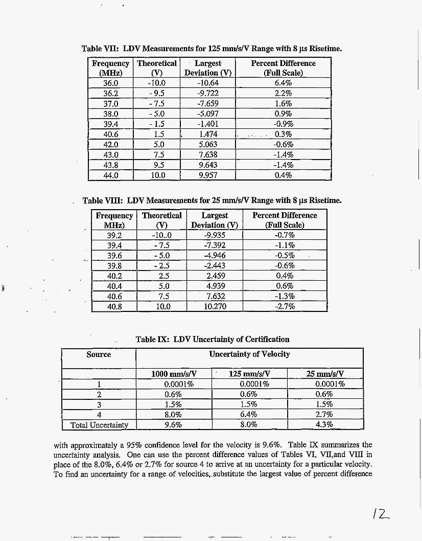
Table VII: LDV Measurements for 125 d s / V Range with 8 p Risetime.

Source

1 2 3 4

Total Uncertainty

. Table VIII: LDV Measurements for 25 d s N Range with 8 ps Risetime.

.. ,

Uncertainty of Velocity

1000 mIn/sN ’ 1 2 5 d d V 25 d s N 0.0001 % 0.0001 % 0.0001 % 0.6% 0.6% 0.6% 1.5% 1.5% 1.5% 8.0% 6.4% 2.7% 9.6% 8.0% 4.3%

with approximately a 95% confidence level for the velocity is 9.6%. Table M summarizes the uncertainty analysis. One can use the percent difference values of Tables VI, Vll,and VIII in place of the 8.0%, 6.4% or 2.7% for source 4 to arrive at an uncertainty for a particular velocity. To find an uncertainty for a range of velocities,.substitute the largest value of percent difference

I

I

(full scale) for the restricted velocity range for source 4. For example, for the 1000 d s N range, the uncertainty for velocities corresponding to voltages ranging from -9.375 to 10 V is 4.5%. Similarly, for the 125 d s N range, the uncertainty for velocities corresponding to voltages ranging from -9.5 to 10 V is 3.8%.

ACCELEROMETER CHARACTERIZATIONS USING A LASER DOPPLER VIBROMETER

The LDV is being used to make measurements at the end of beryllium Hopkinson bars where accelerometers are mounted for characterization. The high frequency response of the LDV and the, high wave speed for beryllium allow characterizations of accelerometers for the frequency range of DC-50 kHz. The LDV is also being used to make measurements.of the lateral motion due to Poisson's effect of a Hopkinson bar. The lateral motion is then subtracted out of the accelerometer response for accelerometers mounted on the side of the Hopkinson bar. These accelerometers are subjected to stress waves in their non-sensitive axis or cross-axis direction. The accelerometers correctly respond to the lateral motion, so this motion must be subtracted out to .derive the cross-axis response. No sensor, other than the LDV, can detect this lateral motion at frequencies up to 1.5 MHz. Other researchers [6,7,8] are using a LDV to characterize strain gages. However, the LDV used in these studies has one-tenth the velocity range of the LDV certified in this paper and does not have the high frequency capability of DC-1.5 MHz.

' CONCLUSIONS

The dynamic parameters (short duration haversine pulses, rise time, bandwidth and slew rate) for the LDV have been successfully certified. The measurements in this paper provide information about the LDV that has not been previously known. The largest uncertainty occurs on the largest velocity scale of 1000 d s N and at only one point. The largest uncertainty corresponds to the condition where the testobject is moving away from the LDV. FOF accelerometer measurements, the LDV is customarily used for measurements when the target is moving towards the LDV. Additionally, the largest uncertainty occurs due to overshoot. Whenthe LDV is used over 90% of its range, this LDV has a 2-3% uncertainty for all specified frequencies and velocities. The uncertainty decreases for decreasing velocity scales. The LDV provides a reference velocity measurement for velocities up to 10 m/s and for frequencies up to 1.5 MHz. This reference measurement provides information,in a bandwidth that is not available from strain gages that. are generally considered to have a bandwidth of no greater than DC-40 kHz. Future work should include digitally demodulating the FM signal from the AWG and comparing it with the LDV output. Additionally, the LDV should be used to characterize strain gage response for frequencies up to 1.5 MHz.

.

DISCLArmER

This report was prepared as an account of work sponsored by an agency of the United States Government. Neither the United States Government nor any agency thereof, nor any of their employees, makes any warranty, express or implied, or assumes any legal liability or responsi- bility for the accuracy, completeness. or usefulness of any information, apparatus, product, or process disclosed, or represents that its use would not infringe privately owned rights. Refer- ence. herein to any specific commercial product, process, or service by trade name, trademark, manufacturer, or otherwise does not necessarily constitute or imply its endorsement, recom- mendation, or favoring by the United States Government or any agency thereof. The views and opinions of authors expressed herein do not necessarily state or reflect those of the United States Government or any agency thereof.

~~

ACKNOWLEDGMENTS

The authors gratefully acknowledge the assistance of Adrian C. Goding, Polytec PI, throughout this project. He provided valuable technical knowledge and insight of the LDV operation that

. allowed us to complete this project. The authors also gratefully acknowledge Bob Nichols of White Sands Missile Range who encouraged them to pursue this work. The authors thank Dave Evans and Bev Payne of the National Institute of Standards and Technology for sharing their experiences with earlier models of the Polytec LDV [9].

REFERENCES

1. Bateman, V. I., W. B. Leisher, F. A. Brown, and N. T. Davie, “Calibration of a Hopkinson Bar With-aTransfer Standard,” Shock and Vibration Journal, Vol. 1, No. 2, 1993, pp. 145-152.

2. Feucht, Dennis L., Handbook of Analog Circuit Design, Academic Press, 1990 pp. 318-322.

3.. Witte, Robert A. Spectrum and Network Measurements, Prentice-Hall, 199 1, pp. 1 1-2 1.

4. Carlson, A. Bruce, Communication Systems, 3rd ed., McGraw-Hill, New York, 1986, pp. 23 1-243.

5. Frederiksen, Thomas M., Intuitive IC Op Amps, R. R. Donnelley, 1984, pp. 28-35.

6. Umeda, Akira, and Kazunaga Ueda, “Characteristics of Strain Gage Dynamic Response Using Davies’ Bar and Laser Interferometry,” Proceedings of the VIlh International Congress on Experimental Mechanics, Society of Experimental Mechanics,’ June 8-1 1, 1992, Las Vegas, NV, pp. 837-842.

7. Ueda, Kazunaga and Akira Umeda, “Dynamic Response of Shock Accelerometers Measured by Davies’ Bar Technique and Laser Interferometry,” Proceedings of the VIPh International Congress on Experimental Mechanics, Society of Experimental Mechanics, June 8- 1 1, 1992, Las Vegas, NV, pp. 1666-1673.

8. Umeda, Akira, and Kazunaga Ueda, ‘.‘Measurement of the Strain Gage Dynamic Transverse and Longitudinal Sensitivity Using *Pulse Elastic Waves and Laser Interferometry,” Proceedings of the lo‘” International Congress on Experimental Mechanics, Society of Experimental Mechanics, July 18-22, 1994, Lisbon, Portugal, pp. 319-324.

9. Evans, David J., Daniel R. Hynn, and Donald C. Robinson, “Development of a Mechanical Shock Calibration System: Technical Progress Report,” submitted to Physical Standards Division of the Measurement Standards Department at SNL, Albuquerque, NM from Automated Production Technology Division of the Manufacturing Engineering Laboratory at the National Institute of Standards and Technology, Gaithersburg, MD, January 1991.