High-Energy 2-µm Doppler Lidar for Wind Measurements

Grady J. Koch*a, Jeffrey Y. Beyonb , Bruce W. Barnesa, Mulugeta Petrosc, Jirong Yua , Farzin Amzajerdiana, Michael J. Kavayaa, and Upendra N. Singha

aNASA Langley Research Center, MS 468, Hampton, VA USA 23681 bCalifornia State University, Dept. of Electrical and Computer Engineering, Los Angeles, CA USA

cScience and Technology Corporation, 10 Basil Sawyer Drive, Hampton, VA USA 23666 *e-mail: grady.j.koch@nasa.gov, voice: 757-864-3850, fax: 757-864-8828

https://ntrs.nasa.gov/search.jsp?R=20080013367 2020-04-27T03:10:41+00:00Z

2

ABSTRACT

High-energy 2-µm wavelength lasers have been incorporated in a prototype coherent Doppler lidar to test component technologies and explore applications for remote sensing of the atmosphere. Design of the lidar is presented including aspects in the laser transmitter, receiver, photodetector, and signal processing. Calibration tests and sample atmospheric data are presented on wind and aerosol profiling.

3

1. INTRODUCTION

Recent advances in high-energy 2-µm solid-state laser technology have enabled lidar

applications for long range wind sensing. Wind profiling with 2-µm lidar has already shown merit

using low-energy (1-10 mJ) laser transmitters based on thulium.1,2,3 And the addition of stronger

energy lasers promises to boost the applicability of the coherent Doppler technique to farther

distances and higher altitudes. Comparable or higher pulse energy that the coherent Doppler lidar

described here has been demonstrated but at wavelengths of 1-µm from a neodymium laser and 10-

µm from CO2 lasers.4,5,6,7 The 2-µm based approach overcomes a disadvantage with the 1-µm lidar

in that the 2-µm wavelength offers a much higher level of eye safety. The 2-µm wavelength laser is

appealing over the 10-µm laser because the 2-µm laser is a solid-state medium of more convenient

and robust implementation than CO2 gas. A further advantage of the lidar described here is the

demonstrated capability of adding amplification stages to the laser for even more pulse energy that

might be required for a spaceborne lidar.8 Research at NASA is developing lidar technology for

satellite-based observation of wind on a global scale. The ability to profile tropospheric wind is a

key measurement for understanding and predicting atmospheric dynamics and is a critical

measurement for improving weather forecasting and climate modeling.9 Homeland security

applications have been proposed to provide wind data for accurate transport prediction of a plume

release of a nuclear, biological, or chemical agent.10

We report here on technology developments and lidar system demonstrations aimed at long-

range wind applications. A new laser composition of Ho:Tm:LuLiF is used that optimizes output

energy. The coherent heterodyne receiver is also discussed, including advances with an integrated

photodiode/preamp in a dual-balanced configuration. A lidar system testbed has been built from

4

these components and integrated with a real-time signal processing and display computer. This

testbed has been named VALIDAR from the concept of “validation lidar,” in that it can serve as a

component technology calibration and validation source for future airborne and spaceborne lidar

missions. VALIDAR is housed within a mobile trailer for field measurements.

2. LIDAR DESIGN

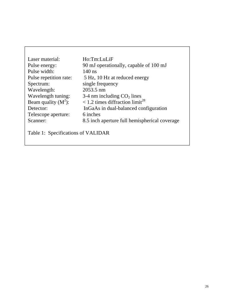
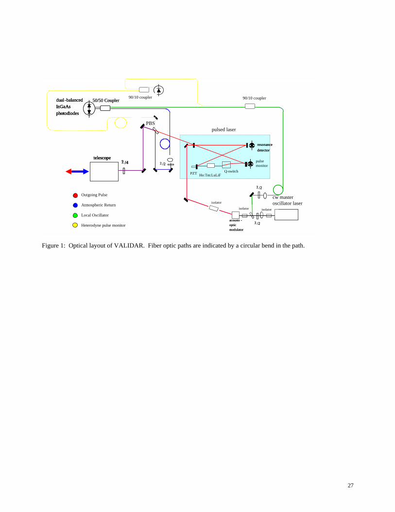
The optical layout of VALIDAR is shown in Figure 1 and a list of specifications is given in

Table 1. Transmitter and receiver subsystems are each described separately, with the transmitter

considered to consist of the pulsed laser, continuous wave (CW) laser, and the optics associated

with coupling the two. The receiver is considered to be the transmit/receive switch, telescope, and

photodetector. Not shown in Figure 1 is a scanner mounted through the roof of the trailer for

steering the lidar beam.

2.1. Laser Transmitter

The 2-µm wavelength is advantageous in a coherent Doppler lidar for several reasons.

First, it offers a high level of eye safety with a maximum permissible exposure of 100 mJ/cm2.11

Second, the 2-µm wavelength is strongly backscattered by aerosols in the atmosphere, from which

the Doppler shift indicates wind speed. Third, holmium solid-state lasers can produce a high level

of pulse energy at 2.05 µm.

5

A holmium laser material, with an activator of thulium, is used to generate the 2-µm

wavelength. The holmium/thulium composition has traditionally been used with host materials of

yttrium aluminum garnet (YAG) and yttrium lithium fluoride (YLiF), and Henderson et. al used a

flashlamp-pumped Ho:Tm:YAG laser in a Doppler lidar.12 The transmitter described here uses a

host material of lutetium lithium fluoride (LuLiF) pumped by diode laser arrays. LuLiF allows

more output energy than YAG or YLiF, while retaining high damage tolerance and a low level of

thermal lensing.13 An experiment in which YLiF and LuLiF crystals of the same holmium and

thulium concentrations were interchanged with the same diode pumping showed 20% more pulse

energy from the LuLiF crystal. The transmitter described here is of a single laser oscillator, but

considerable work has gone into oscillator-amplifier designs showing as much as 1-J of energy per

pulse.8 Other work has shown a laser oscillator that is conductively cooled, eliminating the water

cooling of the pulsed laser described here.14

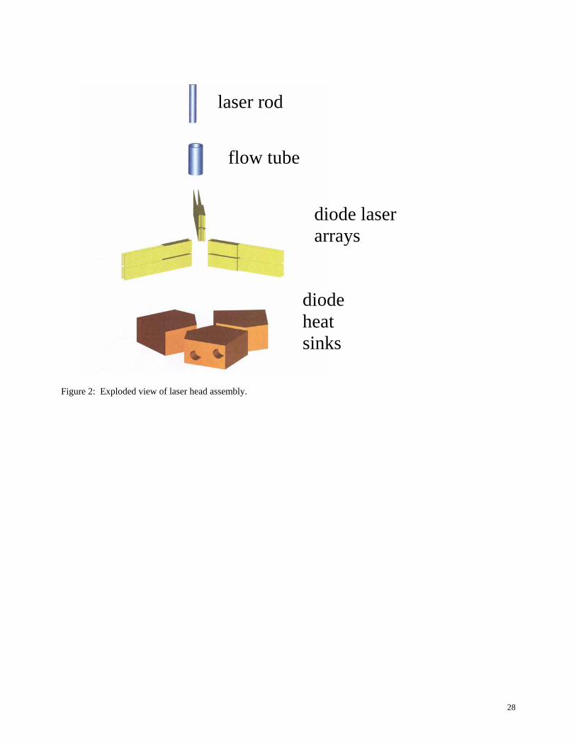
As diagrammed in Figure 2, the Ho:Tm:LuLiF rod is contained in a pump head using

conductively cooled laser diode arrays. Water cooling is used for the heat sink of the diode arrays,

but the laser diodes are not directly cooled with water. Six AlGaAs diode arrays side pump the

laser rod; each array has six bars that can provide up to 600 mJ near 792 nm in a 1-ms pulse. Three

sets of two diode arrays, side by side, are arranged 120o apart around the laser rod circumference.

The laser rod has a diameter of 4 mm and is encased in a 6-mm outer-diameter fused-silica glass

tube for water cooling of the laser rod; the coolant temperature is kept at 15 C. The 20-mm long

laser rod is doped with 6% Tm and 0.4% Ho. The resonator is in a ring configuration with a total

length of 2.0 m, with an acousto-optic Q-switch to spoil the laser cavity.

A continuous wave (CW) Ho:Tm:YLF laser serves as both an injection seed source and a

local oscillator. This laser was originally built by Coherent Technologies, Inc. for the Space

6

Readiness Coherent Lidar Experiment (SPARCLE).15 Approximately 10 mW of this CW laser is

split off and focused into a polarization maintaining optical fiber for the local oscillator channel.

Two channels of heterodyne detection are used: one for that atmospheric backscatter and one for

monitoring the outgoing laser pulse. To feed these two channels the local oscillator is split with a

fiber optic evanescent wave coupler. The heterodyne pulse monitor is required to create a reference

in time (from which to base range calculation) and frequency (from which to base Doppler shift

calculation). Taking the pulse monitor from the atmospheric backscatter channel was evaluated in

hope of using only one heterodyne detector and reducing the parts count. However, it was found

that the gain required on the atmospheric channel photodetector was too high for the pulse monitor,

creating a saturated and distorted pulse monitor. The time and frequency references from the

distorted monitor were often erroneous, creating time and frequency bias in the output data

products. We concluded that two photodetector channels are required with different gain settings.

The rest of the CW energy is used for injection seeding after being frequency shifted 105

MHz by an acousto-optic modulator (AOM). Such an offset sets an intermediate frequency

between the local oscillator and pulsed laser output. A series of three Faraday isolators are used

between the CW laser and the pulsed laser in order to prevent damage to the CW laser from a

counter-propagating laser pulse and to isolate the local oscillator channel from influences by the

laser pulse and AOM. If continuously left on, the AOM was found to generate residual amplitude

modulation and electromagnetic at its modulation frequency that interfered with the Doppler

signals. Hence, the AOM is shut off after the injection seeding takes hold and the laser pulse is

formed. The 0th order, non-shifted beam through the AOM is not used in the scheme diagrammed

in Figure 1. However, a configuration has been successfully tested to use the 0th order beam

coming through the AOM, with the AOM switched off after seeding, as the local oscillator. With

7

the AOM shut off all of the CW energy input to the AOM is available. This scheme may be

beneficial in designs where the CW master oscillator power is limited.

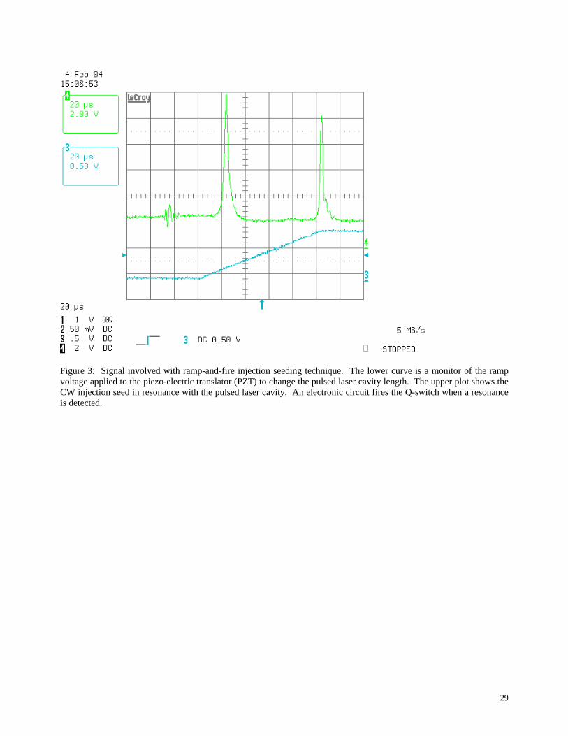
To ensure a single-frequency pulsed output by the injection seeding process, the pulsed laser

cavity is actively matched to the frequency of the injection seed by a ramp-and-fire technique.16 A

piezo-electric translator (PZT) mounted to a mirror of the pulsed laser is ramped by voltage, as

shown in Figure 3. An InGaAs photodiode circuit views the resonance of the injection seed with

the pulsed laser cavity, and resonance peaks occur when the pulsed laser cavity length matches the

injection seed frequency. A circuit senses the resonance and fires the Q-switch when this cavity

matching condition is determined. This results in a single-frequency output spectrum from the

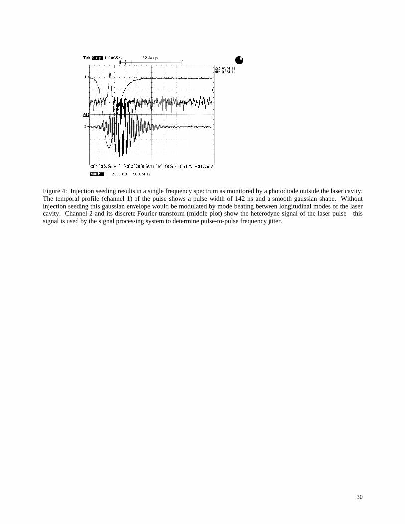
pulsed laser. Successful seeding can be determined by a smooth shape to the laser pulse, as shown

in Figure 4, and an approximate doubling of output power as the ring resonator is forced to run in a

single direction. The frequency difference between the output pulse and local oscillator, while

nominally at 105 MHz, jitters on a shot-to-shot basis by as much as several MHz. Statistics on

frequency jitter are presented in Section 2.4.

The Ho:Tm:LuLiF output wavelength can be tuned between 2050 to 2057 nm with the exact

wavelength selected by the injection seed. The gain peaks around 2053.5 nm which allows for the

easiest injection seeding. Another factor in selecting wavelength is the presence of CO2 and H2O

lines within the laser’s tuning range. Consulting with the HITRAN atmospheric database to avoid

these lines and find minimal absorption led us to select the operating wavelength at 2053.47 nm,

corresponding to a two-way atmospheric transmission from the ground to 8 km altitude of 87.2%.17

The presence of these absorption lines can also be exploited to measure gas concentration, with CO2

being of particular interest. A design very similar to the lidar system described here has been

reported for making CO2 differential absorption lidar measurements.18

8

2.2. Receiver

The basic design of the receiver is similar to those described in use with lower energy 2-µm

system.2,12 Differences with the design used here are in optical fiber rather than free-space routing

of optical signals and an improvement in the photodetector implementation using a dual-balanced

configuration. The use of optical fiber allows for a convenient and flexible implementation of the

devices in the optical path, such that they can be easily disconnected for replacement, diagnostics,

or trouble shooting.

The pulsed laser output is transmitted to the atmosphere via a 6-inch diameter off-axis

paraboloid telescope. After expansion by the telescope, the output laser beam can be pointed or

scanned by a scanner mounted through the roof of the trailer. The outgoing pulse and atmospheric

backscatter are separated by a polarization relationship imposed by the combination of a quarter-

wave plate and polarizing beam splitter.

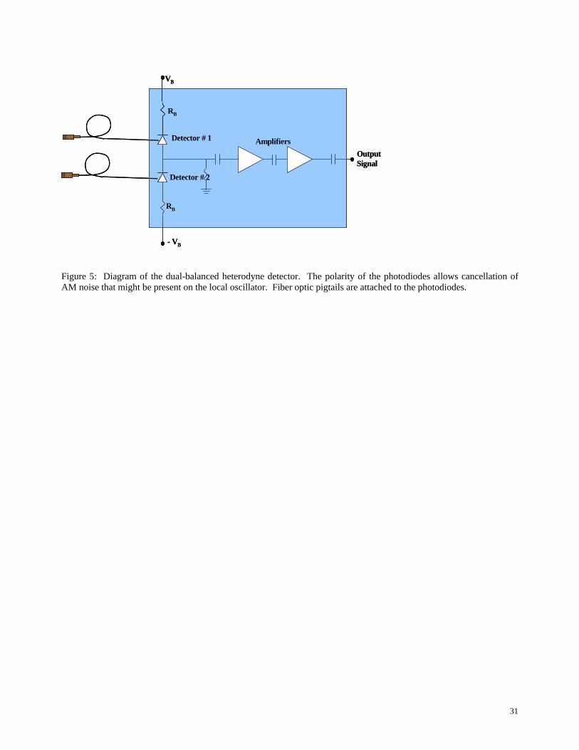
Heterodyne detection is provided by InGaAs photodiodes in a dual-balanced configuration

as diagrammed in Figure 5. Such a detector configuration has been thoroughly investigated for use

in telecommunications applications, but not well known for use in Doppler lidar.19 The dual-

balanced design is used here as it allows collection of all of the atmospheric backscatter and local

oscillator through a 50/50 evanescent wave coupler. A more typical design would be to use a single

photodiode with a coupler taking 90% of the atmospheric backscatter and 10% of the local

oscillator. The dual-balanced configuration has an additional benefit of canceling amplitude noise

that may occur in the local oscillator. A photodetector circuit is being used that combines the

9

photodiodes and amplifiers (in die form) integrated together in the same microelectronic package.

Such packaging reduces parasitic capacitance, thus improving performance where a wide bandwidth

is needed. A factor of 2.2 reduction in parasitic capacitance has been shown over a previous design

using discrete components integrated on a printed circuit board. The circuit used in VALIDAR has

a 200 MHz bandwidth, but circuits have been developed with 2 GHz bandwidth.20

2.3. Data acquisition and signal processing

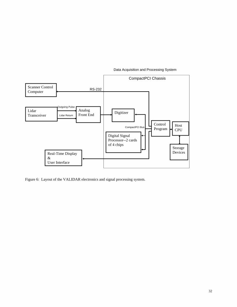
Processing of the lidar data is accomplished in real-time with the system diagrammed in

Figure 6. Real-time reduction of the heterodyne signal to wind and backscatter data products was

taken to be an important feature in order to accommodate future missions, such as from an aircraft

with the lidar operating autonomously, in which the transmission or storage of raw data might not

be possible.

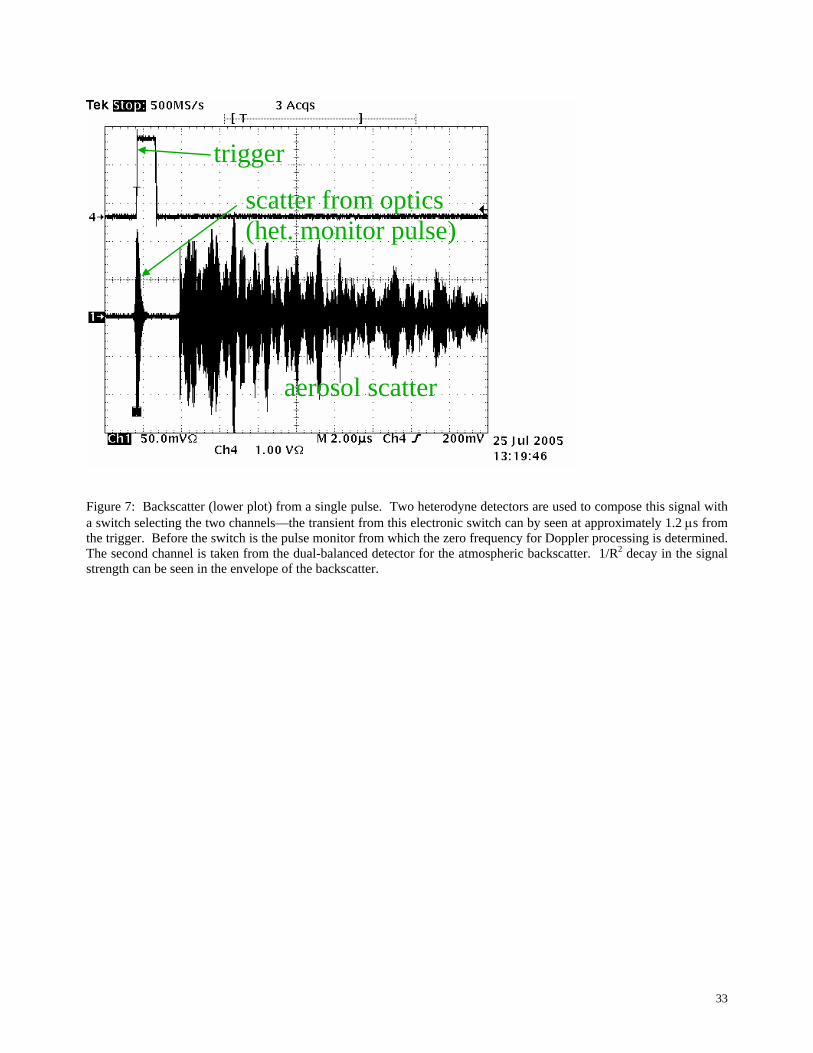
The heterodyne signal is conditioned by an analog front end that includes an anti-aliasing

filter and two different level of amplification switched in to bring the outgoing scatter pulse and

atmospheric return within the dynamic range of a digitizer. Sampling by the digitizer is at 500 Ms/s

and 8 bit resolution. An example of a single digitized heterodyne signal is shown in Figure 7 in

time domain.

Digitized data flows to an array of SHARC digital signal processors (DSP) for real-time

reduction of the heterodyne signal to wind and power data products. The DSP, digitizer, and

control software are hosted by a single computer over a PCI backplane. Control software includes a

program in which the user can set such parameters as number of sample points, number of pulses to

10

be averaged, scanner angles, and display preferences. An outline of the processing steps for an

acquisition along a single line of sight is given in the following:

Step (A): acquire

An individual pulse is digitized starting from a trigger generated by a monitor photodetector.

A user-specified number of samples is taken and separated into range bins with a typical setup

being 50,000 samples (corresponding to 15 km range) broken into 512 sample bins (corresponding

to 153.6 m). The first range bin, however, can be of a longer length of 1024 samples to isolate the

outgoing pulse scattered from the lidar optics. The scatter pulse is also called a monitor pulse

because it is used to monitor for frequency jitter that may occur in the injection seeding process.

Range bin information is converted to range in meters. A number of pulses is acquired for

averaging as specified by the user. As an option range bins may to overlapped to smooth the wind

measurements in range. For example, the atmospheric measurements shown later were made with

range bins overlapped by 50% to provide a data point every 76.8 m.

Step (B): FFT

The power spectrum of the data for each range bin is calculated by a fast Fourier transform

(FFT). A Hamming window may be applied as an option.

11

Step (C): monitor frequency determination

The frequency corresponding to the peak of the spectrum is estimated in the first range bin

containing the monitor pulse. This estimated frequency is compared to a user-specified frequency

range to check if the laser pulse was properly injection seeded. An unseeded pulse, which occurs

for less than 1% of the laser pulses, will have a maximum frequency estimate at a frequency

corresponding to the free spectral range of the pulsed laser cavity since multiple modes are beating.

Such a mode beating frequency is well away from the intermediate frequency and is easily filtered

by this step. If a bad pulse is detected it is discarded from the set so that it will not be included in

averaging.

Step (D): shift spectra

Taking the first pulse in the accumulation as the reference, provided it passed the test of the

above step, the spectra of the following pulses’ atmospheric returns are shifted in frequency to

remove the effects of pulse-to-pulse frequency jitter. The amount of shifting applied to each pulse

is determined from Step (C).

Step (E): averaging

12

The jitter-corrected spectra for each range bin are averaged among all the pulses acquired.

A typical configuration is to use 20 pulses for averaging.

Step (F): Doppler shift and power estimation

The frequency corresponding to the peak of the spectrum is determined for each range bin

and subtracted from the zero Doppler reference frequency. This result is used to determine the

Doppler shift. The power spectrum for each range bin is estimated by a periodogram from a 512

point FFT, and the peak value is used for power estimation. With a 512 point FFT at a 500 Ms/s

sampling rate, the frequency resolution is just under 1 MHz.

This resolution could be improved by increasing the number of points in the FFT, such as by

zero padding. A study of the effects of zero padding showed improvement in wind measurement

results if the 512 real samples were padded to a length of 4096 (or more) samples.21 It was further

found, however, that this level of zero padding is not amenable to real-time processing of the wind

data products when processing ranges to 15 km. Several other techniques were evaluated to

improve range/velocity resolution or improve performance in weak signal regimes in an attempt to

bring in more good wind measurements at longer ranges. These techniques have included noise

whitening, various windowing functions, and nonparametric spectral estimation.22,23 The most

effective technique found was an adaptive filtering algorithm, that is compatible with real-time

implementation.24 The atmospheric data in Section 3 were generated in real-time using the

relatively simple algorithm outlined in described in steps A through G without zero padding or

13

refined spectral estimation techniques. Future work includes implementing algorithms for

optimized resolution and weak SNR conditions that can run in real time.

Each of the above steps may be repeated in different scanner viewing angles. A typical

measurement scenario is to steer the laser beam in three directions—two orthogonal azimuths for

finding the horizontal wind field and zenith viewing for finding vertical wind motion. Data can be

archived either as raw digitized samples or processed Doppler shift and power measurements. The

real-time processing system also serves as a post-processor by reading in archived raw data. For

more extensive studies of processing algorithms, a more flexible version of the processor has been

implemented in LabVIEW. Once a new algorithm has been developed it can be translated into the

C+ language for the real-time processor.

2.4 System Performance Testing

A diagnostic test was made of the lidar to verify operation of the combined optical and signal

processing systems, with emphasis on verifying a lack of bias in measuring range and speed. The

lidar beam was aligned to strike a hard target (a cell phone tower) at 2.8-km range to check that the

hard target read at a consistent range and at a consistent zero velocity. While range errors are not

typically problematic, velocity errors can occur from the frequency jitter residual from the ramp-

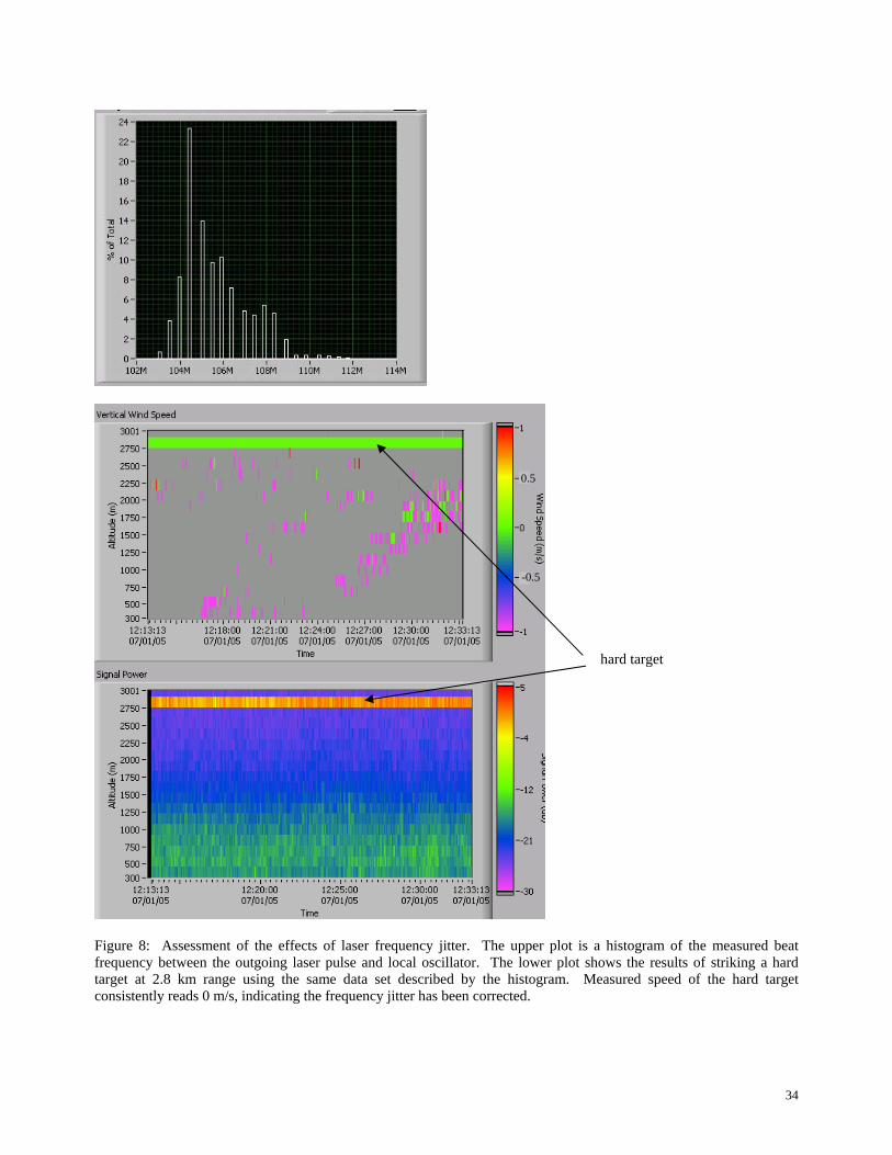
and-fire injection seeding. Figure 8a is a histogram of the frequency offset between the local

oscillator and transmitted pulse for 6000 consecutive pulses. While nominally set for 105 MHz this

14

sample set shows that the actual intermediate frequencies were spread from 103 MHz to 112 MHz.

With the Doppler shift at 2-µm wavelength being 1 MHz per m/s of wind speed, this large range of

frequency jitter must be corrected to obtain accurate wind measurements. The approach for this

correction is to measure the jitter on a pulse-to-pulse basis and compensate for the frequency jitter

before spectral averaging, as described in Section 2.3.

The efficacy of the frequency jitter compensation is tested in the backscatter from the hard

target to verify that the lidar measures the speed at 0 m/s. Figure 8b shows the velocity measured

for the same pulse set of Figure 8a. In this experiment the lidar beam was attenuated to an output

of less than 1 mJ so that the reflection from the hard target was not saturated. The atmospheric

backscatter before the pulse hit the hard target is hence very weak. Though weak, wind

measurements were still made from the aerosol backscatter, but the measurements are mostly out of

the narrow velocity span set in the data display. Such a narrow span was used to resolve any

potential small speed measurements around 0 m/s where the hard target is expected to be. The

velocity from the cell phone tower was indeed found consistently at 0 m/s, at least as processed with

the velocity resolution from the processing parameters used here and described in Section 2.3. The

range measurements to the hard target are also consistent across the measurement set and accurate

to within the processor’s range resolution of 150-m long range bins.

Further system testing was made by making a side-by-side comparison of VALIDAR with a

low-energy commercial Doppler lidar.25 Statistical comparison of the parallel line-of-sight

measurements showed a root-mean-square difference in wind speed measurements of 0.42 m/s.

3. ATMOSPHERIC MEASUREMENTS

15

3.1 Vertical Wind Profiling

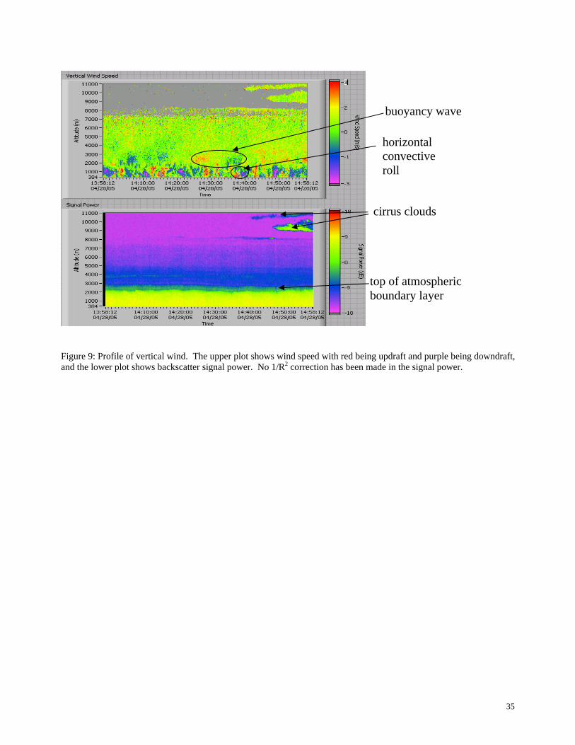
Profiles of the vertical component of wind are shown in Figures 9 and 10. In these data sets

the lidar is pointed toward zenith and wind data is continuously sampled over many minutes with 20

pulses grouped together for averaging and processing. Hence, a vertical wind profile is made every

4 s, resulting in 900 wind profiles in Figure 9 and 300 wind profiles in Figure 10. The upper plot in

each figure is the wind speed versus altitude and the lower plot is signal power versus altitude.

Ordinarily the vertical component of wind is featureless, typically showing speed at or near 0 m/s.

The cases of Figures 9 and 10 are unusual in that strong vertical motions occur. Figure 9 was

recorded over one hour on the gusty afternoon of April 28, 2005. The signal power shows a

typically strong return from the aerosol-rich atmospheric boundary layer (ABL) up to an altitude of

approximately 2 km. Above the ABL the aerosol backscatter drops by more than an order of

magnitude (a backscatter difference as large as two orders of magnitude between the ABL and free

troposphere has been observed in other data). Aerosol backscatter extends to 7.5 to 8.5 km altitude

before the signal drops into noise. The maximum altitude of operation with aerosol backscatter is

highly variable, with season of the year being a strong factor. Over intermittent operations located

at Hampton, Virginia dating back to April 2003 (though with of varying laser pulse energy and lidar

designs as development progressed) the minimum altitude of operation was found to occur in late

Fall and the maximum altitude was found in late Spring. The lowest and highest maximum

altitudes observed were 2 km and 11.5 km, respectively. This qualitative analysis pertains to

aerosol backscatter only; clouds may limit range at low altitudes or provide for higher altitude

operation from cirrus.

16

The vertical wind plot shows turbulent motion within the atmospheric boundary layer, but

near-zero speed in the free troposphere. Some of the turbulent structure in the boundary layer is

seen to be organized in what are perhaps horizontal convective rolls. The wind speed shows

updrafts and downdrafts, both peaking at 3 m/s, as the roll advects across the view of the lidar.

Above these horizontal rolls a series of buoyancy waves were observed with peak speeds of 2 m/s.

A similar measurement scenario has been used to characterize thermals in which birds were

observed to be soaring.26

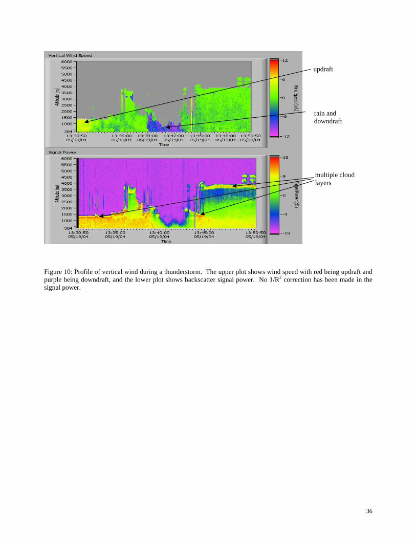
Another interesting example of vertical wind structure is shown in Figure 10, taken during a

thunderstorm. Various cloud layers are seen in this data, with the early phase of the storm

dominated by a low, dense cloud at 1300 m altitude. Under this cloud a sustained updraft reaching

6 m/s occurs as the storm is building up. This updraft subsided and was followed by the low cloud

layer breaking up. Rain is seen near the middle of the data set, marked by speeds reaching 12 m/s.

This downward speed is believed to be the fall of the rain by gravity enhanced by downdraft

pushing the rain drops. Liquid water is effective at absorbing the lidar’s energy, and the signal

power plot shows a variation in the maximum range as the rate of precipitation varies. Water was

also pooling on the output window of the scanner, and the anomaly at 13:44 results from

intentionally spinning the scanner to remove the pooled water. The intense rain from this storm

quickly dissipated to a relatively calm atmosphere, as seen in the lack of turbulence in the wind

speed after 13:45.

3.2 Horizontal and Vertical Wind Profiling

17

A horizontal wind profile can be measured by viewing two orthogonal azimuths at the same

elevation, determining speed along each azimuth, and vector summing the components as a function

of altitude. In this approach the vertical wind component is assumed to be zero. The data

acquisition and control software, described in Section 2, automates steering of the scanner and

collection of data. A typical measurement scenario is to view three different angles with 20 pulses

averaged at each angle. In the following data the horizontal wind field was measured with the beam

oriented at 45 degree elevation (Section 3.2.1 and 3.2.3) or 3 degree elevation (Section 3.2.2) at

azimuths facing north and east, the third angle used is set toward zenith for the vertical wind record.

Scanner angles are calibrated to true compass directions by steering the lidar beam onto a hard

target at a location known in relation to the scanner output by GPS survey. At 5 Hz pulse repetition

rate such a three-direction measurement set requires 25-35 seconds to complete depending on the

extent of data archiving selected. This measurement set, which provides horizontal and vertical

wind profiles, can then be automatically repeated.

3.2.1 High Altitude Wind Profiling

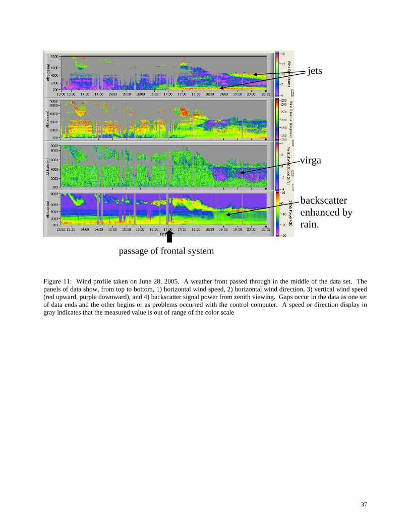
A sample of such a measurement is shown in Figure 11 recorded on June 28, 2005 over a

span of 7 ½ hours, with a frontal system passing through in the middle of the data set. The

horizontal wind speed within the boundary layer significantly increased with the passage of the

front, with the speed peaking in a jet formation of 16 m/s. A higher altitude jet is also seen forming

in the later part of the data. Before passage of the front the horizontal wind speed shows a

transition at 4400 m altitude, above which the speed increased by 3-5 m/s. By referring to the

18

zenith-viewing signal power measurement in the lowest plot this transition at 4400 m altitude also

corresponds to a change in aerosol density.

The wind direction before the front passage shows a shift in direction between the

atmospheric boundary layer and free troposphere, a commonly observed phenomenon, shifting in

this case from southerly to south-westerly flow at higher altitudes. The frontal system brings a

reversal of this relationship of south-westerly flow in the boundary layer and southerly flow in the

free troposphere.

The lower two plots are the wind speed and backscatter power from the third scanner position

of the lidar beam looking toward zenith. The signal power shows clouds below 1000 m and above

6500 m before the front. The low cloud layer lifted with the front. Near 18:30 rain developed,

showing up as enhanced backscatter and also appearing in the velocity measurement as downward

motion reaching 4 m/s. An interesting feature of the rain is that the downward motion ceases at an

altitude near the transition from the atmospheric boundary layer and the free troposphere,

suggesting that the rain evaporates. The lack of rain observed at ground level also indicates that the

precipitation was in the form of virga.

In a separate study, a new algorithm has been applied to the data of Figure 11 that improves

the performance of wind measurements in weak SNR conditions.24 This refined algorithm was run,

however, in post processing as opposed to the real-time results shown in Figure 11.

3.2.2 Low Altitude Wind Profiling

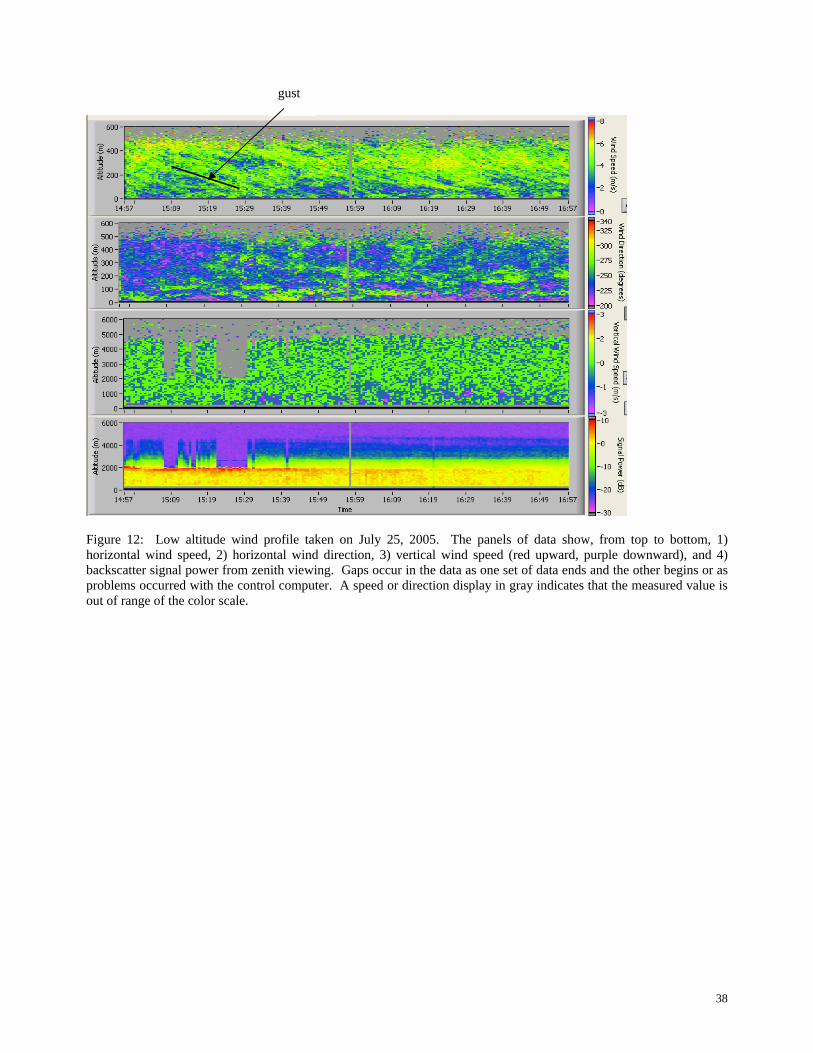
In order to probe the lower atmosphere with higher spatial resolution the elevation angle of

the scanner can be decreased. For example, Figure 12 shows a wind profile taken with an elevation

19

angle of 3 degrees elevation to compose the horizontal wind. The vertical measurements are on a

different scale, and since the lidar is blind for the first 300 m of range the horizontal and vertical

wind measurements do not correspond well in altitude. That is, the low elevation angle for the

horizontal wind measurements is set to probe the lower atmosphere while the zenith-looking

vertical measurement is suited to higher altitudes. The trigonometry of the horizontal measurement

must also be kept in mind when interpreting the wind data, in that the horizontal distance from the

lidar at which the measurements at altitude are made can be large. For example, the horizontal

distance from the lidar at which the 500-m altitude measurement is made is 9.5 km.

An interesting observation of this low attitude measurement example is the movement of

gusts, which can be seen as slanted features in the wind speed measurements of Figure 12. An

ambient wind of 1-3 m/s exists with the occurrence of gusts of 4.5 m/s. The wind speed

measurements show that the 4.5 m/s gusts are first detected at higher altitudes then lower altitudes.

This phenomenon is attributed to the low elevation angle of the lidar beam. That is, if a gust

uniform with altitude approached the lidar it would appear first at high altitudes and slide to lower

altitudes. By this reasoning the speed of the gust could also be calculated by translating altitude to

horizontal distance and noting the time over which the altitude dropped. But making such a

calculation using the slope of the features in Figure 12 results in a gust speed of 3.2 m/s, slower than

the speed extracted directly from Doppler shift. This indirect slope-based calculation, though,

assumes that the gust is a uniform vertically standing plane when it may actually be sloped, an eddy,

or of disorganized spatial structure. This configuration of lidar scan demonstrates an ability to

provide a warning of oncoming gusts.

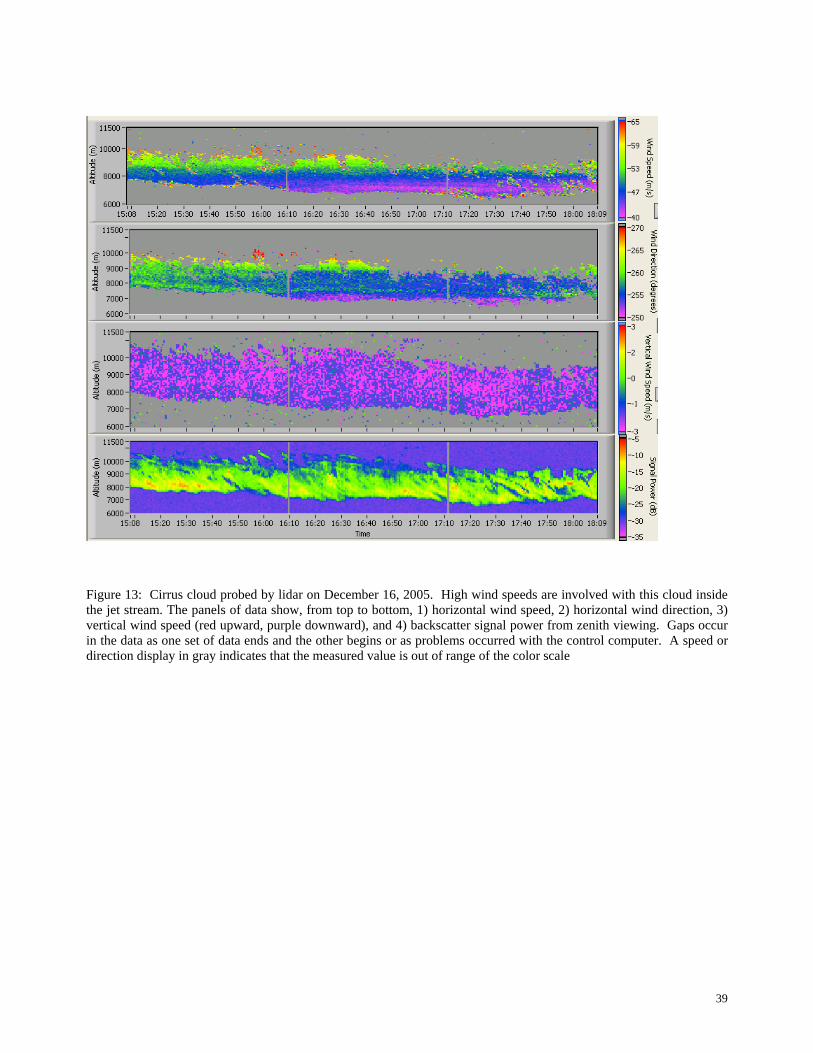
3.2.3 Cirrus Cloud

20

High altitude cirrus clouds have also been characterized with the lidar as shown in Figure 13.

The cloud was observed on December 16, 2005, a time of year when jet stream winds can occur

over the geographical area in which the lidar is located (Hampton, Virginia). A continuum of wind

speeds occurred in altitudes from 7 km to 10 km ranging from 40 m/s to 65 m/s, and showing the

highest known wind speed to be measured with a coherent Doppler lidar. A similarly continuous

variation was found in the wind direction varying through 20 degrees. The zenith viewing

measurements show a downward motion within the cloud, presumably ice crystal virga, ranging

from 1 m/s to 3 m/s with lower speeds more prevalent at the bottom of the cloud. The cloud

descended in height over the 3-hour data set, and the backscatter measurement reveals the cloud to

be dissipating.

4. CONCLUSION

A lidar has been developed from a new type of laser material (Ho:Tm:LuLiF), capable of

generating high-energy 2-µm wavelength pulses for wind and aerosol measurements. Atmospheric

testing has shown the ability to measure wind to higher altitudes than the lower-energy mm lasers

now in use. The system design is scalable to a future space-based instrument, and the atmospheric

tests of the lidar described here were used to predict performance of a space-based lidar.27 More

pulse energy that the 100-mJ class instrument described here can be achieved by adding

amplification stages to the output of the pulsed laser oscillator, an approach that has been taken to

demonstrate an output energy of 1-J per pulse. Moving toward a spaceborne instrument also

21

requires hardening the lidar design for vibration, autonomy, and extreme environments. Work is

currently underway toward a ruggedized version capable of operation from an aircraft. The

atmospheric wind measurements described have proved this testbed to be a valuable tool, as a

ground-based instrument, for performing atmospheric research.

The receiver design is similar to that of Doppler lidars used in previous research, but with the

addition of a dual-balanced photodetector that improves the efficiency of both the receiver and the

use of local oscillator power. A data processing system has been built capable of real-time

reduction of the heterodyne signal to wind and signal backscatter power measurements to ranges of

15 km.

ACKNOWLEGEMENTS

This work was supported by the NASA Laser Risk Reduction Program and the Integrated Program

Office.

REFERENCES

1. S.M. Hannon, S.W. Henderson, J.A. Thomson, and P. Gatt, “Autonomous lidar wind field

sensor: performance predictions,” SPIE Volume 2832, pp. 76-91 (1996).

22

2. C.J. Grund, R.M. Banta, J.L. George, J.N. Howell, M.J. Post, R.A. Richter, A.M.

Weickmann, “High-Resolution Doppler Lidar for Boundary Layer and Cloud Research,” J.

Atmos. And Ocean. Tech, 18, 376-393 (2001).

3. P. Brockman, B.C. Barker, G.J. Koch, D.P.C. Nguyen, and C.L. Britt, “Coherent pulsed

lidar sensing of wake vortex position and strength, winds and turbulence in airport terminal

areas,” Tenth Biennial Coherent Laser Radar Technologies and Applications Conference,

pp. 12-15 (1999).

4. J.G. Hawley, R. Targ, S.W. Henderson, C.P. Hale, M.J. Kavaya, and D. Moerder, “Coherent

launch-site atmospheric wind sounder: theory and experiment,” Appl. Opt. 32, 4557-4568

(1993).

5. R.T. Menzies and R.M. Hardesty, “Coherent Doppler lidar for measurement of wind fields,”

Proc. IEEE 77, 449-462 (1989).

6. M.J. Post and R.E. Cupp, “Optimizing a pulsed Doppler lidar,” Appl. Opt. 29, 4145-4158

(1990).

7. Ch. Werner, P.H. Flamant, O. Reitebuch, F. Kopp, J. Streicher, S. Rahm, E. Nagel, M. Klier,

H. Herrmann, C. Loth, P. Delville, Ph. Drobinski, B. Romand, Ch. Boitel, D. Oh, J. Lopez,

M. Meissonier, D. Bruneau, and A. Dabas, “Wind infrared Doppler lidar instrument,” Opt.

Eng. 40, 115-125 (2001).

8. J. Yu, B.C. Trieu, E.A. Modlin, U.N. Singh, M.J. Kavaya, S. Chen, Y. Bai, P.J. Petzar, and

M. Petros, “1 J/pulse Q-switched 2 µm solid state laser,” Opt. Lett. 31 462-464 (2006).

9. W. Baker, G.D. Emmitt, F. Robertson, R. Atlas, J. Molinari, D. Bowdle, J. Paergle, R.M.

Hardesty, R. Menzies, T. Krishnamurti, R. Brown, M.J. Post, J. Anderson, A. Lorenc, and J.

23

McElroy, “Lidar-Measured Winds from Space: A Key Component for Weather and Climate

Prediction,” Bull. Amer. Meteor. Soc. 76, 869-888 (1995).

10. R.J. Fleming, “National environmental observing system to mitigate the effects of a nuclear-

biological-chemical (NBC) attacks: strategic and tactical,” SPIE Volume 5071, pp. 22-32

(2003).

11. American National Standard Z136.6-2005, “Safe use of lasers outdoors.”

12. S.W. Henderson, C.P. Hale, J.R. Magee, M.J. Kavaya, and A.V. Huffaker, “Eye-safe

coherent laser radar system at 2.1 µm using Tm,Ho:YAG lasers,” Opt. Lett. 16, 773-775

(1991).

13. B.M. Walsh, N.P. Barnes, M. Petros, J. Yu, and U.N. Singh, “Spectroscopy and modeling of

solid state lanthanide lasers: Application to trivalent Tm3+ and Ho3+ in YLiF4 and LuLiF4,”

J. Appl. Phys. 95, 3255-3271 (2004).

14. M. Petros, J. Yu, T. Melak, B. Trieu, S. Chen, U. Singh, and Y. Bai, “High energy totally

conductive cooled, diode pumped, 2 µm laser,” Advanced Solid-State Photonics

Conference, OSA Trends in Optics and Photonics Volume ? , 2005.

15. C. Hale, S.W. Henderson, and D.M. D’Epagnier, “Tunable Highly-Stable Maser/Local

Oscillator Lasers for Coherent Lidar Applications,” in Proceedings of the Tenth Biennial

Coherent Laser Radar Technology and Applications Conference, 115-118, 1999.

16. S.W. Henderson, E.Y. Yuen, and E.S. Fry, “Fast resonance detection technique for single-

frequency operation of injection seeded Nd:YAG lasers,” Opt. Lett. 11, 715-717 (1986).

17. USF HITRAN-PC, Version 2.51 (Ontar Corporation, North Andover, Mass., 1996)

24

18. G.J. Koch, B.W. Barnes, M. Petros, J.Y. Beyon, F. Amzajerdian, J. Yu, R.E. Davis, S.

Ismail, S. Vay, M.J. Kavaya, and U.N. Singh, “Coherent Differential Absorption Lidar

Measurement of CO2,” Appl. Opt. 43, 5092-5099 (2004).

19. M. Cvijetic, “Coherent and Nonlinear Lightwave Communications,” Artech house, Inc.,

Norwood, MA (1996).

20. F. Amzajerdian, “Analysis of Optimum Heterodyne Receivers for Coherent Lidar

Applications,” Proc. of 21th International Laser Radar Conference, Quebec, Canada, July 8-

12, 2002.

21. J.Y. Beyon and G.J. Koch, “Resolution study of wind parameter estimates by a coherent

Doppler lidar system,” Proc. of SPIE Vol.6214, 621403 (2006).

22. J.Y. Beyon, G.J. Koch, and Z. Li, “Noise normalization and windowing functions for

VALIDAR in wind parameter estimation,” Proc. of SPIE Vol.6214, 621404 (2006).

23. J.Y. Beyon and G.J. Koch, “Wind profiling by a coherent Doppler lidar system VALIDAR

with a subspace decomposition approach,” Proc. of SPIE Vol.6236, 623605-1 (2006).

24. J. Y. Beyon and G. J. Koch, “Novel Nonlinear Adaptive Doppler Shift Estimation

Technique for the Coherent Doppler Validation Lidar” Opt. Eng. accepted for publication,

August 2006.

25. G.D. Emmitt, S.A. Wood, and G.J. Koch, “Comparison of VALIDAR and GWOLF Doppler

Lidar Measurements,” 2nd Symposium on Lidar Atmospheric Applications, American

Meteorological Society 85th Annual Meeting, 2005.

26. G.J. Koch, “Using a Doppler light detection and ranging (lidar) system to characterize an

atmospheric thermal providing lift for Soaring Raptors,” J. Field Ornithol. 77 (2006),

25

27. M.J. Kavaya, G.J. Koch, F. Amzajerdian, B.W. Barnes, R.E. Davis, U.N. Singh, R.G.

Frehlich, “Estimating Space Performance of a Coherent Doppler Wind Lidar by Inverting

Ground Performance,” Working Group on Space-Based Lidar Winds, Welches, OR, July

2005.

28. A.E. Siegman, “Defining, measuring, and optimizing laser beam quality,” Proc. SPIE 1868

(1993).

26

Laser material: Ho:Tm:LuLiF Pulse energy: 90 mJ operationally, capable of 100 mJ Pulse width: 140 ns Pulse repetition rate: 5 Hz, 10 Hz at reduced energy Spectrum: single frequency Wavelength: 2053.5 nm Wavelength tuning: 3-4 nm including CO2 lines Beam quality (M2): < 1.2 times diffraction limit28 Detector: InGaAs in dual-balanced configuration Telescope aperture: 6 inches Scanner: 8.5 inch aperture full hemispherical coverage Table 1: Specifications of VALIDAR

27

90/10 coupler

cw masteroscillator laser

pulsed laserPBS

telescope? /4

dual -balancedInGaAsphotodiodes

90/10 coupler

cw masteroscillator laser

pulsed laserPBS

telescope? /4

dual -balancedInGaAsphotodiodes

50/50 Coupler

acousto -opticmodulator

isolator

isolatorisolator

Q -switch

Ho:Tm:YLFPZT

? /2

? /2

? /2telescope

λ /4

dual -balancedInGaAsphotodiodes

50/50 Coupler

Outgoing Pulse

Atmospheric Return

Local Oscillator

Heterodyne pulse monitoracousto -opticmodulator

isolator

isolator isolator

Q-switchHo:Tm:LuLiFPZT

resonancedetectorresonancedetector

λ /2

λ /2

λ /2pulsemonitor

90/10 coupler

Figure 1: Optical layout of VALIDAR. Fiber optic paths are indicated by a circular bend in the path.

28

Figure 2: Exploded view of laser head assembly.

laser rod

flow tube

diode heat sinks

diode laser arrays

29

Figure 3: Signal involved with ramp-and-fire injection seeding technique. The lower curve is a monitor of the ramp voltage applied to the piezo-electric translator (PZT) to change the pulsed laser cavity length. The upper plot shows the CW injection seed in resonance with the pulsed laser cavity. An electronic circuit fires the Q-switch when a resonance is detected.

30

Figure 4: Injection seeding results in a single frequency spectrum as monitored by a photodiode outside the laser cavity. The temporal profile (channel 1) of the pulse shows a pulse width of 142 ns and a smooth gaussian shape. Without injection seeding this gaussian envelope would be modulated by mode beating between longitudinal modes of the laser cavity. Channel 2 and its discrete Fourier transform (middle plot) show the heterodyne signal of the laser pulse—this signal is used by the signal processing system to determine pulse-to-pulse frequency jitter.

31

Figure 5: Diagram of the dual-balanced heterodyne detector. The polarity of the photodiodes allows cancellation of AM noise that might be present on the local oscillator. Fiber optic pigtails are attached to the photodiodes.

Detector # 1

Detector # 2

RB

VB

Amplifiers

RB

- VB

OutputSignal

Detector # 1

Detector # 2

RB

VB

Amplifiers

RB

- VB

OutputSignal

32

Figure 6: Layout of the VALIDAR electronics and signal processing system.

Outgoing Pulse

Lidar Return

RS-232

CompactPCI Bus

Data Acquisition and Processing System

CompactPCI Chassis

Scanner Control Computer

Lidar Transceiver

Real-Time Display & User Interface

Analog Front End Digitizer

Digital Signal Processor--2 cards of 4 chips

Control Program

Host CPU

Storage Devices

33

Figure 7: Backscatter (lower plot) from a single pulse. Two heterodyne detectors are used to compose this signal with a switch selecting the two channels—the transient from this electronic switch can by seen at approximately 1.2 µs from the trigger. Before the switch is the pulse monitor from which the zero frequency for Doppler processing is determined. The second channel is taken from the dual-balanced detector for the atmospheric backscatter. 1/R2 decay in the signal strength can be seen in the envelope of the backscatter.

trigger

aerosol scatter

scatter from optics (het. monitor pulse)

34

Figure 8: Assessment of the effects of laser frequency jitter. The upper plot is a histogram of the measured beat frequency between the outgoing laser pulse and local oscillator. The lower plot shows the results of striking a hard target at 2.8 km range using the same data set described by the histogram. Measured speed of the hard target consistently reads 0 m/s, indicating the frequency jitter has been corrected.

0.5

-0.5

hard target

35

Figure 9: Profile of vertical wind. The upper plot shows wind speed with red being updraft and purple being downdraft, and the lower plot shows backscatter signal power. No 1/R2 correction has been made in the signal power.

buoyancy wave

horizontal convective roll

cirrus clouds

top of atmospheric boundary layer

36

Figure 10: Profile of vertical wind during a thunderstorm. The upper plot shows wind speed with red being updraft and purple being downdraft, and the lower plot shows backscatter signal power. No 1/R2 correction has been made in the signal power.

updraft

rain and downdraft

multiple cloud layers

37

Figure 11: Wind profile taken on June 28, 2005. A weather front passed through in the middle of the data set. The panels of data show, from top to bottom, 1) horizontal wind speed, 2) horizontal wind direction, 3) vertical wind speed (red upward, purple downward), and 4) backscatter signal power from zenith viewing. Gaps occur in the data as one set of data ends and the other begins or as problems occurred with the control computer. A speed or direction display in gray indicates that the measured value is out of range of the color scale

passage of frontal system

jets

virga

backscatter enhanced by rain.

38

Figure 12: Low altitude wind profile taken on July 25, 2005. The panels of data show, from top to bottom, 1) horizontal wind speed, 2) horizontal wind direction, 3) vertical wind speed (red upward, purple downward), and 4) backscatter signal power from zenith viewing. Gaps occur in the data as one set of data ends and the other begins or as problems occurred with the control computer. A speed or direction display in gray indicates that the measured value is out of range of the color scale.

gust

39

Figure 13: Cirrus cloud probed by lidar on December 16, 2005. High wind speeds are involved with this cloud inside the jet stream. The panels of data show, from top to bottom, 1) horizontal wind speed, 2) horizontal wind direction, 3) vertical wind speed (red upward, purple downward), and 4) backscatter signal power from zenith viewing. Gaps occur in the data as one set of data ends and the other begins or as problems occurred with the control computer. A speed or direction display in gray indicates that the measured value is out of range of the color scale