High Efficiency Video Coding (HEVC)

Oscar C. Au (PhD, Princeton Univ)

Dept of Electronic and Computer EngineeringHong Kong University of Science and Technology

Email: eeau@ust.hk

Oscar C. Au

• BS,Toronto.MA/PhD,Princeton.Postdoc,Princeton.• Professor,HKUST.Director,MultimediaTechCenter.• SteeringCommittee,ICME/TMM.• IEEE/HKIEFellow.BoG,APSIPA.• BestPaperAwards:SiPS/PCM/MMSP/ICIP• AE of8journals:TCSVT,TIP,TCAS1,TVCIR,JSPS,TSIP,JMM,JFI.• Chairof3TC:CASMSATC,SPSMMSPTC,APSIPAIVMTC.• Memberof5TC:CASVSPS/DSP,SPSIVMSP/IFS,ComSoc MMC.• 400+papers.H‐index=29.100+patentsfiled.20granted.• 80+standardcontribution(MPEG/VCEG/JCTVC/AVS).

Outline

HEVC standardization status HEVC structure Intra Prediction Inter Prediction Scanning/ Transform Entropy coding In-loop filtering Parallel processing Performance Continuing Work

Development of Video Coding Standards

H.261(1990)

MPEG-1(1993)

H.263(1996)

H.263+(1998)

H.263++(2000)

H.264(AVC)(2004)

MPEG-4 v1(1999)

MPEG-4 v2(2000)

MPEG-4 v3(2001)

1990 1992 1994 1996 1998 2000 2002 2004 2006 2008 2010 20121990 1992 1994 1996 1998 2000 2002 2004 2006 2008 2010 2012

MPEG-2(H.262)(1995)

ISO/IECMPEG

ITU-TVCEG

SVC(H.264-G)(2007)

HEVC(H.265)(2013)

5

High Efficiency Video Coding (HEVC)

• A new standard under development by ISO andITU-T

– Joint MPEG & VCEG new team: JCT-VC

• Target at HDTV or ultra-HDTV compression, withsubstantially improved coding efficiency comparedto H.264/AVC, i.e. 50% bit rate reduction

• Very active project (hundreds of documents everymeeting), very diverse company & universityparticipation.

5

6

HEVC Timeline

2010.01 Formal joint CfP from VCEG and MPEG

2010.04 JCT-VC team, HEVC joint project, full proposals

2010.07 TMuC SW ready, tool experiments (TE)

2010.10 HM SW ready, core experiments (CE)

2011.02 WD

2012.02 CD

2012.07 DIS

2012.10 SoDIS (Study of Draft International Standard)

HEVC conformance testing is triggered.

2013.01 FDIS (expected)

HEVC Meetings

7

Location Attendees Documents1 Dresden 188 ~402 Geneval 221 ~1203 Guangzhou 244 ~3004 Daegu 248 ~4005 Geneva 226 ~5006 Torino 254 ~7007 Geneva 284 ~10008 San Jose 255 ~7009 Geneva 2xx ~55010 Stockholm 2xx ~50011 Shanghai 235 ~350

Typical HEVC video coding structure

8

HEVC Architecture

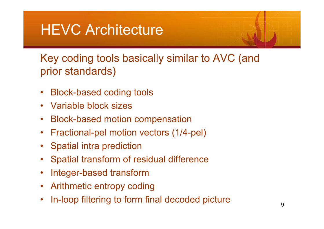
Key coding tools basically similar to AVC (and prior standards)

• Block-based coding tools• Variable block sizes• Block-based motion compensation• Fractional-pel motion vectors (1/4-pel)• Spatial intra prediction• Spatial transform of residual difference• Integer-based transform• Arithmetic entropy coding • In-loop filtering to form final decoded picture

9

Picture Coding structure

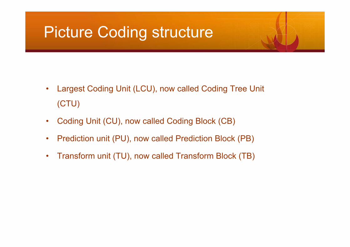
• Largest Coding Unit (LCU), now called Coding Tree Unit

(CTU)

• Coding Unit (CU), now called Coding Block (CB)

• Prediction unit (PU), now called Prediction Block (PB)

• Transform unit (TU), now called Transform Block (TB)

Picture Coding structure

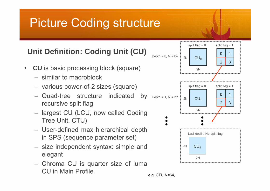
• CU is basic processing block (square)– similar to macroblock– various power-of-2 sizes (square)– Quad-tree structure indicated by

recursive split flag– largest CU (LCU, now called Coding

Tree Unit, CTU)– User-defined max hierarchical depth

in SPS (sequence parameter set)– size independent syntax: simple and

elegant– Chroma CU is quarter size of luma

CU in Main Profilee.g. CTU N=64,

Unit Definition: Coding Unit (CU)

Picture Coding structure

0/1 shows the quad-tree splitting flag

LCU Quad-tree split example

Picture Coding Structure

• Prediction Unit (PU) is the basic unit for prediction

Example: Available PU for 64x64 CU– Skip: PU = 64x64– Intra: PU = 64x64– Inter: PU = 64x64, 64x32, 32x64, (32x32)

64x16, 64x48, 16x64, 48x64

Example: Available PU for 64x64 CU– Skip: PU = 64x64– Intra: PU = 64x64– Inter: PU = 64x64, 64x32, 32x64, (32x32)

64x16, 64x48, 16x64, 48x64

– PU is the basic unit for prediction of a 2Nx2N CU• 2Nx2N, NxN, 2NxN, Nx2N, 2NxnU, 2NxnD, nLx2N, nRx2N

– Allowed PU partitions are depending on prediction type• NxN PU allowed only for minimum CU. NOT allowed for larger CU.• Asymmetric motion partition or AMP (2NxnU, 2NxnD, nLx2N, nRx2N) is not

applied to inter 8x8 CU. (i.e. 2x8, 6x8, 8x2, 8x6 not allowed)

Picture Coding Structure

• Transform Unit (TU) is basic unit for transform andquantization.

– Each CU subdivided into square TU using quad-tree (split flag)– One square transform for each TU (DCT for inter/intra, DST for 4x4 intra

luma)

Solid line=CU, dashed gray line=TU

Picture Coding Structure

• Transform Unit (TU) is the basic unit for transform andquantization.

• For inter, may exceed size of PU, but cannot exceed size of CU • For intra, cannot exceed PU size • MaxTUSize is coded in SPS, its value in range of [4, 8, 16, 32]• In HM, Max. TU size is 32x32 for Luma and 16x16 for Chroma • Absolute Min. TU size is 4x4 for both Luma and Chroma

– MaxTUDepth is coded in SPS to control the minTUSize.– Separate MaxTUDepth control for intra and inter.

Picture Coding Structure

• An example of the CU, PU & TU in a LCU

• MaxTUDepth = 3 in this example

• Flags to indicate the TU split status

• Max TU is 32x32 for Luma and 16x16 for chroma

• Min TU is 4x4 for luma & chroma

• The green TU block is not applicable to intra_NxN PUs

Intra Prediction

• Intra PCM mode

• Intra Luma and Chroma prediction modes

• Intra reference padding

• Mode dependent intra reference sample filtering

17

Intra Prediction

• Intra PCM mode– In I_PCM mode, prediction, transform, quantization and entropy

coding are bypassed.

– Samples are directly represented by a predefined number of bits. (signal characteristic are ill-posed, e.g. noise-like signals.)

– I_PCM mode is only available for 2Nx2N PU• Max and min I_PCM CU size is signalled in SPS• Legal I_PCM CU sizes are 8x8, 16x16 and 32x32• User-selected PCM sample bit-depths, signalled in SPS for

luma and chroma, separately

– Take Luma sample as an example:

recSamplesL[ i, j ] = pcm_sample_luma[ ( nS * j ) + i ] << ( BitDepthY – PCMBitDepthY )

• Lossless coding when PCMBitDepthY=BitDepthY.

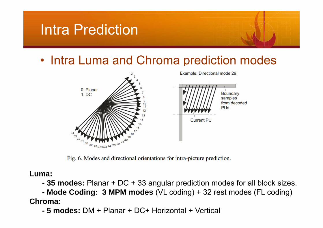
Intra Prediction

• Intra Luma and Chroma prediction modes

Luma:- 35 modes: Planar + DC + 33 angular prediction modes for all block sizes.- Mode Coding: 3 MPM modes (VL coding) + 32 rest modes (FL coding)

Chroma: - 5 modes: DM + Planar + DC+ Horizontal + Vertical

Intra Prediction

• Planar mode (Surface fitting)• Final T at (0, N+1), final L at (N+1, 0)

+ >> 1

T

L

T

T

L L

Interpolation indicated by dashed arrow Replication indicated by dotted arrow

Intra Prediction

• DC mode

• A variable DCVal is derived as (k=log2(nS))

predSamples[ x, y ] = DCVal, with x, y = 0..nS-1

• Boundary smoothing is applied on Luma DC predictions when TU size is less than 32x32

• predSamples[ 0, 0 ] = (p[ -1, 0 ] + 2*DCVal + p[ 0, -1 ] + 2 ) >> 2• predSamples[ x, 0 ] = (p[ x, -1 ] + 3*DCVal + 2 ) >> 2, with x = 1..nS-1 • predSamples[ 0, y ] = (p[ -1, y ] + 3*DCVal + 2 ) >> 2, with y = 1..nS-1

)1(]',1[]1,'[1

0'

1

0'

knSypxpnS

y

nS

x

Intra Prediction

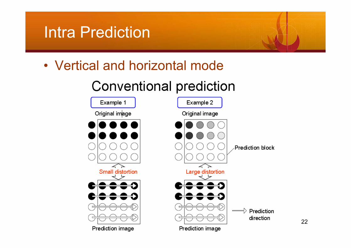
• Vertical and horizontal mode

22

Intra Prediction

• Vertical and horizontal mode

Intra Prediction

• Intra Reference Padding

• Totally nS*4+1 ref. samples from top & left neighbours for a nS*nSTU

p[x,y] with x = -1, y = -1..nS*2-1 and x = 0..nS*2-1, y = -1

• p[x,y] is marked “unavailable” when:

- the corresponding neighbour TU is not available,

- it is not intra coded & constrained_intra_pred_flag = 1

Intra Prediction

• Mode dependent intra reference sample filtering

Filtering ref. samples before using them to predict current TUOnly applied to Luma component, no smoothing for Chroma

Mode dependent filtering condition4x4: No filtering8x8: Only filtering for mode 0, 2, 18, 3416x16: Filter for all modes except 1, 9, 10, 11, 25, 26, 2732x32: Filter for all modes except 1, 10, 26

Smoothing filtering Filter {1 2 1} is applied when filtering is needed No smoothing for the right-most and bottom-most ref. pixels L-shape {1 2 1} filter for the corner ref. pixel

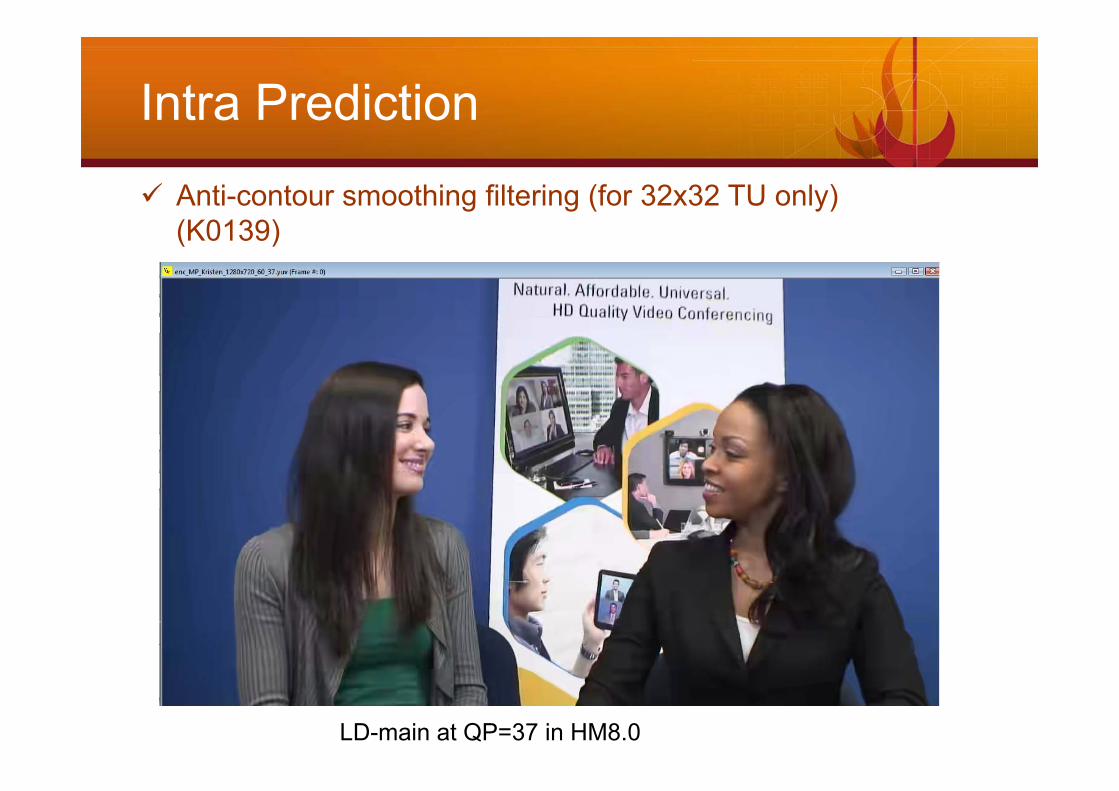
Intra Prediction

Anti-contour smoothing filtering (for 32x32 TU only) (K0139)

LD-main at QP=37 in HM8.0

Intra Prediction

Anti-contour smoothing filtering (for 32x32 TU only) (K0139)

ref[0]

ref[63]

ref[65] ref[128] ref[64]

Direction of intra prediction

Block edge in reconstructed reference is propagated to a non-block boundary location

32x32 Intra predicted

samples

Propagation of discontinuity at block boundary to sample locations within the predicted sample array.

When:- strong_intra_smoothing_enable_fla

g=1- If |p0+p2-2*p1|>T, linear

interpolation between p0 and p2 before intra-prediction

Top-left (p[-1, -1]), right most (p[63, -1]) and bottom most (p[-1, 63]) ref. samples are unchanged

Weighted average for the left and above ref. sample line(Bi-linear)

Inter Prediction

• Limits on small PU sizes• AMVP • Merge• Interpolation filters• Reference motion data compression

28

Inter Prediction

• Limits on small PU size

– Inter_NXN is only allowed for smallest allowed CU size.

– Bi-directional prediction is not allowed for inter 8x4 and 4x8 For AMVP For merge

Inter Prediction

• AMVP• Advanced Motion Vector Prediction (AMVP)

– Two MVP candidates for one reference list– Explicit motion vector predictor signaling

Two reference lists for bi-prediction.

One MVP index for each reference list.

MV difference (MVD) will be coded

Each PU has its own reference index and MVs

Inter Prediction

• AMVP• Construction process of AMVP MVP candidate list

– Two predictors derived from 2 spatial candidates and 1 temporal candidate Spatial A: the first available one of A0 & A1

Spatial B: the first available one of B0, B1 & B2

If A is equal to B, drop B and add the temporal candidate

If list size < 2, add zero motion candidate

Fix final list size to 2Two spatial 

candidate derivationOne temporal 

candidate derivation

Candidate list pruning

Candidate list construction

Fill zero MV if list size < 2

Final 2 motion vector candidates

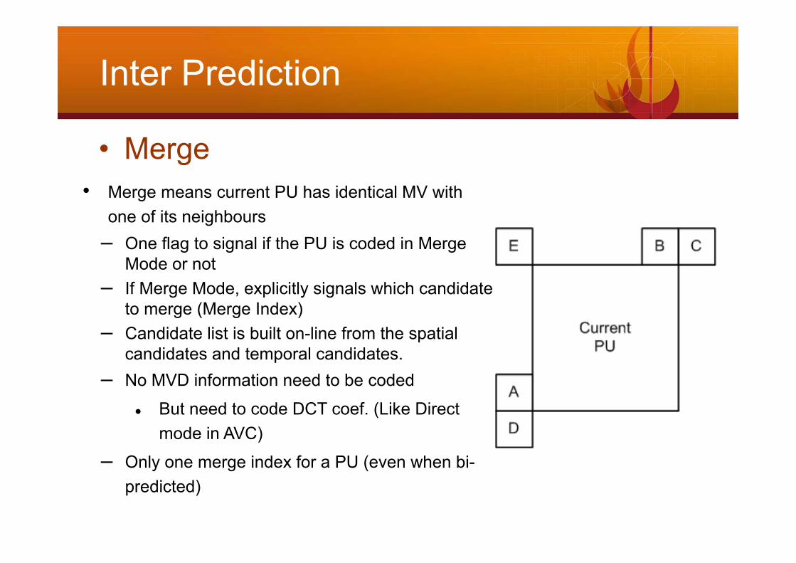
Inter Prediction

• Merge• Merge means current PU has identical MV with

one of its neighbours– One flag to signal if the PU is coded in Merge

Mode or not– If Merge Mode, explicitly signals which candidate

to merge (Merge Index)– Candidate list is built on-line from the spatial

candidates and temporal candidates.– No MVD information need to be coded

But need to code DCT coef. (Like Direct mode in AVC)

– Only one merge index for a PU (even when bi-predicted)

Inter Prediction

• Interpolation filters for lumaA-1,-1 A0,-1 a0,-1 b0,-1 c0,-1 A1,-1

A-1,0 A0,0 A1,0

A-1,1 A0,1 A1,1a0,1 b0,1 c0,1

a0,0 b0,0 c0,0

d0,0

h0,0

n0,0

e0,0

i0,0

p0,0

f0,0

j0,0

q0,0

g0,0

k0,0

r0,0

d-1,0

h-1,0

n-1,0

d1,0

h1,0

n1,0

A2,-1

A2,0

A2,1

d2,0

h2,0

n2,0

A-1,2 A0,2 A1,2a0,2 b0,2 c0,2 A2,2

• For Luma fractional pixels– A single consistent separable

interpolation process to generate all fractional positions .

– Pixel accuracy is 1/4– 7-tap for quarter pixel and 8-tap for

half pixel– Filter kernel were partially derived

from DCT basis function equations.

Inter Prediction

• Interpolation filters for chroma

B0,0 ae0,0 ag0,0 ah0,0ab0,0 ac0,0 ad0,0 af0,0 B1,0

B1,1B0,1

be0,0 bg0,0 bh0,0bb0,0 bc0,0 bd0,0 bf0,0ba0,0

ce0,0 cg0,0 ch0,0cb0,0 cc0,0 cd0,0 cf0,0ca0,0

de0,0 dg0,0 dh0,0db0,0 dc0,0 dd0,0 df0,0da0,0

ee0,0 eg0,0 eh0,0eb0,0 ec0,0 ed0,0 ef0,0ea0,0

fe0,0 fg0,0 fh0,0fb0,0 fc0,0 fd0,0 ff0,0fa0,0

ge0,0 gg0,0 gh0,0gb0,0 gc0,0 gd0,0 gf0,0ga0,0

he0,0 hg0,0 hh0,0hb0,0 hc0,0 hd0,0 hf0,0ha0,0

ah-1,0

bh-1,0

ch-1,0

dh-1,0

eh-1,0

fh-1,0

gh-1,0

hh-1,0

he0,-1 hg0,-1 hh0,-1hb0,-1 hc0,-1 hd0,-1 hf0,-1ha0,-1

ba1,0

ca1,0

da1,0

ea1,0

fa1,0

ga1,0

ha1,0

ae0,1 ag0,1 ah0,1ab0,1 ac0,1 ad0,1 af0,1

• For Chroma fractional pixels– Pixel accuracy is 1/8– ab0,0, ac0,0, ad0,0, ae0,0, af0,0,

ag0,0, ah0,0 : 4-tap filtering on Bi,0 (i = −1..2) in hor. Direction

– ba0,0, ca0,0, da0,0, ea0,0, fa0,0, ga0,0, ha0,0 : 4-tap filtering on B0,j(j = −1..2) in vert. direction

– bX0,0, cX0,0, dX0,0, eX0,0, fX0,0, gX0,0 hX0,0 (X = b, c, d, e, f, g, h) : 4-tap filter aX0,i (i = −1..2) in vert. direction

– Different filter coefficients for different positions.

1/8: {-2, 58, 10, -2} 1/4: {-4, 54, 16, -2}3/8: {-6, 46, 28, -4} 1/2: {-4, 36, 36, -4}

Scanning/ Transform

• Mode dependent coefficient scanning (MDCS)

• Coefficient Grouping (CG)• Intra DCT/DST transforms• Transform skip

35

Scanning/ Transform

• Scanning- No zigzag scan for coefficients scanning in HEVC.

- Inter block uses Diagonal scan

- MDCS applies to only 4x4 and 8x8 TU in intra.

• MDCS Scan pattern is determined based on TU size and intra prediction mode– Diagonal scan, Horizontal scan, Vertical scan– A LUT is defined as shown in next slide

Scanning/ Transform

• Scanning0: Diagonal, 1: Horizontal, 2: Vertical

IntraPredMode log2TrafoSize − 20 (4x4) 1 (8x8) 2 (16x16) 3 (32x32)

0 1 1 0 01 2 2 0 0

2-3 0 0 0 04-5 1 1 0 06 0 0 0 0

7-8 2 2 0 09-10 0 0 0 011-12 1 1 0 013-14 0 0 0 015-16 2 2 0 017-19 0 0 0 020-23 1 1 0 024-27 0 0 0 028-31 2 2 0 032-33 0 0 0 0

34 0 0 0 035 0 0 0 0

Scanning/ Transform

• Coefficient grouping

CG structure of a 16x16 TU

- TU larger than 4x4 will be sub-divided

into CGs of size 4x4, and scanned at 2

levels.

- Significant_coef_CG_flag is signaled for

each CG level to indicate whether the

CG has non-zero coefficients.

Scanning/ Transform

• Transform• Integer DCT/DST transform on scaled coefficients

– DST is applied to intra 4x4 Luma TU, DCT is applied to other TUs– Core transforms: 32x32, 16x16, 8x8, 4x4

• Transform skipping of 4x4 TU– A solution for screen content coding in HEVC

– BD rate reduction on class F: 7.8/5.6/3.4% for AI/RA/LD– This feature could be turn on by transform_skip_enabled_flag in PPS

– Both luma and chroma 4x4 TUs could be transform skipped– If on, a flag per 4x4 TU to indicate transform skip is applied or not

– No change to prediction, CABAC, in-loop filter, coef. scan and quantization

Entropy Coding

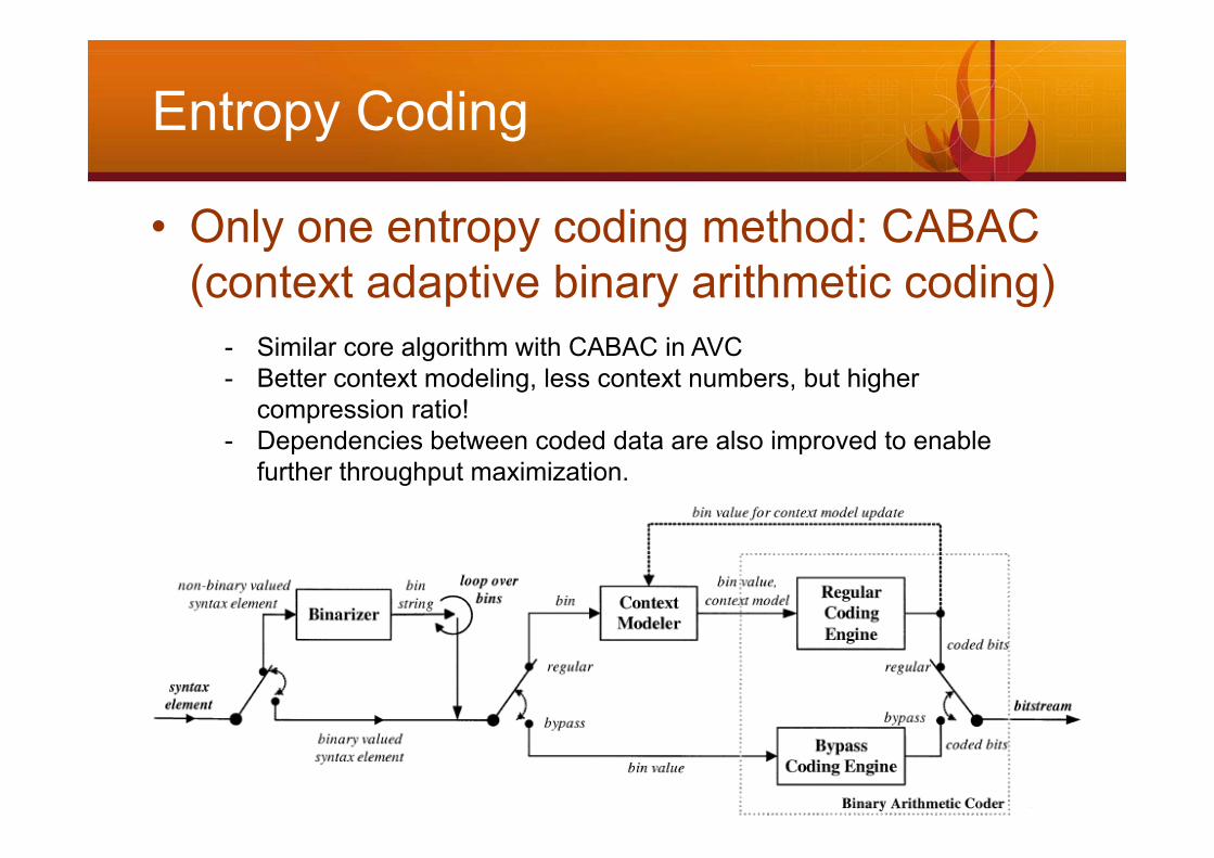
• Only one entropy coding method: CABAC (context adaptive binary arithmetic coding)

- Similar core algorithm with CABAC in AVC- Better context modeling, less context numbers, but higher

compression ratio!- Dependencies between coded data are also improved to enable

further throughput maximization.

In-loop filtering

• Cascaded in-loop filters

Deblocking filter

SampleAdaptive

Offset

• Deblocking filter to reduce blocking artifact– HEVC uses similar (boundary strength based) deblocking filter as

H.264/AVC but Suitable modification for big blocks and complex TU boundaries Filtering order modification for parallel processing

• Sample adaptive offset (SAO) – Adaptively add offsets to enhance deblocked pixels– Each LCU can be enhanced by Band Offset or Edge Offset

In-loop filtering

• Deblocking filter: Block strength (bS) decision • Filtering a picture in LCU unit

• Picture vertical edge filtering first, then picture horizontal edge filtering

• Filtering both PU and TU edges• For both Luma and Chroma• Expect the picture boundary• bS calculated for each 4 pixels along the

PU/TU edges• Chroma shares the same bS with Luma

• Deblocking steps for a LCU• Derive TU and PU edges• Derive bS values• Filter luma edges

• Decision (no-/weak-/strong-filtering)• Filtering

• Filter chroma edges• Filtering

In-loop filtering

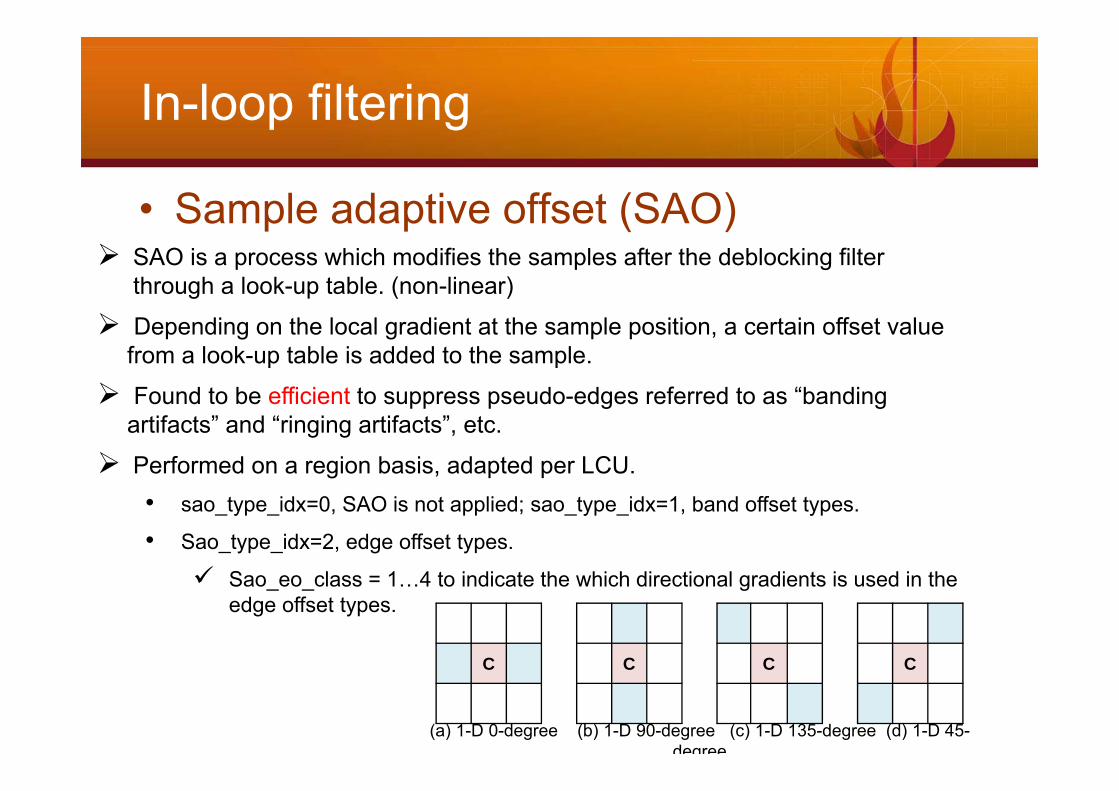
• Sample adaptive offset (SAO) SAO is a process which modifies the samples after the deblocking filter

through a look-up table. (non-linear)

Depending on the local gradient at the sample position, a certain offset value from a look-up table is added to the sample.

Found to be efficient to suppress pseudo-edges referred to as “banding artifacts” and “ringing artifacts”, etc.

Performed on a region basis, adapted per LCU.• sao_type_idx=0, SAO is not applied; sao_type_idx=1, band offset types.

• Sao_type_idx=2, edge offset types.

Sao_eo_class = 1…4 to indicate the which directional gradients is used in the edge offset types.

CCCC

(a) 1-D 0-degree (b) 1-D 90-degree (c) 1-D 135-degree (d) 1-D 45-degree

In-loop filtering

• Sample adaptive offset (SAO)• For a specified EO type, decoder derives for each pixel which category it

belongs to, and then add the received offset of the category to the pixel– 4 offsets are sent to decoder for categories 1~4– Offset value should be >=0 for category 1 & 2, and <= 0 for category 3 & 4.

Category Condition1 c < 2 neighboring pixel values2 c < 1 neighbor && c == 1 neighbor3 c > 1 neighbor && c == 1 neighbor4 c > 2 neighbors0 None of the above

In-loop filtering

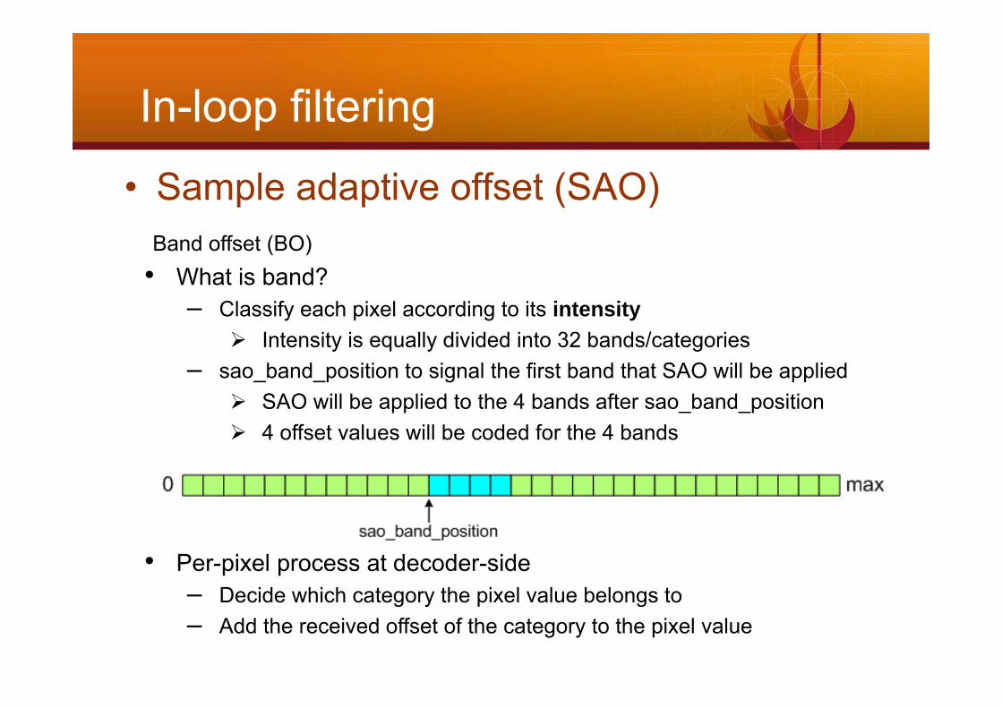
• Sample adaptive offset (SAO)Band offset (BO)

• What is band?– Classify each pixel according to its intensity

Intensity is equally divided into 32 bands/categories– sao_band_position to signal the first band that SAO will be applied

SAO will be applied to the 4 bands after sao_band_position 4 offset values will be coded for the 4 bands

• Per-pixel process at decoder-side– Decide which category the pixel value belongs to– Add the received offset of the category to the pixel value

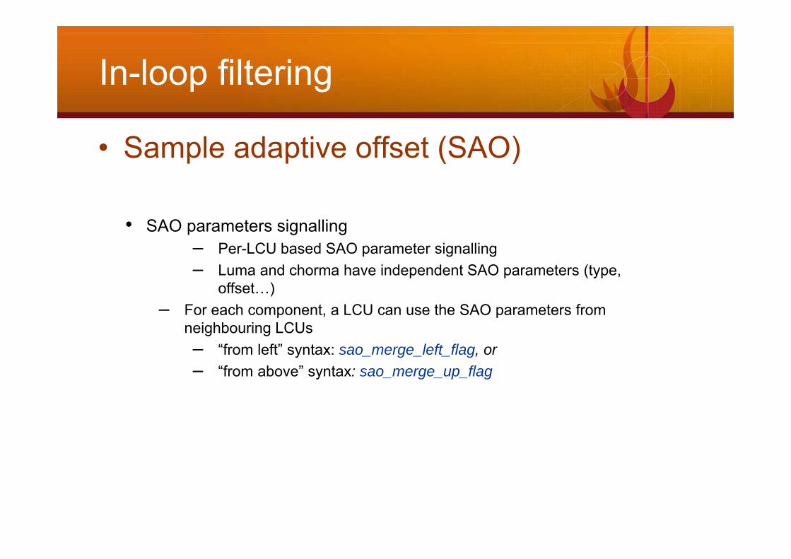
In-loop filtering

• Sample adaptive offset (SAO)

• SAO parameters signalling– Per-LCU based SAO parameter signalling– Luma and chorma have independent SAO parameters (type,

offset…)– For each component, a LCU can use the SAO parameters from

neighbouring LCUs– “from left” syntax: sao_merge_left_flag, or– “from above” syntax: sao_merge_up_flag

Parallel processing

• WPP (Wave-front parallel processing)• Tile base partition

(WPP is not allowed to be used in combination with tiles in HEVC)

47

Parallel processing

• WPP (Wave-front parallel processing)

X

X

X

X

X

KEY

1

2

3

4

5

6

Chunk

CABAC probabilitiesPixel/MV dependencyProbabilities dependencyBlock(s) being encoded

At the end of each LCU line– Perform a CABAC flush of LCU line (write remaining bits + stop bit)– Initialize CABAC states (lower bound L and range R of the interval) – Then, Each line produces a “Chunk” of compressed data

Parallel processing

• Tiles• What is “tile”?

– Self-contained and independently-decodable rectangular regions of the picture.– Vertical and horizontal boundaries partition of a picture into columns and rows– Boundary locations may be specified individually or uniformly spaced (signalled

in SPS and PPS)– Always rectangular with an integer number of LCUs

• Why partitioning into tiles?– High level parallel processing

Parallel processing

• WPP (Wave-front parallel processing)• Tile base partition

50

Performance

• HEVC Draft 7 Main Profile .vs. AVC High Profile (J0236)

All Intra Random Access Low Delay

Class A −23.4% −36.9%Class B −22.8% −39.5% −41.1%Class C −20.3% −30.4% −32.5%Class D −16.9% −28.2% −29.7%Class E −28.8% −42.9%Class F −22.7% −26.0% −29.9%Average −22.2% −32.5% −35.1%Average without F −22.1% −34.1% −36.4%

Continuing Work

• Ad-Hoc Groups after Oct. 2012 Shanghai Meeting

• JCT-VC project management• HEVC Draft and Test Model editing• HEVC HM software development and software technical evaluation• HEVC Still Picture profile• HEVC conformance test development • HEVC in-loop filtering• HEVC range extensions• Screen content coding • High-level syntax• SHVC tool experiments• SHVC software • SHVC upsampling and downsampling filters

53

Q&A

53