High dynamic range display systems - STARS

University of Central Florida University of Central Florida

STARS STARS

Electronic Theses and Dissertations, 2004-2019

2017

High dynamic range display systems High dynamic range display systems

Ruidong Zhu University of Central Florida

Part of the Electromagnetics and Photonics Commons, and the Optics Commons

Find similar works at: https://stars.library.ucf.edu/etd

University of Central Florida Libraries http://library.ucf.edu

This Doctoral Dissertation (Open Access) is brought to you for free and open access by STARS. It has been accepted

for inclusion in Electronic Theses and Dissertations, 2004-2019 by an authorized administrator of STARS. For more

information, please contact [email protected].

STARS Citation STARS Citation Zhu, Ruidong, "High dynamic range display systems" (2017). Electronic Theses and Dissertations, 2004-2019. 5700. https://stars.library.ucf.edu/etd/5700

https://stars.library.ucf.edu/



https://stars.library.ucf.edu/etd

http://network.bepress.com/hgg/discipline/271?utm_source=stars.library.ucf.edu%2Fetd%2F5700&utm_medium=PDF&utm_campaign=PDFCoverPages

http://network.bepress.com/hgg/discipline/204?utm_source=stars.library.ucf.edu%2Fetd%2F5700&utm_medium=PDF&utm_campaign=PDFCoverPages

https://stars.library.ucf.edu/etd

http://library.ucf.edu/

mailto:[email protected]

https://stars.library.ucf.edu/etd/5700?utm_source=stars.library.ucf.edu%2Fetd%2F5700&utm_medium=PDF&utm_campaign=PDFCoverPages



HIGH DYNAMIC RANGE DISPLAY SYSTEMS

by

RUIDONG ZHU

B.S. HARBIN INSTITUTE OF TECHNOLOGY, 2012

A dissertation submitted in partial fulfillment of the requirements

for the degree of Doctor of Philosophy

in the College of Optics and Photonics

at the University of Central Florida

Orlando, Florida

Fall Term

2017

Major Professor: Shin-Tson Wu

ii

©2017 Ruidong Zhu

iii

ABSTRACT

High contrast ratio (CR) enables a display system to faithfully reproduce the real objects.

However, achieving high contrast, especially high ambient contrast (ACR), is a challenging task.

In this dissertation, two display systems with high CR are discussed: high ACR augmented reality

(AR) display and high dynamic range (HDR) display. For an AR display, we improved its ACR

by incorporating a tunable transmittance liquid crystal (LC) film. The film has high tunable

transmittance range, fast response time, and is fail-safe. To reduce the weight and size of a display

system, we proposed a functional reflective polarizer, which can also help people with color vision

deficiency. As for the HDR display, we improved all three aspects of the hardware requirements:

contrast ratio, color gamut and bit-depth. By stacking two liquid crystal display (LCD) panels

together, we have achieved CR over one million to one, 14-bit depth with 5V operation voltage,

and pixel-by-pixel local dimming. To widen color gamut, both photoluminescent and

electroluminescent quantum dots (QDs) have been investigated. Our analysis shows that with QD

approach, it is possible to achieve over 90% of the Rec. 2020 color gamut for a HDR display.

Another goal of an HDR display is to achieve the 12-bit perceptual quantizer (PQ) curve covering

from 0 to 10,000 nits. Our experimental results indicate that this is difficult with a single LCD

panel because of the sluggish response time. To overcome this challenge, we proposed a method

to drive the light emitting diode (LED) backlight and the LCD panel simultaneously. Besides

relatively fast response time, this approach can also mitigate the imaging noise. Finally yet

importantly, we improved the display pipeline by using a HDR gamut mapping approach to display

HDR contents adaptively based on display specifications. A psychophysical experiment was

conducted to determine the display requirements.

iv

To my beloved parents and friends.

v

ACKNOWLEDGMENTS

First and foremost, I would like to thank Prof. Shin-Tson Wu and his wife Cho-Yan Hiseh,

both of whom have supported me mentally and spiritually. Prof. Wu is a visionary leader of our

group and his guidance and suggestions helped me a lot during my Ph.D. years. Besides, he is

always encouraging us to try out new ideas and explore new research frontiers. Whenever we need

guidance, either academically or mentally, Prof. Wu will be there to help us out. I feel so blessed

to be in the LCD family. In addition, I can never forget the delicious radish omelet Shinmu cooked

for us!

I would also like to thank my committee members: Prof. M. G. Moharam, Prof. Patrick L.

LiKamWa and Prof. Jiyu Fang. Thank you for taking your time revising my thesis and helping me

with my society awards and scholarship applications.

Working in the LCD group feels like living in an adventurous family: there are always so

many wonders to explore with my family members! During my journey, quite a few people helped

me for my research adventure. Here I would like to thank Dr. Su Xu, Dr. Jie Sun, Dr. Yuan Chen,

Dr. Jin Yan, Dr. Yifan Liu, Dr. Sihui He, Dr. Zhenyue Luo, Dr. Qi Hong, Dr. Daming Xu, Dr.

Fenglin Peng, Yun-Han Lee, Haiwei Chen, Guanjun Tan, Juan He, Fangwang Gou, and Yuge

Huang. Without your help, I will never achieve what I have done today.

Besides my group members, I am also grateful to my other friends in both the academic

world and the industry. I would like to thank Prof. Jiun-Haw Lee from National Taiwan University,

who gave us a lot of advices and insightful information about OLED displays. I would also like to

thank Mr. Tim Large, Dr. Neil Emerton and Dr. Abhijit Sakar at Microsoft for giving me a fun

and challenging research experience.

vi

Finally yet importantly, I would like to express my deepest gratitude to my parents for their

unconditional support, both mentally and financially during my Ph.D. years. Thank you for

respecting my choices and without your help life here would be much more challenging.

vii

TABLE OF CONTENTS

LIST OF FIGURES ........................................................................................................................ x

LIST OF TABLES ....................................................................................................................... xiv

CHAPTER ONE: INTRODUCTION ............................................................................................. 1

1.1. High ambient contrast augmented reality systems ............................................................... 1

1.2. High dynamic range displays ............................................................................................... 2

CHAPTER TWO: HIGH AMBIENT CONTRAST AUGMENTED REALITY SYSTEMS ....... 8

2.1 A high ambient contrast augmented reality system ............................................................ 10

2.2 The tunable transmittance LC film...................................................................................... 11

2.3 Design Principle of the functional reflective polarizer ....................................................... 15

2.4 Functional reflective polarizer embedded AR system for color vision deficiency ............. 18

2.4.1. Origin of color vision deficiency ................................................................................ 18

2.4.2. Performance of our function reflective polarizer ........................................................ 20

2.5 Summary ............................................................................................................................. 23

CHAPTER THREE: DUAL PANEL FOR HIGH DYNAMIC RANGE DISPLAYS................. 25

3.1 Device configuration and working principles ..................................................................... 26

3.2 simulation and experimental results .................................................................................... 27

3.2.1 VT Curve ..................................................................................................................... 27

3.2.2 Contrast ratio ................................................................................................................ 28

3.2.3 Response time .............................................................................................................. 29

viii

3.2.4 Viewing angle .............................................................................................................. 30

3.3 Potential problems of the dual panel approach ................................................................... 31

3.4 Reducing the Moiré effect with polarization dependent scattering film ............................. 32

3.5 Summary ............................................................................................................................. 35

CHAPTER FOUR: QUANTUM DOT FOR WIDE COLOR GAMUT HIGH DYNAMIC RANGE

DISPLAYS ................................................................................................................................... 37

4.1 Display system evaluation ................................................................................................... 39

4.2 Wide color gamut QD-enhanced LCD ................................................................................ 42

4.3 Wide color gamut RGB QLED ........................................................................................... 49

4.4 Discussions .......................................................................................................................... 52

4.4.1 Color Space selection ................................................................................................... 53

4.4.2 Angular performance of QD-LCD and RGB QLEDs.................................................. 54

4.4.3 Comparing QD-LCD with red and green phosphors embedded LCD ......................... 56

4.5 Summary ............................................................................................................................. 58

CHAPTER FIVE: ACHIEVING 12-BIT PERCEPTUAL QUANTIZER CURVE FOR HIGH

DYNAMIC RANGE DISPLAY ................................................................................................... 59

5.1 Achieving 12-bit PQ curve: Driving the LC and LED separately ...................................... 60

5.2 Achieving 12-bit PQ curve: Driving the LC and LED simultaneously .............................. 64

5.3 Summary ............................................................................................................................. 69

ix

CHAPTER SIX: REPRODUCE HIGH DYNAMIC RANGE CONTENTS BASED ON DISPLAY

SPECIFICATIONS ....................................................................................................................... 70

6.1 Reproducing HDR content via HDR gamut mapping ......................................................... 70

6.2 HDR display setup .............................................................................................................. 74

6.3 The psychophysical experiment .......................................................................................... 76

6.4 Discussions .......................................................................................................................... 81

6.4.1 Reference point selection ............................................................................................. 81

6.4.2 Color spaces for HDR processing, ............................................................................... 82

6.5 Summary ............................................................................................................................. 83

CHAPTER SEVEN: CONCLUSION .......................................................................................... 84

APPENDIX: STUDENT PUBLICATIONS................................................................................. 87

REFERENCES ............................................................................................................................. 93

x

LIST OF FIGURES

Figure 1: Tone-mapped versions of (a) an HDR scene with luminance of ~1000nits for the sun

area and (b) an HDR frame with luminance of 0 nits for the dark sky. .......................................... 3

Figure 2: How color gamut affects the performance of display: (a) the original content are encoded

with BT. 2020 and (b) displaying the content on an sRGB display without gamut mapping

(simulated images) .......................................................................................................................... 4

Figure 3: How bit-depth affects the performance of display: (a) the original content with 24 bits in

total, (b) displaying the content on a display that only supports 256 colors, and (c) the dithering

process to mitigate the banding effect. (Simulated images) ........................................................... 6

Figure 4: (a) How HDR content are currently displayed on SDR devices, and (b) the real intention

of the creator (tone mapped version of the original image) ............................................................ 7

Figure 5: Working principle of Google Glass................................................................................. 8

Figure 6: Device configuration of our high ambient contrast system. .......................................... 10

Figure 7: Time-dependent transmittance of a commercial transition glass: (a) from bright state to

dark state and (b) from dark state to bright state. ......................................................................... 12

Figure 8: Working principle of the tunable transmittance LC film at (a) bright state and (b) dark

state. .............................................................................................................................................. 13

Figure 9: Voltage dependent transmittance of the LC film .......................................................... 14

Figure 10: The performance of the LC cell at (a) bright state and (b) dark state. ........................ 15

Figure 11: (a) Structure of the regular reflective polarizer and (b) the principle of converting two

thin film coatings to a single functional reflective polarizer: materials m1, m2 and m3 are drawn in

white, blue and yellow, respectively. ............................................................................................ 17

xi

Figure 12: Spectra sensitivity functions of the L, M and S cone cells and the transmittance of the

commercial EnChroma glasses for people with CVD .................................................................. 19

Figure 13: Spectra sensitivity function of the L, M and S cone cells and the transmittance of our

functional reflective polarizer in the x and y polarization. ........................................................... 21

Figure 14: (a) The perceived image without functional reflective polarizer. From upper left to

bottom right, the images correspond to people with normal vision (upper left), protanomaly (upper

right), deuteranomaly (bottom left) and tritanomaly (bottom right); (b) the perceived image with

functional reflective polarizer. For (a)-(b), the spectral shift is 8nm. (c) The perceived image

without functional reflective polarizer when the spectral shift is 16nm and (d) the perceived image

with functional reflective polarizer when the spectral shift is 16nm. ........................................... 23

Figure 15: Device setup of the dual panel display system. ........................................................... 27

Figure 16: Voltage-transmittance curve measurement of the TN and FFS cell. .......................... 28

Figure 17: Measured response time for (a) single FFS cell, (b) single TN cell, and (c) combined

FFS + TN cell. .............................................................................................................................. 30

Figure 18: Calculated isocontrast contour for (a) single TN panel and (b) single FFS panel. ..... 31

Figure 19: Simulated isocontrast contour for the cascaded FFS and TN panels. ......................... 31

Figure 20: Schematic diagram for the proposed structure using polarization dependent scattering

film (PDSF). .................................................................................................................................. 34

Figure 21: Experimental setup for PDSF measurement. .............................................................. 34

Figure 22: Transmittance as a function of polarization angle. ...................................................... 35

Figure 23: Measured transmission and scattering spectra of the PDSF........................................ 35

Figure 24: Typical color gamuts used in the industry................................................................... 38

xii

Figure 25: (a) The transmittance of two color filters; (b) the Pareto front of the QD-LCDs with

different boundary condition, LC mode and color filters; (c) the transmittance and the

corresponding optimized output spectra for the two color filters; and (d) the simulated color gamut

for the two optimized output spectra. ........................................................................................... 45

Figure 26: (a) One of the proposed CFs with wide color gamut. (b) The transmittance of our

modified CFs based on the CFs for TV. (c) The Pareto front of the wide color gamut display with

our modified CFs and all the linewidths of the three primaries are set at 20nm, for both MVA and

n-FFS modes. (d) Simulated color triangle of the wide color gamut QD-LCD (MVA mode)..... 47

Figure 27: (a) Device structures and (b) emission spectra of the RGB QLEDs. .......................... 50

Figure 28: The relationship between color gamut and LER for RGB QLEDs. ............................ 51

Figure 29: The Color gamut representation of the proposed RGB QLEDs. ................................. 52

Figure 30: Color gamut of a RGB QLED in (a) CIE 1931 and (b) CIE 1976; (c) emission spectra

of the RGB QLEDs and (d) color gamut comparison of Rec. 2020 and the QLED display in CIE

LAB, the wireframe color gamut is Rec. 2020 and the solid color gamut is the RGB QLED. .... 54

Figure 31: (a) Color shift of QD-LCDs for 2D n-FFS and 4D MVA, and (b) the normalized output

spectra of the QD-LCD at different viewing angle. ...................................................................... 55

Figure 32: (a) Angular dependent emission spectra for the RGB QLED; and (b) Color Shift of the

RGB QLEDs. ................................................................................................................................ 56

Figure 33: (a) The spectra of the RG phosphor embedded LCD and (b) its color triangle. ......... 57

Figure 34: The 12-bit ST-2084 curve displayed together with the 12-bit gamma 2.2 curve. ....... 60

Figure 35: Measured VT curve of the LC cell: d=3.3 µm and λ=633 nm. ................................... 62

Figure 36: Tone response curves of (a) the LEDs, (b) the LC panel and (c) the whole system in

comparison with the target 12-bit PQ curve. ................................................................................ 66

xiii

Figure 37: The voltage-transmittance curve of VA cell using ZOC-7003. .................................. 67

Figure 38: (a) Display pipeline for HDR contents on contemporary TV and (b) the proposed HDR

gamut mapping algorithm. ............................................................................................................ 71

Figure 39: (a) the color gamut of both the HDR display and the SDR display and (b) the principle

of the HDR gamut mapping approach. ......................................................................................... 73

Figure 40: lightness mapping curve used in our algorithm........................................................... 74

Figure 41: How HDR image is displayed on our HDR device. .................................................... 76

Figure 42: The eight HDR frames we have used in the psychophysical experiment; these images

are ton-mapped version of the original HDR scene. ..................................................................... 77

Figure 43: Comparing the SDR image with the HDR version. .................................................... 78

Figure 44: HDR gamut mapped versions of Figure 42 (5) with reference white of (a) 80 nits and

(b) 300 nits. ................................................................................................................................... 82

Figure 45: HDR gamut mapping using a modified version of CIECAM02. ................................ 83

xiv

LIST OF TABLES

Table 1: System colorimetry of Rec. 2020 standards ................................................................... 40

Table 2: Optimized values of the two wide color gamut n-FFS LCDs with CF1 and CF2,

respectively. .................................................................................................................................. 46

Table 3: Optimized values of two wide color gamut MVA LCDs with 10-nm-linewidth primary

colors for CF1 and CF2, respectively. .......................................................................................... 46

Table 4: System parameters of the widest color gamut we can get with the modified color filters,

for both MVA and n-FFS modes. ................................................................................................. 48

Table 5: Recipe for the new LC mixture. ..................................................................................... 61

Table 6: The selected 24 gray levels. ............................................................................................ 62

Table 7: The gray-to-gray response time of the LC cell between the selected 24 gray levels. (Unit:

ms)................................................................................................................................................. 63

Table 8: Gray-to-gray (GTG) response time of the ZOC-7003 VA cell. (ms) ............................. 68

Table 9: Specification of the HDR display. .................................................................................. 75

Table 10: Similarity (in percentage) for Figure 42, image (2) (data on the left side) and (3) (data

on the right side). .......................................................................................................................... 79

Table 11 Mean opinion similarity score (in percentage). (in percentage) .................................... 80

1

CHAPTER ONE: INTRODUCTION

We live in a world with extremely high dynamic range (HDR): from direct sunlight to star

light the luminance can vary from 109 to 10-6 cd/m2 [1-3], which indicates a 15 orders of magnitude

of dynamic range. To faithfully reproduce the real world, the display systems also need to have

high contrast. Among the many display systems, contrast plays a vital role for augmented reality

(AR) systems and HDR displays. Enormous resources have been put into improving the contrast

ratio for AR and HDR systems.

1.1. High ambient contrast augmented reality systems

Augmented reality systems are regarded as “the next big thing” for the display industry as

they perfectly combine the real world with the virtual world. To achieve this goal, there are two

mainstream AR systems: video see-through augmented reality and optical see-through augmented

reality. For the former case, the system overlays real world video with computer generated (CG)

images, while for the latter the system optically combines real-world view with CG images [4, 5].

While the former approach comes with simpler optical configurations, it is challenging to realize

real-time integration because of the image processing and synchronization [6]. As for the latter

approach, quite a few optical structures have been proposed to combine the real world with the

virtual images [7-9]. Among them, polarizing beam splitter (PBS) is a popular optical component

as it can effectively manage the polarization of the display [10]. However, the PBS makes the

whole system bulky and heavy, at the same time, PBS alone cannot offer high contrast ratio under

strong ambient light.

In this dissertation, we report a compact and high ambient contrast (ACR) AR system [11]

by combining a tunable liquid crystal (LC) film with a reflective polarizer [11-13]. When

2

combined with an ambient light sensor, the tunable LC film works as a smart dimmer to control

the ambient contrast ratio whereas the reflective polarizer works similarly to a PBS. The

advantages of the tunable LC film are threefold: large tunable range, fast response time and low

driving voltage. In terms of the reflective polarizer, it outperforms the PBS because of its

compactness and lightweight. Moreover, the design of the reflective polarizer is quite flexible and

it is possible to design a functional reflective polarizer to help those people with color vision

deficiency (CVD) [14, 15]. The details of the AR systems and the design approach of the functional

reflective polarizer will be discussed later in Chapter Two.

1.2. High dynamic range displays

As mentioned before, the dynamic range of the real world is as large as 15 orders of

magnitude. However, for a natural scene the contrast ratio is usually 105:1 [3, 16]. While

contemporary cameras [2] have no problem capturing such a high dynamic range, contemporary

standard dynamic range (SDR) displays can only cover a dynamic range of 103:1. This is when

HDR comes into play. Besides this, another reason that HDR display is superior to SDR display

is because of the color appearance phenomena [17], for example, the Hunt effect and Stevens effect,

HDR displays with higher peak brightness can offer more vivid colors, thus improving the viewing

experience.

Currently, there are two approaches to achieve HDR displays [18, 19]. The first one is

organic light emitting diode (OLED) display, which can achieve perfect black level by completely

turning off the pixels. The second approach is local dimming liquid crystal display (LCD), where

a tunable LED array is used as backlight to achieve deep black levels and high peak brightness.

3

Even with these technologies, there are three challenges from the hardware side, as described in

the following.

Figure 1: Tone-mapped versions of (a) an HDR scene with luminance of ~1000 nits for the sun

area and (b) an HDR frame with luminance of 0 nits for the dark sky.

The first challenge involves the luminance and contrast, as depicted in Figure 1. The

images shown here are tone mapped versions [20] of the original HDR frames via highlight

compression. For Figure 1 (a), the sun area has a luminance of ~1,000 nits while contemporary

SDR display usually has a peak brightness of ~400 nits. The other example is shown in Figure 1

(b), the sky is intended to be pitch black (zero nits), while contemporary SDR display with LC

technology typically has a dark state of ~0.25 nits. Most of the time the peak luminance of the

HDR content are mastered to ~1,000 nits to cater to contemporary HDR TVs, however, the

luminance range problem occurs even for HDR displays as sometimes natural HDR scenes can go

way beyond 10,000 nits. All of these indicate we should improve the luminance range and contrast

ratio of the displays for representing the real world. From the software viewpoint, the solution to

this problem is the tone mapping approach [21] by compressing the luminance and contrast range

of the contents to that of the display. From a hardware point of view, the most convenient approach

is to use dual panel to improve the contrast ratio [22] , which will be explained later in Chapter

4

Three. Throughout this dissertation, if not specified otherwise, the HDR contents are from the

HDR clip Colors of the Journey.

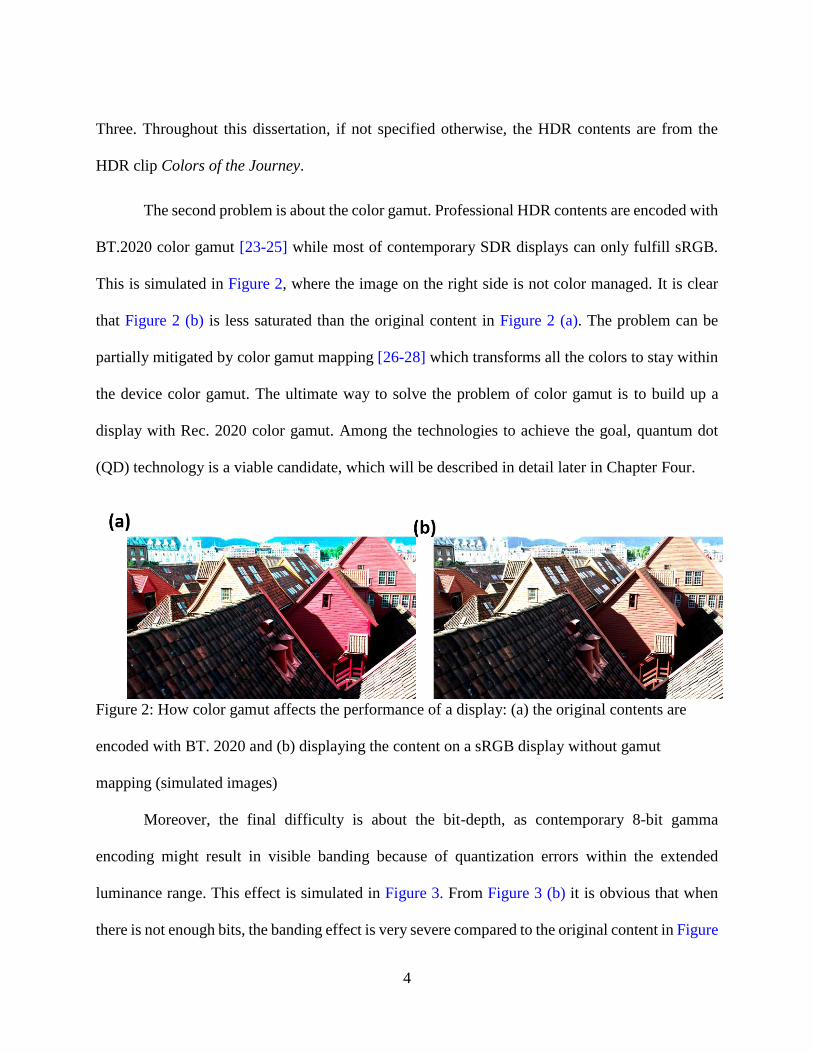
The second problem is about the color gamut. Professional HDR contents are encoded with

BT.2020 color gamut [23-25] while most of contemporary SDR displays can only fulfill sRGB.

This is simulated in Figure 2, where the image on the right side is not color managed. It is clear

that Figure 2 (b) is less saturated than the original content in Figure 2 (a). The problem can be

partially mitigated by color gamut mapping [26-28] which transforms all the colors to stay within

the device color gamut. The ultimate way to solve the problem of color gamut is to build up a

display with Rec. 2020 color gamut. Among the technologies to achieve the goal, quantum dot

(QD) technology is a viable candidate, which will be described in detail later in Chapter Four.

Figure 2: How color gamut affects the performance of a display: (a) the original contents are

encoded with BT. 2020 and (b) displaying the content on a sRGB display without gamut

mapping (simulated images)

Moreover, the final difficulty is about the bit-depth, as contemporary 8-bit gamma

encoding might result in visible banding because of quantization errors within the extended

luminance range. This effect is simulated in Figure 3. From Figure 3 (b) it is obvious that when

there is not enough bits, the banding effect is very severe compared to the original content in Figure

5

3 (a). Currently the display industry is using the dithering process [29], which deliberately adds

noise to the image to mitigate the banding effect and improve image quality. However, from Figure

3 (c) it is illustrated that the color banding cannot be fully suppressed. That is why the industry is

moving towards a 10-bit solution. Going even a step further, a legitimate goal will be to build a

12-bit display based on the perceptual quantizer (PQ) curve [30], also known as the ST. 2084

standard that covers from 0 to 10,000 nits. In Chapter Five, we will present our scheme to achieve

the 12-bit PQ curve based on a local dimming LCD system.

6

Figure 3: How bit-depth affects the performance of display: (a) the original content with 24 bits

in total, (b) displaying the content on a display that only supports 256 colors, and (c) the

dithering process to mitigate the banding effect. (Simulated images)

Besides the hardware limitations, another problem is that the current display processing

pipeline treats HDR content the same way as it treats the SDR content. After decoding to linear

RGB, contemporary display processing pipeline transforms from linear RGB to XYZ through

Equation (1):

.

X R

Y LM G

Z B

(1)

Here L is the luminance factor based on the display brightness and M is the color transformation

matrix that can be retrieved from the display profile. For a sRGB display:

0.412424 0.357579 0.180464

0.212656 0.715158 0.0721856 .

0.0193324 0.119193 0.950444

M

(2)

With this approach, RGB values smaller than or equal to unity are transformed as is, while

RGB values larger than unity are clipped to one. In this way, a RGB value of (1,1,1) is transformed

to display white.

While this pipeline works well with SDR content, for HDR content it can distort the

creator’s intention, as demonstrated in Figure 4 (a). This image is a frame from the HDR trailer of

Life of Pi. Much of the scene is interpreted as white and it appears that the actor is travelling under

direct sunlight. However, as demonstrated in Figure 4 (b), which is a tone-mapped version of the

original scene via highlight compression, the real intention of the creator is that the actor is actually

7

travelling at sunset or sunrise. In this sense, the contemporary approach in displaying HDR content

could incorrectly render the creator’s intention.

Figure 4: (a) How HDR content are currently displayed on SDR devices, and (b) the real

intention of the creator (tone mapped version of the original image)

The reason that contemporary display principle does not work is that for HDR content, the

linear RGB values can go beyond unity. For example, for Figure 4 , this clip has a luminance factor

L of 80 and reference white is 80 nits. In this way, the grayish clouds area (with RGB values

around 2) is actually ~160 nits while contemporary display “interpret” that they are beyond display

peak brightness and clipped them to display white.

To solve this problem, we propose a new HDR gamut mapping approach to display HDR

contents adaptively based on the display specifications, this part will be discussed in Chapter Six.

8

CHAPTER TWO: HIGH AMBIENT CONTRAST AUGMENTED REALITY

SYSTEMS

The device configuration of Google Glass, a typical AR system is shown in Figure 5. It

consists of a display system, a collimating lens system, and a PBS. The PBS partially reflects the

display light and transmits the ambient light. It is obvious from the schematic view that the PBS

makes the whole system bulky.

Figure 5: Working principle of Google Glass

Besides system compactness, another problem associated with the PBS is its ambient

contrast ratio (ACR). The following equation [11] can be used to determine how much light can

be transmitted by the PBS:

( ) ( ) .i i iL It d (3)

Here i=x,y represents the x and y polarization, respectively, t(λ) is the wavelength dependent

transmittance and I(λ) is light spectral power distribution (SPD). Most of the time the ambient light

is unpolarized, thus Equation (3) can be simplified as:

9

( ) ( )1

[ (2

.)]a yxtL t I d (4)

Here a stands for ambient light. Similarly, the total reflected display light is:

( ) ([ ) ( )]) ( .D Dx Dyx yL I r I dr (5)

Again rx=1-tx and ry=1-ty is the wavelength dependent reflectance of the PBS, respectively and D

stands for the displayed light. For simplicity, we will assume I is constant across the wavelength

and r=t=0.5. In this way for OLED display where the display light is unpolarized [31] and LCD

where the display light is linearly polarized, the ACR can be written as:

.Don a Don a

Doff a Doff a

IL L IACR

L I IL

(6)

Here on and off means the on and off states of the display. For an ideal AR system, we want the

display light and the ambient light to fuse together, thus making the viewing experience immersive.

For this purpose, IDon should be close to Ia. A typical outdoor display today has a peak luminance

of ~2000 nits whereas in broad daylight the luminance of the ambient light can easily go over

20000 nits. Such high luminance will deteriorate the display image.

From Equation (6), it is quite straightforward that there are two ways to improve the ACR:

improving the display brightness or attenuating the ambient light. Because of power consumption

and lifetime [19] concerns, further improve the display brightness to beyond 20000 nits is not

feasible. Thus leaving us to the only solution of attenuating the ambient light level. This is exactly

the concept we utilized in our AR system.

10

2.1 A high ambient contrast augmented reality system

The device configuration of our AR system is shown in Figure 6: the tunable

transmittance LC film is laminated on the front surface of the eyeglasses and the reflective

polarizer/functional reflective polarizer is laminated on the back surface of the eyeglass.

For the polarized display, a possible choice is a liquid crystal on silicon (LCOS) [32-34]

pico-projector with an output angle range of ±15°.

Figure 6: Device configuration of our high ambient contrast system.

The tunable-transmittance LC film is tuned electronically and pairs together with an

ambient light sensor so that the LC film is clear at low lux level and it turns to a dark state

at high ambient light conditions, thus ensuring a high ACR under all conditions. Because

of this we call the film as a smart dimmer. The performance of the tunable transmittance

LC film will be discussed later in this chapter. The reflective polarizer, also known as dual

brightness enhancement film (DBEF) [11-13], works the same way as the PBS by reflecting

one polarization while transmitting the other. The main advantages of the reflective

polarizer are twofold: its size can be much larger and its weight much lighter than those of

11

PBS. Moreover, if we replace the reflective polarizer with our specially designed functional

reflective polarizer, such system can help people with CVD, more precisely people with

anomalous trichromacy [35, 36]. The design and performance of the functional reflective

polarizer will also be demonstrated later. Besides AR systems, our device can also be

laminated to the windshield for high ACR vehicular displays.

2.2 The tunable transmittance LC film

A tunable transmittance system is desirable for applications where the ambient light is

strong, for example, outdoor displays, energy efficient smart windows and car windshields.

Several approaches have been developed to achieve tunable transmittance. Among these

approaches, the most mature and commercially successful approach is the photochromic materials.

[37] used in transition glasses. However, besides their exceptional performance, transition glasses

often suffer from sluggish response time, as measured in Figure 7. In our experiment, we irradiated

UV light onto a commercial transition glass and measured its time-dependent transmittance. As

Figure 7 (a) depicts, the transmittance drops from ~83% to ~10% in 30s. As soon as the UV lamp

was turned off, the transmittance changes back to ~83% gradually in 25 min [Figure 7 (b)]. While

for the eye response, the pupil regulates the amount of light entering the eye cavity by changing

its diameter, taking between 2-5 s to complete the process [38]. The retina on the other hand needs

within 1-2 min to adapt completely to the new lighting state through activation and deactivation

of photoreceptor cells [38]. It is clear that the transition glass is not as fast as the human visual

system. Such a slow response time is not practical for AR systems and thus we proposed a fast-

response tunable transmittance LC film.

12

Figure 7: Time-dependent transmittance of a commercial transition glass: (a) from bright state to

dark state and (b) from dark state to bright state.

Our voltage-driven tunable transmittance LC film is powered by AlphaMicron’s e-Tint

technology based on the guest-host approach [39]. In this approach, the LC host (Δε<0) is doped

with ~3% black dichroic dyes and a small amount of chiral agent. The working principle of the

guest-host LC cell is illustrated in Figure 8. The LC directors are in pink and the dichroic dyes are

in black. At zero volt, the LC directors and dichroic dyes are homeotropically aligned and the

absorption loss of the incident white light is minimal. Thus, the LC cell is highly transparent. Once

the voltage exceeds a threshold, the LC directors and dichroic dyes are reoriented by the electric

field to form a 180° super twisted nematic (STN) mode [40] because of the doped chiral agent

Such a 180° STN guest-host structure absorbs the incident light strongly and the effect is

insensitive to the polarization of the incident white light. The detailed mechanisms of such a chiral-

homeotropic cell (without dyes) has been described in [40].

13

Figure 8: Working principle of the tunable transmittance LC film at (a) bright state and (b) dark

state.

The voltage-dependent transmittance of our LC cell is shown in Figure 9: from the bright

state (V=0) to the dark state (8V), the transmittance varies from ~73% to ~26%. With an embedded

ambient light sensor, the LC film can control the transmittance adaptively according to its

brightness. As a result, it helps to obtain high ACR. Besides the tunable transmittance, the

measured turn-on time (bright to dark) is 3.8 ms and turn-off time (dark to bright) is 50.5 ms. Such

response time is at least 10X faster than that of transition glasses and is sufficient for eyewear

applications.

14

Figure 9: Voltage dependent transmittance of the LC film

The response time τ of the display can be estimated by

2

1

2.~

d

K

(7)

Here γ1 is the rotational viscosity, K is the effective elastic constant and d is the cell gap. To further

reduce the response time of the LC film, we can use a lower viscosity LC or optimize the cell gap.

The ultimate goal of a see-through AR system is to connect the virtual world and the real

world. This means the “dark” state of the LC cell cannot be completely black, and our LC film can

successfully achieve this purpose, as demonstrated in Figure 10 (a) and (b). The photos were taken

under normal indoor lighting. From Figure 10, we can tell that the LC cell is quite clear at the

bright state (V=0). At the darkest state (8 Vrms), although the transmittance drops we can still

distinguish the RGB colors clearly.

15

Figure 10: The performance of the LC cell at (a) bright state and (b) dark state.

Another advantage of our smart dimmer is that this film is fail-safe: when no voltage is

applied, the device is in bright state, which ensures high visibility of the ambient environment even

when the electronics go wrong. This ensures the users’ safety.

2.3 Design Principle of the functional reflective polarizer

The Reflective polarizer, which can be mass-produced by polymer coextrusion [41], has

been widely used in LCD backlight for polarization manipulation and recycling. It consists of

hundreds of stacked isotropic and uniaxial layers, as shown in Figure 11 (a). The refractive index

of the isotropic material is n1, as for the uniaxial material the ordinary refractive index is n1 and

the extraordinary refractive index is n2. The uniaxial material is aligned along the x-axis. For the

light polarized along the x-axis, it sees alternating refractive index and the stack works as a highly

reflective film. While for the light polarized along the y-axis, it sees only n1 so that the structure

works as a high transmittance film. In this way, the reflective polarizer would reflect the x-

polarized light while transmitting y-polarized light. The reflective polarizer can be designed by the

4×4 method [42, 43] developed for analyzing uniaxial liquid crystals. However, as there is no

refractive index change along the y direction, it is not possible to control the

transmittance/reflectance of the y-polarized light. The most straightforward way to control the

transmittance/reflectance of the y-polarized light is to introduce refractive index variation in the y

16

direction. However, designing such a functional reflective polarizer that controls the x-polarized

light and y-polarized light simultaneously is quite challenging by the 4×4 method. To help design

the functional reflective polarizer, we need to take a look at the 4×4 method, which is used for

analyzing liquid crystal display, and the transfer matrix approach [44], which is used in general

for thin film coating design. We can tell that the main difference between the transfer matrix

approach and the 4×4 method is that in the latter we introduce polar and azimuthal angles to

describe the tilt and twist deformations of the LC directors. The incurred LC reorientation will

introduce polarization rotation effect into the system. However, in the case of functional reflective

polarizer, the problem can be greatly simplified if we assume that the uniaxial material is oriented

along x-axis or y-axis. Then the polarization rotation effect would be negligible and the design

process of the functional reflective polarizer can be simplified as outlined in the following:

1. Designing two thin film coatings with different transmittance/reflectance properties

using isotropic materials m1 and m2 with refractive index n1 and n2, respectively. If we

name the two coatings Stack 1 and Stack 2, it is required that the two thin film coatings

having the same thickness.

2. Convert the two thin film coatings to functional reflective polarizer. Compare the two

stacks: at the same thickness, if both stacks have the refractive index of n1, then for the

functional reflective polarizer, at this thickness we should use material m1. Similarly,

if both stacks have the refractive indices of n2, we should use isotropic material m2. In

addition, if for Stack 1 the refractive index is n1 and for Stack 2 the refractive index is

n2, then we should use the uniaxial material m3 (ne=n2 and no=n1) with the long axis

aligned along the y direction. If on the contrary, the refractive index for Stack 1 is n2

17

and for Stack 2 the refractive index is n1, then the uniaxial material should be aligned

along the x direction. This conversion procedure is illustrated in Figure 11 (b).

3. Recalculate the transmittance and reflectivity of the functional reflective polarizer with

the 4×4 method.

4. Fine-tune the stack design of the functional reflective polarizer.

Figure 11: (a) Structure of the regular reflective polarizer and (b) the principle of converting two

thin film coatings to a single functional reflective polarizer: materials m1, m2 and m3 are drawn

in white, blue and yellow, respectively.

With the abovementioned approach, it is possible to design the functional reflective

polarizer with three materials: a uniaxial material with ne=n2 and no=n1 and two isotropic materials

with matched refractive indices of n1 and n2, respectively. The isotropic materials we used in our

18

design simulation are NOA81 (n=1.57) [45] and polyferrocenes (n=1.82) [46], and the uniaxial

material is liquid crystal polymeric film (BL038, ne=1.82, no=1.57) [45]. In real fabrication, we

can also select other materials as long as the refractive index matching condition is satisfied and

the birefringence of the uniaxial material is large enough. The most important advantage of our

approach is that there are quite a few optimization approaches for fast thin film coating designs.

2.4 Functional reflective polarizer embedded AR system for color vision deficiency

With the abovementioned approach, we designed an AR system with functional reflective

polarizer for helping people with color vision deficiency (CVD). For this kind of application, the

design process is mentioned in the previous section. Before we dig into the design principle, we

will first give a brief introduction of color vision deficiency.

2.4.1. Origin of color vision deficiency

In the retina of the human eye, there are three types of cone cells that contribute to color

vision: the L, M and S cone cells. Here L, M and S stands for long-wave, medium wave and short

wave, respectively. For people with normal vision, the spectra sensitivity of their cones cells are

shown in Figure 12. There are three types of CVD: 1) anomalous trichromacy where one of the

pigments have shifted or altered spectra sensitivity; 2) dichromacy where one of the cone cells are

not present or not working and 3) monochromacy where the viewer cannot distinguish colors [11,

14, 15]. In our thesis, we will only talk about anomalous trichromacy. A simple explanation for

anomalous trichromacy is that one type of the cone cells are partially contaminated by another

type, thus resulting in a spectra shift in the sensitivity curve. Depending on which kind is

contaminated, there are three types of anomalous trichromacy: protanomaly, deuteranomaly, and

tritanomaly. For example, in Figure 12, the red dashed lines represent a case of protanomaly where

19

the spectral sensitivity of the L cone cells shifts by 10nm. The larger overlap between the spectra

sensitivity functions of the L and M cone cells results in inaccurate color perception.

Figure 12: Spectra sensitivity functions of the L, M and S cone cells and the transmittance of the

commercial EnChroma glasses for people with CVD.

The severity of anomalous trichromacy can be described by [36]:

.20

S

(8)

Here Δλ is the spectral shift in nm. From Equation (8), when S=1, i.e. Δλ=20nm, which implies

that two of the spectra sensitivity functions completely overlap. It means the patient is with

dichromacy and can only perceive two primary colors.

To help people with CVD, both computer vision based approach [36] and optics based

approach have been proposed. For the latter, the basic principle is to use notched filters to reduce

the overlap between the spectra sensitivity functions of the L, M and S cone cells. Also included

in Figure 12, the black line is the measured transmittance data of a commercial EnChroma glass

designed for people with CVD. It is obvious that there are three transmittance dips along the black

20

curve, and these transmittance dips help to reduce the overlap between adjacent spectra sensitivity

functions.

2.4.2. Performance of our functional reflective polarizer

In our functional reflective polarizer-embedded AR system, both computer algorithm and

optical approaches can be applied to help people with CVD. For the x-polarized display light, the

display can be tailored based on computer algorithms to adapt to the viewer. The reflectance of

the functional reflective polarizer in the x direction should be as high as possible, thus it will not

temper the output display spectra and cause color inaccuracy of the displayed images. For the

incident ambient light, the x-polarized part will be reflected back and cannot be perceived by the

viewer. While for the y-polarization, the functional reflective polarizer functions as a notched filter

to reduce the overlap between adjacent spectra sensitivity functions. Thus, the functional reflective

polarizer can optically adapt the environment light for people with CVD. Based on the approach

shown in Figure 11 (b), we have designed the functional reflective polarizer with its transmittance

shown in Figure 13. Here we use all three materials listed in previous section. The reflective

polarizer consists of 793 layers with a total thickness of 30.03 µm. Again, the thickness and

alignment of each specific layer are not shown here. From Figure 13 it is obvious that our

functional reflective polarizer has low transmittance (high reflectivity) for the x polarization across

the visible range and it works as a notched filter simultaneously in the y direction. The overall

reflectivity RD of the x-polarized display light can be defined as:

1 ( ) ( ) / ( )1 .D D x D Dt I d I dR T (7)

In Equation (7), TD is the overall transmittance of the display light and ID(λ) is the spectra of the

display light. The overall reflectivity RD of the x-polarized display light calculated from Equation

21

(7) is ~99.0%. This indicates that with our functional reflective polarizer, both the display light

and ambient light can be tailored to help those people with CVD.

.

Figure 13: Spectra sensitivity function of the L, M and S cone cells and the transmittance of our

functional reflective polarizer in the x and y polarization.

To evaluate the performance of our functional reflective polarizer, we simulate the images

perceived by people with anomalous trichromacy with and without the functional reflective

polarizer. The simulation is powered by the open source isetbio Toolbox [47] and the simulation

approach is well documented in [36]. Here we summarize it as follows: 1) we obtain the RGB

values of each image pixel. By specifying the light source, we can further get the spectra of each

image pixel through the isetbio Toolbox. 2) We can simulate the perceived spectra of each pixel

after the functional reflective polarizer. Then an image perceived by people with normal vision

can be reconstructed based on the spectra. For people with anomalous trichromacy, the perceived

image can be deduced from the image perceived by people with normal vision based on matrix

manipulation described in [36]. Here we assume the ambient environment is a close-up view of a

22

ladybeetle. The simulation image is taken from Wikimedia Commons and here we assume the

image is displayed by the OLED panel specified as “OLED-Samsung.mat” in the isetbio Toolbox.

In our simulation, we consider two cases: (1) the severity of anomalous trichromacy is 0.4 (8nm

spectral shift), which means the anomalous trichromacy is not very severe and (2) the severity of

anomalous trichromacy is 0.8 (16nm spectral shift) where the CVD is quite severe. For the first

case, the simulation results without and with the functional reflective polarizer are illustrated in

Figure 14 (a) and (b), respectively. Our functional reflective polarizer helps people with anomalous

trichromacy to see more saturated colors when the anomalous trichromacy is not severe. For the

second case, the perceived images without and with functional reflective polarizer are

demonstrated in Figure 14 (c) and (d), respectively. By comparing these two figures, we find that

even when the anomalous trichromacy is severe our functional reflective polarizer is still helpful

to enhance the image contrast.

23

Figure 14: (a) The perceived image without functional reflective polarizer. From upper left to

bottom right, the images correspond to people with normal vision (upper left), protanomaly

(upper right), deuteranomaly (bottom left) and tritanomaly (bottom right); (b) the perceived

image with functional reflective polarizer. For (a)-(b), the spectral shift is 8nm. (c) The perceived

image without functional reflective polarizer when the spectral shift is 16nm and (d) the

perceived image with functional reflective polarizer when the spectral shift is 16nm.

2.5 Summary

In summary, we have developed a high ACR AR system for people with CVD by

combining a smart dimmer with a functional reflective polarizer. The smart dimmer is based on

the guest-host LC approach and has three advantages: 1) fast response time, 2) high ambient

contrast and 3) fail-safe. The design principle of the functional reflective polarizer is well

24

explained. The functional reflective polarizer demonstrates high reflectivity in one polarization

and works as a notched filter in the other polarization.

25

CHAPTER THREE: DUAL PANEL FOR HIGH DYNAMIC RANGE

DISPLAYS

As mentioned in Chapter One, to achieve high dynamic range we should improve the dark

state and peak brightness of the display simultaneously. For example, the luminance of bright state

should be > 1000 nits, while dark state should be < 0.01 nits. In other words, the effective CR is

over 100,000:1. For an organic light-emitting diode (OLED) display, it is fairly easy to get true

black state, but to obtain a brightness over 1000 nits would lead to compromised lifetime [48]. On

the other hand, with the help of high power LEDs, it is relatively easy to boost an LCD’s peak

brightness to 1000 nits, but to lower the dark state to < 0.01 nits is challenging. A typical CR of a

multi-domain vertical alignment (MVA) LCD is ~5000:1, which is about 20x lower than what

HDR demands. To improve dark state, local dimming technique has been commonly used [49, 50].

A key challenge with the present local dimming approach is that it cannot be pixelated,

thus requires complex algorithms [51] to mitigate the image artifacts, such as halo and clipping.

To avoid the computational complexity, a pixel-by-pixel local dimming approach is preferred.

In this chapter, we demonstrate a HDR LCD with two cascaded panels. In fact, dual-layer

or even multi-layer LCD has already been widely used in 3D display, volumetric display and light

field display [52-54], but few reports are focused on their electro-optical properties. Here, we

perform systematic investigations on the dual-panel HDR LCD system, with special emphases on

contrast ratio, operation voltage, response time, viewing angle, and Moiré effect. Our analysis and

test cell experimental results indicate that we are able to achieve CR >1,000,000:1 (limited by the

noise of our photodiode detector), low operation voltage (~5V), and pixel-level local dimming. To

eliminate the Moiré patterns induced by the cascaded TFT backplanes, we introduced a

26

polarization dependent scattering film (PDSF). Potential concerns for the dual-layer system are

discussed, such as increased panel thickness, weight, cost, misalignment effect, and reduced

optical efficiency. We believe such a HDR LCD would find widespread applications for medical

imaging, art designing, movies, and vehicular displays.

3.1 Device configuration and working principles

The device configuration of the dual panel system is shown in Figure 15. The system

consists of a master display panel (LCD #2) and a pixelated dimming panel (LCD #1). In principle,

any two LC modes can be paired up to construct the display [55-57], for example, VA and 90° TN

(twisted nematic), VA and FFS (fringe-field switching), FFS and TN, two TNs, or two FFSs, just

to name a few. However, considering the viewing angle, color shift, and cost, we choose FFS as

master display and black-and-white TN (the same dimension but without color filters) as local

dimmer. TN is a normally-white broadband half-wave plate [56], that means, at V = 0 the incident

white light passes through the TN panel and reaches the master display with high efficiency. If the

local dimming is on demand, we can apply different voltages (through TFTs) to those chosen

pixels to control their transmittance. While for the FFS panel, it shows excellent image quality,

including wide viewing angle, small color shift, weak gamma shift, and pressure resistance for

touch panels. Therefore, we put it in the viewer side. Later, we will use the FFS/TN test cell results

to illustrate the operation principles. Let us assume the contrast ratio of the two LCD panels is CR1

and CR2, respectively. Then for the cascaded display system, the effective contrast ratio should be

CR1*CR2 [1]. A typical CR for FFS LCD is ~2000:1 and TN is ~800:1, thus ideally the intrinsic

CR of dual panels should be 1,600,000:1. Another advantage of this design is pixel-level local

dimming, similar to OLED, if two panels are aligned well. Of course, there are some drawbacks,

27

like decreased efficiency, increased cost, and misalignment issue. We will discuss these factors in

detail later.

Figure 15: Device setup of the dual panel display system.

3.2 simulation and experimental results

Based on the dual panel concept, we conducted simulation and experimental analysis.

Below are the results:

3.2.1 VT Curve

In experiment, we prepared one TN test cell with cell gap d = 5 µm and one FFS test cell

with cell gap d = 3.5 µm. The employed LC (MLC-6686, Merck) material parameters are:

birefringence Δn = 0.0983 @ λ = 550 nm and dielectric anisotropy Δε = 10.0 [58] A He-Ne laser

with λ = 633 nm was used as probe beam. During measurement, the LC cell was driven by a square-

wave voltage at 1 kHz frequency. The applied voltage was controlled by a LabVIEW (National

28

Instruments) system. The measured voltage-dependent transmittance (VT) curves for both cells

are plotted in Figure 16. As expected, the TN test cell shows ~100% transmittance (normalized to

two parallel polarizers) and the dark state occurs at V = 3 Vrms. It is a perfect candidate for backlight

local dimming. While for the FFS test cell (electrode width = 4 µm, and electrode gap = 3 µm), its

peak transmittance at λ = 633 nm is 73.6% and Von = 4.2 V. If a low Δε LC mixture is employed,

higher transmittance can be obtained, but at a slightly higher voltage [58].

Figure 16: Voltage-transmittance curve measurement of the TN and FFS cell.

3.2.2 Contrast ratio

Next, we measured the contrast ratio of these two test cells. Results are CRFFS = 4625:1 and

CRTN = 2172:1. When we placed these two cells in sequence (TN is closer to the light source), in

principle the CR should reach 9,263,580:1 (CRFFS*CRTN), but in experiment we only obtained CR

= 1,102,564:1 when the TN cell was driven at 3 Vrms. This result is 8.4x smaller than the theoretical

value, but still much higher than the required 100,000:1 requirement for HDR displays. The

reduced CR could be limited by the sensitivity of the photodiode detector we employed. Please

29

note that, here, high extinction ratio (~ 18,000:1) polarizers were adopted, and the measurement

was performed using He-Ne laser (λ = 633 nm). As a result, the obtained CR would be higher than

the traditional value using white backlight.

3.2.3 Response time

The measured response time of the FFS and TN cell is shown in Figure 17 (a) and (b),

respectively. Due to the small twist elastic constant [59], FFS cell exhibits relatively slower

response time (rise time: 24.5 ms, decay time: 21.6 ms); while for TN cell, the measured response

time is fairly fast (decay time: 4.4 ms, rise time: 9.7 ms). Then we combine FFS and TN cell

together, and investigate the response time of dual-panel system. Results are plotted in Figure 17

(c), where rise time is 19.0 ms, and decay time is 6.4 ms. Interestingly, both rise and decay time

are improved as compared to single FFS cell, especially for decay time (21.6 ms vs. 6.4 ms). It

means TN panel helps to accelerate the total transition process efficiently. If we use a thinner cell

gap with higher Δn yet low viscosity LC, faster response time (< 2 ms) can be realized [60-62]. In

this way, the motion picture response time of the display would be comparable to that of an OLED,

leading to much suppressed image blurs. [63, 64].

30

Figure 17: Measured response time for (a) single FFS cell, (b) single TN cell, and (c) combined

FFS + TN cell.

3.2.4 Viewing angle

Figure 18 (a) shows the simulated isocontrast contours for a conventional TN LCD. The

highest CR is about 1200:1, and it drops gradually as the viewing cone increases. For some

azimuthal angle, say 230°, it is less than 10:1, which means the image quality is degraded greatly.

For FFS LCD [Figure 18 (b)], its CR could reach ~2500:1, but still drop to 100:1 at large viewing

angles.

31

Figure 18: Calculated isocontrast contour for (a) single TN panel and (b) single FFS panel.

When we cascade them together, the CR exceeds 1,000,000:1 within the ~20° viewing cone,

as shown in Figure 19. Even for the entire viewing zone, CR still keeps over 1000:1. If we define

the HDR requirement as 100,000:1, then the viewing angle in the horizontal direction is extended

to about 60°. Meanwhile, since we use FFS as master display panel, its color shift and gamma shift

are very weak.

Figure 19: Simulated isocontrast contour for the cascaded FFS and TN panels.

3.3 Potential problems of the dual panel approach

As above mentioned, dual LCD panels show great advantages in contrast ratio and viewing

angle. However, some challenges remain to be solved. The first one is increased cost, because two

panels are used. Fortunately, the portion of panel cost in total price is not high. For example, in a

32

5’’ FHD smartphone, the LCD panel is only $25 or lower. Compared to the total price $500 of a

smartphone, the display part only occupies ~5%. For large size TVs, this portion is higher, but still

acceptable. On the other hand, cost is not a big issue for some high-end devices, like medical

diagnosis, movie directing, photographers, universe detecting, art designers, etc.

Increased thickness is another concern for dual LCD panels. For a conventional edge-lit

LCD panel, the thickness is about 1.6 mm. And for direct-lit technology with local dimming,

thickness is ~5 mm. As shown in Figure 15, in our design, one more LC panel is added, consisting

of two polarizers (130 µm × 2), two substrates (200 µm × 2), LC layer (4 µm), and compensation

films (150 µm). The total thickness is about 0.9 mm. Therefore, for the whole device it is 2.5-mm

thick, which is still ~2x thinner than the direct-lit display.

The other issue for dual LCD panels is decreased efficiency, which mainly results from the

additional polarizers. Because of the absorption of polarizer, about 25% optical efficiency is

sacrificed. At the same time, the electrical power consumption would increase or even doubled as

compared to a single panel.

Next issue is misalignment. If two LC panels do not align precisely, then the image would

be distorted. Fortunately, this issue could be mitigated from image processing part. Guarnieri et al.

developed a novel splitting algorithm to minimize the errors caused by misalignment [65, 66].

Based on their analysis, the images could still remain good quality even though there is 3-pixel

spatial shift between two LCD panels.

3.4 Reducing the Moiré effect with polarization dependent scattering film

When two LCD panels are placed in sequence, Moiré effect appears because of the

patterned TFT backplanes. To reduce this effect, a strong diffuser is often needed. In this case, the

33

output light from the first panel will be depolarized, degrading the whole performance. To solve

this issue, we proposed a new structure design using a polarization dependent scattering film

(PDSF), as depicted in Figure 20. The only difference is that a PDSF is added between two LCD

panels, to replace the conventional strong diffuser. This PDSF exhibits a unique property:

polarization dependent scattering [67, 68]. For example, PDSF would scatter the s-wave strongly,

whereas transmitting the p-wave. With this unique scattering property of PDSF film, Moiré effect

would be mitigated while keeping high CR for dual LCD panels.

The working mechanism could be briefly described as follows. For bright state, there is

strong s-polarized light from the first LCD panel. As described above, it would be scattered by the

PDSF, then entering the second LCD panel. As a result, Moiré effect is mitigated. While for dark

state, quite weak p-polarized light traverses through the first TN panel, and enters PDSF. In this

case, it could go through without scattering; its polarization state is conserved. Namely, no

depolarization effect occurs. Thus, high CR is realized. Clearly, in real applications, the

transmittance and scattering properties of PSDF need to be optimized in order to balance the Moiré

effect reduction and high contrast ratio.

34

Figure 20: Schematic diagram for the proposed structure using polarization dependent scattering

film (PDSF).

Experimentally, we prepared a mixture consisting of BL038 (95.6 wt%), RM257 (4.2 wt%)

and Irg651 (0.2 wt%). Homogeneous cell with cell gap d = 12 µm was employed. Then LC test

cell was first cured using 365 nm UV lamp for 30 sec with 5 mW/cm2. After that, we applied 20

V to the cell, and cured again for 1 hour with the same UV intensity. The detailed fabrication

process and physical mechanism of PDSF could be found in [22]. The measurement setup is

depicted in Figure 21. A He-Ne laser with λ = 633 nm was used as probing beam and the acceptance

angle of detector was 4.5°.

Figure 21: Experimental setup for PDSF measurement.

35

When we rotate the PDSF, the light intensity after PDSF is changed because the scattered

or transmitted light is tuned. The measured result is plotted in Figure 22. The peak transmittance

is 75%, while in the scattering state the transmittance drops to 2.6%. The CR is about 28.6:1. Also,

we compared their spectrum at two states, as shown in Figure 23. As the wavelength decreases,

the scattering gets stronger, leading to decreased transmittance. For practical applications, the

recipe of PDSF and its curing conditions have to be optimized based on different requirements.

Figure 22: Transmittance as a function of polarization angle.

Figure 23: Measured transmission and scattering spectra of the PDSF.

3.5 Summary

In summary, to solve the contrast ratio challenge of HDR display. We have proposed a

dual panel approach. Besides high contrast, the system has the advantage of pixel level local

0 20 40 60 80 100 120 140 160 1800.0

0.1

0.2

0.3

0.4

0.5

0.6

0.7

0.8

Tra

nsm

itta

nce

Angle (o)

36

dimming. The challenges of this approach, such as the misalignment issue and system compactness

are also discussed. At the same time, the PDSF approach has been investigated and analyzed to

suppress the Moiré effect.

37

CHAPTER FOUR: QUANTUM DOTS FOR WIDE COLOR GAMUT HIGH

DYNAMIC RANGE DISPLAYS

As mentioned in Chapter One, HDR displays also come with more saturated colors. The

color a display can present is described by the color gamut. The color gamut is described as the

triangle confined by the color primaries in the CIE1931 color diagram. A larger color triangle

indicates the display can produce more saturated colors. Among these color gamuts, some of the

most widely used color gamuts are: sRGB, which is the de-facto standard for online images; Rec.

709, which is a variety of sRGB standardized for high definition TV (HDTV) [69]; DCI-P3, which

has been used by the entertainment industry and is gaining momentum in consumer electronics

[70]; Adobe RGB, which is quite popular among professional photographers because of its deep

and saturated green colors [71]; and the latest Rec. 2020 color gamut [23]. The Rec. 2020 color

gamut became the standard for ultra-high definition (UHD) and HDR displays for three reasons:

1. The Rec. 2020 color gamut can enclose the color primaries of all the other four standards [72];

2. The color triangle of Rec. 2020 cover up to 99.9% of the Pointer’s gamut [73], which indicates

displays capable of handling Rec. 2020 can faithfully reproduce the natural object colors. Finally

yet importantly, the Rec. 2020 standard can be physically realized through RGB laser sources [72,

74]. These color gamuts are plotted in Figure 24.

38

Figure 24: Typical color gamuts used in display industry.

Although the Rec. 2020 standard can be realized with monochromatic laser sources, for a

real display, laser sources are expensive and the speckle problem [75] has not yet been fully solved.

In this sense, it is preferred to find non-monochromatic light sources to realize the Rec. 2020

standard. Among these candidates, quantum dots (QDs) have attracted much attention because of

their narrow and tunable emission spectra [76].

There are two approaches to use QDs for displays: photoluminescence (PL) quantum dots

for liquid crystal display (LCD) backlight [25, 77, 78] and electroluminescence (EL) quantum-dot

light emitting diodes (QLEDs) [31, 79-82]. In this thesis, we will discuss how to realize the Rec.

2020 standard with both approaches, and the tradeoff between color gamut and optical efficiency.

39

4.1 Display system evaluation

Before we dive into performance evaluation of different displays, we should first establish

the evaluation metrics. The first and most important evaluation metric is color gamut, which is

determined by the maximum colors a display can reproduce based on Rec. 2020. While the system

colorimetry of Rec. 2020 [23] shown in Table 1 is quite straightforward, the definition of color

gamut is sometimes confusing and misleading. The most accurate way is to calculate the color

volume in a three-dimensional (3D) color space or color appearance model, such as the CIELAB

or CIECAM02. However, the gamut calculation in 3D color space is both complex and unintuitive

and no one actually do this in the display industry. Instead, the gamut calculation is based on two-

dimensional (2D) color diagrams. Some manufactures define the area ratio as the color gamut,

which compares the RGB triangular area of a display with the triangular area of the Rec. 2020

standard, namely:

.display

standard

AColor Gamut Area

A (8)

Whereas others define the coverage ratio as the color gamut, which can be expressed as:

.display standard

standard

A AColor Gamut Area

A (9)

What makes the situation even more confusing is that CIE 1931 and CIE 1976 are used

simultaneously when calculating the color gamut, although these two color spaces are quite

different. As pointed out in [24] the coverage ratios in CIE 1931 and CIE 1976 are rather

inconsistent, and the coverage ratio calculated with CIE 1931 is more consistent to the Rec. 2020

volume coverage ratio in color appearance model CIELAB, CIELUV and CIECAM02. In this

40

sense, we will use the coverage ratio in CIE 1931 as the metric, while including the coverage ratio

in CIE 1976 as a reference. We will discuss more about the color space selection later in this

chapter.

Table 1: System colorimetry of Rec. 2020 standards

Primary

colors and

Reference

white

Chromaticity

coordinates

(CIE 1931)

x y

Corresponding

wavelength

(nm)

Red Primary 0.708 0.292 630

Green

Primary 0.170 0.797 532

Blue

Primary 0.131 0.046 467

Reference

White (D65) 0.313 0.329 /

The other metric should describe how efficient the display system is. Here we emphasize

on optical efficiency because realizing a wide color gamut is mainly to optimize the output spectra

power density (SPD). The SPD directly determines the luminous efficacy of radiation (LER) of

the system [77]:

( ) ( ).

( )

m out

out

K V dLER

d

S

S

(10)

In Equation (10), Sout (λ) is the SPD of the output light, V(λ) is the standard luminosity function,

and Km=683 lm/W is the LER of the ideal monochromatic 555-nm source. As the LER is only

determined by the light spectra, it sets the theoretical limit for the total efficiency of a display.

For a non-emissive display such as LCD, the SPD of the backlight (Sin(λ)) and the actual

output light (Sout(λ)) can be modulated dramatically, depending on the transmission characteristics

of the system. To quantify the transmission characteristics of the system, we introduce the transfer

efficiency (TE) of the system as:

41

( ).

( )Sout

in

dTE

d

S

(11)

The total light efficiency (TLE) of the system is:

( ) ( ).

( )Sm out

in

V dTLE LER TE

d

K S

(12)

For our analysis below, the main evaluation metrics are color gamut and LER. While

evaluating a non-emissive display, we will also discuss its TLE.

The evaluation process can be outlined as follows: assuming a display with RGB primary

colors, the SPD of each primary color can be written as Sout,i (λ) (i=r,g,b), and the total output

light spectra reaching the system white point is:

, , ,( ) (( ) )

1

) .(out out r out g out bGS

R

S

G B

S RS B

(13)

In Equation (13), R, G and B represent the weighting ratio of the corresponding color; they

are so determined that the white point of the display is D65.

There are quite a few models [83] to simulate the emitting spectra of the QDs, for both EL

and PL QDs, a good enough model is the Gaussian model, namely the normalized SPD can be

well fit by a Gaussian function:

202

( )4 2

0, , )( .ln

iS e

(14)

Here i stands for R, G and B, respectively, λ0 is the central wavelength, and Δλ is the linewidth of

the emission spectra (full width half maximum).

42

With Equations (9)-(14), we can calculate the color gamut and LER of the display, and for

a non-emissive display, we can also calculate the TLE of the system. We can then optimize the

color gamut by varying the QD’s central wavelength λ0 and linewidth Δλ. Several approaches have

been developed to optimize the color gamut of a display; the most convenient one is the multi-

objective optimization that combines both LER (TLE) and color gamut. The detailed approach

have been described in [77, 84], and the results will be discussed later.

As an example, we calculate the LER of an ideal laser display with three monochromatic

light sources, which covers 100% color gamut of Rec. 2020. The resultant R, G and B are 39.7%,

30.8% and 29.5%, respectively, and LER is 273.9 lm/W. This LER serves as benchmark for our

comparison.

4.2 Wide color gamut QD-enhanced LCD

Recently, QD-enhanced LCDs are emerging. Contemporary QD-LCDs use either on-edge

approach [85] where the quantum dot is placed on the edge of the light guide plate or film approach

[86] where the quantum dots are embedded in an optical film on top of the light guide plate. For

these two approaches, they both use a blue LED to pump the red and green quantum dots. The

generated light is modulated by the LC layer (sandwiched between crossed polarizers), and passes

through the color filters (CFs). Besides the spectra of the backlight, the color of the display can be

affected by the transmittance of the color filters and the wavelength dispersion of the LC material

and polarizers. However, in comparison with color filters, the dispersion of the LC material and

polarizers has negligible effect on the color performance [87] This is because for different LC

modes, although the overall transmittance slightly depends on the wavelength, the shape of these

transmission curves remain quite similar [25]. If we consider the transmittance of the RGB color

43

filters and the LC, we can say that the color filters play the major role in terms of reshaping the

output light spectra. The LC materials we use here are the same as [77].

Next, we examine how to achieve wide color gamut with two commercial color filters: CF1

is commonly used for TVs because of its relatively high transmittance, especially for green and

blue. However, the crosstalk between different channels is larger than that of CF2, as shown in

Figure 25 (a). Obviously, it will be more difficult to obtain wide color gamut with CF1. To confirm

this and see how wide a color gamut we can get, we plot the Pareto front [88] of the LCD with

these two CFs and for two commonly used LC modes: n-FFS for mobile displays and MVA for

large-size TVs. The Pareto front determines the optimal value of a display and all the solutions

will fall either on or below the Pareto Front.

Contemporary Cd-based QDs usually have a linewidth between 20-30 nm [89], and thus it

is plausible to select 20nm and 30nm as the boundary conditions for linewidth. Meanwhile, for

LCD applications, the blue part is achieved through blue LED and its linewidth is about 20nm.

Because of this reason, the two boundary conditions for RGB QD-LCD in terms of linewidth are

1) Δλr=Δλg=30nm, Δλb=20nm; and 2) Δλr=Δλg=Δλb=20nm. We then vary the central wavelength

λ0 and the R, G, B ratios. All the results below are calculated in the CIE 1931 chromaticity diagram

and the reference white point is always D65. Of course, we can also set the linewidth of the R, G

and B colors as variables to match the Rec. 2020 color gamut, and these Pareto fronts will fall

between the two boundaries. These results will be discussed later.

Figure 25 (b) depicts the simulated Pareto Front: the solid lines represent the upper-limit,

i.e. the linewidth is 20nm for R, G and B colors, whereas the dashed lines represent the lower-limit

boundary conditions where the linewidth is 30nm for red and green, and 20nm for blue. The red

44

and green lines in Figure 25 (b) represent the n-FFS mode whereas the blue and black lines

represent the MVA mode. The red and blue lines use CF1 while green and black lines use CF2.

From Figure 25 (b) we can deduce that 1) wider color gamut always trades off with lower TLE. 2)

Even though the color gamut is jointly determined by the CFs, the transmittance of the LC cell,

and the linewidth of the primaries, their importance is different. The CFs play the most important

role while the transmittance of the LC cell is least important. In the meantime, a light source with

narrower linewidth (red and green QDs and blue LED) helps widen the color gamut. 3) Comparing

the red solid line with the blue solid line, the transmittance of the LC has little to do with the color

gamut. However, different LC modes can dramatically affect the TLE of the system. For the n-FFS

mode, its average TLE is 27.4 while for the MVA mode its average TLE is 18.7, which is quite

close to the transmittance difference of the n-FFS and MVA modes (95% vs. 70%). 4) Comparing

CF1 with CF2, displays with CF1 usually have higher TLE, but it is difficult to get wide color

gamut. For n-FFS, the widest color gamut we can get with CF1 and CF2 are summarized in Figure

25 (c)-(d) and Table 2 (the linewidths of the three colors are all 20nm). In the meantime, we can

clearly see that in comparison with CF1, CF2 sacrifices 24% TLE but only gain 2.7% in color

gamut. This tradeoff is not worth taking. For MVA, the results are quite similar except that the

TLE is lower. The reason that MVA has a lower TLE than n-FFS is due to its relatively large

electrode size (for TVs), as a result, the dead zone area is larger [90], which in turn lowers the

transmittance. While for n-FFS (for smart phones), its transmittance can reach 95% [57, 62, 91].

45

Figure 25: (a) The transmittance of two color filters; (b) the Pareto front of the QD-LCDs with

different boundary condition, LC mode and color filters; (c) the transmittance and the

corresponding optimized output spectra for the two color filters; and (d) the simulated color

gamut for the two optimized output spectra.

From Figure 25 (c)-(d), the red primary is quite close to the Rec. 2020 standard, while the

green and blue primaries still fall short, especially the green. This results from the crosstalk

between green and blue color filters. There are two approaches to resolve this problem: 1) reducing

the linewidth of the QD and blue LED further, and 2) redesigning the color filters.

46

Table 2: Optimized values of the two wide color gamut n-FFS LCDs with CF1 and CF2,

respectively.

CF type CF1 CF2

TLE (lm/W) 24.6 18.7

Color Gamut 92.3% 94.8%

In the first approach, let us make a bold assumption that the linewidth of the three primary

colors can be further reduced to 10nm, which has not been achieved by commercial materials yet.

Table 3 lists the simulated results. We find that even with such a narrowband light source, the color

gamut improvement is insignificant because of the crosstalk between different color filters. A more

promising approach is to narrow the bandwidth of color filters.

Table 3: Optimized values of two wide color gamut MVA LCDs with 10-nm-linewidth primary

colors for CF1 and CF2, respectively.

CF type CF1 CF2

TLE (lm/W) 17.6 13.3


Several approaches have been proposed to reduce the crosstalk between different color

channels [92, 93]. Figure 26 (a) shows one of the newly proposed color filters [93]: the red color

filter is optimized to reduce the long transmission tail at the blue-green region. However, the

crosstalk between green and blue color filters is still quite severe. Designing an even wider color

gamut QD-LCD is tricky for two reasons: 1) Of course we can enlarge the color gamut by using

deeper blue and red, or shifting the cutoff wavelength of the color filters, however, these do not

necessarily mean large color gamut coverage as the area might overlap less with the Rec. 2020

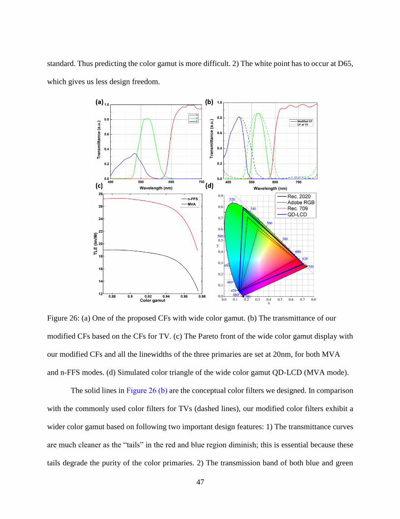
47

standard. Thus predicting the color gamut is more difficult. 2) The white point has to occur at D65,

which gives us less design freedom.

Figure 26: (a) One of the proposed CFs with wide color gamut. (b) The transmittance of our

modified CFs based on the CFs for TV. (c) The Pareto front of the wide color gamut display with

our modified CFs and all the linewidths of the three primaries are set at 20nm, for both MVA

and n-FFS modes. (d) Simulated color triangle of the wide color gamut QD-LCD (MVA mode).

The solid lines in Figure 26 (b) are the conceptual color filters we designed. In comparison

with the commonly used color filters for TVs (dashed lines), our modified color filters exhibit a

wider color gamut based on following two important design features: 1) The transmittance curves

are much cleaner as the “tails” in the red and blue region diminish; this is essential because these

tails degrade the purity of the color primaries. 2) The transmission band of both blue and green

48

color filters is narrowed to minimize the overlapping between different color channels. Figure 26

(c) depicts the Pareto Front for MVA and n-FFS modes. With the proposed color filters and setting

the linewidths of all three primary colors to 20nm, we can achieve ~97.6% of the Rec. 2020 color

gamut in CIE 1931, or ~98.6% in CIE 1976. The TLE of MVA is ~40% lower than that of n-FFS.

Such a wide color gamut display can reproduce most of the colors that Rec. 2020 demands [94].

If we inspect the color triangle in Figure 26 (d), we can determine that the color triangle overlaps

well with the Rec. 2020 standard except that the green deviates slightly. Table 4 lists the optimized

parameters for both MVA and n-FFS.

Table 4: System parameters of the widest color gamut we can get with the modified color filters,

for both MVA and n-FFS modes.

LC mode MVA n-FFS

Red 637.8 638.3

Green 530.9 530.5

Blue 469.1 467.6

TLE (lm/W) 12.1 18.3


If we compare Table 2-4, we can find the tradeoff between color gamut and TLE is quite

significant. For example, for the n-FFS mode shown in Table 2 and Table 4, when the color gamut

widens from 92.3% to 97.5%, which is 5.6% increase, the TLE drops from 24.6 to 18.3, which is

25.6% decrease in optical efficiency. Such a sacrifice may not be worth taking because power

efficiency is a critical issue for all displays. For practical applications, we need to balance color

gamut with optical efficiency. We will give a more detailed discussion in a later section.

49

Meanwhile if we compare the optimized wavelengths in Table 4 to those listed in [95],

which are optimized to cover the Pointer’s Gamut, we find that these two results are quite close

except for the green primaries. This similarity comes from the fact that Rec. 2020 is also designed

to cover the Pointer’s Gamut. As for the green primaries, they are a little bit different because of

the greatly modified green color filter in our design.

4.3 Wide color gamut RGB QLED

QLED has long been considered as a potential candidate for next generation display

because it offers narrow linewidth and selectable central wavelength. Moreover, the device

structure is similar to that of contemporary OLED. Consequently, QLED is also suitable for

flexible displays and its manufacturing is compatible to OLED. Previously, QLEDs are regarded

as a future technology because of its relatively low external quantum efficiency (EQE) and

relatively short lifetime. Recently, with the demonstration of high EQE and long life quantum dots,

there is renewed strong interest on QLED. Figure 27 (a) shows the typical device structures of high

efficiency RGB QLEDs. These structures are similar to those proposed in [82]. The efficiency and

emission spectra of the RGB QLEDs can be calculated by the dipole model [31, 96, 97] and the

simulation results agree well with experiments. If we assume that quantum efficiency and the

charge balance is unity, the corresponding EQE for the RGB QLEDs are 17.2%, 16.5% and 17.7%,

respectively. These results are quite close to the reported experimental data. In addition, if we

know the real quantum efficiency and charge balance of the device, we can get a better match

between simulation and experiment. The calculated normalized emission spectra of the RGB

QLEDs are shown in Figure 27 (b).

50

Figure 27: (a) Device structures and (b) emission spectra of the RGB QLEDs.

From Figure 27 (b) we find that the emission spectrum of each QLED fits well with the

Gaussian distribution; the R2 values for all three curves are all larger than 99.7%. Here the RGB

QLEDs shown in Figure 27 can realize 85% of Rec. 2020, which is still insufficient. We can still

optimize the color gamut coverage and LER simultaneously for the QLED. Results are shown in

Figure 28. The linewidths of the RGB QLEDs are 1) 30nm for RGB (blue curve; lower limit), 2)

30nm for red and green, and 20nm for blue (green curve, intermediate case), and 3) 20nm for RGB

(red curve; upper limit). As expected, the green curve lies between the red and the blue curves.

51

Figure 28: The relationship between color gamut and LER for RGB QLEDs.

From Figure 28, similar to QD-LCD, we cannot achieve 100% Rec. 2020 (ideal case)

because of the linewidth of the RGB QLEDs. However, RGB QLEDs can easily achieve 95% of

the Rec. 2020 standards even with a linewidth of 30nm because there is no crosstalk coming from

color filters. If we compare the blue and red curves, we can easily find that at the same color gamut

the LER is 13% higher for the QDs with 20nm linewidth. This suggests that for the EL case,

developing QDs with a reasonably narrow linewidth (~20nm) is advantageous for both color gamut

and efficiency. From Figure 28, we can find the following best result that RGB QLEDs can get:

when the central wavelength of the 20nm-linewidth RGB QLEDs is 634.3nm, 530.6nm and

465.8nm, respectively, we can get an optimized 98.4% color gamut (99.0% in CIE 1976) with a

high LER of 252.8 lm/W. Such a wide color gamut can be regarded as ready to reproduce most of

the colors that Rec. 2020 enables [94]. Compared to the ideal display (100% Rec. 2020 color gamut

with three monochromatic light sources), the LER of our RGB QLED is still 7.7% lower. If we

52

plot the color triangle in the CIE 1931 color space in Figure 29, we can easily catch that the red

and blue colors are quite close to the Rec. 2020 color primaries while the green color is still a little

bit off. Similar to QD-enhanced LCD, if we can squeeze the linewidth of the RGB QLEDs to 10nm,

then we can realize 99.5% of the Rec. 2020 color gamut with LER=251.5 lm/W. However, it

remains technically challenging to develop 10-nm-linewidth QDs.

Figure 29: The Color gamut representation of the proposed RGB QLEDs.

4.4 Discussions

Before we dive into the discussions about quantum dots for Rec. 2020 color gamut. We

would like to talk about some general concerns about wide color gamut displays. The first concern

is about observer metamerism [98, 99]: namely, different observers will see the same color

differently, especially for saturated colors. The other concern is that without proper color

management, quite a few colors will appear strangely on a wide color gamut display, for example,

skintone. While I agree that these concerns are reasonable, the hardware itself is not to blame. And

53

it is possible to mitigate these problems by multi-primary displays and better color management

[98, 99]. It will be fun when the color scientists and hardware engineers work together to deal with

these problems.

4.4.1 Color Space selection

As we have briefly mentioned before, the selection of color space for calculating color

gamut is quite important but sometimes misleading. For example, considering the RGB QLEDs

shown in Figure 27, the color gamuts in the CIE1931 and CIE1976 color space shown in Figure

30 (a)-(b) are 84.6% and 85.4%, respectively. The spectra of the RGB QLED are shown in Fig.

Figure 30 (c) and the LER of the RGB QLED display is 290.8 lm/W. From Figure 30 (a)-(b), we

can find that even though statistically speaking the color gamut in CIE 1931 and CIE 1976 is quite

similar, the visual feeling is quite different. In Figure 30 (a), it seems that the QLEDs can well

reproduce both red and blue, but not green. However, in CIE 1976 Chromaticity Diagram it seems

that the QLED can better reproduce green than red and blue. To answer which representation is

closer to reality, we convert the Rec. 2020 standard and the QLED color gamut to the CIELAB

color space, and the results viewed down from the L axis is shown in Figure 30 (d). The wireframe

color gamut is the Rec. 2020 standard and the solid color gamut is the color gamut of the QLED

display, we can intuitively determine that the maximum mismatch happens in the green color. This

suggests the color gamut shown in CIE 1931 color space is more correlated to the 3D color

perspective model, which matches the conclusion stated in [24]. Under this consideration, we

decide to calculate color gamut in CIE 1931. For real products, we have to analyze the color

difference of the display quantitatively and further calculate the volume-coverage ratio.

54

Figure 30: Color gamut of a RGB QLED in (a) CIE 1931 and (b) CIE 1976; (c) emission spectra

of the RGB QLEDs and (d) color gamut comparison of Rec. 2020 and the QLED display in CIE

LAB, the wireframe color gamut is Rec. 2020 and the solid color gamut is the RGB QLED.

4.4.2 Angular performance of QD-LCD and RGB QLEDs.

Color shift at an off-axis angle is a critical issue. For a QD-LCD, the angular performance

is primarily determined by the birefringence of the LC material [100]. Here we demonstrate that

with two wide-view LC modes: 1) two-domain (2D) n-FFS for smart phones and 2) 4D MVA for

TVs. From Figure 31 (a)-(b), the color shift of each RGB primary color is rather small and the blue

has the largest color shift. For the worst scenario, the color shift (Δu’v’) of the blue color stays

below 0.01 at 80° viewing angle. Such an LCD has negligible color shift. However, the color shift

for the white color is much larger. For the 2D n-FFS mode, the color shift is still smaller than 0.02

55

at 80° for RGB and white. The situation for 4D MVA is drastically different. For the white color,

the color shift is approaching 0.04 at 80° viewing angle. The small color shift for the RGB

primaries means that we do not have to worry about the color gamut shrink at large viewing angle.

While the small color shift for the white color in 2D n-FFS indicates that we can avoid the usage

of color mixing films [101] The reason that 4D MVA has a larger color shift than 2D n-FFS is that

for 4D MVA the LC directors are vertically tilted, while for 2D n-FFS the LC directors are rotated

in plane. In the former case, it is easier to observe the birefringence effect at off-axis. In

commercial TV products, 8D MVA is commonly used to mitigate the color shift [90].

Figure 31: (a) Color shift of QD-LCDs for 2D n-FFS and 4D MVA, and (b) the normalized

output spectra of the QD-LCD at different viewing angle.

As for the RGB QLEDs, color shift comes from cavity effect [102], The angular

performance of RGB QLED can also be evaluated by the dipole model. For example, for the RGB

QLED mentioned in Figure 27, the angular dependent emission spectra are shown in Figure 32 (a)

and we can find that each individual spectrum remains quite narrow even at a large off-axis angle.

From Figure 32 (b), the color shift of each individual color R, G and B is quite small. The largest

color shift Δu’v’ for blue is still smaller than 0.002, which is quite small. As for the combined

56

white color, Δu’v’ reaches 0.02 at 65°. The reason for the relatively large color shift for the white

color can be deduced from Equation (13) and Figure 32 (a). As demonstrated in Equation (13), the

white color is optimized for the normal viewing angle. For the off-axis angle, the emission pattern

drops differently for different colors, thus Equation (13) no longer matches the system’s white

point. To reduce color shift, we can optimize the QLED cavities to tune the angular emission

pattern. However, this approach is quite unintuitive and it is difficult to predict how the angular

emission pattern changes with different QLED stack configuration. Another way is to use optical

diffusers, microstructures or other kinds of color mixing films to mitigate the color shift. This

approach has been widely used in contemporary LCDs [101].

Figure 32: (a) Angular dependent emission spectra for the RGB QLED; and (b) Color Shift of

the RGB QLEDs.

4.4.3 Comparing QD-LCD with red and green phosphors embedded LCD

Besides QDs, two-phosphor LEDs (2p-LED, i.e. blue LED pumping red and green

phosphors) have also attracted much attention because of their excellent reliability and low cost.

Figure 33 (a) shows the emission spectra of such a 2p-LED [77, 103]. From Figure 33 (a), the

green and red emission spectra are relatively broad as compared to quantum dots. Our simulation

57

results in Figure 33 (b) show that for this 2p-LED backlit LCD system with the color filters

designed for TV, it covers 90% of the Adobe RGB and 67% of the Rec. 2020, and the TLE is 21.7

lm/W for the n-FFS mode and 15.6 lm/W for the MVA mode. Therefore, we find that theoretically

QD offers wider color gamut and higher optical efficiency than 2p-LED. However, contemporary

red and green phosphors can be deposited on top of the blue LED chip to form a white LED [104].

whereas for red and green QDs, it is still not mature to place them on the blue LED chip [105]

because of the material reliability issue. The “on edge” and “film” approaches for QDs are not as

efficient as the white LED with 2p phosphors because of the longer optical path.

Figure 33: (a) The spectra of the RG phosphor embedded LCD and (b) its color triangle.

Recently, the red KSF phosphor [106] became the star for the display industry because of

its deep saturated colors. Combining blue LED with red KSF phosphor and another green phosphor

has become the standard approach for wide color gamut displays nowadays. While this

configuration has no problem achieving the DCI-P3 color gamut, it is still inferior to QDs in terms

of Rec. 2020, especially for the green color. At the same time, this new 2p-LED lacks the flexibility

of the QD approach.

58

4.5 Summary

Wide color gamut is another import feature of HDR displays. We have analyzed how to

obtain a wide color gamut display for both QD-LCD and RGB QLEDs. The relationship between

optical efficiency and color gamut is explained for both approaches. For QD-LCDs, we can easily

achieve more than 90% of the Rec. 2020 standard through spectral optimization with contemporary

commercial color filters. However, to realize more than 97% of Rec. 2020, color filters have to be

modified and TLE sacrificed. The angular performance of QD-LCDs is determined by the LC

mode. With 2D n-FFS mode, the combined white color exhibits an indistinguishable color shift.

As for RGB QLEDs, it can easily achieve Rec. 2020 through spectral optimization, and the angular

performance of the QLEDs is mainly governed by the QLED cavity. For each primary color, the

color shift is negligible; but for the combined white color, the color shift might still be noticeable.

This knowledge can be used to design wide color gamut HDR displays.

59

CHAPTER FIVE: ACHIEVING 12-BIT PERCEPTUAL QUANTIZER

CURVE FOR HIGH DYNAMIC RANGE DISPLAY

For HDR displays, we need more bit-depth to accommodate for the enlarged luminance

range [18, 107]. Analysis of the human contrast sensitivity function indicates that the traditional

8-bit gamma encoding is no longer suitable for HDR content. Because of this, new electoral-optical

transfer functions (EOTFs) have been proposed to replace the 8-bit gamma encoding. Among them,

the most important ones are the hybrid log-gamma (HLG) encoding and the perceptual quantizer

(PQ) curve [30]. The PQ encoding is also known as the ST.2084 standard. While both curves have

been widely used, the HLG encoding is only intended for live production. Generally, it is believed

that the 12-bit PQ curve covering 0-10,000 nits should be an ultimate goal for the display industry,

as it guarantees no visual banding between adjacent grey levels.

Two display technologies could be implemented as HDR displays. The first one is OLED,

which is possible to achieve perfect pitch black. However, because of the material lifetime concern,

its peak brightness is usually below 1000 nits. The second approach is to use dimmable LED arrays

as LCD backlight to dynamically control the dark state of the device. Currently, the peak brightness

of LCD using local dimming backlight can achieve 4000 nits. With the emergence of high

brightness LEDs, it is possible to achieve 10,000 nits in the near future. Therefore, achieving 12-

bit PQ curve will become more and more critical for the display system. In this thesis, we will

focus on the local dimming LCD approach. Finally, the author would like to mention that for

cinema systems, there is a different criteria to be certificated as HDR. The main difference

60

5.1 Achieving 12-bit PQ curve: Driving the LC and LED separately

Figure 34 illustrates the 12-bit PQ curve together with a 12-bit gamma 2.2 curve. The

detailed equation for describing the PQ curve can be found in [30]. From Figure 34 we can see

that compared with the traditional gamma curve, the PQ curve increases much more slowly. In

addition, there are ~2000 gray levels in the low luminance range (i.e. 0-100 nits). This ensures that

the PQ curve is compatible with contemporary SDR standards. Assuming the peak brightness of

the system is L and the contrast ratio of the LC panel is C, then the minimum brightness of the

LCD without local dimming is L/C. This gives us an intuitive and straightforward driving method

for the local dimming system:

1) For the luminance between L/C and L, the LED backlight is working at full

brightness and we could control the LC panel to get the required luminance range.

2) For the luminance under L/C, the LC is turned to off state whereas the LED is

dimmed to achieve the target luminance range.

Figure 34: The 12-bit ST-2084 curve displayed together with the 12-bit gamma 2.2 curve.

61

Throughout this thesis, we assume the system peak brightness L is 10,000 nits. As for the

LC part, we decide to use the vertical alignment (VA) mode [108] because of its high contrast ratio.

Considering the capability of current TFT technology, we set the voltage interval between two

adjacent gray level is around 5 mV, thus for a 12-bit display, the voltage swing (ΔV = Von – Vth)

should be ~20 V. To achieve this ΔV, in experiment we mixed a negative dielectric anisotropy (Δε

< 0) LC material ZOC-7033 (JNC, Japan) [109] with a positive Δε LC material MLC-6686

(Merck). The recipes for the new LC mixture are listed in Table 5. The obtained new LC mixture

exhibits a small, but negative dielectric anisotropy (Δε = -0.89), thus a large voltage swing (ΔV

~20 V) can be achieved.

Table 5: Recipe for the new LC mixture.

Component ratio Δn Δε

ZOC-7003 75.2% 0.103 -4.36

MLC-6686 24.8% 0.0983 10.00

Next, we filled this new LC mixture into a commercial VA test cell with cell gap d = 3.3μm.

Figure 35 shows the measured voltage-transmittance (VT) curve of the mixture, in which the

threshold voltage Vth is 11.12V and on-state voltage Von≈30V. The measured contrast ratio of the

LC cell is ~5000:1. This indicates that driving the LC alone we can get 2 nits to 10000 nits; below

2 nits we need to dim the LEDs to achieve the target luminance.

62

Figure 35: Measured VT curve of the LC cell: d=3.3 µm and λ=633 nm.

To analyze the performance of the LC cell, we selected 24 gray levels based on the 12-bit

PQ-curve. The 24 gray levels are listed in Table 6.

Table 6: The selected 24 gray levels.

Gray level Luminance (nits)

Corresponding

transmittance (%)

Gray level Luminance (nits)

Corresponding

transmittance (%)

771 2.002 0.020 2303 170.274 1.703

865 2.904 0.029 2462 246.848 2.468

965 4.197 0.042 2623 357.454 3.575

1073 6.090 0.061 2785 516.542 5.165

1187 8.817 0.088 2950 749.196 7.492

1307 12.747 0.127 3115 1084.617 10.846

1434 18.473 0.185 3280 1569.166 15.692

1566 26.705 0.267 3446 2276.360 22.764

1705 38.762 0.388 3610 3292.626 32.926

1848 56.101 0.561 3773 4764.176 47.642

1996 81.278 0.813 3935 6902.473 69.025

2148 117.722 1.177 4095 10000.000 100.000

63

As discussed above, ~50% gray levels are in the low luminance region. For such a low

transmittance, the driving voltage would be quite close to the threshold voltage; therefore, the

response time would be slow [110]. To confirm this, we measured the gray-to-gray (GTG)

response time between these twenty-four gray levels, and results are tabulated in Table 7. The

average GTG rise time of the LC cell is 33 ms, which is too sluggish for practical applications.

This indicates driving the LC and the LED separately is not suitable for the 12-bit display.

Table 7: The gray-to-gray response time of the LC cell between the selected 24 gray levels.

(Unit: ms)

1 2 3 4 5 6 7 8 9 10 11 12 13 14 15 16 17 18 19 20 21 22 23 24

1 123.6 120.8 116.4 111.7 106.3 93.0 89.1 83.1 79.2 72.3 66.2 60.3 54.1 40.3 39.7 36.1 32.4 29.3 26.9 17.4 13.0 8.0 2.5

2 2.5 105.0 96.6 86.0 76.4 76.2 72.5 68.8 67.4 62.4 58.2 52.6 48.9 43.7 38.6 32.7 29.1 25.0 20.3 15.7 11.8 7.7 2.4

3 2.6 88.8 95.8 89.4 85.2 79.8 75.0 71.3 66.4 62.6 58.3 53.4 49.1 41.9 38.8 35.1 28.9 23.9 19.6 15.7 11.6 7.7 2.4

4 2.6 85.8 95.2 78.7 76.0 74.3 74.1 69.6 67.8 62.8 58.8 54.1 49.2 41.4 40.9 32.6 28.6 24.5 19.8 15.7 11.6 7.6 2.4

5 2.6 83.2 76.0 84.6 76.8 74.4 72.1 70.6 69.1 64.2 58.0 53.0 48.2 41.6 40.3 32.9 28.4 24.2 19.8 15.4 11.5 7.5 2.4

6 2.6 80.2 78.4 80.2 80.3 73.8 68.4 67.7 66.6 60.5 57.3 52.3 48.1 41.0 37.5 35.4 28.2 23.9 19.3 15.5 11.4 7.5 2.4

7 2.7 73.1 71.7 75.3 70.7 71.9 67.8 61.2 60.3 59.4 54.0 49.8 47.2 40.1 35.0 33.7 28.2 23.2 19.6 15.3 11.6 7.6 2.4

8 2.7 68.5 69.5 73.0 70.3 71.9 66.0 63.0 60.0 57.6 53.7 48.8 45.1 40.6 34.7 33.1 28.5 22.3 18.8 14.7 11.3 7.4 2.4

9 2.8 66.3 67.4 68.6 68.6 68.2 61.1 59.3 58.2 55.3 50.8 48.0 43.8 40.0 36.7 31.3 26.5 23.0 18.4 14.9 11.1 7.4 2.4

10 2.8 62.7 64.0 63.8 63.8 63.3 60.2 58.7 57.1 54.2 50.8 47.0 42.7 40.6 37.0 31.0 26.7 22.1 18.2 14.5 11.0 7.3 2.3

11 2.8 58.4 59.2 58.5 57.9 58.0 57.1 55.4 56.7 57.3 48.6 43.8 40.2 34.1 33.7 28.8 25.7 22.3 17.5 14.4 10.9 7.1 2.3

12 2.9 54.7 54.8 55.2 55.8 54.6 52.1 52.1 51.6 48.4 49.7 42.0 39.7 35.9 33.1 29.9 25.9 21.5 18.0 14.3 10.6 7.1 2.3

13 2.8 50.1 51.1 50.7 50.5 50.5 49.3 47.6 47.5 45.4 43.9 42.5 39.0 32.3 30.4 26.2 23.6 21.1 17.3 13.6 10.4 6.9 2.2

14 2.9 46.1 46.5 46.5 46.4 46.0 45.9 44.6 44.0 43.4 42.2 41.6 38.1 32.2 33.7 26.3 24.4 19.7 17.0 13.8 10.3 6.8 2.2

15 3.0 43.4 39.2 42.2 41.5 42.2 45.2 44.0 44.3 38.6 39.6 39.4 39.3 34.9 31.7 27.9 22.8 19.2 16.2 13.4 9.9 6.6 2.2

16 3.1 39.4 37.2 40.6 40.2 37.3 37.2 39.5 38.2 37.9 35.7 32.5 31.4 33.0 28.0 27.0 21.7 19.5 15.6 12.5 9.9 6.5 2.2

17 3.2 35.7 36.9 35.2 33.5 36.5 36.2 38.5 37.2 33.9 32.2 32.5 29.3 30.7 26.9 29.0 24.4 17.4 15.4 12.7 9.3 6.3 2.1

18 3.4 33.5 31.4 31.3 31.2 31.1 31.6 34.2 33.0 30.8 30.0 31.1 30.5 29.0 26.5 23.7 21.8 18.2 14.8 12.2 9.1 6.2 2.1

19 3.6 30.2 27.8 29.3 29.0 29.2 28.7 27.9 29.1 27.6 28.7 27.8 26.0 25.9 25.3 24.2 21.2 19.2 15.6 12.0 8.7 6.2 2.0

20 3.7 25.9 25.5 27.0 26.9 26.5 26.0 27.3 27.3 26.0 25.4 26.0 24.1 24.4 23.0 21.6 20.2 19.0 16.6 10.8 8.6 5.7 2.0

21 3.9 23.8 23.1 24.1 24.1 23.9 23.9 23.3 24.6 23.8 23.2 23.8 23.0 22.7 21.3 20.5 19.2 16.6 15.6 14.2 8.7 5.8 1.9

22 4.1 20.7 20.9 21.8 21.8 21.5 21.5 22.1 21.7 21.7 22.2 21.9 21.9 21.2 19.7 19.1 17.8 16.2 14.8 12.9 10.4 5.8 1.9

23 4.4 18.2 19.0 19.7 19.7 19.6 20.1 20.3 20.2 20.4 20.2 20.4 20.3 19.8 19.2 18.1 17.2 15.5 13.9 12.1 10.2 8.0 1.7

24 4.9 16.5 17.0 17.3 17.5 17.3 17.9 17.9 18.1 18.2 18.1 18.1 18.1 17.9 17.7 16.6 16.2 14.8 13.4 11.6 9.8 7.9 5.5

64

5.2 Achieving 12-bit PQ curve: Driving the LC and LED simultaneously

As analyzed above, driving the LC panel or the backlight LEDs alone is not suitable for

achieving the 12-bit PQ curve. Thus, we need to drive the LC and the LEDs simultaneously. The

most intuitive approach can be explained by Equation (15):

1 2 1 2, ) ( ) ( )( .G L G T GL G (15)

Here, G1 and G2 represent the gray level of the LED and the LC, respectively, L is the

luminance of the system, and T is the transmittance of the LC. By controlling the gray level of the

LC and the LED simultaneously, it is possible to achieve 12-bit PQ curve. Assuming the LEDs

and the LC panel have S1 and S2 gray levels, respectively, in theory the system will have S1×S2

gray levels. An example is that the LEDs are 4-bits (16 gray levels) and the LC panel is 8-bit (256

gray levels).

The abovementioned approach is quite straightforward; however, a severe flaw of this

approach is that the same luminance may be achieved by different gray level combinations. This

reduces the overall gray levels of the system. At the same time, without careful gray level selection,

this approach will introduce severe image noises. This can be explained by the following thought

experiment: the display is required to show two adjacent achromatic pixels and the target

luminance for the two pixels are 100 and 93.88 nits, respectively. Assuming the LC panel follows

the 8-bit gamma 2.2 curve, at least two possible gray level combinations can achieve the targets:

1) For both pixels, the LEDs work at 100 nits, and the LC works at gray level 255 for

the first pixel and gray level 248 for the second pixel. The actual luminance for the two pixels are

100 and 94.06 nits, respectively.

65

2) For the first pixel, the LED works at 100 nits and the LC works at gray level 255;

for the second pixel, the LED works at 1000 nits whereas the LC works at gray level 87. The actual

luminance for the two pixels are 100 nits and 93.88 nits, respectively.

At first glance, the two combinations seem identical and the second combinations seems

even closer to the target luminance. However, in real applications the first combination is superior

to the second one. The first reason is that in local dimming LCDs, most of the time it is not possible

to do pixelated local dimming [1, 19, 49], thus, the two pixels might belong to the same section

where only one LED is available. The second reason is that even if it is possible to do pixelated

local dimming, because of the point spread effect [1], there will be crosstalk between the adjacent

pixels, and the second configuration will introduce salt-and-pepper noises [111] to the displayed

image. In this sense, a driving scheme where there is no sudden jump in gray level combinations

is preferred. Based on this requirement, we propose a new driving scheme with the following steps:

1) Predetermine a tone response curve Li of the LEDs, here L is the luminance and i=0,

1, 2,.., N1-1 is the (i+1)-th gray level. In total, there are N1 grey levels.

2) For the target luminance Lt that satisfies Li≤ Lt< Li+1, the gray level of the LED for

this target is set to i+1.

3) Determine the corresponding LC transmittance Tj based on Equation (15). After

calculating all the LC transmittance for all the target luminance, it becomes possible to construct

the tone response curve Tj of the LC panel. Here j is the (j+1)-th gray level of the LC panel. In

total there are N2 gray levels.

4) Optimizing the tone response curve Li and Tj according to the device limit and the

12-bit PQ curve.

66

With the abovementioned approach, we can ensure that one target luminance corresponds

to a single gray level combination, and the gray level combinations will change smoothly if

properly designed. Based on this approach, we designed the tone response curve of the LEDs and

the LC by comparing with the 12-bit PQ curve. The tone response curves for the LEDs and the LC

are shown in Figure 36 (a)-(b), respectively. Here we have 57 gray levels for the LEDs and 256

gray levels for the LC. When they are combined together, the final tone response curve is shown

in Figure 36 (c) and it is clear that this curve matches well with the 12-bit PQ curve.

Figure 36: Tone response curves of (a) the LEDs, (b) the LC panel and (c) the whole system in

comparison with the target 12-bit PQ curve.

To quantify the difference between the actual tone response curve M and the 12-bit PQ

curve R, we calculated the coefficient of variation (CV) [112] between the two curves, and the

definition of CV is:

67

1

0

2( )100%

.i i

N

M R

CVNR

(16)

Here N is the total gray levels and R is the average luminance of the PQ curve. As can be

seen from Equation (16), the CV describes the agreement between the two data sets. The calculated

CV here is 0.08%, which indicates with our proposed tone response curves shown in Figure 36,

the system can well reproduce the 12-bit PQ curve.

In the previous section, we have mentioned that if we drive the LEDs or the LC separately,

the LC panel will have sluggish response time and high on state voltage. For our driving scheme

proposed above, the response time and driving voltage of the LC panel is no longer a problem as

the panel is still 8-bit except that the tone response curve is different. To prove this, we made a

3.3μm-cell-gap VA cell with ZOC-7003. The V-T curve of the cell is shown in Figure 37. The on-

stage voltage of the cell is 7.5V with a threshold voltage of 2.25V. Such driving voltage is typical

for commercial LCD systems.

Figure 37: The voltage-transmittance curve of VA cell using ZOC-7003.

68

As for the response time, the transmittance curve is equally divided into 8 gray levels and

the measured GTG response times [63, 64] are shown in Table 8. The average response time of

the cell is 6.17 ms. Such response time is fast enough for real applications.

Table 8: Gray-to-gray (GTG) response time of the ZOC-7003 VA cell. (ms)

Gray

levels

1 2 3 4 5 6 7 8

1 17.01 12.51 10.01 8.2 6.04 3.07 1.1

2 2.85 11.25 9.19 7.07 4.87 2.82 0.97

3 3.34 12.15 8.3 6.43 4.66 2.64 0.88

4 3.65 11.82 9.61 6.09 4.39 2.51 0.83

5 3.97 11.39 9.46 8.45 4.44 2.41 0.8

6 4.31 11.04 9.41 7.81 6.19 2.4 0.79

7 4.71 10.44 9.3 7.79 6.17 4.58 0.69

8 5.15 10.55 8.96 7.51 5.86 4.21 2.2

69

5.3 Summary

We have proposed an approach that drives the local dimming LED backlight and LC panel

simultaneously to achieve the 12-bit PQ curve for HDR displays. Compared to driving the LEDs

and LC panel separately, this approach exhibits fast response time and acceptable driving voltages.

At the same time, our approach will not introduce imaging noise to the system.

Besides driving the LEDs and the LC panel together, another possible way to achieve the

12-bit PQ curve is to use the dual LC panel approach, which we have already talked about in

Chapter 2. In this approach two LC panels are driven together to achieve increased bit-depth and

darker black state. One common difficulty for these two approaches is the synchronization: for the

first approach, the synchronization between the LEDs and the LC will be the main challenge

whereas for the second approach synchronizing the two LC panels will be a burden for the circuit

design. Besides this challenge, each approach has its unique pros and cons. For the first approach,

designing the LED backlight will be quite challenging, as we have to consider the point spread

function of the LEDs, also, the backlight design will be even more complex if we would like to

use edge-lit LEDs instead of direct-lit LEDs [113]. For the second approach, the added LC panel

reduces the overall optical efficiency and increases the thickness of the system. In the author’s

opinion, these two approaches would co-exist for different requirements and user scenarios.

70

CHAPTER SIX: REPRODUCING HIGH DYNAMIC RANGE CONTENTS

BASED ON DISPLAY SPECIFICATIONS

As we have mentioned in the introductory chapter, besides the hardware limit, current

display pipelines treat the HDR contents incorrectly, which result in image rendering that violates

the content creator’s intension. At the same type, because of the manufacturing tolerances, even

the same batch of displays might have different white point, peak brightness and dark state. That

is why we want to improve the display pipelines to reproduce the HDR contents adaptively based

on display configurations.

Before we dive into the topic, we would like to mention that there are two kinds of HDR

content: HDR images and HDR videos. The difference between these two are that most of the time

HDR images do not come with absolute luminance info whereas professional color graded HDR

videos contain absolute luminance info via the PQ encoding. In our analysis, we will only talk

about professionally graded HDR video footage.

6.1 Reproducing HDR content via HDR gamut mapping

As is mentioned above, standard display pipeline cannot faithfully reproduce HDR content.

Displaying HDR content on all kinds of media is actually not new topic and there are many tone

mapping approaches around to deal with this problem, for example, the iCAM06 image appearance

model [16] and the photographic tone mapping approach [114]. These algorithms work quite well

in terms of HDR imaging. However, they are not suitable for displaying HDR videos in real time:

the fast-bilateral spatial filtering used in iCAM06 consumes too much processing power. In the

photographic tone mapping approach, calculating the average luminance of each frame is quite

challenging if we would like to display 4K HDR video in real time. In this sense, a color-by-color

71

solution is preferred as it can be constructed as a color look up table (CLUT) and incorporated into

silicon, such as the graphics hardware or the display timing controller. This motivates us to develop

a new color-by-color reproduction approach to display HDR content. Before we talk about our

approach, we would like to look at how contemporary TVs interpret HDR content, which is shown

in Figure 38 (a). After decoding the content to RGB values, the contents are first gamut mapped

and then tone mapped [115] before finally being displayed on HDR/SDR display. For content

encoded with Dolby Vision, this process can be done with the dynamic metadata [116]. However,

for content encoded with HDR10, this process is dependent on the TV manufactures. In our

approach, we combine the two processes together by manipulating the lightness and chroma

simultaneously through HDR gamut mapping, as is demonstrated in Figure 38 (b).

Figure 38: (a) Display pipeline for HDR contents on contemporary TV and (b) the proposed

HDR gamut mapping algorithm.

The detailed approach of the HDR gamut mapping is explained below:

1) Determine the reference white. The reference white we select has absolute XYZ

value of (76.0374, 80.0000, 87.1176). This white point is selected based on the content metadata,

sRGB standard [117] and the fact that most displays have D65 white point. We’ll talk more about

reference white selection in the discussion part.

72

2) Select the working color space. Here we select the IPT color space [118] because

of its simplicity and hue linearity. The IPT color space is extended to beyond unity to allow for

RGB values larger than one.

3) Construct the color gamut of an ideal wide color gamut HDR display. Here we

assume the original display is an HDR display with a peak brightness of 1200 nits and is fully

capable of displaying BT. 2020. All the colors it can reproduce is converted to the IPT color space.

Color space selection will be explained in more details later in this chapter.

4) Construct the color gamut of the real SDR display. The target display here is with

peak brightness of 400 nits and sRGB color gamut. Similarly, all the colors it can reproduce is

converted to the extended IPT color space.

5) Gamut mapping from the original color gamut to the destination color gamut. The

approach we use here will be explained later. Of course, content creators can opt for other gamut

mapping approaches.

6) Transform the gamut-mapped content back to display RGBs.

The color gamut of both the HDR and the SDR display is demonstrated in Figure 39 (a)

and the general working principle of the HDR gamut mapping approach is depicted in Figure 39

(b). Basically this approach scales lightness and chroma on a constant hue plane. The advantages

of this approach are threefold: 1) This color-by-color reproduction approach is relatively easy to

incorporate it into the hardware level as a 3D CLUT; 2) This approach is display adaptive. For

example, if the peak brightness of the SDR display is 600 nits, we just need to reconstruct the

destination color gamut, do gamut mapping again and create another 3D CLUT; 3) it is flexible

enough to incorporate color preference.

73

Figure 39: (a) the color gamut of both the HDR display and the SDR display and (b) the principle

of the HDR gamut mapping approach.

The first step of the gamut mapping approach is the lightness mapping. The lightness

mapping curve is shown in Figure 40. Here we use Io and It to denote the peak lightness value of

the original display gamut and the target display gamut, respectively. The mapping curve is

designed based on these two principles: 1. For lightness values between 0 to 1, which corresponds

to luminance between 0 and 80 nits, there is no lightness distortion. In this way contents with

luminance level up to the reference white can be well preserved. 2. For lightness values larger

than unity, they are mapped through a Bézier curve with control points (1,1), (Io,Io) and (It, Io).

With this step the highlights can be well preserved on the target display.

(a) (b)

74

Figure 40: lightness mapping curve used in our algorithm.

The second step of the algorithm is the chroma mapping along constant lightness. This step

is well documented in the BasicPhoto algorithm developed by Microsoft, which is a variant of the

chroma-dependent sigmoidal lightness mapping and cusp knee scaling (SGCK) approach [119].

However, for our gamut mapping approach we are using the IPT color space.

6.2 HDR display setup

To test the algorithm, we built an HDR display by combining a projector with an LC

module [18]. In this way we have formed a pixelated local dimming HDR display. The

specifications of the HDR display are listed in Table 9. With this HDR display it is possible to

both display HDR contents and simulate an SDR display.

75

Table 9: Specification of the HDR display.

Peak brightness 1160 nits

Dark State 0.002 nits

Contrast Ratio 580,000:1

Color gamut sRGB

Bit depth 12 bit

The device model of this dislpay can be described by the following equation [120]:

( ) ( ) ( ) ( )

( ) ( ) ( ) ( )

( ) ( ) ( )

( ) ( ) ( ) .

1 1( )

R G B K

R G B K

R G KB

S S S S

S S S S

S

R RX X X X X

G GY P S M S P S Y Y Y Y

B BZ Z Z Z ZS S S

(16)

Here S is the digital counts of the projector and P(S) describes the luminance attenuation

of the projector, the matrix M transforms linear RGB values to CIE XYZ values by taking into

consideration the light leakage of the panel. Note that M is also dependent on L because of the

primary shift [121] of the projector under low light level. With Equation (16), when we get the

XYZ value of the scene, it is possible to calculate a grayscale image for the projector and a color

image for the LC module, and when they superimpose together we are able to reconstruct the

original HDR scene. This process is demonstrated in Figure 41. This HDR image is from Dr. Mark

Fairchild’s HDR survey [2]. The gray level image and the color image are the actual image we

sent to the projector and the LC module respectively, whereas the final image is a tone mapped

version of the image through the iCAM06 image appearance model. Notice that this image is only

used as a demo, it is not used in our pschophysical experiment. At the same time, this photo is

different from common HDR images that this is a professional HDR image with absolute

76

luminance info. At the same time, this image is different from HDR videos that it uses a linear

encoding and does not specify its color gamut.

Figure 41: How HDR image is displayed on our HDR device.

6.3 The psychophysical experiment

Besides testing the algorithm, another reason we would like to set up this device is that

even though contemporary SDR displays are still inferior to the HDR displays, it is possible to

improve their performance to some extent. For example, the peak brightness of the SDR displays

can be improved by using high efficiency OLED panel/LED backlight. Thus we would like to

know how peak brightness and dark level will affect the performance of SDR display. For these

two purposes, we conducted a psychophysical experiment. The experiment was conducted as

follows:

We prepared eight HDR images and these images are listed in Fig. 8. The second image is

the same as Figure 4 whereas all the other HDR contents are from the HDR clip Colors of the

Journey and the images shown in Figure 42 are tone mapped versions of the original HDR frames

via highlight compression. For each HDR image, ten versions were created: The first version was

a gamut-mapped version from BT. 2020 to sRGB to accommodate the HDR display’s color gamut,

this version was still HDR. For the other nine versions, they were the SDR versions that had been

77

processed with the HDR gamut mapping. The difference between these images were that they

came with three different peak brightness settings: 400 nits, 640 nits and 800 nits. As for the dark

level, there were also three configurations:0.005 nits, 0.1 nits and 0.25 nits. Thus there were 10

versions in total. The psychophysical experiment was conducted through pair-wise comparison. A

randomly selected version from the set of the SDR images was displayed together with the HDR

image, and the viewers were asked to judge how similar these two images were based on five

categories: 1) overall brightness 2) details 3) colors 4) highlights and 5) dark shadows. Then they

gave a score between 0% (totally different) to 100% (identical) to describe the similarity between

the two images. The viewing condition was dark with ambient illuminance of 10 lux.

Figure 42: The eight HDR frames we have used in the psychophysical experiment; these images

are ton-mapped version of the original HDR scene.

This process is demonstrated in Figure 43. The top image is an SDR version with peak

brightness of 400 nits and dark level of 0.25 nits while the bottom image is the HDR version.

Figure 43 is taken directly from the HDR display and because of the camera limit, it is not identical

to what the viewers saw on the display. Still we can tell that the HDR version has brighter

highlights and better color saturation than the SDR version. However, comparing Figure 43 with

Figure 4 we can tell that our HDR gamut mapping approach can well reproduce the HDR content.

78

Figure 43: Comparing the SDR image with the HDR version.

After all 18 viewers gave their answers for all of the images, we analyzed the data and

found some important results. The first question we would like to ask is “black or white: which is

more important?” The reason we ask this question is that the two mainstream display technologies

have different challenges when dealing with HDR contents. For OLED the dark level can be

perfectly black, but because of the lifetime issue it is not recommended to make the peak luminance

too bright. On the other hand, for LCD the peak brightness can be extremely high by using high

power LEDs, whereas the dark state is usually not satisfying because of the light leakage. The first

conclusion is that dark level is as important as peak brightness. This can be seen from the results

for Figure 42, image (2) and (3), which is listed in Table 10. Here b stands for dark level and w

stands for peak brightness. For image 2 the average luminance of the scene is 220 nits and the sun

area is over 1000 nits. When we increase the peak brightness, the perceived similarity between the

SDR and the HDR image dramatically increased, whereas when we decrease the dark level, the

similarity did not improve much. In fact, if we calculate the correlation coefficient rb between dark

level and similarity score, the result is rb=-0.159, which indicates poor correlation. Whereas for

the relationship between peak brightness and similarity score, the correlation coefficient rw=0.954.

This indicates that for image (2), people care much more about the white level than the dark level.

79

As for image (3), the average luminance is only 0.38 nits and the night sky is intended to be pitch

black. This time in general decreasing the black level has greatly improved the similarity score

(rb=-0.886), whereas the peak brightness is poorly correlated with the image similarity with rw=-

0.024. This indicates for this image, even though the stars should be over 1000 nits, people are

much more sensitive to the black level because it is a night scene. For the other six images, the

trend is similar: when highlights dominate the image, the similarity scores are well correlated with

the peak brightness (Figure 42 (8)); and when the image is dominated by dark pixels, the similarity

is most determined by the lowest dark level (Figure 42 (1)). For the other four images, the

similarity is dependent on both the peak brightness and the dark level. Summarizing these results

together, we can see the influence of peak brightness and dark level is image dependent and to

cater to the entire different image types, the dark level and peak brightness should be improved

simultaneously.

Table 10: Similarity (in percentage) for Figure 42, image (2) (data on the left side) and (3) (data

on the right side).

b\w 400 640 800

b\w 400 640 800

0.005 55 61.31 68.13 0.005 67.81 72.63 70.19

0.1 56.25 61.44 63.63 0.1 70.88 70.31 69.63

0.25 52.19 61.19 65.31 0.25 60.63 60.81 57.88

When we look at the mean opinion score (MOS) for all the eight images, what we got is

listed in Table 11, from the table we can see that for the worst scenario, viewers still give a high

similarity score of 68.82%, which indicates our HDR gamut mapping approach works quite well.

A closer look at the data demonstrates that in general higher peak brightness and darker black level

improves the similarity. However, at 0.1 nits to 640 nits, people give a high similarity score of

75.05%, and the improvement after that is not that dramatic. From Table 11 we can tell that even

though it is not possible for an SDR display to look 100% like an HDR display. Improved peak

80

brightness and dark level, together with our HDR gamut-mapping algorithm, helps enabling better

viewing experience. At the same time, the viewing experience improvement is limited. Overall

speaking, when we reduce the dark level from 0.25 nits to 0.1 nits, there is a noticeable

improvement in similarity, however, when the dark level is reduced further to 0.005 nits, it is quite

challenging for the viewers to notice the improvement. This suggests that 0.1 nits can be regarded

as a minimum requirement for faithfully reproduce HDR content on an SDR display. As for the

peak brightness, the improvement from 400 nits to 640 nits results in a boost in similarity score,

whereas further boost the peak brightness to 800 nits can only mildly improvement the similarity.

This indicates that compared with the HDR display with peak brightness of 1160 nits, 400 nits

peak brightness is too “dim” and could not enable a visually appealing highlights representation.

Whereas the boost from 640 to 800 nits is not significant enough to make the latter more similar

to the original HDR scene. In the meantime, it is quite challenging to make an SDR display with

800 nits because of the high power consumption. These two reasons together suggest that 640 nits

can be regarded as another minimum requirement for an SDR display to faithfully represent the

HDR content. In summary, luminance range between 0.1 nits to 640 nits can be regarded as the

minimum range for displays to appear HDR-like.

Table 11 Mean opinion similarity score (in percentage). (in percentage)

b\w 400 640 800

0.005 71.92 75.92 76.70

0.1 72.41 75.05 76.98

0.25 68.82 73.98 75.5

81

6.4 Discussions

6.4.1 Reference point selection

In our approach, we select the reference white as 80 nits based on the sRGB specification

and the content metadata, and it is also plausible to map reference white to 100 nits based on the

Rec. 709 standard [69]. However, we would also like to ask ourselves: “what will happen if we

select reference white at higher luminance?” To answer this question, we did a comparison

assuming that the peak brightness of the SDR display is 400 nits, the results are show in Figure 44.

Figure 44 (a) is the simulated HDR gamut mapped image assuming the reference white is 80 nits

whereas for Figure 44 (b) the reference white is 300 nits. We can clearly tell that when we increase

luminance of the reference white, the overall image brightness is enhanced. However, we lose

local contrast in the highlight region. This is predictable as we have less luminance range to

compress the highlights. The extreme case has already been shown in Figure 4 where reference

white equals display white and all the highlights are clipped. In fact, if we look at ST-2084 standard

we can tell that the intention of HDR display is not to have contents with higher overall image

brightness, but to have more room faithfully reproducing the highlights. Because of this intention,

the average pixel level (APL) of an HDR display should be similar to an SDR display and the

reference white should also be similar to contemporary TVs, which is around 100 nits. In this sense,

mapping reference white to luminance range larger than 100 nits might violate the content creators’

intention.

82

Figure 44: HDR gamut mapped versions of Figure 42 (5) with reference white of (a) 80 nits and

(b) 300 nits.

6.4.2 Color spaces for HDR processing,

When we talk about gamut mapping, we need to define in which color space the mapping

will take place. In our experiment, we have used an extend-IPT color space because of its hue

linearity. At the same time, it is possible to use a color space based on a color appearance model

(CAM) to do the gamut mapping, as illustrated in Figure 45. This image is a HDR gamut mapped

version of Figure 42 (2) using a modified version of CIECAM02 [122, 123] and it is clear this

image looks quite pleasing visually. The reasons we did not use CIECAM02 at first sight were

twofold: 1. CIECAM02 has the “yellow-blue” and “purple” problems [124], and currently there is

no universally agreed approach to avoid these problems; 2. CIECAM02 is not intended for high

luminance level and highly saturate colors. And there are actually limited visual data [26, 112]

concerning highly saturate colors and high luminance level. Still doing HDR gamut mapping using

a color appearance model could be an interesting next step. In my opinion, a color appearance

model tested and intended for both high luminance levels and highly saturated colors can definitely

benefit the whole industry.

83

Figure 45: HDR gamut mapping using a modified version of CIECAM02.

6.5 Summary

In summary, with our proposed HDR gamut mapping approach, it is possible to faithfully

reproduce HDR content on SDR display. At the same time, this approach can be incorporated into

low level hardware as a 3D LUT. The algorithm is validated through hardware implementation

and psychophysical experiment. The psychophysical experiment also indicates that with

luminance range between 0.1 to 640 nits, it is possible to make the SDR display resemble an HDR

display.

84

CHAPTER SEVEN: CONCLUSION

High dynamic range is a key parameter for display systems. In this dissertation, we attack

the dynamic range problems for two display systems: AR system and HDR displays.

For the AR system, we focuses on three areas: higher ACR, more compact system and

broader usage. We achieved these three goals simultaneously by combing a smart dimmer with a

functional reflective polarizer. The smart dimmer is a dye-doped LC film that can be electrically

tuned for different transmittance. With a tunable transmittance range between 73%~26%, the smart

dimmer has one of the best performances on the market. At the same time, the smart dimmer is at

least 10X faster than conventional transition glasses. The functional reflective polarizer works

similarly to a PBS, except that it is much more lightweight and compact. At the same time, by

carefully designing the transmittance spectra of the functional reflective polarizer, the device can

help those people with CVD by improving the content contrast and color saturation. Thus making

AR system no longer a privilege for people with normal vision.

As for HDR display, we improved its performances both from the hardware side and from

the firmware/software side. From the hardware side, we solved the three main challenges of HDR

display: contrast ratio (luminance range), color gamut and bit depth.

To solve the problem of contrast ratio, we proposed the dual LCD panel approach. Our

analysis indicates that with the dual panel approach, it is possible to achieve high contrast ratio

and wide viewing angle simultaneously. The potential thickness and alignment problems of this

approach is also discussed. Moreover, to mitigate the Moiré effect, we proposed the PDSF

approach. The experiments confirm its effectiveness.

85

HDR display also comes with a wider color gamut: the Rec. 2020 color gamut. We

demonstrated that QDs could be a good candidate to achieve such a wide color gamut. Both PL

and EL QDs have been extensively studied and we analyzed the trade-off between optical

efficiency and color gamut. Our analysis indicates that with proper QD spectra tuning and color

filter optimization, both PL and EL QDs are able to achieve over 90% of the Rec. 2020 color

gamut. The color shift of both QD-LCD and QLED is discussed. At the same time, we compare

the QDs with the popular 2p-LED approach. Our results illustrated that QDs are still superior to

2p-LEDs because of its design flexibility and highly saturated green colors.

In terms of bit-depth, HDR comes with the PQ encoding to accompany the enlarged

luminance range. The 12-bit PQ curve covering 0-10000 nits is regarded as an ultimate goal for

the display industry. For local dimming based HDR display, our experimental results indicate that

driving the backlight or LC individually is not practical because of its sluggish response time. To

achieve the 12-bit PQ curve, we have to drive the backlight and LC simultaneously. Based on this

general idea, we proposed a driving scheme that can mitigate the problem of imaging noises. With

this driving scheme, the response speed of LC is no longer a problem for HDR displays.

From the firmware/software side, we demonstrated that by mapping reference white to

display white, contemporary display pipelines could not reproduce HDR contents correctly. We

proposed an improvement to the display pipelines by gamut mapping the HDR contents. With this

color-by-color approach, we can display HDR contents adaptively based on the display

specifications, even for SDR displays. At the same time, this color-by-color reproduction scheme

does not consume much computing power. To test the effectiveness of our scheme, we built up an

HDR display and conducted a psychophysical experiment by image comparison. Our experimental

results indicate the black level and peak brightness of the display have to be improved

86

simultaneously. Moreover, to make a display HDR-like, the minimum requirements for luminance

range should be between 0.1-640 nits. These results can help future HDR display designs.

87

APPENDIX: STUDENT PUBLICATIONS

88

Patents

1. Y.-S. Tsai, K.-C. Lee, S.-T. Wu, G. Tan and R. Zhu, “DISPLAY DEVICE AND

OPTICAL FILM”. US Patent 9,680,132 B1 (June 2017).

JOURNAL PUBLICATIONS

1. R. Zhu, H. Chen, and S. T. Wu, "Achieving 12-bit perceptual quantizer curve with

liquid crystal display," Opt. Express 25(10), 10939-10946 (2017).

2. H. Chen, R. Zhu, J. He, W. Duan, W. Hu, Y.Q. Lu, M. C. Li, S. L. Lee, Y. Dong, and S.

T. Wu, “Going beyond the limit of an LCD’s color gamut,” Light: Science and

Applications 6, e17043 (2017).

3. H. Chen, R. Zhu, M. C. Li, S. L. Lee, and S. T. Wu, "Pixel-by-pixel local dimming for

high-dynamic-range liquid crystal displays," Opt. Express 25(3), 1973-1984 (2017).

4. H. Chen, R. Zhu, G. Tan, M.C. Li, S.-L. Lee, and S. T. Wu, "Enlarging the color gamut

of liquid crystal displays with a functional reflective polarizer," Opt. Express 25(1),

102-111 (2017).

5. R. Zhu, G. Tan, J. Yuan and S.-T. Wu, “Functional reflective polarizer for augmented

reality and color vision deficiency”, Opt. Express 24(5), 5431-5441 (2016).

6. Y. Wang, J. He, H. Chen, J. Chen, R. Zhu, P. Ma, A. Towers, Y. Lin, A. J. Gesquiere, S.-

T. Wu, Y. Dong, “Ultrastable, Highly Luminescent Organic-Inorganic Perovskite-

Polymer Composite Films”, Adv. Mater. 28(48), 10710-10717 (2016).

7. G. Tan, R. Zhu, Y. S. Tsai, K. C. Lee, Z. Luo, Y. Z. Lee, and S. T. Wu, “High ambient

contrast ratio OLED and QLED without a circular polarizer," J. Phys. D: Appl. Phys.

49, 315101 (2016).

89

8. H. Chen, R. Zhu, Y. H. Lee, and S. T. Wu, “Correlated color temperature tunable white

LED with a dynamic color filter,” Opt. Express 24(6), A731-A739 (2016).

9. (JSID Outstanding Student Paper of the Year) R. Zhu, H. Chen, T. Kosa, P. Coutino, G.

Tan and S.-T. Wu, “High-ambient-contrast augmented reality with a tunable

transmittance liquid crystal film and a functional reflective polarizer”, J. SID 24(4),

229-233 (2016).

10. H. Liang, Z. Luo, R. Zhu, Y. Dong, J.-H. Lee, J. Zhou and S.-T. Wu, “High efficiency

quantum dot and organic LEDs with a back-cavity and a high index substrate,” J.

Phys. D: Appl. Phys. 49(14), 145103 (2016).

11. R. Zhu, Q. Hong, H. Zhang, and S. T. Wu, “Freeform reflector for architectural

lighting”, Opt. Express 23(25), 31828-31837 (2015).

12. Z. Luo, G. Zhang, R. Zhu, Y. Gao, and S. T. Wu, “Polarizing grating color filters with

large acceptance angle and high transmittance”, Appl. Opt. 55(1), 70-76 (Jan. 2016).

13. R. Zhu, Z. Luo, H. Chen, Y. Dong, and S.T. Wu, “Realizing Rec. 2020 color gamut with

quantum dot displays,” Opt. Express 23(18), 23680-23693 (2015).

14. H. Chen, R. Zhu, J. Zhu, and S.T. Wu, “A simple method to measure the twist elastic

constant of a nematic liquid crystal,” Liq. Cryst. 42, 1738-1742 (Dec. 2015)

15. R. Zhu, Q. Hong, Y. Gao, Z. Luo, S.T. Wu, M.C. Li, S.L. Lee, and W.C. Tsai, “Tailoring

the light distribution of liquid crystal display with freeform engineered diffuser,” Opt.

Express 23(11), 14070-14084 (2015).

16. H. Liang, R. Zhu, Y. Dong, S. T. Wu, J. Li, J. Wang, and J. Zhou, “Enhancing the

outcoupling efficiency of quantum dot LEDs with internal nano-scattering pattern,”

Opt. Express 23(10), 12910-12922 (2015).

90

17. H. Chen, Z. Luo, R. Zhu, Q. Hong, and S. T. Wu, “Tuning the correlated color

temperature of white LED with a guest-host liquid crystal,” Opt. Express 23(10),

13060-13068 (2015).

18. (Invited paper) Y. Gao, Z. Luo, R. Zhu, Q. Hong, S. T. Wu, M. C. Li, S. L. Lee, and W.

C. Tsai, “A high performance single-domain LCD with wide luminance distribution,”

J. Display Technology 11(4), 315-324 (2015).

19. R. Zhu, Z. Luo, and S.T. Wu, “Light extraction analysis and improvement in a

quantum dot light emitting diode,” Opt. Express 22(S7), A1783-A1798 (2014).

20. R. Zhu, S. Xu, Q. Hong, S.T. Wu, C. Lee, C. M. Yang, C. C. Lo, and A. Lien, “A

polymeric lens embedded 2D/3D switchable display with dramatically reduced

crosstalk,” Appl. Opt. 53(7), 1388-1395 (2014).

21. Y. Liu, Y. F. Lan, H. Zhang, R. Zhu, D. Xu, C.Y. Tsai, J.K. Lu, N. Sugiura, Y.C. Lin and

S.T. Wu, “Optical rotatory power of polymer-stabilized blue phase liquid crystals,”

Appl. Phys. Lett. 102, 131102 (2013).

22. Y. Zhang, X. Zhang, Y. Wang, R. Zhu, Y. Gai, X. Liu, and P. Yuan, “Reversible Fano

resonance by transition from fast light to slow light in a coupled-resonator induced

transparency structure,” Opt. Express 21(7), 8570-8586 (2013)

23. X. Zhang, Y. Zhang, H. Tian, H. Wu, G. Li, R. Zhu and P. Yuan, “Ultrahigh sensitivity

of rotation sensing beyond the tradeoff between sensitivity and linewidth by the

storage of light in a dynamic slow-light resonator,” Phys. Rev. A 84, 063823 (2011).

CONFERENCE PROCEEDINGS

91

1. R. Zhu, A. Sarkar, N. Emerton and T. Large, “Reproducing High-Dynamic-Range

Contents Adaptively Based on Display Specifications”, SID. Symp. Digest 2017, Los

Angeles, CA.

2. H. Chen, R. Zhu, M.-C. Li, S.-L. Lee, and S. T. Wu, "High Dynamic Range LCD with

Pixel‐level Local Dimming," SID. Symp. Digest 2017, Los Angeles, CA.

3. H. Chen, R. Zhu, G. Tan, M.-C. Li, S.-L. Lee, and S. T. Wu, "Wide‐Color‐Gamut LCD

with a Functional Reflective Polarizer," SID. Symp. Digest 2017, Los Angeles, CA.

4. J. He, H. Chen, H. Chen, Y. Wang, J. Chen, R. Zhu, S. T. Wu, and Y. Dong, "Wide color

gamut LCDs with narrow green emitting films," Proc. SPIE 10125, 101251D (2017).

5. (SID distinguished student paper) R. Zhu, H. Chen, T. Kosa, P. Coutino, G. Tan and S.T.

Wu, “A High-Ambient-Contrast Augmented-Reality System”, SID Symp. Digest 2016,

San Francisco, CA.

6. R. Zhu, Z. Luo, H. Chen, Y. Dong and S.T. Wu, “Quantum-Dot LCDs for Rec. 2020”,

SID Symp. Digest 2016, San Francisco, CA.

7. R. Zhu, Q. Hong, H. Zhang and S.T. Wu, “Effective Architectural Lighting with Free-

Form Optics”, SID Symp. Digest 2016, San Francisco, CA.

8. G. Tan, R. Zhu, Y.S. Tsai, K.C. Lee, Z. Luo, Y.Z Lee and S.T. Wu, “High-Ambient

Contrast-Ratio OLED and Quantum-Dot LED without a Circular Polarizer”, SID

Symp. Digest 2016, San Francisco, CA.

9. H. Chen, R. Zhu, K. Käläntär and S.T. Wu, “Quantum-Dot-Enhanced LCDs with Wide

Color Gamut and Broad Angular Luminance Distribution”, SID Symp. Digest 2016,

San Francisco, CA.

http://onlinelibrary.wiley.com/doi/10.1002/sdtp.11771/full




http://proceedings.spiedigitallibrary.org/pdfaccess.ashx?url=/data/conferences/spiep/91152/101251d.pdf

http://proceedings.spiedigitallibrary.org/pdfaccess.ashx?url=/data/conferences/spiep/91152/101251d.pdf

92

10. H. Chen, R. Zhu, Y.H. Lee and S.T. Wu, “Correlated-Color-Temperature Tunable

WLED for Smart Lighting”, SID Symp. Digest 2016, San Francisco, CA.

11. Z. Luo, G. Zhang, Y. Gao, R. Zhu and S.T. Wu, “Tripling LCD-BLU Efficiency by

Simultaneous Color and Polarization Recycling”, SID Symp. Digest 2016, San

Francisco, CA.

12. R. Zhu, Z. Luo and S.T. Wu. “Doubling the Light Outcoupling Efficiency of Quantum

Dot Light Emitting Diodes,” SID Symp. Digest 2015, San Jose, CA.

13. (SID Distinguished Student Poster) Y. Gao, Z. Luo, R. Zhu, Q. Hong, S. T. Wu, M.-C.

Li, S.-L. Lee, and W.-C. Tsai. “An LCD with OLED-like Luminance Distribution,” SID

Symp. Digest 2015, San Jose, CA.

14. H. Liang, R. Zhu, S.T. Wu, J. Li, J. Wang, and J. Zhou. “Enhancing the Light

Outcoupling Efficiency of Quantum-Dot Light Emitting Diodes with Periodic

Microstructures,” SID Symp. Digest 2015, San Jose, CA.

15. R. Zhu, S. Xu, Q. Hong, S.T. Wu, C. Lee, C. M. Yang, C. C. Lo, and A. Lien, “A

polymeric lens embedded 2D/3D switchable display with dramatically reduced

crosstalk,” SID Symposium Digest 2014, San Diego, CA.

16. Y. Liu, H. Zhang, R. Zhu, D. Xu, S. T. Wu, Y. F. Lan, C. Y. Tsai, J. K. Lu, N. Sugiura

and Y. C. Lin, “Enhancing the contrast ratio of blue phase LCDs,” SID Symposium

Digest 2013, Vancouver, Canada.

93

REFERENCES

1. H. Seetzen, W. Heidrich, W. Stuerzlinger, G. Ward, L. Whitehead, M. Trentacoste, A.

Ghosh, and A. Vorozcovs, "High dynamic range display systems," ACM Trans. Graph.

23(3), 760-768 (2004).

2. M. D. Fairchild, "The HDR photographic survey," in IS&T/SID 15th Color Imaging

Conference, (2007), 233-238.

3. M. D. Fairchild, "Seeing, adapting to, and reproducing the appearance of nature," Appl.

Opt. 54(4), B107-B116 (2015).

4. J. P. Rolland and H. Fuchs, "Optical Versus Video See-Through Head-Mounted Displays

in Medical Visualization," Presence-Teleop. Virt. 9(3), 287-309 (2000).

5. J. K. Yoon, E. M. Park, J. S. Son, H. W. Shin, H. E. Kim, M. Yee, H. G. Kim, C. H. Oh,

and B. C. Ahn, "The study of picture quality of OLED TV with WRGB OLEDs structure,"

SID Symp. Dig. Tech. Pap. 44(1), 326-329 (2013).

6. A. Olwal, C. Lindfors, J. Gustafsson, T. Kjellberg, and L. Mattsson, "ASTOR: An

Autostereoscopic Optical See-through Augmented Reality System," in Proceedings of the

4th IEEE/ACM International Symposium on Mixed and Augmented Reality, (2005), 24-27.

7. S. Lee, X. Hu, and H. Hua, "Effects of Optical Combiner and IPD Change for Convergence

on Near-Field Depth Perception in an Optical See-Through HMD," IEEE Trans. Vis.

Comput. Graphics PP(99), 1-1 (2015).

8. F. Zhou, H. B.-L. Duh, and M. Billinghurst, "Trends in augmented reality tracking,

interaction and display: A review of ten years of ISMAR," in Proceedings of the 7th

IEEE/ACM International Symposium on Mixed and Augmented Reality, (2008), 193-202.

94

9. X. Hu and H. Hua, "High-resolution optical see-through multi-focal-plane head-mounted

display using freeform optics," Opt. Express 22(11), 13896-13903 (2014).

10. R. Zhang and H. Hua, "Characterizing polarization management in a p-HMPD system,"

Appl. Opt. 47(4), 512-522 (2008).

11. R. Zhu, G. Tan, J. Yuan, and S.-T. Wu, "Functional reflective polarizer for augmented

reality and color vision deficiency," Opt. Express 24(5), 5431-5441 (2016).

12. Y. Li, T. X. Wu, and S.-T. Wu, "Design Optimization of Reflective Polarizers for LCD

Backlight Recycling," J. Display Technol. 5(8), 335-340 (2009).

13. M. F. Weber, C. A. Stover, L. R. Gilbert, T. J. Nevitt, and A. J. Ouderkirk, "Giant

Birefringent Optics in Multilayer Polymer Mirrors," Science 287(5462), 2451-2456 (2000).

14. M. Alpern and T. Wake, "Cone pigments in human deutan colour vision defects," J. Physiol.

266(3), 595-612 (1977).

15. M. Neitz and J. Neitz, "Molecular genetics of color vision and color vision defects," Arch.

Ophthalmol. 118(5), 691-700 (2000).

16. J. Kuang, G. M. Johnson, and M. D. Fairchild, "iCAM06: A refined image appearance

model for HDR image rendering," J Vis. Commun. Image Represent. 18(5), 406-414

(2007).

17. M. D. Fairchild, Color Apperance Models, 3rd ed. (Wiley, 2013).

18. S. Daly, T. Kunkel, X. Sun, S. Farrell, and P. Crum, "41.1: Distinguished Paper: Viewer

Preferences for Shadow, Diffuse, Specular, and Emissive Luminance Limits of High

Dynamic Range Displays," SID Symp. Dig. Tech. Pap. 44(1), 563-566 (2013).

95

19. D. M. Hoffman, N. N. Stepien, and W. Xiong, "The importance of native panel contrast

and local dimming density on perceived image quality of high dynamic range displays," J.

Soc. Info. Display 24(4), 216-228 (2016).

20. E. Reinhard, W. Heidrich, P. Debevec, S. Pattanaik, G. Ward, and M. Karol, High Dynamic

Range Imaging, Second Edition: Acquisition, Display, and Image-Based Lighting, 2nd ed.

(Morgan Kaufmann, 2010).

21. E. Reinhard, T. Kunkel, Y. Marion, J. Brouillat, R. Cozot, and K. Bouatouch, "Image

display algorithms for high- and low-dynamic-range display devices," J. Soc. Info. Display

15(12), 997-1014 (2007).

22. H. Chen, R. Zhu, M.-C. Li, S.-L. Lee, and S.-T. Wu, "Pixel-by-pixel local dimming for

high-dynamic-range liquid crystal displays," Opt. Express 25(3), 1973-1984 (2017).

23. ITU-R Recommendation BT.2020 "Parameter values for ultra-high definition television

systems for production and international programme exchange," (2012).

24. K. Masaoka and Y. Nishida, "Metric of color-space coverage for wide-gamut displays,"

Opt. Express 23(6), 7802-7808 (2015).

25. R. Zhu, Z. Luo, H. Chen, Y. Dong, and S.-T. Wu, "Realizing Rec. 2020 color gamut with

quantum dot displays," Opt. Express 23(18), 23680-23693 (2015).

26. K. Masaoka, Y. Kusakabe, T. Yamashita, Y. Nishida, T. Ikeda, and M. Sugawara,

"Algorithm Design for Gamut Mapping From UHDTV to HDTV," J. Display Technol.

12(7), 760-769 (2016).

27. J. Morovič, Color Gamut Mapping (Wiley, 2008).

96

28. R. Zhu, A. Sarkar, N. Emerton, and T. Large, "81-3: Reproducing High Dynamic Range

Contents Adaptively based on Display Specifications," SID Symp. Dig. Tech. Pap. 48(1),

1188-1191 (2017).

29. R. W. Floyd and L. Steinberg, "Adaptive algorithm for spatial greyscale," SID Symp. Dig.

Tech. Pap. 1775-77 (1976).

30. SMPTE ST-2084, "High Dynamic Range Electro-Optical Transfer Function of Mastering

Reference Displays," (2014).

31. R. Zhu, Z. Luo, and S.-T. Wu, "Light extraction analysis and enhancement in a quantum

dot light emitting diode," Opt. Express 22(S7), A1783-A1798 (2014).

32. S. T. Wu and C. S. Wu, "Mixed‐mode twisted nematic liquid crystal cells for reflective

displays," Appl. Phys. Lett. 68(11), 1455-1457 (1996).

33. H. De Smet, D. Cuypers, A. Van Calster, J. Van den Steen, and G. Van Doorselaer, "Design,

fabrication and evaluation of a high-performance XGA VAN-LCOS microdisplay,"

Displays 23(3), 89-98 (2002).

34. S. He, J.-H. Lee, H.-C. Cheng, J. Yan, and S.-T. Wu, "Fast-Response Blue-Phase Liquid

Crystal for Color-Sequential Projection Displays," J. Display Technol. 8(6), 352-356

(2012).

35. H. Brettel, F. Viénot, and J. D. Mollon, "Computerized simulation of color appearance for

dichromats," J. Opt. Soc. Am. A 14(10), 2647-2655 (1997).

36. G. M. Machado, M. M. Oliveira, and L. A. F. Fernandes, "A Physiologically-based Model

for Simulation of Color Vision Deficiency," IEEE Trans. Vis. Comput. Graphics 15(6),

1291-1298 (2009).

97

37. G. Wirnsberger, B. J. Scott, B. F. Chmelka, and G. D. Stucky, "Fast Response

Photochromic Mesostructures," Adv. Mater. 12(19), 1450-1454 (2000).

38. J. G. Milton and A. Longtin, "Evaluation of pupil constriction and dilation from cycling

measurements," Vis. Res. 30(4), 515-525 (1990).

39. B. Bahadur, Liquid Crystals: Applications and Uses (World Science Publishing Co.,

Singapore, 1991).

40. S.-T. Wu, C.-S. Wu, and K.-W. Lin, "Chiral-homeotropic liquid crystal cells for high

contrast and low voltage displays," J. Appl. Phys. 82(10), 4795-4799 (1997).

41. T. Alfrey, E. F. Gurnee, and W. J. Schrenk, "Physical optics of iridescent multilayered

plastic films," Polym. Eng. Sci. 9(6), 400-404 (1969).

42. D. W. Berreman, "Optics in Stratified and Anisotropic Media: 4×4-Matrix Formulation,"

J. Opt. Soc. Am. 62(4), 502-510 (1972).

43. Y. Huang, T. X. Wu, and S.-T. Wu, "Simulations of liquid-crystal Fabry–Perot etalons by

an improved 4×4 matrix method," J. Appl. Phys. 93(5), 2490-2495 (2003).

44. P. Yeh, Optical Waves in Layered Media (Wiley, 1988).

45. J. Li, G. Baird, Y.-H. Lin, H. Ren, and S.-T. Wu, "Refractive-index matching between

liquid crystals and photopolymers," J. Soc. Info. Display 13(12), 1017-1026 (2005).

46. T. Higashihara and M. Ueda, "Recent Progress in High Refractive Index Polymers,"

Macromolecules 48(7), 1915-1929 (2015).

47. D. H. Brainard, H. Jiang, N. P. Cottaris, F. Rieke, E. J. Chichilnisky, J. E. Farrell, and B.

A. Wandell, "ISETBIO: Computational tools for modeling early human vision," in Imaging

and Applied Optics 2015, OSA Technical Digest (online) (2015), IT4A.4.

98

48. C.-H. Oh, H.-J. Shin, W.-J. Nam, B.-C. Ahn, S.-Y. Cha, and S.-D. Yeo, "Technological

progress and commercialization of OLED TV," SID Symp. Dig. Tech. Pap. 44(1), 239-242

(2013).

49. H. Chen, T. H. Ha, J. H. Sung, H. R. Kim, and B. H. Han, "Evaluation of LCD local-

dimming-backlight system," J. Soc. Info. Display 18(1), 57-65 (2010).

50. F.-C. Lin, Y.-P. Huang, L.-Y. Liao, C.-Y. Liao, H.-P. D. Shieh, T.-M. Wang, and S.-C.

Yeh, "Dynamic Backlight Gamma on High Dynamic Range LCD TVs," J. Display Technol.

4(2), 139-146 (2008).

51. K. J. Kwon, M. B. Kim, C. Heo, S. G. Kim, J. S. Baek, and Y. H. Kim, "Wide color gamut

and high dynamic range displays using RGBW LCDs," Displays 409-16 (2015).

52. D. Lanman, M. Hirsch, Y. Kim, and R. Raskar, "Content-adaptive parallax barriers:

optimizing dual-layer 3D displays using low-rank light field factorization," ACM Trans.

Graph. 29(6), 1-10 (2010).

53. D. Lanman, G. Wetzstein, M. Hirsch, W. Heidrich, and R. Raskar, "Polarization fields:

dynamic light field display using multi-layer LCDs," ACM Trans. Graph. 30(6), 1-10

(2011).

54. F.-C. Huang, K. Chen, and G. Wetzstein, "The light field stereoscope: immersive computer

graphics via factored near-eye light field displays with focus cues," ACM Trans. Graph.

34(4), 1-12 (2015).

55. M. Schadt and W. Helfrich, "VOLTAGE‐DEPENDENT OPTICAL ACTIVITY OF A

TWISTED NEMATIC LIQUID CRYSTAL," Appl. Phys. Lett. 18(4), 127-128 (1971).

56. A. Takeda, S. Kataoka, T. Sasaki, H. Chida, H. Tsuda, K. Ohmuro, T. Sasabayashi, Y.

Koike, and K. Okamoto, "41.1: A Super-High Image Quality Multi-Domain Vertical

99

Alignment LCD by New Rubbing-Less Technology," SID Symp. Dig. Tech. Pap. 29(1),

1077-1080 (1998).

57. S. H. Lee, S. L. Lee, and H. Y. Kim, "Electro-optic characteristics and switching principle

of a nematic liquid crystal cell controlled by fringe-field switching," Appl. Phys. Lett.

73(20), 2881-2883 (1998).

58. H. Chen, F. Peng, Z. Luo, D. Xu, S.-T. Wu, M.-C. Li, S.-L. Lee, and W.-C. Tsai, "High

performance liquid crystal displays with a low dielectric constant material," Opt. Mater.

Express 4(11), 2262-2273 (2014).

59. H. Chen, R. Zhu, J. Zhu, and S.-T. Wu, "A simple method to measure the twist elastic

constant of a nematic liquid crystal," Liq. Cryst. 42(12), 1738-1742 (2015).

60. A. Chao, K. T. Huang, C. W. Tsai, Y. W. Hung, H. F. Cheng, W. Yeh, C. H. Yu, and H.

H. Wu, "P-107: The Fastest Response TN-Type TFT LCD of the World Likes OCB Level,"

SID Symp. Dig. Tech. Pap. 38(1), 603-606 (2007).

61. H. Chen, Z. Luo, D. Xu, F. Peng, S.-T. Wu, M.-C. Li, S.-L. Lee, and W.-C. Tsai, "43.4:

Distinguished Student Paper: A Fast-Response A-Film-Enhanced Fringe Field Switching

LCD," SID Symp. Dig. Tech. Pap. 46(1), 656-660 (2015).

62. H. Chen, M. Hu, F. Peng, J. Li, Z. An, and S.-T. Wu, "Ultra-low viscosity liquid crystal

materials," Opt. Mater. Express 5(3), 655-660 (2015).

63. F. Peng, H. Chen, F. Gou, Y.-H. Lee, M. Wand, M.-C. Li, S.-L. Lee, and S.-T. Wu,

"Analytical equation for the motion picture response time of display devices," J. Appl. Phys.

121(2), 023108 (2017).

64. H. Chen, F. Peng, F. Gou, Y.-H. Lee, M. Wand, and S.-T. Wu, "Nematic LCD with motion

picture response time comparable to organic LEDs," Optica 3(9), 1033-1034 (2016).

100

65. G. Guarnieri, L. Albani, and G. Ramponi, "Minimum-Error Splitting Algorithm for a Dual

Layer LCD Display—Part I: Background and Theory," J. Display Technol. 4(4), 383-390

(2008).

66. G. Guarnieri, L. Albani, and G. Ramponi, "Minimum-Error Splitting Algorithm for a Dual

Layer LCD Display—Part II: Implementation and Results," J. Display Technol. 4(4), 391-

397 (2008).

67. A. Moheghi, H. Nemati, and D.-K. Yang, "Polarizing light waveguide plate from polymer

stabilized liquid crystals," Opt. Mater. Express 5(5), 1217-1223 (2015).

68. A. Moheghi, G. Qin, and D.-K. Yang, "Stable polarizing light waveguide plate for edgelit

liquid crystal displays," Opt. Mater. Express 6(2), 429-435 (2016).

69. ITU-R Recommendation BT.709-5, "Parameter values for the HDTV standards for

production and international program exchange," (2015).

70. SMPTE RP 431-2, “D-cinema quality — reference projector and environment,” 2011.

71. Adobe Systems Inc., “Adobe RGB (1998) color image encoding,” 2005.

72. K. Masaoka, Y. Nishida, M. Sugawara, and E. Nakasu, "Design of Primaries for a Wide-

Gamut Television Colorimetry," IEEE Trans. Broadcast 56(4), 452-457 (2010).

73. M. R. Pointer, "The Gamut of Real Surface Colours," Color Res. Appl 5(3), 145-155 (1980).

74. K. Masaoka, Y. Nishida, and M. Sugawara, "Designing display primaries with currently

available light sources for UHDTV wide-gamut system colorimetry," Opt. Express 22(16),

19069-19077 (2014).

75. K. V. Chellappan, E. Erden, and H. Urey, "Laser-based displays: a review," Appl. Opt.

49(25), F79-F98 (2010).

101

76. S. Kim, S. H. Im, and S.-W. Kim, "Performance of light-emitting-diode based on quantum

dots," Nanoscale 5(12), 5205-5214 (2013).

77. Z. Luo, Y. Chen, and S.-T. Wu, "Wide color gamut LCD with a quantum dot backlight,"

Opt. Express 21(22), 26269 (2013).

78. Z. Luo, D. Xu, and S.-T. Wu, "Emerging quantum-dots-enhanced LCDs," J. Display

Technol. 10(7), 526-539 (2014).

79. X. Dai, Z. Zhang, Y. Jin, Y. Niu, H. Cao, X. Liang, L. Chen, J. Wang, and X. Peng,

"Solution-processed, high-performance light-emitting diodes based on quantum dots,"

Nature 515(7525), 96-99 (2014).

80. Y. Dong, J.-M. Caruge, Z. Zhou, C. Hamilton, Z. Popovic, J. Ho, M. Stevenson, G. Liu, V.

Bulovic, M. Bawendi, P. T. Kazlas, J. Steckel, and S. Coe-Sullivan, "Ultra-Bright, Highly

Efficient, Low Roll-off Inverted Quantum-Dot Light Emitting Devices (QLEDs)," SID

Symp. Dig. Tech. Pap. 46(1), 270-273 (2015).

81. H. Shen, W. Cao, N. T. Shewmon, C. Yang, L. S. Li, and J. Xue, "High-Efficiency, Low

Turn-on Voltage Blue-Violet Quantum-Dot-Based Light-Emitting Diodes," Nano Lett

15(2), 1211-1216 (2015).

82. Y. Yang, Y. Zheng, W. Cao, A. Titov, J. Hyvonen, R. MandersJesse, J. Xue, P. H.

Holloway, and L. Qian, "High-efficiency light-emitting devices based on quantum dots

with tailored nanostructures," Nat. Photonics 9(4), 259-266 (2015).

83. S. Quan, N. Ohta, R. S. Berns, X. Jiang, and N. Katoh, "Unified Measure of Goodness and

Optimal Design of Spectral," J Imaging Sci Technol 46(6), 485-497 (2002).

84. M. Reyes-Sierra and C. A. C. Coello, "Multi-Objective particle swarm optimizers: a survey

of the state-of-the-art," Int. J. Comput. Intell. Res. 2287-308 (2006).

102

85. J. S. Steckel, J. Ho, C. Hamilton, C. Breen, W. Liu, P. Allen, J. Xi, and S. Coe-Sullivan,

"12.1: Invited Paper: Quantum Dots: The Ultimate Down-Conversion Material for LCD

Displays," SID Symp. Dig. Tech. Pap. 45(1), 130-133 (2014).

86. J. Chen, V. Hardev, J. Hartlove, J. Hofler, and E. Lee, "66.1: Distinguised Paper: A High-

Efficiency Wide-Color-Gamut Solid-State Backlight System for LCDs Using Quantum

Dot Enhancement Film," SID Symp. Dig. Tech. Pap. 43(1), 895-896 (2012).

87. M. Schadt, "Milestone in the History of Field-Effect Liquid Crystal Displays and

Materials," Jpn. J. Appl. Phys. 48(3S2), 03B001 (2009).

88. C. A. C. Coello and G. B. Lamont, Applications of Multi-Objective Evolutionary

Algorithms (World Scientific, 2004).

89. J. S. Steckel, R. Colby, W. Liu, K. Hutchinson, C. Breen, J. Ritter, and S. Coe-Sullivan,

"68.1: Invited Paper: Quantum Dot Manufacturing Requirements for the High Volume

LCD Market," SID Symp. Dig. Tech. Pap. 44(1), 943-945 (2013).

90. J.-J. Lyu, J. Sohn, H. Y. Kim, and S. Lee, "Recent Trends on Patterned Vertical Alignment

(PVA) and Fringe-Field Switching (FFS) Liquid Crystal Displays for Liquid Crystal

Television Applications," J. Display Technol. 3(4), 404-412 (2007).

91. H. Chen, Z. Luo, D. Xu, F. Peng, S.-T. Wu, M.-C. Li, S.-L. Lee, and W.-C. Tsai, "A fast-

response A-film-enhanced fringe field switching liquid crystal display," Liq. Cryst. 42(4),

537-542 (2015).

92. H. Zhan, Z. Xu, C. Tian, Y. Wang, M. Chen, W. Kim, Z. Bu, X. Shao, and S. Lee,

"Achieving standard wide color gamut by tuning LED backlight and color filter spectrum

in LCD," J. Soc. Info. Display 22(11), 545-551 (2014).

103

93. J. Chen, S. Gensler, J. Hartlove, J. Yurek, E. Lee, J. Thielen, J. Van Derlofske, J. Hillis, G.

Benoit, J. Tibbit, and A. Lathrop, "Quantum Dots: Optimizing LCD Systems to Achieve

Rec. 2020 Color Performance," SID Symp. Dig. Tech. Pap. 46(1), 173-175 (2015).

94. J. M. Hillis, J. Thielen, J. Tibbits, A. Lathrop, D. Lamb, and J. Van Derlofske, "Closing in

on Rec. 2020 – how close is close enough?," SID Symp. Dig. Tech. Pap. 46(1), 223-226

(2015).

95. K. Masaoka, Y. Nishida, and M. Sugawara, "Designing display primaries with currently

available light sources for UHDTV wide-gamut system colorimetry," Opt. Express 22(16),

19069-19077 (2014).

96. K. A. Neyts, "Simulation of light emission from thin-film microcavities," J. Opt. Soc. Am.

A 15(4), 962-971 (1998).

97. H. Liang, R. Zhu, Y. Dong, S.-T. Wu, J. Li, J. Wang, and J. Zhou, "Enhancing the

outcoupling efficiency of quantum dot LEDs with internal nano-scattering pattern," Opt.

Express 23(10), 12910-12922 (2015).

98. M. D. Fairchild and R. L. Heckaman, "Measuring observer metamerism: The Nimeroff

approach," Color Res. Appl 41(2), 115-124 (2016).

99. A. Sarkar, F. Autrusseau, F. Viénot, P. Le Callet, and L. Blondé, "From CIE 2006

physiological model to improved age-dependent and average colorimetric observers," J.

Opt. Soc. Am. A 28(10), 2033-2048 (2011).

100. R. Lu, Q. Hong, Z. Ge, and S.-T. Wu, "Color shift reduction of a multi-domain IPS-LCD

using RGB-LED backlight," Opt. Express 14(13), 6243-6252 (2006).

104

101. S.-S. Park, I. Sohn, E. Cho, S. Park, and E. Kim, "Color Shift Reduction of Liquid Crystal

Displays by Controlling Light Distribution Using a Micro-Lens Array Film," J. Display

Technol. 8(11), 643-649 (2012).

102. S. Hofmann, M. Thomschke, P. Freitag, M. Furno, B. Lüssem, and K. Leo, "Top-emitting

organic light-emitting diodes: Influence of cavity design," Appl. Phys. Lett. 97(25), 253308

(2010).

103. Y. Ito, T. Hori, H. Tani, Y. Ueno, T. Kusunoki, H. Nomura, and H. Kondo, "59.1: A

Backlight System with a Phosphor Sheet Providing both Wider Color Gamut and Higher

Efficiency," SID Symp. Dig. Tech. Pap. 44(1), 816-819 (2013).

104. P. Li, Z. Wang, Q. Guo, and Z. Yang, "Luminescence and energy transfer of 432 nm blue

LED radiation-converting phosphor Ca4Y6O(SiO4)6:Eu2+, Mn2+ for warm white LEDs,"

RSC Advances 5(6), 4448-4453 (2015).

105. E. Jang, S. Jun, H. Jang, J. Lim, B. Kim, and Y. Kim, "White-Light-Emitting Diodes with

Quantum Dot Color Converters for Display Backlights," Adv. Mater. 22(28), 3076-3080

(2010).

106. J. H. Oh, H. Kang, M. Ko, and Y. R. Do, "Analysis of wide color gamut of green/red

bilayered freestanding phosphor film-capped white LEDs for LCD backlight," Opt.

Express 23(15), A791-A804 (2015).

107. T. Kunkel, S. Spears, R. Atkins, T. Pruitt, and S. Daly, "65-1: Invited Paper: Characterizing

High Dynamic Range Display System Properties in the Context of Today's Flexible

Ecosystems," SID Symp. Dig. Tech. Pap. 47(1), 880-883 (2016).

108. M. F. Schiekel and K. Fahrenschon, "Deformation of Nematic Liquid Crystals with

Vertical Orientation in Electrical Fields," Appl. Phys. Lett. 19(10), 391-393 (1971).

105

109. H. Chen, F. Gou, and S.-T. Wu, "Submillisecond-response nematic liquid crystals for

augmented reality displays," Opt. Mater. Express 7(1), 195-201 (2017).

110. S.-T. Wu, "Design of a liquid crystal based tunable electrooptic filter," Appl. Opt. 28(1),

48-52 (1989).

111. R. H. Chan, H. Chung-Wa, and M. Nikolova, "Salt-and-pepper noise removal by median-

type noise detectors and detail-preserving regularization," IEEE Trans. Image Process.

14(10), 1479-1485 (2005).

112. M. R. Luo, A. A. Clarke, P. A. Rhodes, A. Schappo, S. A. R. Scrivener, and C. J. Tait,

"Quantifying colour appearance. Part I. Lutchi colour appearance data," Color Res. Appl

16(3), 166-180 (1991).

113. K. Käläntär, "A monolithic segmented functional light guide for 2-D dimming LCD

backlight," J. Soc. Info. Display 19(1), 37-47 (2011).

114. E. Reinhard, M. Stark, P. Shirley, and J. Ferwerda, "Photographic tone reproduction for

digital images," ACM Trans. Graph. 21(3), 267-276 (2002).

115. B. Min, H. Wey, and Y. Moon, "Paper No S8.1: Color Volume-Based Wide Color Gamut

Mapping for Rec. 2020 Contents in Digital Television," SID Symp. Dig. Tech. Pap. 46(S1),

33-33 (2015).

116. W. Redmann, P. Andrivon, P. Bordes, and F. Urban, "Reference-Based Color Volume

Remapping," in SMPTE 2015 Annual Technical Conference and Exhibition, (2015), 1-14.

117. IEC 61966-2-1, "Multimedia systems and equipment-colour measurement and

management—part 2-1: Colour management—default rgb colour space—srgb," (1999).

118. F. Ebner and M. D. Fairchild, "Development and Testing of a Color Space (IPT) with

Improved Hue Uniformity," in IS&T 6th Color and Imaging Conference, (1998), pp. 8-13.

106

119. CIE. 156:2004, "Guidelines for the evaluation of gamut mapping algorithms," (2004).

120. J. Kuang, R. Heckaman, and M. D. Fairchild, "Evaluation of HDR tone-mapping

algorithms using a high-dynamic-range display to emulate real scenes," J. Soc. Info.

Display 18(7), 461-468 (2010).

121. J. Wu, X. Feng, and S. J. Daly, "Sub-pixel-based MVA LCTV characterization and color

modeling," in Proc. SPIE 7241, (2009), 72410C-72410C-72412.

122. CIE. 159:2004, "A colour appearance model for colour management systems:

CIECAM02", (2014).

123. C. Li, Z. Li, Z. Wang, Y. Xu, M. R. Luo, G. Cui, M. Melgosa, and M. R. Pointer, "A

Revision of CIECAM02 and its CAT and UCS," in IS&T 24 Color and Imaging

Conference, (2016).

124. J. Jiang, Z. Wang, M. R. Luo, M. Melgosa, M. H. Brill, and C. Li, "Optimum solution of

the CIECAM02 yellow–blue and purple problems," Color Res. Appl 40(5), 491-503 (2015).

High dynamic range display systems - STARS

Documents

Transcript of High dynamic range display systems - STARS