High-dimensional semiparametric Gaussian copula graphical...

The Annals of Statistics2012, Vol. 40, No. 4, 2293–2326DOI: 10.1214/12-AOS1037© Institute of Mathematical Statistics, 2012

HIGH-DIMENSIONAL SEMIPARAMETRIC GAUSSIAN COPULAGRAPHICAL MODELS

BY HAN LIU1, FANG HAN, MING YUAN, JOHN LAFFERTY1

AND LARRY WASSERMAN1

Princeton University, Johns Hopkins University, Georgia Institute of Technology,University of Chicago and Carnegie Mellon University

We propose a semiparametric approach called the nonparanormalSKEPTIC for efficiently and robustly estimating high-dimensional undirectedgraphical models. To achieve modeling flexibility, we consider the nonpara-normal graphical models proposed by Liu, Lafferty and Wasserman [J. Mach.Learn. Res. 10 (2009) 2295–2328]. To achieve estimation robustness, we ex-ploit nonparametric rank-based correlation coefficient estimators, includingSpearman’s rho and Kendall’s tau. We prove that the nonparanormal SKEPTIC

achieves the optimal parametric rates of convergence for both graph recov-ery and parameter estimation. This result suggests that the nonparanormalgraphical models can be used as a safe replacement of the popular Gaussiangraphical models, even when the data are truly Gaussian. Besides theoret-ical analysis, we also conduct thorough numerical simulations to comparethe graph recovery performance of different estimators under both ideal andnoisy settings. The proposed methods are then applied on a large-scale ge-nomic data set to illustrate their empirical usefulness. The R package hugeimplementing the proposed methods is available on the Comprehensive RArchive Network: http://cran.r-project.org/.

1. Introduction. We consider the problem of estimating high-dimensionalundirected graphical models. Given n independent observations from a d-dimensional random vector X := (X1, . . . ,Xd)T , we want to estimate an undi-rected graph G := (V ,E), where V := {1, . . . , d} contains nodes corresponding tothe d variables in X, and the edge set E describes the conditional independencerelationships between X1, . . . ,Xd . Letting X\{i,j} := {Xk :k �= i, j}, we say thejoint distribution of X is Markov to G if Xi is independent of Xj given X\{i,j} forall (i, j) /∈ E.

One popular method for this problem is the Gaussian graphical model, in whichthe random vector X is assumed to be Gaussian: X ∼ Nd(μ,�). Under this nor-mality assumption, the graph G is encoded by the precision matrix � := �−1.

Received March 2012; revised July 2012.1Supported by NSF Grant IIS-1116730 and AFOSR Contract FA9550-09-1-0373.MSC2010 subject classifications. Primary 62G05; secondary 62G20, 62F12.Key words and phrases. High-dimensional statistics, undirected graphical models, Gaussian cop-

ula, nonparanormal graphical models, robust statistics, minimax optimality, biological regulatorynetworks.

2293

http://www.imstat.org/aos/

http://dx.doi.org/10.1214/12-AOS1037

http://www.imstat.org

http://cran.r-project.org/

http://www.ams.org/mathscinet/msc/msc2010.html

2294 H. LIU ET AL.

More specifically, no edge connects Xj and Xk if and only if �jk = 0 [Dempster(1972)]. In low dimensions where d < n, Drton and Perlman (2007, 2008) developa multiple testing procedure for identifying the sparsity pattern of the precisionmatrix. In high dimensions where d � n, Meinshausen and Bühlmann (2006) pro-pose a neighborhood pursuit approach for estimating Gaussian graphical modelsby solving a collection of sparse regression problems using the Lasso in parallel.Yuan and Lin (2007), Banerjee, El Ghaoui and d’Aspremont (2008) and Friedman,Hastie and Tibshirani (2008) develop a penalized likelihood approach to directlyestimate �. Rothman et al. (2008), Ravikumar et al. (2009) and Lam and Fan(2009) study the theoretical properties of the penalized likelihood methods. Morerecently, Yuan (2010) and Cai, Liu and Luo (2011) propose the graphical Dantzigselector and CLIME, respectively. Both of these methods can be solved by linearprogramming and have more favorable theoretical properties than the penalizedlikelihood approach.

There are two drawbacks of the Gaussian graphical model: (i) the distributionsof the data are in general non-Gaussian; (ii) the data could be noisy (e.g., con-taminated by outliers). To handle the first challenge, Liu, Lafferty and Wasser-man (2009) propose the nonparanormal family to relax the Gaussian assumption.A random vector X belongs to a nonparanormal family if there exists a set ofunivariate monotone functions {fj }dj=1 such that f (X) := (f1(X1), . . . , fd(Xd))T

is Gaussian. They provide an estimation algorithm that has the same computa-tional cost as the graphical lasso (glasso), while it achieves the rate of convergence

O(√

n−1/2 logd) for estimating the precision matrix in the Frobenious and spec-tral norms. Other nonparametric graph estimation methods include forest graphicalmodels or conditional graphical models [Liu et al. (2011) and Liu et al. (2010)].

In this paper we show that the rate of convergence obtained by Liu, Laffertyand Wasserman (2009) is not optimal. We present an alternative procedure thatsimultaneously achieves estimation robustness and rate optimality. The main ideais to exploit robust nonparametric rank-based statistics including Spearman’s rhoand Kendall’s tau to directly estimate the unknown correlation matrix, without ex-plicitly calculating the marginal transformations. We call this approach nonpara-normal SKEPTIC (since the Spearman/Kendall estimates preempt transformationsto infer correlation). The estimated correlation matrix is then plugged into exist-ing parametric procedures (e.g., the graphical lasso, CLIME or graphical Dantzigselector) to obtain the final estimate of the inverse correlation matrix and the graph.

By leveraging existing analysis [Cai, Liu and Luo (2011), Lam and Fan (2009),Ravikumar et al. (2009), Yuan (2010)], we prove that although the nonparanormalfamily is larger than the Gaussian family, the nonparanormal SKEPTIC achieves theoptimal parametric rates of convergence in terms of both precision matrix estima-tion and graph recovery. This result suggests that the extra modeling flexibility androbustness come at almost no cost in terms of statistical efficiency. Therefore, thenonparanormal SKEPTIC can be used as a safe replacement for Gaussian estima-tors even when the data are truly Gaussian. Moreover, by avoiding the estimation

THE NONPARANORMAL SKEPTIC 2295

of the transformation functions, this new approach has fewer tuning parametersthan the original method proposed by Liu, Lafferty and Wasserman (2009).

We provide thorough numerical studies to support our theory. Our results showthat, when the data contamination rate is low, the normal-score based nonparanor-mal estimator proposed by Liu, Lafferty and Wasserman (2009) is slightly moreefficient than the nonparanormal SKEPTIC. However, when the data contaminationrate is higher, the nonparanormal SKEPTIC significantly outperforms the normal-score based estimator. This result reflects a trade-off between statistical efficiencyand estimation robustness.

In a related work, Xue and Zou (2012) independently proposed a similar regu-larized rank-based estimation idea for estimating nonparanormal graphical models.The main difference between our work and theirs is that Xue and Zou (2012) onlypropose the use of Spearman’s rho estimator, while we study both Spearman’s rhoand Kendall’s tau estimators. Another major difference is that the current papercompares the rank-based estimators with the normal-score based estimators anddiscusses their robustness properties, while Xue and Zou (2012) propose and ana-lyze adaptive versions of rank-based Dantzig selector and CLIME estimators.

The rest of the paper is organized as follows. In the next section we brieflyreview some background on the nonparanormal estimator from Liu, Lafferty andWasserman (2009). In Section 3 we present the nonparanormal SKEPTIC estimator,which exploits Spearman’s rho and Kendall’s tau statistics to estimate the under-lying correlation matrix. Although not necessary for the SKEPTIC, we also pro-vide results on consistently estimating the marginal transformations to normality.In Section 4 we present a theoretical analysis of the method, with more detailedproofs collected in the Appendix. In Section 5 we present numerical results on bothsimulated and real data, where the problem is to construct large undirected graphsfor different biological entities (different tissue types or genes) using large-scalegenomic data sets. We then discuss the connections to existing methods and possi-ble future directions in the last section. Some of the results in this paper were firststated without proof in a conference version: http://icml.cc/2012/papers/707.pdf.

2. Background. We describe the nonparanormal family and the normal-scorebased estimator proposed by Liu, Lafferty and Wasserman (2009).

2.1. Notation. Let A = [Ajk] ∈ Rd×d and v = (v1, . . . , vd)T ∈ R

d . For 1 ≤q < ∞, we define ‖v‖q = (

∑di=1 |vi |q)1/q and ‖v‖∞ = max1≤i≤d |vi |. The ma-

trix �q -operator norm is ‖A‖q = supv �=0‖Av‖q

‖v‖q. In particular, for q = 1 and

q = ∞, ‖A‖1 = max1≤j≤d

∑di=1 |Aij | and ‖A‖∞ = max1≤i≤d

∑dj=1 |Aij |. The

matrix �2-operator norm, or spectral norm, is the largest singular value. We de-note ‖A‖max = maxj,k |Ajk| and ‖A‖2

F = ∑j,k |Ajk|2. We also denote v\j =

(v1, . . . , vj−1, vj+1, . . . , vd)T ∈ Rd−1 and similarly denote by A\i,\j the subma-

trix of A obtained by removing the ith row and j th column. We use Ai,\j to rep-

http://icml.cc/2012/papers/707.pdf

2296 H. LIU ET AL.

resent the ith row of A with its j th entry removed. We use λmin(A) and λmax(A)

to denote the smallest and largest eigenvalues of A.

2.2. The nonparanormal distribution. The nonparanormal family is a non-parametric extension of the Normal family. Using the same idea as sparse additivemodels [Liu, Lafferty and Wasserman (2008), Liu and Zhang (2009), Ravikumaret al. (2009)], we replace the random variable X = (X1, . . . ,Xd)T by the trans-formed variable f (X) = (f1(X1), . . . , fd(Xd))T , and assume that f (X) is mul-tivariate Gaussian. The nonparanormal only depends on the univariate functions{fj }dj=1 and the correlation matrix �0, all of which are to be estimated from data.More precisely, we have the following definition.

DEFINITION 2.1 (Nonparanormal). Let f = {f1, . . . , fd} be a set of mono-tone univariate functions and let �0 ∈ R

d×d be a positive-definite correla-tion matrix with diag(�0) = 1. We say a d-dimensional random variable X =(X1, . . . ,Xd)T has a nonparanormal distribution X ∼ NPNd(f,�0) if f (X) :=(f1(X1), . . . , fd(Xd))T ∼ Nd(0,�0).

For continuous distributions, the nonparanormal family is equivalent to theGaussian copula family [Klaassen and Wellner (1997), Tsukahara (2005)].

Let �0 = (�0)−1 be the precision matrix. Liu, Lafferty and Wasserman(2009) prove that �0 encodes the undirected graph of X, that is, �0

jk = 0 ⇔Xj⊥⊥Xk|X\{j,k}. Therefore, to estimate the graph for the nonparanormal family,it suffices to estimate the sparsity pattern of �0. More discussions can be found inLafferty, Liu and Wasserman (2012).

2.3. The normal-score estimator. Liu, Lafferty and Wasserman (2009) suggesta two-step procedure to estimate the graph:

(1) Replace the observations by their corresponding normal-scores.(2) Apply the glasso to the transformed data to estimate the graph.

More specifically, let x1, . . . , xn ∈ Rd be n data points and let I (·) be the in-

dicator function. We define Fj (t) = 1n+1

∑ni=1 I (xi

j ≤ t) to be the scaled empiri-cal cumulative distribution function of Xj . Liu, Lafferty and Wasserman (2009)study the estimator of the nonparanormal transformation functions given by2

fj (t) = �−1(Tδn[Fj (t)]), where �−1(·) is the standard Gaussian quantile functionand Tδn is a Winsorization (or truncation) operator defined as Tδn(x) := δn · I (x <

δn) + x · I (δn ≤ x ≤ 1 − δn) + (1 − δn) · I (x > 1 − δn). Let Sns = [Snsjk] be the

2Instead of Fj , Liu, Lafferty and Wasserman (2009) use the standard empirical cumulative distri-bution function. These two estimators are asymptotically equivalent.


correlation matrix of the transformed data, where

Snsjk = (1/n)

∑ni=1 fj (x

ij )fk(x

ik)√

(1/n)∑n

i=1 f 2j (x

ij ) ·

√(1/n)

∑ni=1 f 2

k(xik)

.(2.1)

The nonparanormal estimate of the inverse correlation matrix �ns can be obtainedby plugging Sns into the glasso.

Taking δn = 1n+1 , we call Sns

jk the normal-score rank correlation coefficient.For bivariate Gaussian copula distributions, Klaassen and Wellner (1997) provethat Sns

jk is efficient in estimating �0jk . However, it appears that their efficiency

result cannot be generalized to the high-dimensional setting. The reason is thatthe standard Gaussian quantile function �−1(·) diverges very quickly when it isevaluated at a point close to 1. To handle high-dimensional cases, Liu, Laffertyand Wasserman (2009) suggest to use a truncation level δn = 1

4n1/4√

π logn. Such a

truncation level δn is chosen to control the trade-off of bias and variance in highdimensions. They analyzed the high-dimensional scaling of the precision matrixestimator �ns and showed that

∥∥�ns − �0∥∥F = OP

(√(s + d) logd + log2 n

n1/2

),(2.2)

∥∥�ns − �0∥∥2 = OP

(√s logd + log2 n

n1/2

),(2.3)

where s := Card({(j, k) ∈ {1, . . . , d} × {1, . . . , d} |�0jk �= 0, j �= k}) is the number

of nonzero off-diagonal elements of the true precision matrix.Using the results of Ravikumar et al. (2009), it can also be shown that, un-

der appropriate conditions, the sparsity pattern of the precision matrix can beaccurately recovered with high probability. In particular, the nonparanormal es-timator �ns satisfies P(G(�ns,�0)) ≥ 1 − o(1), where G(�ns,�0) is the event{sign(�ns

jk) = sign(�0jk),∀j, k ∈ {1, . . . , d}}. We refer to Liu, Lafferty and Wasser-

man (2009) for more details.In the next section we show that the rates in (2.2) and (2.3) are not optimal and

provide an alternative estimator that achieves the optimal rate.

3. The nonparanormal SKEPTIC. Nonparanormal distributions have twotypes of parameters: the precision matrix �0 := (�0)−1 and the marginal trans-formations {fj }dj=1. In this section we develop methods for estimating both typesof parameters. The main idea behind our new procedure is to exploit Spearman’srho and Kendall’s tau statistics to directly estimate �0, without explicitly calculat-ing the marginal transformation functions {fj }dj=1. We then estimate the marginaltransformations separately.

2298 H. LIU ET AL.

More specifically, let rij be the rank of xi

j among x1j , . . . , xn

j and rj =1n

∑ni=1 ri

j = n+12 . We consider the following statistics:

(Spearman’s rho) ρjk =∑n

i=1(rij − rj )(r

ik − rk)√∑n

i=1(rij − rj )2 ·∑n

i=1(rik − rk)2

,

(Kendall’s tau) τjk = 2

n(n − 1)

∑1≤i<i′≤n

sign((

xij − xi′

j

)(xik − xi′

k

)).

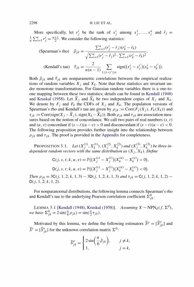
Both ρjk and τjk are nonparametric correlations between the empirical realiza-tions of random variables Xj and Xk . Note that these statistics are invariant un-der monotone transformations. For Gaussian random variables there is a one-to-one mapping between these two statistics; details can be found in Kendall (1948)and Kruskal (1958). Let Xj and Xk be two independent copies of Xj and Xk .We denote by Fj and Fk the CDFs of Xj and Xk . The population versions ofSpearman’s rho and Kendall’s tau are given by ρjk := Corr(Fj (Xj ),Fk(Xk)) andτjk := Corr(sign(Xj −Xj ), sign(Xk −Xk)). Both ρjk and τjk are association mea-sures based on the notion of concordance. We call two pairs of real numbers (s, t)

and (u, v) concordant if (s − t)(u−v) > 0 and disconcordant if (s − t)(u−v) < 0.The following proposition provides further insight into the relationship betweenρjk and τjk . The proof is provided in the Appendix for completeness.

PROPOSITION 3.1. Let (X(1)j ,X

(1)k ), (X

(2)j ,X

(2)k ) and (X

(3)j ,X

(3)k ) be three in-

dependent random vectors with the same distribution as (Xj ,Xk). Define

C(j, s, t;k,u, v) = P((

X(s)j − X

(t)j

)(X

(u)k − X

(v)k

)> 0

),

D(j, s, t;k,u, v) = P((

X(s)j − X

(t)j

)(X

(u)k − X

(v)k

)< 0

).

Then ρjk = 3C(j,1,2;k,1,3) − 3D(j,1,2;k,1,3) and τjk = C(j,1,2;k,1,2) −D(j,1,2;k,1,2).

For nonparanormal distributions, the following lemma connects Spearman’s rhoand Kendall’s tau to the underlying Pearson correlation coefficient �0

jk .

LEMMA 3.1 [Kendall (1948), Kruskal (1958)]. Assuming X ∼ NPNd(f,�0),we have �0

jk = 2 sin(π6 ρjk) = sin(π

2 τjk).

Motivated by this lemma, we define the following estimators Sρ = [Sρjk] and

Sτ = [Sτjk] for the unknown correlation matrix �0:

Sρjk =

⎧⎨⎩2 sin(

π

6ρjk

), j �= k,

1, j = k,


and

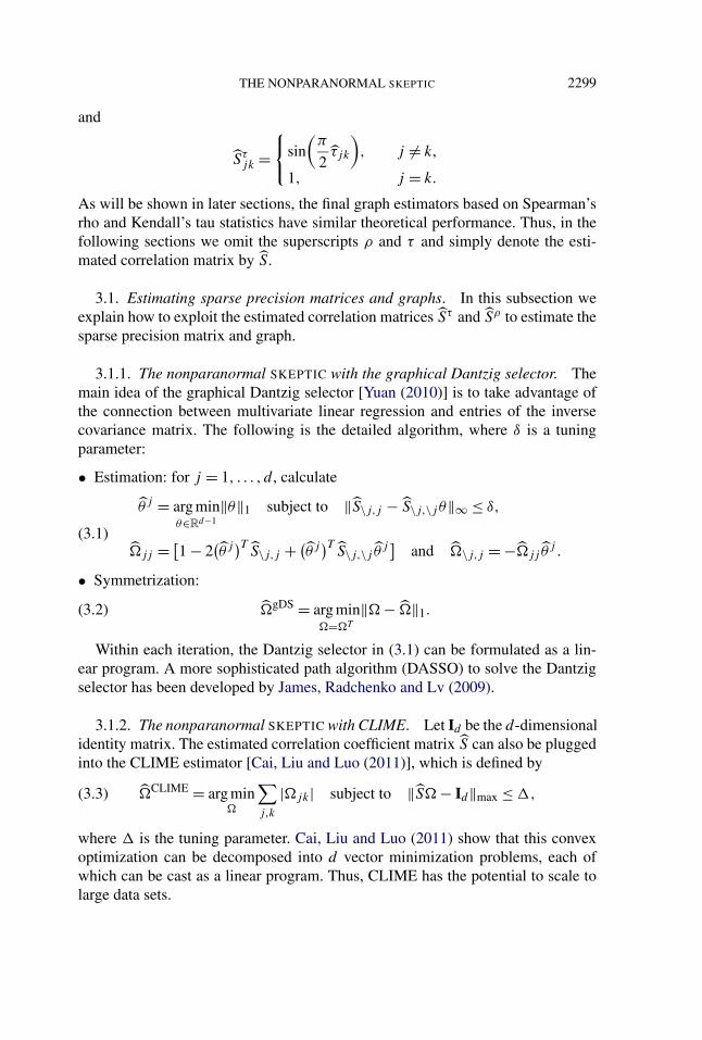
Sτjk =

⎧⎨⎩ sin(

π

2τjk

), j �= k,

1, j = k.

As will be shown in later sections, the final graph estimators based on Spearman’srho and Kendall’s tau statistics have similar theoretical performance. Thus, in thefollowing sections we omit the superscripts ρ and τ and simply denote the esti-mated correlation matrix by S.

3.1. Estimating sparse precision matrices and graphs. In this subsection weexplain how to exploit the estimated correlation matrices Sτ and Sρ to estimate thesparse precision matrix and graph.

3.1.1. The nonparanormal SKEPTIC with the graphical Dantzig selector. Themain idea of the graphical Dantzig selector [Yuan (2010)] is to take advantage ofthe connection between multivariate linear regression and entries of the inversecovariance matrix. The following is the detailed algorithm, where δ is a tuningparameter:

• Estimation: for j = 1, . . . , d , calculate

θ j = arg minθ∈Rd−1

‖θ‖1 subject to ‖S\j,j − S\j,\j θ‖∞ ≤ δ,

(3.1)�jj = [

1 − 2(θ j )T S\j,j + (

θ j )T S\j,\j θ j ] and �\j,j = −�jj θj .

• Symmetrization:

�gDS = arg min�=�T

‖� − �‖1.(3.2)

Within each iteration, the Dantzig selector in (3.1) can be formulated as a lin-ear program. A more sophisticated path algorithm (DASSO) to solve the Dantzigselector has been developed by James, Radchenko and Lv (2009).

3.1.2. The nonparanormal SKEPTIC with CLIME. Let Id be the d-dimensionalidentity matrix. The estimated correlation coefficient matrix S can also be pluggedinto the CLIME estimator [Cai, Liu and Luo (2011)], which is defined by

�CLIME = arg min�

∑j,k

|�jk| subject to ‖S� − Id‖max ≤ �,(3.3)

where � is the tuning parameter. Cai, Liu and Luo (2011) show that this convexoptimization can be decomposed into d vector minimization problems, each ofwhich can be cast as a linear program. Thus, CLIME has the potential to scale tolarge data sets.

2300 H. LIU ET AL.

3.1.3. The nonparanormal SKEPTIC with the graphical lasso. We can alsoplug the estimated correlation matrix S into the graphical lasso:

�glasso = arg min��0

{tr(S�) − log|�| + λ

∑j,k

|�jk|}.(3.4)

One thing to note is that S may not be positive semidefinite. Even though the for-mulation (3.4) is still convex, certain algorithms (like the blockwise-coordinatedescent algorithm [Friedman, Hastie and Tibshirani (2008)]) may fail if S is in-definite. However, other algorithms like the two-metric projected Newton methodor first-order projection do not have such positive semidefinite assumption on S.These algorithms can be directly exploited to efficiently solve (3.4).

Unlike the graphical Lasso formulation, the graphical Dantzig selector andCLIME can both be formulated as linear programs, so they do not require posi-tive semidefiniteness of the input correlation matrix.

3.1.4. The nonparanormal SKEPTIC with the neighborhood pursuit estimator(the Meinshausen–Bühlmann procedure). The nonparanormal SKEPTIC can alsobe applied with the Meinshausen–Bühlmann procedure to estimate the graph. Ashas been discussed in Friedman, Hastie and Tibshirani (2008), the correlation ma-trix is a sufficient statistic for the Meinshausen–Bühlmann procedure. However,in this case, we need to make sure that S is positive semidefinite. Otherwise, thealgorithm may not converge. Practically, we can first project S into the cone ofpositive semidefinite matrices. In particular, we need to solve the following con-vex optimization problem:

S = arg minS�0

‖S − S‖max.(3.5)

Here we use the ‖ · ‖max-norm instead of the ‖ · ‖F -norm, due to theoretical con-cerns developed in the next section. In fact, the optimization problem in (3.5) canbe formulated as the dual of a graphical lasso problem. To find the projection so-lution, we need to search for the smallest possible tuning parameter which stillmakes the optimization problem feasible. Empirically, we can use a surrogate pro-jection procedure that computes a singular value decomposition of S and truncatesall of the negative singular values to be zero.

3.2. Computational complexity. Compared to the corresponding parametricmethods like the graphical lasso, graphical Dantzig selector, CLIME and theMeinshausen–Bühlmann estimator, the only extra cost of the nonparanormalSKEPTIC is the computation of S, which requires us to calculate the d(d − 1)/2pairs of Spearman’s rho or Kendall’s tau statistics. A naive implementation ofKendall’s tau statistic requires O(n2) flops. However, an efficient algorithm basedon sorting and balanced binary trees has been developed to calculate Kendall’s taustatistic with complexity O(n logn). Details can be found in Christensen (2005).


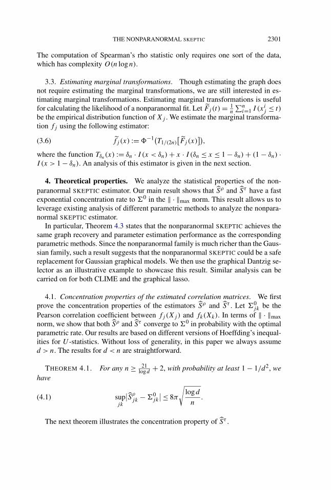
The computation of Spearman’s rho statistic only requires one sort of the data,which has complexity O(n logn).

3.3. Estimating marginal transformations. Though estimating the graph doesnot require estimating the marginal transformations, we are still interested in es-timating marginal transformations. Estimating marginal transformations is usefulfor calculating the likelihood of a nonparanormal fit. Let Fj (t) = 1

n

∑ni=1 I (xi

j ≤ t)

be the empirical distribution function of Xj . We estimate the marginal transforma-tion fj using the following estimator:

fj (x) := �−1(T1/(2n)

[Fj (x)

]),(3.6)

where the function Tδn(x) := δn · I (x < δn) + x · I (δn ≤ x ≤ 1 − δn) + (1 − δn) ·I (x > 1 − δn). An analysis of this estimator is given in the next section.

4. Theoretical properties. We analyze the statistical properties of the non-paranormal SKEPTIC estimator. Our main result shows that Sρ and Sτ have a fastexponential concentration rate to �0 in the ‖ · ‖max norm. This result allows us toleverage existing analysis of different parametric methods to analyze the nonpara-normal SKEPTIC estimator.

In particular, Theorem 4.3 states that the nonparanormal SKEPTIC achieves thesame graph recovery and parameter estimation performance as the correspondingparametric methods. Since the nonparanormal family is much richer than the Gaus-sian family, such a result suggests that the nonparanormal SKEPTIC could be a safereplacement for Gaussian graphical models. We then use the graphical Dantzig se-lector as an illustrative example to showcase this result. Similar analysis can becarried on for both CLIME and the graphical lasso.

4.1. Concentration properties of the estimated correlation matrices. We firstprove the concentration properties of the estimators Sρ and Sτ . Let �0

jk be thePearson correlation coefficient between fj (Xj ) and fk(Xk). In terms of ‖ · ‖maxnorm, we show that both Sρ and Sτ converge to �0 in probability with the optimalparametric rate. Our results are based on different versions of Hoeffding’s inequal-ities for U -statistics. Without loss of generality, in this paper we always assumed > n. The results for d < n are straightforward.

THEOREM 4.1. For any n ≥ 21logd

+ 2, with probability at least 1 − 1/d2, wehave

supjk

∣∣Sρjk − �0

jk

∣∣≤ 8π

√logd

n.(4.1)

The next theorem illustrates the concentration property of Sτ .

2302 H. LIU ET AL.

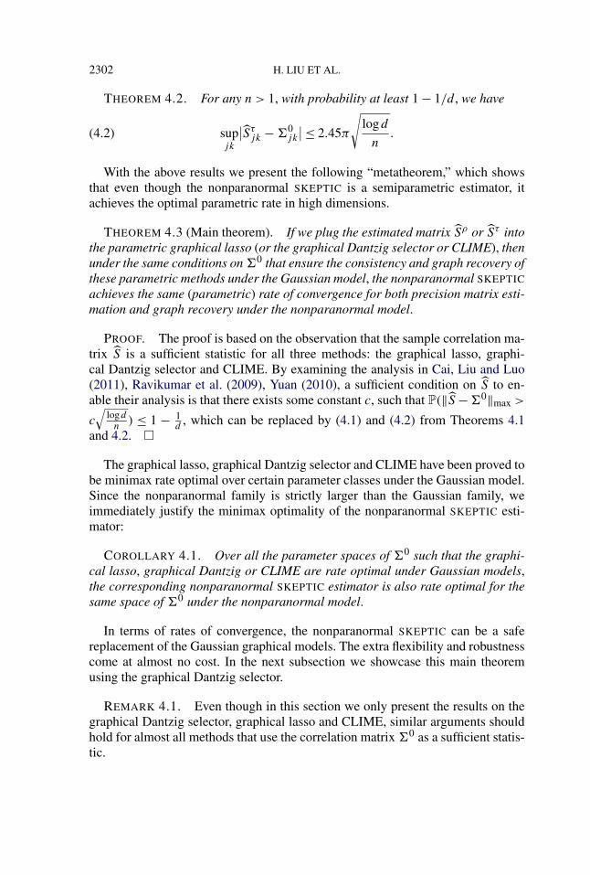
THEOREM 4.2. For any n > 1, with probability at least 1 − 1/d , we have

supjk

∣∣Sτjk − �0

jk

∣∣≤ 2.45π

√logd

n.(4.2)

With the above results we present the following “metatheorem,” which showsthat even though the nonparanormal SKEPTIC is a semiparametric estimator, itachieves the optimal parametric rate in high dimensions.

THEOREM 4.3 (Main theorem). If we plug the estimated matrix Sρ or Sτ intothe parametric graphical lasso (or the graphical Dantzig selector or CLIME), thenunder the same conditions on �0 that ensure the consistency and graph recovery ofthese parametric methods under the Gaussian model, the nonparanormal SKEPTIC

achieves the same (parametric) rate of convergence for both precision matrix esti-mation and graph recovery under the nonparanormal model.

PROOF. The proof is based on the observation that the sample correlation ma-trix S is a sufficient statistic for all three methods: the graphical lasso, graphi-cal Dantzig selector and CLIME. By examining the analysis in Cai, Liu and Luo(2011), Ravikumar et al. (2009), Yuan (2010), a sufficient condition on S to en-able their analysis is that there exists some constant c, such that P(‖S −�0‖max >

c

√logd

n) ≤ 1 − 1

d, which can be replaced by (4.1) and (4.2) from Theorems 4.1

and 4.2. �

The graphical lasso, graphical Dantzig selector and CLIME have been proved tobe minimax rate optimal over certain parameter classes under the Gaussian model.Since the nonparanormal family is strictly larger than the Gaussian family, weimmediately justify the minimax optimality of the nonparanormal SKEPTIC esti-mator:

COROLLARY 4.1. Over all the parameter spaces of �0 such that the graphi-cal lasso, graphical Dantzig or CLIME are rate optimal under Gaussian models,the corresponding nonparanormal SKEPTIC estimator is also rate optimal for thesame space of �0 under the nonparanormal model.

In terms of rates of convergence, the nonparanormal SKEPTIC can be a safereplacement of the Gaussian graphical models. The extra flexibility and robustnesscome at almost no cost. In the next subsection we showcase this main theoremusing the graphical Dantzig selector.

REMARK 4.1. Even though in this section we only present the results on thegraphical Dantzig selector, graphical lasso and CLIME, similar arguments shouldhold for almost all methods that use the correlation matrix �0 as a sufficient statis-tic.


4.2. Applying the nonparanormal SKEPTIC with the graphical Dantzig selector.In Theorem 4.3 we have shown that the nonparanormal SKEPTIC estimator S canbe plugged into any parametric procedure and can achieve the optimal parametricrate of convergence. In this subsection we use the graphical Dantzig selector as anexample to see how this theorem can be applied in specific applications.

We denote �npn-s to be the inverse correlation matrix estimated using the non-paranormal SKEPTIC with the graphical Dantzig selector in (3.2). Given a ma-trix �, we define deg(�) = max1≤i≤d

∑dj=1 I (|�ij | �= 0). Following Yuan (2010),

we consider a class of inverse correlation matrices: M1(κ, τ,M) := {� :� � 0,diag(�−1) = 1,‖�‖1 ≤ κ, 1

τ≤ λmin(�) ≤ λmax(�) ≤ τ,deg(�) ≤ M}, where

κ, τ > 1. We then have the following corollary of Theorem 4.3.

THEOREM 4.4. For 1 ≤ q ≤ ∞, there exists a constant C1 that depends on κ ,τ , λmin(�

0) and λmax(�0), such that

sup�0∈M1(κ,τ,M)

∥∥�npn-s − �0∥∥q = OP

(M

√logd

n

),

provided that limn→∞ nM2 logd

= ∞ and δ = C1

√logd

n, for sufficiently large C1.

Here δ is the tuning parameter used in (3.1).

PROOF. The proof can be directly obtained by replacing Lemma 12 in Yuan(2010) with the result of Theorem 4.3. �

The next theorem establishes the minimax lower bound for inverse correlationmatrix estimation over the class M1(κ, τ,M). Its proof can be easily obtained bya modification of Theorem 5 in Yuan (2010).

THEOREM 4.5 [Yuan (2010)]. Let M(logd/n)1/2 = o(1). Then there exists aconstant C > 0 depending only on κ and τ such that

lim infn→∞ inf

�sup

�0∈M1(κ,τ,M)

P

(∥∥� − �0∥∥1 ≥ CM

√logd

n

)> 0,

where the infimum is taken over all estimates of � based on the observed datax1, . . . , xn.

From the above theorems, we see that the nonparanormal SKEPTIC estimatorof the inverse correlation matrix can achieve the parametric rate and is in factminimax rate optimal over the parameter space M1(κ, τ,M) in terms of �1-risk.

2304 H. LIU ET AL.

4.3. Estimating marginal transformations. Recall the definition of fj (t) in(3.6). For any fixed t , fj (t) converges in probability to fj (t). Theorem 4.6 pro-vides a stronger result that fj converges to fj uniformly over an expanding inter-val. This result is important for many downstream applications of nonparanormalmodeling, for example, discriminant analysis or principle component analysis; de-tails will be provided in a follow-up paper.

THEOREM 4.6. Let gj := f −1j be the inverse function of fj . For any

0 < γ < 1, define In := [gj (−√

74(1 − γ ) logn), gj (

√74(1 − γ ) logn)]. Then

supt∈In|fj (t) − fj (t)| = oP (1).

5. Experimental results. We investigate the empirical performance of differ-ent graph estimation methods on both synthetic and real data sets. In particular,we consider the following methods: (i) npn—the original nonparanormal estima-tor from Liu, Lafferty and Wasserman (2009); (ii) normal—the Gaussian graph-ical model (which relies on the Gaussian assumption); (iii) npn-spearman—thenonparanormal SKEPTIC using Spearman’s rho; (iv) npn-tau—the nonparanormalSKEPTIC using Kendall’s tau; (v) npn-ns—the normal-score based estimator de-fined in (2.1) with δn = 1

n+1 .

5.1. Summary of the results. To compare the graph estimation performance oftwo procedures A and B , in the following we use A >slightly B to represent that A

slightly outperforms B; A > B means that A is better than B; A � B means thatA is significantly better than B; while A ≈ B means that A and B have similarperformance. Here we summarize the main results:

• Non-Gaussian data without outliers: npn-ns ≈ npn ≈ npn-spearman ≈ npn-tau � normal.

• Non-Gaussian data with a low level of outliers: npn-tau ≈ npn-spearman >

npn > npn-ns � normal.• Non-Gaussian data with a higher level of outliers: npn-tau > npn-spearman �

npn > npn-ns � normal.• Gaussian data without outliers: normal ≈ npn-ns ≈ npn >slightly npn-

spearman ≈ npn-tau.• Gaussian data with a low level of outliers: npn-tau ≈ npn-spearman > npn >

npn-ns � normal.• Gaussian data with a higher level of outliers: npn-tau > npn-spearman > npn >

npn-ns > normal.

These results indicate a trade-off between estimation robustness and statisti-cal efficiency. For nonparanormal data without outliers, npn-ns and npn behavesimilarly to npn-tau and npn-spearman. However, if the data are contaminated byoutliers, npn-tau and npn-spearman outperform npn-ns and npn even when the


contamination level is low. Overall, our simulations suggest that both npn-tau andnpn-spearman have a good balance of statistical efficiency and robustness. In addi-tion, since both the nonparanormal SKEPTIC and the normal-score based methodsare rank-based, they are invariant to different choices of marginal transformationsfj in the true model. In contrast, the Gaussian estimators (the graphical Lasso,CLIME, etc.) are not marginal transformation invariant. Their performance de-creases dramatically when nonidentity transformations are applied. Going beyondnumerical simulations, we also apply our method to a large-scale genomic data set.

5.2. Numerical simulations. We adopt the same data generating procedure asin Liu, Lafferty and Wasserman (2009). To generate a d-dimensional sparse graphG = (V ,E), let V = {1, . . . , d} correspond to variables X = (X1, . . . ,Xd). We as-sociate each index j ∈ {1, . . . , d} with a bivariate data point (Y

(1)j , Y

(2)j ) ∈ [0,1]2,

where Y(k)1 , . . . , Y

(k)d ∼ Uniform[0,1] for k = 1,2. Each pair of vertices (i, j) is

included in the edge set E with probability P((i, j) ∈ E) = 1√2π

exp(−‖yi−yj‖2

2s),

where yi := (y(1)i , y

(2)i ) is the empirical observation of (Y

(1)i , Y

(2)i ) and ‖ · ‖ de-

notes Euclidean distance. Here, s = 0.125 is a parameter that controls the spar-sity level of the generated graph. We restrict the maximum degree of the graphto be 4 and build the inverse correlation matrix �0 according to �0

jk = 1 if j = k,

�0jk = 0.245 if (j, k) ∈ E, and �0

jk = 0 otherwise. Here the value 0.245 guarantees

positive definiteness of �0. Let �0 = (�0)−1. To obtain the correlation matrix, wesimply rescale �0 so that all its diagonal elements are 1. We then sample n datapoints x1, . . . , xn from the nonparanormal distribution NPNd(f 0,�0), where forsimplicity we use the same univariate transformations on each dimension, that is,f 0

1 = · · · = f 0d = f 0. To sample data from the nonparanormal distribution, we also

need g0 := (f 0)−1. The following two different versions of g0 are used in thesimulations:

DEFINITION 5.1 (Gaussian CDF transformation). Let g0 be a univariateGaussian cumulative distribution function with mean μg0 and the standard devia-

tion σg0 :g0(t) := �(t−μg0σg0

). The Gaussian CDF transformation g0j = (f 0

j )−1 for

the j th dimension is defined as

g0j (zj ) := g0(zj ) − ∫

g0(t)φ((t − μj)/σj ) dt√∫(g0(y) − ∫

g0(t)φ((t − μj)/σj ) dt)2φ((y − μj)/σj ) dy,(5.1)

where φ(·) is the standard Gaussian density function.

DEFINITION 5.2 (Power transformation). Let g0(t) := sign(t)|t |α whereα > 0 is a parameter. The power transformation for the j th dimension is defined

2306 H. LIU ET AL.

as

g0j (zj ) := g0(zj − μj)√∫

g20(t − μj)φ((t − μj)/σj ) dt

,(5.2)

where φ(·) is the standard Gaussian density function.

These transformations were used by Liu, Lafferty and Wasserman (2009) tostudy the performance of the original nonparanormal estimator. To comply withtheir simulation design, for the Gaussian CDF transformation we set μg0 = 0.05and σg0 = 0.4; for the power transformation, we set α = 3.

To generate synthetic data, we set d = 100, resulting in(100

2

)+ 100 = 5050 pa-rameters to be estimated. The sample sizes vary from n = 100,200 to 500. Threeconditions are considered, corresponding to using the power transformation, theGaussian CDF transformation and the linear transformation (or no transforma-tion).3

To evaluate the robustness of these methods, we consider two types of data con-tamination mechanisms, deterministic contamination and random contamination.Let r ∈ (0,1) be the contamination level. For deterministic contamination we re-place �nr� data points with a deterministic vector (+5,−5,+5,−5,+5, . . .)T ∈R

d , in which the numbers +5 and −5 occur in an alternating way. For random con-tamination, we randomly (according to a uniform distribution) select �nr� entriesof each dimension and replace them with either +5 or −5 with equal probabil-ity. From the robustness point of view, the deterministic contamination is moremalicious and can severely hurt nonrobust procedures. In contrast, the randomcontamination is relatively benign and is more realistic for modern scientific dataanalysis.

Both the normal-score based nonparanormal estimators (npn and npn-ns) andthe nonparanormal SKEPTIC estimators (npn-spearman and npn-tau) are two-stepprocedures. In the first step we obtain an estimate S of the correlation matrix; inthe second step we plug S into a parametric graph estimation procedure. In thisnumerical study, we consider two parametric baseline procedures: (i) the graphi-cal lasso and (ii) the Meinshausen–Bühlmann graph estimator. The former repre-sents the likelihood-based approach and the latter is a type of pseudo-likelihood-based approach. In our experiments, we find that CLIME has behavior similarto the graphical lasso, while the graphical Dantzig selector behaves similarly tothe Meinshausen–Bühlmann method. Our implementations of the nonparanormalSKEPTIC, graphical lasso and Meinshausen–Bühlmann methods are available inthe R package huge.4

3For linear transformation, the data exactly follow the Gaussian distribution.4http://cran.r-project.org/web/packages/huge. The package huge corrects some nonconvergence

problems in the glasso package.

http://cran.r-project.org/web/packages/huge


Let G = (V ,E) be a d-dimensional graph. We denote by |E| the number ofedges in the graph G. We use false positive and negative rates to evaluate thegraph estimation performance. Let Gλ = (V , Eλ) be an estimated graph usingthe regularization parameter λ in either the graphical lasso procedure (3.4) or theMeinshausen–Bühlmann procedure. The number of false positives when using theregularization parameter λ is FP(λ) := the number of edges in Eλ but not in E.The number of false negatives at λ is defined as FN(λ) := the number of edges inE but not in Eλ. We further define the false negative rate (FNR) and false positiverate (FPR) as

FNR(λ) := FN(λ)

|E| and FPR(λ) := FP(λ)/[(d

2

)− |E|

].(5.3)

Let � be the set of all regularization parameters used to create the full path. Theoracle regularization parameter λ∗ is defined as

λ∗ := arg minλ∈�

{FNR(λ) + FPR(λ)

}.

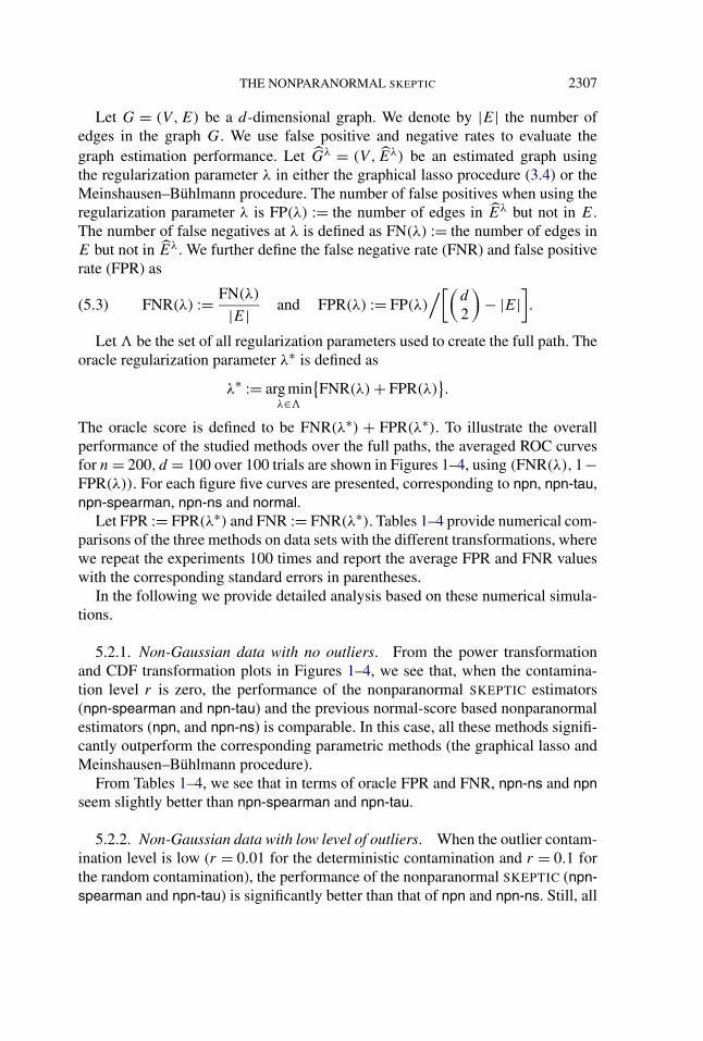
The oracle score is defined to be FNR(λ∗) + FPR(λ∗). To illustrate the overallperformance of the studied methods over the full paths, the averaged ROC curvesfor n = 200, d = 100 over 100 trials are shown in Figures 1–4, using (FNR(λ),1−FPR(λ)). For each figure five curves are presented, corresponding to npn, npn-tau,npn-spearman, npn-ns and normal.

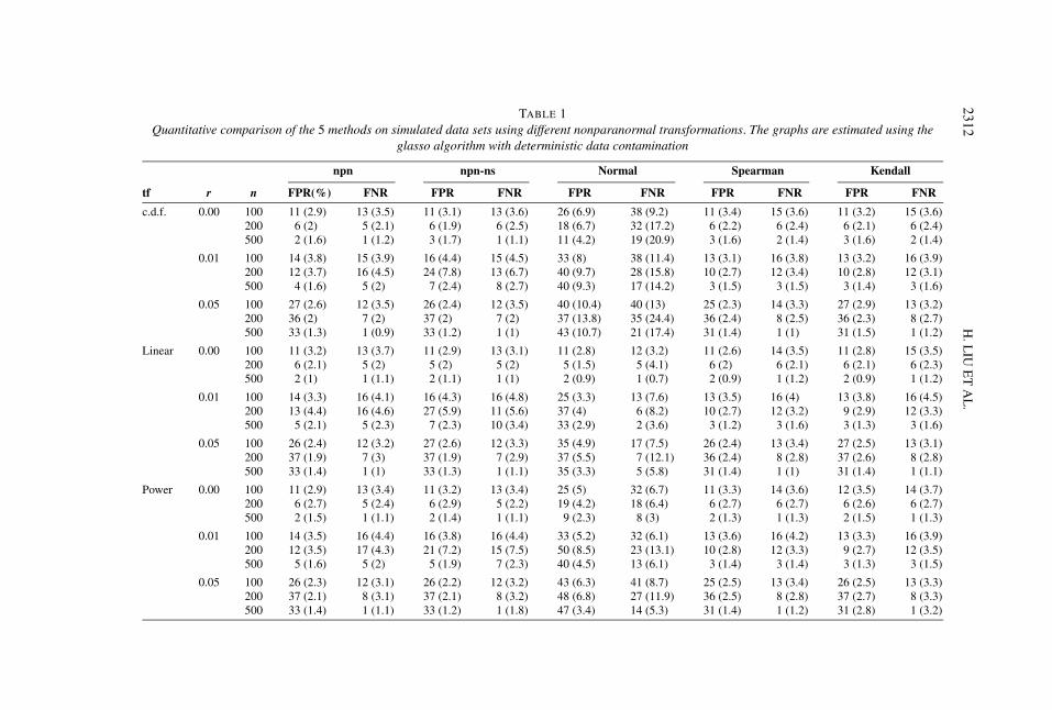
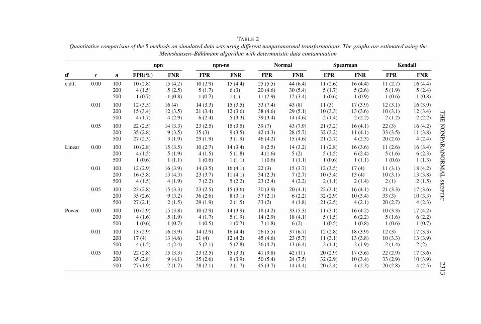
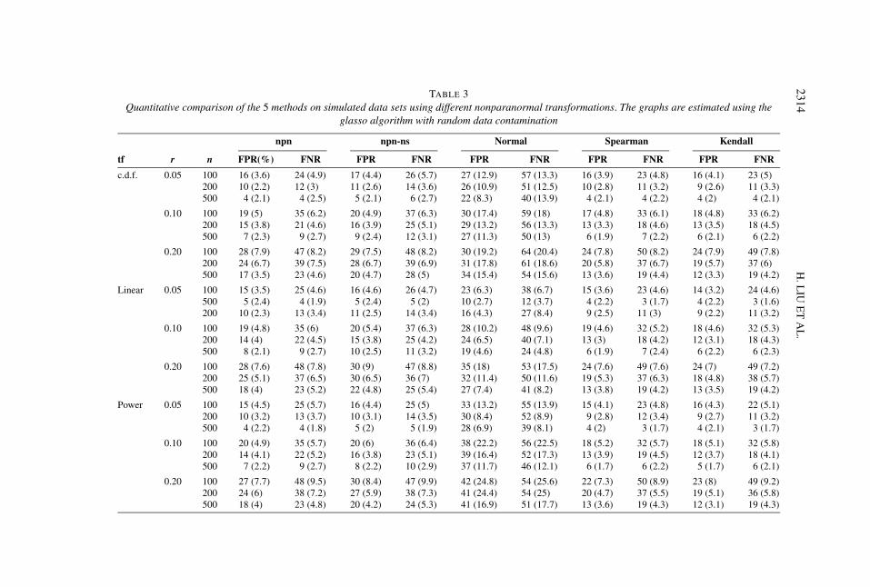
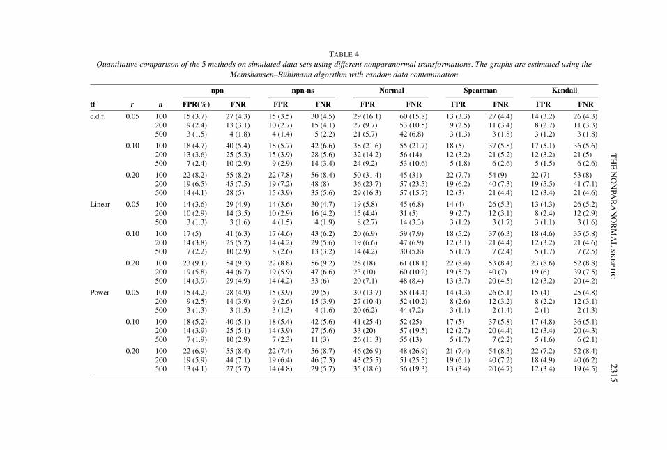
Let FPR := FPR(λ∗) and FNR := FNR(λ∗). Tables 1–4 provide numerical com-parisons of the three methods on data sets with the different transformations, wherewe repeat the experiments 100 times and report the average FPR and FNR valueswith the corresponding standard errors in parentheses.

In the following we provide detailed analysis based on these numerical simula-tions.

5.2.1. Non-Gaussian data with no outliers. From the power transformationand CDF transformation plots in Figures 1–4, we see that, when the contamina-tion level r is zero, the performance of the nonparanormal SKEPTIC estimators(npn-spearman and npn-tau) and the previous normal-score based nonparanormalestimators (npn, and npn-ns) is comparable. In this case, all these methods signifi-cantly outperform the corresponding parametric methods (the graphical lasso andMeinshausen–Bühlmann procedure).

From Tables 1–4, we see that in terms of oracle FPR and FNR, npn-ns and npnseem slightly better than npn-spearman and npn-tau.

5.2.2. Non-Gaussian data with low level of outliers. When the outlier contam-ination level is low (r = 0.01 for the deterministic contamination and r = 0.1 forthe random contamination), the performance of the nonparanormal SKEPTIC (npn-spearman and npn-tau) is significantly better than that of npn and npn-ns. Still, all

2308 H. LIU ET AL.

FIG. 1. ROC curves for the c.d.f., linear and power transformations (top, middle, bottom) using theMeinshausen–Bühlmann graph estimator, with deterministic data contamination at different levels(r = 0, 0.01, 0.05). Here n = 200 and d = 100. Note: “npn” is the original Winsorized normal-s-core nonparanormal estimator from Liu, Lafferty and Wasserman (2009); “normal” is the naiveGaussian graph estimator; “Spearman” represents the nonparanormal SKEPTIC using Spearman’srho; “Kendall” represents the nonparanormal SKEPTIC using Kendall’s tau; “npn-ns” representsthe normal-score based nonparanormal estimator.

the semiparametric methods significantly outperform the corresponding paramet-ric methods (the graphical lasso and parallel lasso procedure). Similar patterns canalso be found based on the quantitative comparisons in Tables 1–4.

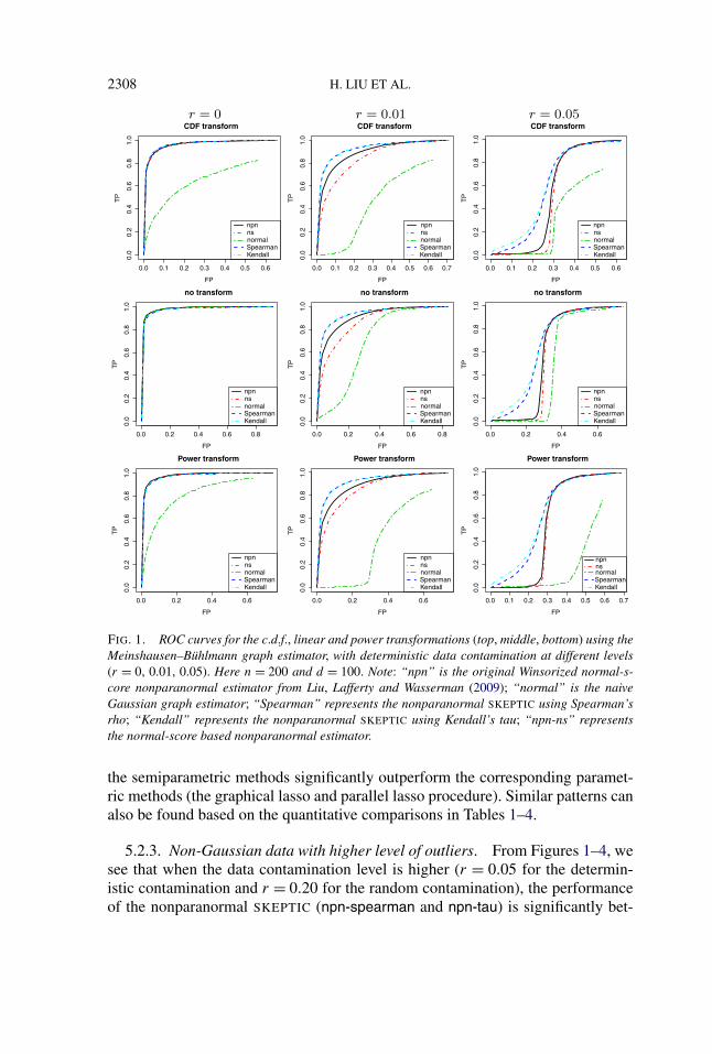
5.2.3. Non-Gaussian data with higher level of outliers. From Figures 1–4, wesee that when the data contamination level is higher (r = 0.05 for the determin-istic contamination and r = 0.20 for the random contamination), the performanceof the nonparanormal SKEPTIC (npn-spearman and npn-tau) is significantly bet-


FIG. 2. ROC curves for the c.d.f., linear and power transformations (top, middle, bottom) using theglasso graph estimator, with deterministic data contamination at different levels (r = 0, 0.01, 0.05),with n = 200 and d = 100.

ter than that of npn and npn-ns. For this high outlier case, npn-tau outperformsnpn-spearman, suggesting that Kendall’s tau is more robust than Spearman’s rhostatistic. The parametric methods (the graphical lasso and parallel lasso procedure)perform the worst.

Unlike the previous low outlier case, the quantitative results from Tables 1–4present interesting patterns. For deterministic contamination, we do not see signif-icant improvement of the npn-spearman and npn-tau over npn and npn-ns in termsof the oracle FPR and FNR. At first sight this seems counterintuitive since the cor-responding ROC curves suggest that npn-spearman and npn-tau are globally bet-ter than npn and npn-ns. The main reason for such a result is that the oracle scorepoint happens to coincide with the intersection point of different ROC curves. On

2310 H. LIU ET AL.

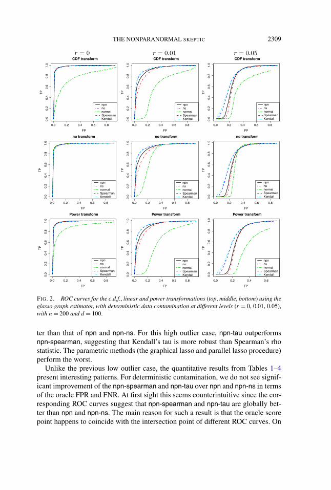
FIG. 3. ROC curves for the c.d.f., linear and power transformations (top, middle, bottom) using theglasso graph estimator, with random data contamination at different levels (r = 0.05, 0.1, 0.2), withn = 200 and d = 100.

the other hand, for the random contamination setting, we see that the performanceof npn-spearman and npn-tau uniformly dominates that of the npn and npn-ns.

5.2.4. Gaussian data with no outliers. From the linear transformation plot inFigures 1–4, we see that when the outlier contamination level is r = 0 the perfor-mance of all these methods is comparable. Based on Tables 1–4, we could see thatin terms of oracle FPR and FNR, normal, npn-ns and npn are slightly better thannpn-spearman and npn-tau. This result suggests that there is only a very small ef-ficiency loss for the nonparanormal SKEPTIC with truly Gaussian data, though thisloss seems negligible.


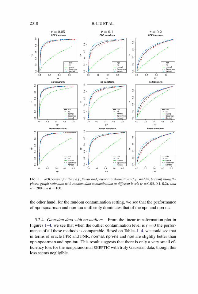
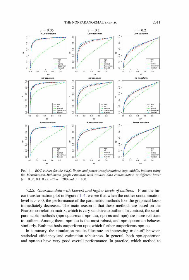
FIG. 4. ROC curves for the c.d.f., linear and power transformations (top, middle, bottom) usingthe Meinshausen–Bühlmann graph estimator, with random data contamination at different levels(r = 0.05, 0.1, 0.2), with n = 200 and d = 100.

5.2.5. Gaussian data with Lowerk and higher levels of outliers. From the lin-ear transformation plot in Figures 1–4, we see that when the outlier contaminationlevel is r > 0, the performance of the parametric methods like the graphical lassoimmediately decreases. The main reason is that these methods are based on thePearson correlation matrix, which is very sensitive to outliers. In contrast, the semi-parametric methods (npn-spearman, npn-tau, npn-ns and npn) are more resistantto outliers. Among them, npn-tau is the most robust, and npn-spearman behavessimilarly. Both methods outperform npn, which further outperforms npn-ns.

In summary, the simulation results illustrate an interesting trade-off betweenstatistical efficiency and estimation robustness. In general, both npn-spearmanand npn-tau have very good overall performance. In practice, which method to

2312H

.LIU

ET

AL

.

TABLE 1Quantitative comparison of the 5 methods on simulated data sets using different nonparanormal transformations. The graphs are estimated using the

glasso algorithm with deterministic data contamination

npn npn-ns Normal Spearman Kendall

tf r n FPR(%) FNR FPR FNR FPR FNR FPR FNR FPR FNR

c.d.f. 0.00 100 11 (2.9) 13 (3.5) 11 (3.1) 13 (3.6) 26 (6.9) 38 (9.2) 11 (3.4) 15 (3.6) 11 (3.2) 15 (3.6)200 6 (2) 5 (2.1) 6 (1.9) 6 (2.5) 18 (6.7) 32 (17.2) 6 (2.2) 6 (2.4) 6 (2.1) 6 (2.4)500 2 (1.6) 1 (1.2) 3 (1.7) 1 (1.1) 11 (4.2) 19 (20.9) 3 (1.6) 2 (1.4) 3 (1.6) 2 (1.4)

0.01 100 14 (3.8) 15 (3.9) 16 (4.4) 15 (4.5) 33 (8) 38 (11.4) 13 (3.1) 16 (3.8) 13 (3.2) 16 (3.9)200 12 (3.7) 16 (4.5) 24 (7.8) 13 (6.7) 40 (9.7) 28 (15.8) 10 (2.7) 12 (3.4) 10 (2.8) 12 (3.1)500 4 (1.6) 5 (2) 7 (2.4) 8 (2.7) 40 (9.3) 17 (14.2) 3 (1.5) 3 (1.5) 3 (1.4) 3 (1.6)

0.05 100 27 (2.6) 12 (3.5) 26 (2.4) 12 (3.5) 40 (10.4) 40 (13) 25 (2.3) 14 (3.3) 27 (2.9) 13 (3.2)200 36 (2) 7 (2) 37 (2) 7 (2) 37 (13.8) 35 (24.4) 36 (2.4) 8 (2.5) 36 (2.3) 8 (2.7)500 33 (1.3) 1 (0.9) 33 (1.2) 1 (1) 43 (10.7) 21 (17.4) 31 (1.4) 1 (1) 31 (1.5) 1 (1.2)

Linear 0.00 100 11 (3.2) 13 (3.7) 11 (2.9) 13 (3.1) 11 (2.8) 12 (3.2) 11 (2.6) 14 (3.5) 11 (2.8) 15 (3.5)200 6 (2.1) 5 (2) 5 (2) 5 (2) 5 (1.5) 5 (4.1) 6 (2) 6 (2.1) 6 (2.1) 6 (2.3)500 2 (1) 1 (1.1) 2 (1.1) 1 (1) 2 (0.9) 1 (0.7) 2 (0.9) 1 (1.2) 2 (0.9) 1 (1.2)

0.01 100 14 (3.3) 16 (4.1) 16 (4.3) 16 (4.8) 25 (3.3) 13 (7.6) 13 (3.5) 16 (4) 13 (3.8) 16 (4.5)200 13 (4.4) 16 (4.6) 27 (5.9) 11 (5.6) 37 (4) 6 (8.2) 10 (2.7) 12 (3.2) 9 (2.9) 12 (3.3)500 5 (2.1) 5 (2.3) 7 (2.3) 10 (3.4) 33 (2.9) 2 (3.6) 3 (1.2) 3 (1.6) 3 (1.3) 3 (1.6)

0.05 100 26 (2.4) 12 (3.2) 27 (2.6) 12 (3.3) 35 (4.9) 17 (7.5) 26 (2.4) 13 (3.4) 27 (2.5) 13 (3.1)200 37 (1.9) 7 (3) 37 (1.9) 7 (2.9) 37 (5.5) 7 (12.1) 36 (2.4) 8 (2.8) 37 (2.6) 8 (2.8)500 33 (1.4) 1 (1) 33 (1.3) 1 (1.1) 35 (3.3) 5 (5.8) 31 (1.4) 1 (1) 31 (1.4) 1 (1.1)

Power 0.00 100 11 (2.9) 13 (3.4) 11 (3.2) 13 (3.4) 25 (5) 32 (6.7) 11 (3.3) 14 (3.6) 12 (3.5) 14 (3.7)200 6 (2.7) 5 (2.4) 6 (2.9) 5 (2.2) 19 (4.2) 18 (6.4) 6 (2.7) 6 (2.7) 6 (2.6) 6 (2.7)500 2 (1.5) 1 (1.1) 2 (1.4) 1 (1.1) 9 (2.3) 8 (3) 2 (1.3) 1 (1.3) 2 (1.5) 1 (1.3)

0.01 100 14 (3.5) 16 (4.4) 16 (3.8) 16 (4.4) 33 (5.2) 32 (6.1) 13 (3.6) 16 (4.2) 13 (3.3) 16 (3.9)200 12 (3.5) 17 (4.3) 21 (7.2) 15 (7.5) 50 (8.5) 23 (13.1) 10 (2.8) 12 (3.3) 9 (2.7) 12 (3.5)500 5 (1.6) 5 (2) 5 (1.9) 7 (2.3) 40 (4.5) 13 (6.1) 3 (1.4) 3 (1.4) 3 (1.3) 3 (1.5)

0.05 100 26 (2.3) 12 (3.1) 26 (2.2) 12 (3.2) 43 (6.3) 41 (8.7) 25 (2.5) 13 (3.4) 26 (2.5) 13 (3.3)200 37 (2.1) 8 (3.1) 37 (2.1) 8 (3.2) 48 (6.8) 27 (11.9) 36 (2.5) 8 (2.8) 37 (2.7) 8 (3.3)500 33 (1.4) 1 (1.1) 33 (1.2) 1 (1.8) 47 (3.4) 14 (5.3) 31 (1.4) 1 (1.2) 31 (2.8) 1 (3.2)

TH

EN

ON

PAR

AN

OR

MA

LS

KE

PT

IC2313


Meinshausen–Bühlmann algorithm with deterministic data contamination



c.d.f. 0.00 100 10 (2.8) 15 (4.2) 10 (2.9) 15 (4.4) 25 (5.5) 44 (6.4) 11 (2.6) 16 (4.4) 11 (2.7) 16 (4.4)200 4 (1.5) 5 (2.5) 5 (1.7) 6 (3) 20 (4.6) 30 (5.4) 5 (1.7) 5 (2.6) 5 (1.9) 5 (2.4)500 1 (0.7) 1 (0.8) 1 (0.7) 1 (1) 11 (2.9) 12 (3.4) 1 (0.6) 1 (0.9) 1 (0.6) 1 (0.8)

0.01 100 12 (3.5) 16 (4) 14 (3.3) 15 (3.5) 33 (7.4) 43 (8) 11 (3) 17 (3.9) 12 (3.1) 16 (3.9)200 15 (3.4) 12 (3.5) 21 (3.4) 12 (3.6) 38 (4.6) 29 (5.1) 10 (3.3) 13 (3.6) 10 (3.1) 12 (3.4)500 4 (1.7) 4 (2.9) 6 (2.4) 5 (3.3) 39 (3.4) 14 (4.6) 2 (1.4) 2 (2.2) 2 (1.2) 2 (2.2)

0.05 100 22 (2.5) 14 (3.3) 23 (2.5) 15 (3.5) 39 (7) 43 (7.9) 21 (3.2) 16 (4.1) 22 (3) 16 (4.2)200 35 (2.8) 9 (3.5) 35 (3) 9 (3.5) 42 (4.3) 28 (5.7) 32 (3.2) 11 (4.1) 33 (3.5) 11 (3.8)500 27 (2.3) 3 (1.9) 29 (1.9) 3 (1.9) 46 (4.2) 15 (4.6) 21 (2.7) 4 (2.3) 20 (2.6) 4 (2.4)

Linear 0.00 100 10 (2.8) 15 (3.5) 10 (2.7) 14 (3.4) 9 (2.5) 14 (3.2) 11 (2.8) 16 (3.6) 11 (2.6) 16 (3.4)200 4 (1.5) 5 (1.9) 4 (1.5) 5 (1.8) 4 (1.6) 5 (2) 5 (1.5) 6 (2.4) 5 (1.6) 6 (2.3)500 1 (0.6) 1 (1.1) 1 (0.6) 1 (1.1) 1 (0.6) 1 (1.1) 1 (0.6) 1 (1.1) 1 (0.6) 1 (1.3)

0.01 100 12 (2.9) 16 (3.9) 14 (3.5) 16 (4.1) 22 (3) 15 (3.7) 12 (3.5) 17 (4) 11 (3.1) 18 (4.2)200 16 (3.8) 13 (4.3) 23 (3.7) 11 (4.1) 34 (2.3) 7 (2.7) 10 (3.4) 13 (4) 10 (3.1) 13 (3.8)500 4 (1.5) 4 (1.9) 7 (2.2) 5 (2.2) 23 (2.4) 4 (2.2) 2 (1.1) 2 (1.4) 2 (1) 2 (1.5)

0.05 100 23 (2.8) 15 (3.3) 23 (2.5) 15 (3.6) 30 (3.9) 20 (4.1) 22 (3.1) 16 (4.1) 21 (3.3) 17 (3.6)200 35 (2.6) 9 (3.2) 36 (2.6) 8 (3.1) 37 (2.1) 6 (2.2) 32 (2.9) 10 (3.4) 33 (3) 10 (3.3)500 27 (2.1) 2 (1.5) 29 (1.9) 2 (1.5) 33 (2) 4 (1.8) 21 (2.5) 4 (2.1) 20 (2.7) 4 (2.3)

Power 0.00 100 10 (2.9) 15 (3.8) 10 (2.9) 14 (3.9) 18 (4.2) 33 (5.3) 11 (3.1) 16 (4.2) 10 (3.3) 17 (4.2)200 4 (1.6) 5 (1.9) 4 (1.7) 5 (1.9) 14 (2.9) 18 (4.1) 5 (1.5) 6 (2.2) 5 (1.6) 6 (2.2)500 1 (0.6) 1 (0.7) 1 (0.5) 1 (0.7) 7 (1.8) 6 (2) 1 (0.5) 1 (0.8) 1 (0.6) 1 (0.7)

0.01 100 13 (2.9) 16 (3.9) 14 (2.9) 16 (4.4) 26 (5.5) 37 (6.7) 12 (2.8) 18 (3.9) 12 (3) 17 (3.3)200 17 (4) 13 (4.6) 21 (4) 12 (4.2) 45 (4.6) 23 (5.7) 11 (3.1) 13 (3.8) 10 (3.3) 13 (3.9)500 4 (1.5) 4 (2.4) 5 (2.1) 5 (2.8) 36 (4.2) 13 (6.4) 2 (1.1) 2 (1.9) 2 (1.4) 2 (2)

0.05 100 22 (2.8) 15 (3.3) 23 (2.5) 15 (3.3) 41 (9.8) 42 (11) 20 (2.9) 17 (3.6) 22 (2.9) 17 (3.6)200 35 (2.8) 9 (4.1) 35 (2.6) 9 (3.9) 50 (5.4) 24 (7.5) 32 (2.9) 10 (3.4) 33 (2.9) 10 (3.9)500 27 (1.9) 2 (1.7) 28 (2.1) 2 (1.7) 45 (3.7) 14 (4.4) 20 (2.4) 4 (2.3) 20 (2.8) 4 (2.5)

2314H

.LIU

ET

AL

.


glasso algorithm with random data contamination



c.d.f. 0.05 100 16 (3.6) 24 (4.9) 17 (4.4) 26 (5.7) 27 (12.9) 57 (13.3) 16 (3.9) 23 (4.8) 16 (4.1) 23 (5)200 10 (2.2) 12 (3) 11 (2.6) 14 (3.6) 26 (10.9) 51 (12.5) 10 (2.8) 11 (3.2) 9 (2.6) 11 (3.3)500 4 (2.1) 4 (2.5) 5 (2.1) 6 (2.7) 22 (8.3) 40 (13.9) 4 (2.1) 4 (2.2) 4 (2) 4 (2.1)

0.10 100 19 (5) 35 (6.2) 20 (4.9) 37 (6.3) 30 (17.4) 59 (18) 17 (4.8) 33 (6.1) 18 (4.8) 33 (6.2)200 15 (3.8) 21 (4.6) 16 (3.9) 25 (5.1) 29 (13.2) 56 (13.3) 13 (3.3) 18 (4.6) 13 (3.5) 18 (4.5)500 7 (2.3) 9 (2.7) 9 (2.4) 12 (3.1) 27 (11.3) 50 (13) 6 (1.9) 7 (2.2) 6 (2.1) 6 (2.2)

0.20 100 28 (7.9) 47 (8.2) 29 (7.5) 48 (8.2) 30 (19.2) 64 (20.4) 24 (7.8) 50 (8.2) 24 (7.9) 49 (7.8)200 24 (6.7) 39 (7.5) 28 (6.7) 39 (6.9) 31 (17.8) 61 (18.6) 20 (5.8) 37 (6.7) 19 (5.7) 37 (6)500 17 (3.5) 23 (4.6) 20 (4.7) 28 (5) 34 (15.4) 54 (15.6) 13 (3.6) 19 (4.4) 12 (3.3) 19 (4.2)

Linear 0.05 100 15 (3.5) 25 (4.6) 16 (4.6) 26 (4.7) 23 (6.3) 38 (6.7) 15 (3.6) 23 (4.6) 14 (3.2) 24 (4.6)500 5 (2.4) 4 (1.9) 5 (2.4) 5 (2) 10 (2.7) 12 (3.7) 4 (2.2) 3 (1.7) 4 (2.2) 3 (1.6)200 10 (2.3) 13 (3.4) 11 (2.5) 14 (3.4) 16 (4.3) 27 (8.4) 9 (2.5) 11 (3) 9 (2.2) 11 (3.2)

0.10 100 19 (4.8) 35 (6) 20 (5.4) 37 (6.3) 28 (10.2) 48 (9.6) 19 (4.6) 32 (5.2) 18 (4.6) 32 (5.3)200 14 (4) 22 (4.5) 15 (3.8) 25 (4.2) 24 (6.5) 40 (7.1) 13 (3) 18 (4.2) 12 (3.1) 18 (4.3)500 8 (2.1) 9 (2.7) 10 (2.5) 11 (3.2) 19 (4.6) 24 (4.8) 6 (1.9) 7 (2.4) 6 (2.2) 6 (2.3)

0.20 100 28 (7.6) 48 (7.8) 30 (9) 47 (8.8) 35 (18) 53 (17.5) 24 (7.6) 49 (7.6) 24 (7) 49 (7.2)200 25 (5.1) 37 (6.5) 30 (6.5) 36 (7) 32 (11.4) 50 (11.6) 19 (5.3) 37 (6.3) 18 (4.8) 38 (5.7)500 18 (4) 23 (5.2) 22 (4.8) 25 (5.4) 27 (7.4) 41 (8.2) 13 (3.8) 19 (4.2) 13 (3.5) 19 (4.2)

Power 0.05 100 15 (4.5) 25 (5.7) 16 (4.4) 25 (5) 33 (13.2) 55 (13.9) 15 (4.1) 23 (4.8) 16 (4.3) 22 (5.1)200 10 (3.2) 13 (3.7) 10 (3.1) 14 (3.5) 30 (8.4) 52 (8.9) 9 (2.8) 12 (3.4) 9 (2.7) 11 (3.2)500 4 (2.2) 4 (1.8) 5 (2) 5 (1.9) 28 (6.9) 39 (8.1) 4 (2) 3 (1.7) 4 (2.1) 3 (1.7)

0.10 100 20 (4.9) 35 (5.7) 20 (6) 36 (6.4) 38 (22.2) 56 (22.5) 18 (5.2) 32 (5.7) 18 (5.1) 32 (5.8)200 14 (4.1) 22 (5.2) 16 (3.8) 23 (5.1) 39 (16.4) 52 (17.3) 13 (3.9) 19 (4.5) 12 (3.7) 18 (4.1)500 7 (2.2) 9 (2.7) 8 (2.2) 10 (2.9) 37 (11.7) 46 (12.1) 6 (1.7) 6 (2.2) 5 (1.7) 6 (2.1)

0.20 100 27 (7.7) 48 (9.5) 30 (8.4) 47 (9.9) 42 (24.8) 54 (25.6) 22 (7.3) 50 (8.9) 23 (8) 49 (9.2)200 24 (6) 38 (7.2) 27 (5.9) 38 (7.3) 41 (24.4) 54 (25) 20 (4.7) 37 (5.5) 19 (5.1) 36 (5.8)500 18 (4) 23 (4.8) 20 (4.2) 24 (5.3) 41 (16.9) 51 (17.7) 13 (3.6) 19 (4.3) 12 (3.1) 19 (4.3)

TH

EN

ON

PAR

AN

OR

MA

LS

KE

PT

IC2315


Meinshausen–Bühlmann algorithm with random data contamination



c.d.f. 0.05 100 15 (3.7) 27 (4.3) 15 (3.5) 30 (4.5) 29 (16.1) 60 (15.8) 13 (3.3) 27 (4.4) 14 (3.2) 26 (4.3)200 9 (2.4) 13 (3.1) 10 (2.7) 15 (4.1) 27 (9.7) 53 (10.5) 9 (2.5) 11 (3.4) 8 (2.7) 11 (3.3)500 3 (1.5) 4 (1.8) 4 (1.4) 5 (2.2) 21 (5.7) 42 (6.8) 3 (1.3) 3 (1.8) 3 (1.2) 3 (1.8)

0.10 100 18 (4.7) 40 (5.4) 18 (5.7) 42 (6.6) 38 (21.6) 55 (21.7) 18 (5) 37 (5.8) 17 (5.1) 36 (5.6)200 13 (3.6) 25 (5.3) 15 (3.9) 28 (5.6) 32 (14.2) 56 (14) 12 (3.2) 21 (5.2) 12 (3.2) 21 (5)500 7 (2.4) 10 (2.9) 9 (2.9) 14 (3.4) 24 (9.2) 53 (10.6) 5 (1.8) 6 (2.6) 5 (1.5) 6 (2.6)

0.20 100 22 (8.2) 55 (8.2) 22 (7.8) 56 (8.4) 50 (31.4) 45 (31) 22 (7.7) 54 (9) 22 (7) 53 (8)200 19 (6.5) 45 (7.5) 19 (7.2) 48 (8) 36 (23.7) 57 (23.5) 19 (6.2) 40 (7.3) 19 (5.5) 41 (7.1)500 14 (4.1) 28 (5) 15 (3.9) 35 (5.6) 29 (16.3) 57 (15.7) 12 (3) 21 (4.4) 12 (3.4) 21 (4.6)

Linear 0.05 100 14 (3.6) 29 (4.9) 14 (3.6) 30 (4.7) 19 (5.8) 45 (6.8) 14 (4) 26 (5.3) 13 (4.3) 26 (5.2)200 10 (2.9) 14 (3.5) 10 (2.9) 16 (4.2) 15 (4.4) 31 (5) 9 (2.7) 12 (3.1) 8 (2.4) 12 (2.9)500 3 (1.3) 3 (1.6) 4 (1.5) 4 (1.9) 8 (2.7) 14 (3.3) 3 (1.2) 3 (1.7) 3 (1.1) 3 (1.6)

0.10 100 17 (5) 41 (6.3) 17 (4.6) 43 (6.2) 20 (6.9) 59 (7.9) 18 (5.2) 37 (6.3) 18 (4.6) 35 (5.8)200 14 (3.8) 25 (5.2) 14 (4.2) 29 (5.6) 19 (6.6) 47 (6.9) 12 (3.1) 21 (4.4) 12 (3.2) 21 (4.6)500 7 (2.2) 10 (2.9) 8 (2.6) 13 (3.2) 14 (4.2) 30 (5.8) 5 (1.7) 7 (2.4) 5 (1.7) 7 (2.5)

0.20 100 23 (9.1) 54 (9.3) 22 (8.8) 56 (9.2) 28 (18) 61 (18.1) 22 (8.4) 53 (8.4) 23 (8.6) 52 (8.8)200 19 (5.8) 44 (6.7) 19 (5.9) 47 (6.6) 23 (10) 60 (10.2) 19 (5.7) 40 (7) 19 (6) 39 (7.5)500 14 (3.9) 29 (4.9) 14 (4.2) 33 (6) 20 (7.1) 48 (8.4) 13 (3.7) 20 (4.5) 12 (3.2) 20 (4.2)

Power 0.05 100 15 (4.2) 28 (4.9) 15 (3.9) 29 (5) 30 (13.7) 58 (14.4) 14 (4.3) 26 (5.1) 15 (4) 25 (4.8)200 9 (2.5) 14 (3.9) 9 (2.6) 15 (3.9) 27 (10.4) 52 (10.2) 8 (2.6) 12 (3.2) 8 (2.2) 12 (3.1)500 3 (1.3) 3 (1.5) 3 (1.3) 4 (1.6) 20 (6.2) 44 (7.2) 3 (1.1) 2 (1.4) 2 (1) 2 (1.3)

0.10 100 18 (5.2) 40 (5.1) 18 (5.4) 42 (5.6) 41 (25.4) 52 (25) 17 (5) 37 (5.8) 17 (4.8) 36 (5.1)200 14 (3.9) 25 (5.1) 14 (3.9) 27 (5.6) 33 (20) 57 (19.5) 12 (2.7) 20 (4.4) 12 (3.4) 20 (4.3)500 7 (1.9) 10 (2.9) 7 (2.3) 11 (3) 26 (11.3) 55 (13) 5 (1.7) 7 (2.2) 5 (1.6) 6 (2.1)

0.20 100 22 (6.9) 55 (8.4) 22 (7.4) 56 (8.7) 46 (26.9) 48 (26.9) 21 (7.4) 54 (8.3) 22 (7.2) 52 (8.4)200 19 (5.9) 44 (7.1) 19 (6.4) 46 (7.3) 43 (25.5) 51 (25.5) 19 (6.1) 40 (7.2) 18 (4.9) 40 (6.2)500 13 (4.1) 27 (5.7) 14 (4.8) 29 (5.7) 35 (18.6) 56 (19.3) 13 (3.4) 20 (4.7) 12 (3.4) 19 (4.5)

2316 H. LIU ET AL.

use should be determined by knowledge about the data. For example, for high-throughput genomics data sets, we believe that using npn-spearman and npn-tauis preferable to using less robust methods like npn-ns. In contrast, if the data arefree from outliers, a normal-score based method like npn could be a good choice.

5.3. Gene expression data. We compare different methods on a large ge-nomics data set. In this study, we collect 13,182 publicly available microarraysamples for Affymetrix’s HGU133a platform. These samples are downloaded fromGEO and Array Express. Our data contains 2717 tissue types (e.g., lung cancer,stem cell, etc.). For each array sample, there are 22,283 probes, corresponding to12,719 genes. This is thus far the largest microarray gene expression data set thathas been collected.

The main purpose of this study is to estimate the conditional independencegraphs over different genes and different tissue types. To estimate the gene graph,we treat the 13,182 arrays as independent observations and the expression valueof each gene as a random variable. To estimate the tissue graph, we average allthe arrays belonging to the same tissue type and treat this tissue type expressionas a random variable. In this setting, the 12,719 gene expressions are treated as in-dependent observations. While the gene and tissue types are not independent, weadopt this approach as our working procedure, for simplicity.

Two major challenges for conducting statistical analysis on large-scale inte-grated data sets are data cleaning and batch/lab effects removal. We conduct surro-gate variable analysis [Leek and Storey (2007)] on this data to remove batch effectsand normalize the data from different labs. Since the main purpose of this paperis to compare different methods on empirical data sets, we focus on presentingthe differential graphs between different methods. The detailed data preprocessingprotocols and the scientific implications of the obtained results are not reported.

We first screen out all the genes whose marginal standard deviation is belowa given threshold. Such a procedure provides us a list of 2000 genes which varythe most across different array samples. To estimate the gene graph, we first cal-culate the full regularization path for 100 tuning parameters using npn-spearmanand automatically select the tuning parameter using the StARS stability-based ap-proach [Liu, Roeder and Wasserman (2010)]. The resulting graph contains 1557edges. We then examine the full regularization paths of the other graph estimationmethods and select the graph with closest sparsity level.

To estimate the tissue network, we first remove all the data for tissue typeswhich have less than 5 replications, leaving 2714 tissue types. We only use the2000 filtered out genes to estimate the tissue network. After averaging the arraysamples belonging to the same tissue type, we obtain a final data matrix with size2000 × 2714. The remaining procedure of estimating the tissue graph is the sameas that of estimating the gene graph. Some summary statistics of the estimatedgene and tissue graphs are presented in Table 5.


TABLE 5Summary statistics of the HGU133a data networks estimated at the gene and tissue levels

Edge no. Edge diff

Network dim Spearman Normal npn-ns SP > GA SP < GA SP > NS SP < NS

Tissue 2714 2639 2379 2478 602 342 307 146Gene 2000 1557 1550 1411 1235 1228 691 545

Note: GA := normal; SP := spearman; NS := npn-ns. A > B means the number of edges only appearin the estimated graph of A, but not in that of B; A < B is vice versa.

From Table 5, we see that the estimated tissue graph is more dense than the genegraph. Since both graphs contain around 2000 nodes with more than 1500 edges,it is not very informative to visualize whole graphs. Instead we are interested inunderstanding the differential graphs.

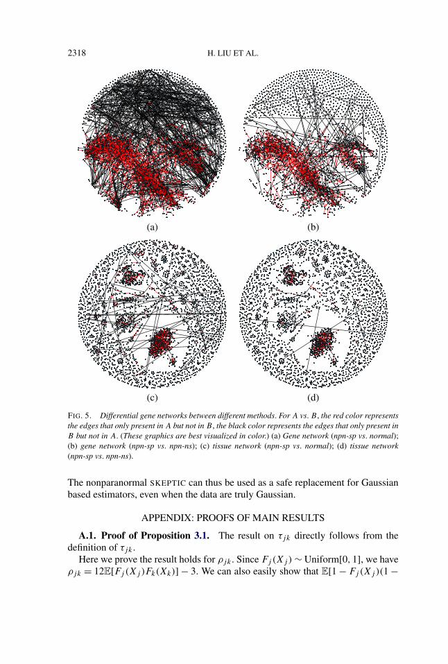
For example, at the gene level, the npn-sp graph contains 1235 edges that arenot in the normal graph. In contrast, the normal graph contains 1228 edges thatare not in the npn-sp graph. Since there are 1235/1557 ≈ 80% edges in npn-spthat are not present in the normal graph, this suggests that the data are highlynon-Gaussian. When we further compare the npn-sp gene graph with the npn-nsgraph, we found that there are 691/1557 ≈ 45% edges that are not present in thenpn-ns graph, suggesting that this data may contain high levels of outliers. Sincethis data set is integrated from many sources, this is not surprising. Comparedwith the gene graphs, the tissue graphs present a different pattern. Even thoughthe delivered tissue graphs are much denser than the gene graphs, there are only602/2714 ≈ 22% npn-sp edges that are not present in the normal graph. Also,there are only 342/2639 ≈ 12% edges in the normal graph that are not in the npn-sp graph. Such a result suggests that the data are still non-Gaussian. However, atthe tissue level the data seems to contain a much stronger signal than at the genelevel. (This may also be caused by possible uninterpreted lab effects.) A similarconclusion can be drawn when we compare the npn-spearman tissue graph withthe npn-ns tissue graph. For better visualization, we plot the differential graphsin Figure 5. These plots show the difference between the estimated graphs andconfirm the above analysis.

6. Conclusions and discussion. Most methods for estimating high-dimen-sional undirected graphs rely on the normality assumption. To weaken this overlyrestrictive parametric assumption, we propose the nonparanormal SKEPTIC. Thisimproved estimator obviates the need to explicitly estimate the marginal trans-formations and greatly improves the statistical rate of convergence. Our analysis isnonasymptotic, and the obtained rate is minimax optimal over many model classes.

2318 H. LIU ET AL.

(a) (b)

(c) (d)

FIG. 5. Differential gene networks between different methods. For A vs. B , the red color representsthe edges that only present in A but not in B , the black color represents the edges that only present inB but not in A. (These graphics are best visualized in color.) (a) Gene network (npn-sp vs. normal);(b) gene network (npn-sp vs. npn-ns); (c) tissue network (npn-sp vs. normal); (d) tissue network(npn-sp vs. npn-ns).

The nonparanormal SKEPTIC can thus be used as a safe replacement for Gaussianbased estimators, even when the data are truly Gaussian.

APPENDIX: PROOFS OF MAIN RESULTS

A.1. Proof of Proposition 3.1. The result on τjk directly follows from thedefinition of τjk .

Here we prove the result holds for ρjk . Since Fj (Xj ) ∼ Uniform[0,1], we haveρjk = 12E[Fj (Xj )Fk(Xk)] − 3. We can also easily show that E[1 − Fj (Xj )(1 −


Fk(Xk))] = E[Fj (Xj )Fk(Xk)]. Moreover, we have

E[Fj (Xj )Fk(Xk)

]= E

[P(X

(2)j < X

(1)j |X(1)

j

)P(X

(3)k < X

(1)k |X(1)

k

)](A.1)

= E[E(I(X

(2)j < X

(1)j ,X

(3)k < X

(k)j

) |X(1)j ,X

(1)k

)].

Similarly,

E[(

1 − Fj (Xj ))(

1 − Fk(Xk))]

= E[P(X

(2)j > X

(1)j |X(1)

j

)P(X

(3)k > X

(1)k |X(1)

k

)](A.2)

= E[E(I(X

(2)j > X

(1)j ,X

(3)k > X

(1)k

) |X(1)j ,X

(1)k

)].

Combining (A.1) and (A.2), we obtain

E[Fj (Xj )Fk(Xk)

]= 12E

[Fj (Xj )Fk(Xk)

]+ 12E

[(1 − Fj (Xj )

)(1 − Fk(Xk)

)]= 1

2P((

X(1)j − X

(2)j

)(X

(1)k − X

(3)k

)> 0

)= 1

2C(j,1,2;k,1,3).

Therefore, we have ρjk = 12E[Fj (Xj )Fk(Xk)]− 3 = 3(2C(j,1,2;k,1,3)− 1) =3C(j,1,2;k,1,3)−3D(j,1,2;k,1,3). The last equality follows from the fact thatC(j,1,2;k,1,3) = 1 − D(j,1,2;k,1,3).

A.2. Proof of Theorem 4.1. The main difficulty of this analysis is that Spear-man’s rho static is over rank variables which depend on all the samples. To handlethis issue, we first rewrite the rho-statistic in a different form [see page 318, Equa-tion (9.21) of Hoeffding (1948)]:

ρjk = 3

n3 − n

n∑i=1

n∑s=1

n∑t=1

sign(xij − xs

j

)(xik − xt

k

)= n − 2

n + 1Ujk + 3

n + 1τjk,

where τjk is Kenadall’s tau and Ujk = 3n(n−1)(n−2)

∑i �=s �=t sign(xi

j − xsj )(x

ik − xt

k)

is a 3rd-order U -statistic with bounded but asymmetric kernel.

Let 0 < α < 1. Since 6n+1 > 2

π(1 − α)c

√logd

nwhenever n ≥ 9π2

(1−α)2c2 logd, we

have

P

(supjk

|ρjk − Eρjk| > 2c

π

√logd

n

)≤ d2

P

(|Ujk − EUjk| > 2αc

π

√logd

n

)︸︷︷︸

T1(α)

.

2320 H. LIU ET AL.

Without loss of generality, we assume n can be divided by 3. Using Hoeffding’sinequality with asymmetric kernels [Hoeffding (1963)],

T1(α) = d2P

(|Ujk − EUjk| > 2αc

π

√logd

n

)

≤ 2d2 exp(− 2

9π2 α2c2⌊n

3

⌋· logd

n

)= 2 exp

(2 logd − 2

27π2 α2c2 logd

).

Let c = 3√

6πα

. Therefore, whenever n ≥ 16 logd

( α1−α

)2, with probability at least

1 − 2d−2, we have supjk |ρjk − Eρjk| ≤ 6√

6α

√logd

n.

Unlike τjk which is an unbiased estimator of τjk , ρjk is a biased estimator. Toprove the desired result, we apply the following bias equation from Zimmerman,Zumbo and Williams (2003):

Eρjk = 6

π(n + 1)

[arcsin

(�0

jk

)+ (n − 2) arcsin(�0

jk

2

)].

Equivalently, we can write

�0jk = 2 sin

(π

6Eρjk + ajk

)where ajk = πEρjk − 2 arcsin(�0

jk)

2(n − 2).

It is easy to see that |ajk| ≤ πn−2 . Therefore, for all n > 6π

t+ 2 (which implies that

|ajk| ≤ t6 ),

P

(supjk

∣∣Sρjk − �0

jk

∣∣> t)

= d2P

(∣∣∣∣2 sin(

π

6ρjk

)− 2 sin

(π

6Eρjk + ajk

)∣∣∣∣> t

)≤ d2

P

(∣∣∣∣ρjk − Eρjk − 6

πajk

∣∣∣∣> 3

πt

)≤ d2

P

(|ρjk − Eρjk| > 3

πt −

∣∣∣∣ 6

πajk

∣∣∣∣)≤ d2

P


πt − 1

πt

)= d2

P


πt

).

We get the desired result by choosing α = 3√

68 .


A.3. Proof of Theorem 4.2. It is easy to see that τjk is an unbiased estimatorof τjk : Eτjk = τjk . We have

P(∣∣Sτ

jk − �0jk

∣∣> t)= P

(∣∣∣∣sin(

π

2τjk

)− sin

(π

2τjk

)∣∣∣∣> t

)≤ P

(|τjk − τjk| > 2

πt

).

Since τjk can be written as a U -statistic, τjk = 2n(n−1)

∑1≤i<i′≤n Kτ (x

i, xi′),

where Kτ(xi, xi′) = sign(xi

j − xi′j )(xi

k − xi′k ) is a kernel bounded between −1

and 1. Using Hoeffding’s inequality for the U -statistic, we get

P

(supj,k

∣∣Sτjk − �0

jk

∣∣> t)

≤ d2 exp(− nt2

2π2

).

We then obtain (4.2).

A.4. Proof of Theorem 4.6. We first present some useful lemmas. Let �(·)and φ(·) be the cumulative distribution function and density function of standardGaussian. We start with some preliminary lemmas on the almost sure limit of theGaussian maxima and the standardized empirical processes. Since gj = f −1

j and

fj (t) = �−1(Fj (t)), we have gj (u) = F−1j (�(u)).

LEMMA A.1 [Pickands (1969)]. Letting z1, . . . , zn ∼ N(0,1), we then have

lim infn→∞sup1≤i≤n zi−√

2 logn

log logn/√

2 logn= −1

2 and lim supn→∞sup1≤i≤n zi−√

2 logn

log logn/√

2 logn= 1

2 al-

most surely.

For any γ > 0 and 0 < α < 1 < β ≤ 74(1 − γ ), we define subintervals

I1n := [gj (0), gj (√

α logn)] and I2n := [gj (√

α logn), gj (√

β logn)] and I3n :=[gj (

√β logn), gj (

√74(1 − γ ) logn)]. We also define

u∗n :=

√2 logn − log logn√

2 lognand t∗n :=

√2 logn + log logn√

2 logn.(A.3)

LEMMA A.2. For all t ∈ I1n ∪ I2n ∪ I3n, we have, for large enough n, 1n

≤Fj (t) ≤ 1 − 1

nalmost surely.

PROOF. By Lemma A.1, for any c > 0 and large enough n, we have the stan-dard Gaussian random variables z1, . . . , zn satisfy sup1≤i≤n zi ∈ [√2 logn − (1

2 +c)

log logn√2 logn

,√

2 logn + (12 + c)

log logn

2√

logn] almost surely. Letting c = 1

2 , we have, forlarge enough n,

P

(sup

1≤i≤n

zi ∈[√

2 logn − log logn√2 logn

,√

2 logn + log logn√2 logn

])= 1.

2322 H. LIU ET AL.

Using the definitions in (A.3), we have, for large enough n, sup1≤i≤n xij ∈

[gj (u∗n), gj (t

∗n)] almost surely. Therefore, sup1≤i≤n xi

j /∈ I1n ∪ I2n ∪ I3n al-

most surely. From the definition of Fj , only the values greater or equal to thesup1≤i≤n xi

j are truncated. The result then follows. �

The next lemma is from Chapter 16 of Shorack and Wellner (1986). It charac-terizes the almost sure limit of the standardized empirical process.

LEMMA A.3 (Almost sure limit of the standardized empirical process). Con-

sider a sequence of subintervals [L(j)n ,U

(j)n ] with both L

(j)n = gj (

√α logn) ↑ ∞

and U(j)n = gj (

√β logn) ↑ ∞, then for 0 < α < β ≤ 7

4(1 − γ )

lim supn→∞

√n

2 log lognsup

L(j)n <t<U

(j)n

∣∣∣∣ Fj (t) − Fj (t)√Fj (t)(1 − Fj (t))

∣∣∣∣= C a.s.,

where 0 < C ≤ 2√

2 is a constant.

PROOF. This result follows from a combination of Theorems 1 and 2 (Chap-ter 16) of Shorack and Wellner (1986). �

The following lemma characterizes the behavior of a random sequence using adeterministic sequence.

LEMMA A.4. For any 0 < α < 2, there exists a constant C, such that

lim supn→∞

(�−1)′(max{Fj (gj (√

α logn)),Fj (gj (√

α logn))})(�−1)′(Fj (gj (

√α logn)))

≤ C a.s.

PROOF. It suffices to consider the case Fj > Fj . First, for large enough n√φ(

√α logn)√

α logn≤ φ

(√α logn + 4

√log logn

n1−α/2

)· nα/4.(A.4)

This is true since φ(√

α logn + 4√

log logn

n1−α/2 ) = φ(√

α logn) · (1 − o(1)).Therefore,

φ

(√α logn + 4

√log logn

n1−α/2

)· nα/4 ≥ n−α/4

2√

π

and √φ(

√α logn)√

α logn= n−α/4

(2πα logn)1/4 .


Equation (A.4) follows from a combination of these results.Further, using the fact that 1 − �(t) ≤ φ(t)

tfor t ≥ 1, we have

4

√log logn

n

√1 − �(

√α logn)

≤ 4

√log logn

n

√φ(

√α logn)√

α logn

≤ 4 · φ(√

α logn + 4

√log logn

n1−α/2

)√log logn

n1−α/2

≤ �

(√α logn + 4

√log logn

n1−α/2

)− �(

√α logn),

where the last step follows from the mean value theorem.

Thus, �(√

α logn)+4√

log lognn

√1 − �(

√α logn) ≤ �(

√α logn+4

√log logn

n1−α/2 ).

By applying �−1(·) on both sides and the fact that Fj (gj (t)) = �(t), we have

�−1(Fj

(gj (

√α logn)

)+ 4

√log logn

n

√1 − Fj

(gj (

√α logn)

))

≤√

α logn + 4

√log logn

n1−α/2 .

From Lemma A.3, for large enough n, Fj (t) ≤ Fj (t) + 4√

log lognn

·√

1 − Fj (t).

Therefore, �−1(Fj (gj (√

α logn))) ≤ √α logn + 4

√log logn

n1−α/2 . Finally, we have(�−1)′(Fj

(gj (

√α logn)

))= 1

φ(�−1(Fj (gj (√

α logn))))

≤ √2π exp

((√

α logn + 4√

(log logn)/n1−α/2)2

2

)� (

�−1)′(Fj

(gj (

√α logn)

)).

This finishes the proof. �

PROOF OF THEOREM 4.6. Due to symmetricity, we only need to conduct

analysis on a subinterval of I sn ⊂ In : I s

n := [gj (0), gj (√

74(1 − γ ) logn)].

Recall that for any 0 < γ < 1 and 0 < α < 1 < β ≤ 74(1 − γ ), we de-

fine I1n := [gj (0), gj (√

α logn)] and I2n := [gj (√

α logn), gj (√

β logn)] and

2324 H. LIU ET AL.

I3n := [gj (√

β logn), gj (√

74(1 − γ ) logn)]. By Lemma A.2, we know that on

I1n ∪ I2n ∪ I3n, 1n

≤ Fj (t) ≤ 1 − 1n

for large enough n almost surely. Therefore, weonly need to analyze the term

supt∈I1n∪I2n∪I3n

∣∣�−1(Fj (t))− �−1(Fj (t)

)∣∣.We first consider the term supt∈I1n

|�−1(Fj (t)) − �−1(Fj (t))|. Since�−1 is a continuous function on the interval between min{Fj (gj (0)),Fj (gj (0))}and max{Fj (gj (

√α logn)),Fj (gj (

√α logn)} and is differentiable on the cor-

responding open set, by the mean-value theorem, for some ξn,t , such thatξn,t ∈ [min{Fj (gj (0)),Fj (gj (0))},max{Fj (gj (

√α logn)),Fj (gj (

√α logn))}].

Thus, |�−1(Fj (t)) − �−1(Fj (t))| = |(�−1)′(ξn,t )(Fj (t) − Fj (t))| for t ∈ I1n.By Lemma A.4, the following inequality holds almost surely:(

�−1)′(ξn,t ) ≤ (�−1)′(max

{Fj

(gj (

√α logn)

), Fj

(gj (

√α logn)

)})≤ C

(�−1)′(Fj

(gj (

√α logn)

))= C

φ(√

α logn)≤ c1n

α/2,

where C and c1 are some generic constants and φ(·) is the standard Gaussiandensity function.

Using |(�−1)′(ξn,t )| ≤ c1nα/2 and the Dvoretzky–Kiefer–Wolfowitz inequality,

we have supt∈I1n|�−1(Fj (t)) − �−1(Fj (t))| = OP (

√log logn

n1−α ). Next, we consider

the term supt∈I2n|�−1(Fj (t))−�−1(Fj (t))|. By Lemma A.3, for large enough n,

supt∈I2n

∣∣Fj (t) − Fj (t)∣∣= OP

(√log logn

n·√

1 − Fj

(gj (

√α logn)

))

= OP

(√log logn

n·√

n−α/2√

α logn

)

= OP

(√log logn

nα/2+1

).

Similarly, we have supt∈I2n|�−1(Fj (t)) − �−1(Fj (t))| = OP (

√log logn

n1+α/2−β ) and

supt∈I3n|�−1(Fj (t)) − �−1(Fj (t))| = OP (

√log logn

nβ/2−3/4+7γ /4 ). By choosing β =32(1 − γ ) and α = 1 − γ , all terms vanish. �

Acknowledgments. We thank David Donoho for constructive comments andhelpful discussions. We also thank Tuo Zhao for helpful discussions of this work.We are grateful to Professor Peter Bühlmann, the Associate Editor and the threereferees for their helpful comments and suggestions.


REFERENCES

BANERJEE, O., EL GHAOUI, L. and D’ASPREMONT, A. (2008). Model selection through sparsemaximum likelihood estimation for multivariate Gaussian or binary data. J. Mach. Learn. Res. 9485–516. MR2417243

CAI, T., LIU, W. and LUO, X. (2011). A constrained �1 minimization approach to sparse precisionmatrix estimation. J. Amer. Statist. Assoc. 106 594–607. MR2847973

CHRISTENSEN, D. (2005). Fast algorithms for the calculation of Kendall’s τ . Comput. Statist. 2051–62. MR2162534

DEMPSTER, A. P. (1972). Covariance selection. Biometrics 28 157–175.DRTON, M. and PERLMAN, M. D. (2007). Multiple testing and error control in Gaussian graphical

model selection. Statist. Sci. 22 430–449. MR2416818DRTON, M. and PERLMAN, M. D. (2008). A SINful approach to Gaussian graphical model selec-

tion. J. Statist. Plann. Inference 138 1179–1200. MR2416875FRIEDMAN, J. H., HASTIE, T. and TIBSHIRANI, R. (2008). Sparse inverse covariance estimation

with the graphical lasso. Biostatistics 9 432–441.HOEFFDING, W. (1948). A class of statistics with asymptotically normal distribution. Ann. Math.

Statist. 19 293–325. MR0026294HOEFFDING, W. (1963). Probability inequalities for sums of bounded random variables. J. Amer.

Statist. Assoc. 58 13–30. MR0144363JAMES, G. M., RADCHENKO, P. and LV, J. (2009). DASSO: Connections between the Dantzig

selector and lasso. J. R. Stat. Soc. Ser. B Stat. Methodol. 71 127–142. MR2655526KENDALL, M. (1948). Rank Correlation Methods. Griffin, London.KLAASSEN, C. A. J. and WELLNER, J. A. (1997). Efficient estimation in the bivariate normal

copula model: Normal margins are least favourable. Bernoulli 3 55–77. MR1466545KRUSKAL, W. H. (1958). Ordinal measures of association. J. Amer. Statist. Assoc. 53 814–861.

MR0100941LAFFERTY, J., LIU, H. and WASSERMAN, L. (2012). Sparse nonparametric graphical models.

Statist. Sci. To appear.LAM, C. and FAN, J. (2009). Sparsistency and rates of convergence in large covariance matrix

estimation. Ann. Statist. 37 4254–4278. MR2572459LEEK, J. T. and STOREY, J. D. (2007). Capturing heterogeneity in gene expression studies by sur-

rogate variable analysis. PLoS Genet. 3 e161.LIU, H., LAFFERTY, J. and WASSERMAN, L. (2008). Nonparametric regression and classification

with joint sparsity constraints. In Proceedings of the Twenty-Second Annual Conference on NeuralInformation Processing Systems (NIPS) 969–976. Curran Associates, Inc., Red Hook, NY.

LIU, H., LAFFERTY, J. and WASSERMAN, L. (2009). The nonparanormal: Semiparametric estima-tion of high dimensional undirected graphs. J. Mach. Learn. Res. 10 2295–2328. MR2563983

LIU, H., ROEDER, K. and WASSERMAN, L. (2010). Stability approach to regularization selection(StARS) for high dimensional graphical models. In Proceedings of the Twenty-Third Annual Con-ference on Neural Information Processing Systems (NIPS). Curran Associates, Inc., Red Hook,NY.

LIU, H. and ZHANG, J. (2009). Estimation consistency of the group lasso and its applications.J. Mach. Learn. Res. Proceedings Track 5 376–383.

LIU, H., CHEN, X., LAFFERTY, J. and WASSERMAN, L. (2010). Graph-valued regression. In Pro-ceedings of the Twenty-Third Annual Conference on Neural Information Processing Systems(NIPS). Curran Associates, Inc., Red Hook, NY.

LIU, H., XU, M., GU, H., GUPTA, A., LAFFERTY, J. and WASSERMAN, L. (2011). Forest densityestimation. J. Mach. Learn. Res. 12 907–951. MR2786914

MEINSHAUSEN, N. and BÜHLMANN, P. (2006). High-dimensional graphs and variable selectionwith the lasso. Ann. Statist. 34 1436–1462. MR2278363

http://www.ams.org/mathscinet-getitem?mr=2417243














2326 H. LIU ET AL.

PICKANDS, J. III (1969). An iterated logarithm law for the maximum in a stationary Gaussiansequence. Z. Wahrsch. Verw. Gebiete 12 344–353. MR0251776

RAVIKUMAR, P., WAINWRIGHT, M., RASKUTTI, G. and YU, B. (2009). Model selection in Gaus-sian graphical models: High-dimensional consistency of �1-regularized MLE. In Advances inNeural Information Processing Systems 22. MIT Press, Cambridge, MA.

RAVIKUMAR, P., LAFFERTY, J., LIU, H. and WASSERMAN, L. (2009). Sparse additive models. J. R.Stat. Soc. Ser. B Stat. Methodol. 71 1009–1030. MR2750255

ROTHMAN, A. J., BICKEL, P. J., LEVINA, E. and ZHU, J. (2008). Sparse permutation invariantcovariance estimation. Electron. J. Stat. 2 494–515. MR2417391

SHORACK, G. R. and WELLNER, J. A. (1986). Empirical Processes with Applications to Statistics.Wiley, New York. MR0838963

TSUKAHARA, H. (2005). Semiparametric estimation in copula models. Canad. J. Statist. 33 357–375. MR2193980

XUE, L. and ZOU, H. (2012). Regularized rank-based estimation of high-dimensional nonparanor-mal graphical models. Ann. Statist. To appear.

YUAN, M. (2010). High dimensional inverse covariance matrix estimation via linear programming.J. Mach. Learn. Res. 11 2261–2286. MR2719856

YUAN, M. and LIN, Y. (2007). Model selection and estimation in the Gaussian graphical model.Biometrika 94 19–35. MR2367824

ZIMMERMAN, D. W., ZUMBO, B. D. and WILLIAMS, R. H. (2003). Bias in estimation and hypoth-esis testing of correlation. Transformation 24 133–158.

H. LIU

DEPARTMENT OF OPERATIONS RESEARCH

AND FINANCIAL ENGINEERING

PRINCETON UNIVERSITY

PRINCETON, NEW JERSEY 08544USAE-MAIL: [email protected]

F. HAN

DEPARTMENT OF BIOSTATISTICS

BLOOMBERG SCHOOL OF PUBLIC HEALTH

JOHNS HOPKINS UNIVERSITY

BALTIMORE, MARYLAND 21205USAE-MAIL: [email protected]

M. YUAN

SCHOOL OF INDUSTRIAL AND SYSTEMS ENGINEERING

GEORGIA INSTITUTE OF TECHNOLOGY

NW ATLANTA, GEORGIA 30332USAE-MAIL: [email protected]

J. LAFFERTY

DEPARTMENT OF STATISTICS

UNIVERSITY OF CHICAGO

CHICAGO, ILLINOIS 60637USAE-MAIL: [email protected]

L. WASSERMAN

DEPARTMENT OF STATISTICS

CARNEGIE MELLON UNIVERSITY

PITTSBURGH, PENNSYLVANIA 15213USAE-MAIL: [email protected]








mailto:[email protected]





High-dimensional semiparametric Gaussian copula graphical...

Documents

Transcript of High-dimensional semiparametric Gaussian copula graphical...