Journal of Machine Learning Research 21 (2020) 1-24 Submitted 5/19, Revised 12/19; Published 5/20

High-dimensional Linear Discriminant Analysis Classifier forSpiked Covariance Model ∗

Houssem Sifaou houssem.sifaou@kaust.edu.sa

Abla Kammoun abla.kammoun@kaust.edu.sa

Mohamed-Slim Alouini slim.alouini@kaust.edu.sa

Computer, Electrical and Mathematical Science and Engineering Division,

King Abdullah University of Science and Technology (KAUST), Thuwal, KSA

Editor: Rina Foygel Barber

Abstract

Linear discriminant analysis (LDA) is a popular classifier that is built on the assumptionof common population covariance matrix across classes. The performance of LDA dependsheavily on the quality of estimating the mean vectors and the population covariance ma-trix. This issue becomes more challenging in high-dimensional settings where the numberof features is of the same order as the number of training samples. Several techniques forestimating the covariance matrix can be found in the literature. One of the most popularapproaches are estimators based on using a regularized sample covariance matrix, givingthe name regularized LDA (R-LDA) to the corresponding classifier. These estimators areknown to be more resilient to the sample noise than the traditional sample covariance ma-trix estimator. However, the main challenge of the regularization approach is the choiceof the optimal regularization parameter, as an arbitrary choice could lead to severe degra-dation of the classifier performance. In this work, we propose an improved LDA classifierbased on the assumption that the covariance matrix follows a spiked covariance model. Themain principle of our proposed technique is the design of a parametrized inverse covariancematrix estimator, the parameters of which are shown to be easily optimized. Numericalsimulations, using both real and synthetic data, show that the proposed classifier yieldsbetter classification performance than the classical R-LDA while requiring lower computa-tional complexity.

Keywords: Linear Discriminant Analysis, Spiked Covariance Models, High-DimensionalData, Random Matrix Theory.

1. Introduction

Linear Discriminant Analysis (LDA) based classifiers, originally proposed by R. A. Fisher(Fisher, 1936), are among the simplest algorithms used for classification tasks. Grounded inthe use of the maximum likelihood principle, LDA turns out to be the optimal classifier thatachieves the lowest misclassification rate under the assumption that the data is Gaussianwith perfectly known statistics, and common covariance matrix across classes (Hastie et al.,2001). However, in practice, the population covariance matrix and means associated with

∗. This work was funded by the office of sponsored research at KAUST. Part of the results in this paperhas been presented at the IEEE International Workshop on Signal Processing Advances in WirelessCommunications, 2018.

c©2020 Houssem Sifaou, Abla Kammoun, and Mohamed-Slim Alouini.

License: CC-BY 4.0, see https://creativecommons.org/licenses/by/4.0/. Attribution requirements are providedat http://jmlr.org/papers/v21/19-428.html.

Sifaou, Kammoun, and Alouini

each class could not be perfectly known. It is common practice to replace them in thediscriminant score of the LDA by the sample estimates computed based on the trainingdata. This should not affect severely the performance if the number of training samplesis sufficiently large compared to the number of features. However, in high-dimensionalsettings, the estimation of the covariance matrix and the means associated with each classis highly inaccurate, causing a severe degradation in the classification performance. Theimpact of the estimation noise has been discussed in (Fan and Fan, 2008) and a solutionbased on feature selection has been proposed. In some extreme situations in which thesample size is lower than the number of features, the use of the sample covariance matrix asa plug-in estimator is not allowed, as the discriminant score of the LDA involves computingthe inverse of the covariance matrix.

One popular attempt to solve all these issues is to use the regularized sample covariancematrices as a plug-in estimator of the population covariance matrix. The resulting clas-sifier is known as Regularized LDA (R-LDA) in reference to the regularization parameterin use. However, the choice of the regularization parameter is critical to achieving goodperformance. Several works propose to choose the regularization parameter as the optimalvalue that minimizes the misclassification rate, an approximation of which can be derivedusing recent results from random matrix theory (Zollanvari and Dougherty, 2015; Bakirovet al., 2016; Elkhalil et al., 2017a). However, this approach presents two major drawbacks.First, the estimation of the optimal regularization parameter is computationally expensive.Second, it does not take advantage of available prior information on the structure of thecovariance matrix.

In this paper, we propose, a novel approach based on the assumption that the pop-ulation covariance matrix is isotropic except for a finite number of symmetry breakingdirections (Hoyle and Rattray, 2003; Reimann et al., 1996). Such a model, known as spiked-model covariance matrix, has been used in many real applications including detection (Zhaoet al., 1986), EEG signals (Davidson, 2009; Fazli et al., 2011) and financial econometrics(Passemier et al., 2017; Kritchman and Nadler, 2008). Based on this model, we propose toconsider a class of sample covariance matrix estimators that follow the same spiked model,that is they can be written as a finite rank perturbation of a scaled identity matrix. Thedirections of the low-rank perturbation are given by the principal eigenvectors of the samplecovariance matrix, while its eigenvalues are some design parameters that are chosen so thatan approximation of the misclassification rate rate is minimized. Such an approximation iscomputed based on results from random matrix theory.

Interestingly, the optimal parameters are obtained in closed form, avoiding the need forusing the standard cross-validation approach. Compared to the classical R-LDA, the pro-posed classifier constitutes a novel improved LDA classifier, which we refer to as ”I-LDA”,that presents a lower complexity and a higher classification performance. The reductionin the computational cost is achieved since, unlike the R-LDA which requires the use ofa grid search to optimize the regularization parameter (Hastie et al., 2001; Bishop, 2006;Zollanvari and Dougherty, 2015; Elkhalil et al., 2017a) the optimal hyper-parameters of ourproposed classifier admit closed-form expressions that depend only on the training data. Wealso show that not only the proposed classifier outperforms R-LDA but also other popularclassification techniques such as support vector machine (SVM) and k-nearest neighbors(KNN).

2

High-dimensional LDA for Spiked Covariance Model

We also show that further improvement in the case of imbalanced classes can be obtainedby optimizing the intercept of the proposed classifier. This improvement is shown to besignificant in such cases, as shown by a set of numerical simulations. Moreover, extensionof the multi-class classification is discussed in section 3.4.

The main literature in relation to this work is represented by the works of Donoho etal. in (Donoho and Ghorbani, 2018; Donoho et al., 2018) which consider the problem ofcovariance matrix estimation under the assumption of a spiked covariance matrix model.However, in contrast to our work, the aforementioned papers consider generic loss functionsthat are not directly related to the objective of interest which is herein the misclassificationrate. Specifically, (Donoho and Ghorbani, 2018) considers the design of the optimal shrink-age that optimizes a condition number loss function while (Donoho et al., 2018) examinesthe optimization of 26 loss functions. As evidenced later through numerical simulations insection 4, as far as LDA classification is considered, the proposed classifier yields betterperformance. Under the setting of incomplete data, the problem of high-dimensional LDAhas also been considered through the prism of optimality theory in (Cai and Zhang, 2019)where a classification algorithm based on an adaptive constrained `1 minimization approachhas been proposed and compared with (Shao et al., 2011).

The rest of the paper is organized a follows. In the next section, we give a brief overviewof LDA and R-LDA classifiers. In section 3, the steps of designing the proposed classifierare detailed. The performance of our technique is studied in section 4 using numericalsimulations before concluding in section 5.

Throughout this work, boldface lower case is used for denoting column vectors, x, andupper case for matrices, X. XT denotes the transpose. Moreover, Ip denotes the p × pidentity matrix and ‖.‖ is used to denote the `2-norm for vectors and spectral norm formatrices. The notation

a.s.−→ is used for the almost sure convergence of sequence of randomvariables. The trace of a matrix A is denoted by tr A and diag(x1, · · · , xn) stands for thediagonal matrix with diagonal entries x1, · · · , xn. The notation f(x) = O(g(x)) means that

|f(x)g(x) | is bounded as x −→∞.

2. Linear Discriminant Analysis

Consider a set of n vector observations x1, · · · ,xn in Rp×1 belonging to two classes C0 andC1. For i ∈ {0, 1}, we denote by ni the number of observations in Ci and by Ti the setof their indexes. Moreover, all observations are assumed to be independent and drawnfrom a Gaussian mixture model in which both classes have different means but a commoncovariance matrix. In particular, for i ∈ {0, 1},

xi ∈ Ci ⇔ xi ∼ N (µi,Σ),

where µi and Σ are respectively the mean vector and the covariance matrix associated withclass Ci. We assume that the class labels associated with vector observations {x`}n`=1 areperfectly known. These observations constitute the training sample that is used to build aclassifier, the aim of which is to predict the class label of an unseen observation x.

For the reader convenience, we start by presenting the classical LDA classifier. Its corre-sponding discriminant score is (Hastie et al., 2001; Bishop, 2006; Zollanvari and Dougherty,

3

Sifaou, Kammoun, and Alouini

2015):

WLDA(x) =

(x− µ0 + µ1

2

)TΣ−1(µ0 − µ1)− log

π1π0, (1)

where πi is the prior probability corresponding to class i. The unseen observation x isassigned to class C0 if WLDA(x) > 0 and to class C1 otherwise. In practice, the classstatistics namely its mean vector and covariance matrix are unknown. They are usuallyestimated from training data using the empirical means xi and the pooled sample covariancematrix Σ defined as:

µi = xi =1

ni

∑`∈Ti

x`, (2)

Σ =(n0 − 1)Σ0 + (n1 − 1)Σ1

n− 2, (3)

where

Σi =1

ni − 1

∑`∈Ti

(x` − xi)(x` − xi)T , i = 0, 1.

with ni is the number of observations belonging to class Ci and Ti is the set of indexesof observations belonging to class Ci. Replacing µi and Σ by their estimates yields thefollowing LDA discriminant rule:

WLDA(x) =

(x− x0 + x1

2

)TΣ−1

(x0 − x1)− logπ1π0. (4)

In the case where the size of the observations p is higher than the number of availabletraining samples n, Σ is singular. One popular solution consists in using ridge estimatorsof the inverse covariance matrix (Hastie et al., 2001; Zollanvari and Dougherty, 2015):

H =(Ip + γΣ

)−1, γ > 0. (5)

as a plug-in estimator of the inverse of the covariance matrix. The corresponding dis-criminant score is known as regularized LDA (R-LDA) in reference to the regularizationparameter γ and is given by:

WR−LDA(x) =

(x− x0 + x1

2

)TH(x0 − x1)− log

π1π0. (6)

Conditioning on the training samples, the discriminant score WLDA(x) is Gaussian in x. Inlight of this observation, the conditional misclassification rate associated with class Ci canbe expressed as:

εLDAi = Φ

(−1)i+1G(µi,x0,x1, Σ) + (−1)i log π1π0√

D(x0,x1, Σ,Σ)

, (7)

4

High-dimensional LDA for Spiked Covariance Model

where Φ(.) is the cumulative distribution function of a standard normal random variableand

G(µi,x0,x1, Σ) =

(µi −

x0 + x1

2

)Σ−1

(x0 − x1),

D(x0,x1, Σ,Σ) = (x0 − x1)T Σ−1

ΣΣ−1

(x0 − x1).

The total misclassification rate can be expressed as:

εLDA = π0εLDA0 + π1ε

LDA1 . (8)

Along the same arguments, the misclassification rate associated with R-LDA takes the same

expression with Σ−1

being replaced by H in (8). The resulting expression cannot provideinsights into how the theoretical mean and covariance of each class impact the classificationperformances. Such information is critical to properly choose the regularization parameter.

One approach to get around this issue is to use asymptotic results from random matrixtheory which lead to approximate the quantities G(µi,x0,x1, Σ) and D(x0,x1, Σ,Σ) bydeterministic equivalents that solely involve {µi}

2i=1 and Σ (Zollanvari and Dougherty, 2015;

Elkhalil et al., 2017b; Dobriban and Wager, 2018). An approximation of the classificationperformance is thus obtained by replacing G(µi,x0,x1, Σ) and D(x0,x1, Σ,Σ) with theirdeterministic equivalents in (8). Such an approximation cannot still be directly used tooptimize the regularization parameter since it depends on the unknown covariance matrix Σand {µi}

1i=0. The works in (Zollanvari and Dougherty, 2015; Elkhalil et al., 2017b) proposes

consistent estimates of the misclassification rates, which were then optimized through a gridsearch.

This approach has been shown through simulations to outperform the classical cross-validation technique used often for the setting of the regularization parameter. It howeverpresents two major drawbacks. First, the optimization of the regularization parameterinvolves a grid-search procedure which can lead to prohibitively high computational costswhen high dimension settings are considered. Second, it uses the sample covariance matrixas a plug-in estimator of the covariance matrix. Such an estimator is no longer consistentwhen the number of samples is comparable with that of features, which leads to highestimation noises and in turn to low classification performances.

In this paper, we propose an improved LDA classifier that overcomes both drawbacksand that is particularly suitable in scenarios wherein Σ takes the following particular form(Hoyle and Rattray, 2003; Reimann et al., 1996):

Σ = σ2Ip + σ2r∑j=1

λjvjvTj , (9)

where σ2 > 0, λ1 ≥ · · · ,≥ λr > 0 and v1, · · · ,vr are orthonormal. The above model isencountered in many real applications, among which detection (Zhao et al., 1986), EEGsignals (Davidson, 2009; Fazli et al., 2011) and financial econometrics (Passemier et al.,2017; Kritchman and Nadler, 2008) are the best representatives. The design of the improvedclassifier will be detailed in the next section.

5

Sifaou, Kammoun, and Alouini

3. Improved LDA

3.1. Proposed estimation approach

In this section, we present our improved LDA classifier, which unlike the traditional R-LDA,leverages the particular finite rank perturbation property of the true covariance matrix.For the sake of simplicity, we assume that σ2 and r are perfectly known. In practice, onecan resort to the existing efficient algorithms available in the literature for the estimationof these parameters. We refer the reader to the following works and the references therein(Kritchman and Nadler, 2008; Johnstone and Lu, 2009; Ulfarsson and Solo, 2008; Passemieret al., 2017). In our numerical simulations, we have used the method of (Ulfarsson and Solo,2008). Starting from the eigen decomposition of the pooled covariance matrix:

Σ =

p∑j=1

sjujuTj ,

with sj being the j-th largest eigenvalue and uj its corresponding eigenvector, and notingthat:

Σ−1 =1

σ2

Ip −r∑j=1

λj1 + λj

vjvTj

, (10)

it is sensible to seek for estimators of Σ−1 that takes the form:

C−1 =1

σ2

Ip +

r∑j=1

wjujuTj

, (11)

where {wj}rj=1 are some design parameters to be optimized. We assume that wj ∈ R =[−1 + ζ, χ) for some 0 < ζ < 1 and χ > 1. From a practical point of view, we only need toassume that wj > −1 to ensure that C−1 is positive definite. However, the restriction tothe range R is needed later for the proof of the uniform convergence results. Plugging (11)

in place of Σ−1

into (1), yields the following discriminant score:

W I−LDA =

(x− x0 + x1

2

)TC−1(x0 − x1)− log

π1π0. (12)

It is worth mentioning that the estimator C−1 can be seen as an instance of the wider classof estimators taking the form

∑pj=1 ηjuju

Tj , where uj being the eigenvector of the sample

covariance matrix associated with its j-th largest eigenvalue and scalars ηj are referred toas shrinkage functions that need to be designed (Daniels and Kass, 2001; Ledoit and Wolf,2004; Karoui, 2018; Chen et al., 2010; Ledoit and Wolf, 2017). Indeed, C−1 is obtained bysetting ηr+1 = . . . = ηp = 1

σ2 and wj = σ2ηj − 1. The main challenge is how to select theappropriate values of the design parameters wj .

3.2. Parameter optimization

Given the application into consideration, it is sensible to select the wj so that they minimizethe total misclassification rate:

w? = argminw

εI−LDA(w), (13)

6

High-dimensional LDA for Spiked Covariance Model

where w = [w1, · · · , wr]T and εI−LDA(w) is obtained by replacing Σ−1

by C−1 in (8).Finding the optimal w that exactly solves (13) could not be in general obtained. To

get around this problem, we invoke results from random matrix theory that approximatethe total misclassification rate under the asymptotic growth regime defined in the followingassumption.

Assumption 1 Throughout this work, we assume that

(i) n, p −→∞, with fixed ratio c = p/n.

(ii) n0, n1,−→∞, with p/n0 , c0, p/n1 , c1 where c0 and c1 are fixed constants.

(iii) r is fixed and λ1 > · · · > λr >√c, independently of p and n.

(iv) The mean difference vector µ , µ1 − µ0 has a bounded Euclidean norm, that is‖µ‖ = O(1).

(v) The spectral norm of Σ is bounded, that is ‖Σ‖ = O(1).

Remark 1 • Assumptions (i), (ii) and (iii) are key assumptions that are generally usedin the framework of the theory of large random matrices.

• Assumption (iii) is fundamental in our analysis since it guarantees, as per standardresults from random matrix theory, the one-to-one mapping between the sample eigen-values sj and the unknown λj. In fact, when λj >

√c, λj can be consistently estimated

using its corresponding sj as we will see later. In the case where λj ≤√c, the relation

between sj and λj no longer holds and λj cannot be estimated (Couillet and Debbah,2011; Baik et al., 2005).

• Assumption (iv) controls the order of the euclidean norm of µ that ensures asymptot-ically non-trivial classification.

It should be noted that from a methodological perspective, the approach undertaken in thiswork that consists in optimizing a loss function for a spiked covariance model is similar tothe one introduced earlier in (Donoho et al., 2018). It basically consists in computing anasymptotic approximation for the considered loss function based on the asymptotics of theeigenvalues and eigenvectors of the spiked model characterized in (Baik et al., 2005) and(Paul, 2007) and then optimizing the parameters that optimize this approximation. How-ever, the main difference with the approach of (Donoho et al., 2018) is that the consideredloss function is relevant to the underlying application. In doing so, better performances areexpected compared to the approach that considers generic loss functions. Depending on thescenario into consideration, different loss functions can be considered, including the SharpRatio in the context of Markowitz portfolio allocation or the SNR in the context the designof MVDR beamforming, as examined in (Yang et al., 2018).

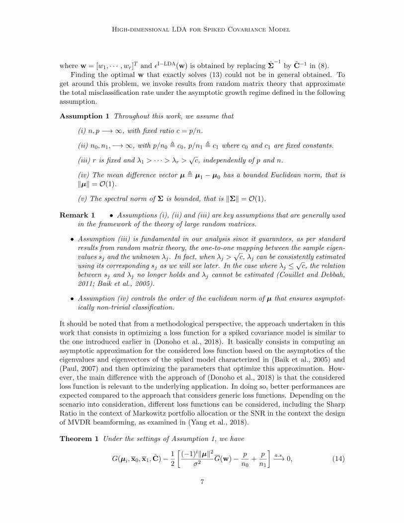
Theorem 1 Under the settings of Assumption 1, we have

G(µi,x0,x1, C)− 1

2

[(−1)i‖µ‖2

σ2G(w)− p

n0+

p

n1

]a.s.−→ 0, (14)

7

Sifaou, Kammoun, and Alouini

D(x0,x1, C,Σ)−[‖µ‖2

σ2D(w) +

p

n0+

p

n1

]a.s.−→ 0, (15)

where

G(w) = 1 +

r∑j=1

ajbjwj ,

D(w) = 1 +r∑j=1

[λjbj + 2ajbj(λj + 1)wj ] +r∑j=1

[ajbj(1 + λjaj)w

2j

],

with

µ = µ0 − µ1, aj =1− c/λ2j1 + c/λj

, bj =µTvjv

Tj µ

‖µ‖2, j = 1, · · · , r (16)

Proof See Appendix A.

Using these deterministic equivalents and after some manipulations, a deterministic equiv-alent of the global misclassification rate can be obtained as:

εI−LDA(w)− εI−LDA(w)a.s.−→ 0.

where

εI−LDA(w) = π0Φ

−√α(G(w)− η)

2√D(w) + κ

+ π1Φ

−√α(G(w) + η)

2√D(w) + κ

(17)

with α = ‖µ‖2σ2 , η = 1

α [c/π0−c/π1+2 log π1π0

] and κ = 1α [p/n0+p/n1]. In order to ensure that

the this convergence result is guaranteed at optimality, we need to establish the uniformconvergence of εI−LDA(w). This is the objective of the following theorem.

Theorem 2 Under the settings of Assumption 1, we have

supw∈Rr

|εI−LDA(w)− εI−LDA(w)| a.s.−→ 0.

where εI−LDA(w) is given in (17).

Proof See Appendix D

Now, with the asymptotic equivalent of the misclassification rate on hand, we can determinethe optimal parameters w?j .

Theorem 3 Under the settings of Assumption 1, the optimal parameters {w?j} that mini-

mize εI−LDA(w) are given by:

w?j =u?

β

γjαj− βj , j = 1, · · · , r (18)

8

High-dimensional LDA for Spiked Covariance Model

where

αj = λja2jbj + ajbj , βj =

λj + 1

λjaj + 1, γj = ajbj , j = 1, ..., r,

β =√∑r

j=1 γ2j /αj, and u? is the minimizer of the scalar function g(u) given by

g(u) = π0Φ

(−√α

2

βu+ d0√u2 + b

)+ π1Φ

(−√α

2

βu+ d1√u2 + b

),

with

b = 1 + κ+

r∑j=1

[λjbj −

(λjajbj + ajbj)2

λja2jbj + ajbj

], (19)

d0 = 1− η −r∑j=1

λjajbj + ajbjλjaj + 1

, (20)

d1 = 1 + η −r∑j=1

λjajbj + ajbjλjaj + 1

. (21)

Proof See Appendix B.

Remark 2 In the case of equiprobable classes, u? can be computed in closed formexpression as u? = βb

d , where d = d0+d12 = 1−

∑rj=1

λjajbj+ajbjλjaj+1 .

3.3. Improved LDA with optimal intercept

Bias correction is a general procedure that aims to optimize the bias in the discriminantscore of a given classifier to minimize the misclassification rate. It has been considered inseveral previous works; see for instance (Chan and Peter, 2009) and (Huang et al., 2010)and the references therein, and has been recently applied to LDA and R-LDA in (Cheng andBinyan, 2018). Generally, bias correction allows to bring a gain in performance especiallyin high-dimensional settings and imbalanced classes. This is because the original bias inLDA, introduced essentially to calibrate the case of unequal sample sizes across classes, isdevised under the assumption that the sample size is sufficiently high. There is thus roomfor further improvement to adapt this bias to high-dimensional settings. Following this lineof ideas, we apply the bias correction procedure to the improved LDA classifier and showthat not only the optimization of the parameters get simplified but also a significant gain isobtained once the bias is optimally set. The resulting classifier will be named as ”OII-LDA”in reference to optimal-intercept-improved-LDA. Starting off from our proposed classifierclassifier and replacing the constant term with a parameter θ, the score function can bewritten as:

WOII−LDA =

(x− x0 + x1

2

)TC−1(x0 − x1) + θ,

9

Sifaou, Kammoun, and Alouini

where θ is a parameter that will be optimized. The corresponding misclassification rate canbe expressed in this case as,

εOII−LDA = π0Φ

−G(µ0,x0,x1, C)− θ√D(x0,x1, C,Σ)

+ π1Φ

G(µ1,x0,x1, C) + θ√D(x0,x1, C,Σ)

.Following similar steps as in the previous section, the asymptotic equivalent of εOII−LDA

can be obtained as for εI−LDA:

εOII−LDA − εOII−LDA a.s.−→ 0.

where

εOII−LDA =π0Φ

−√α[G(w)− 1

α

(pn0− p

n1− 2θ

)]2√D(w) + κ

+π1Φ

−√α[G(w) + 1

α

(pn0− p

n1− 2θ

)]2√D(w) + κ

Taking the derivative of εOII−LDA and equating it to zero yields the optimal θ:

θ? =1

2

[p

n0− p

n1

]− D(w) + κ

G(w)log

π1

π0

Replacing θ? by its expression, the asymptotic misclassification rate becomes

εOII−LDA =π0Φ

−√αG(w)

2√D(w) + κ

+

√D(w) + κ√αG(w)

logπ1

π0

+π1Φ

−√αG(w)

2√D(w) + κ

−

√D(w) + κ√αG(w)

logπ1

π0

(22)

Now, we are able to find the new optimal parameter vector w that minimizes the asymptoticmisclassification rate εOII−LDA.

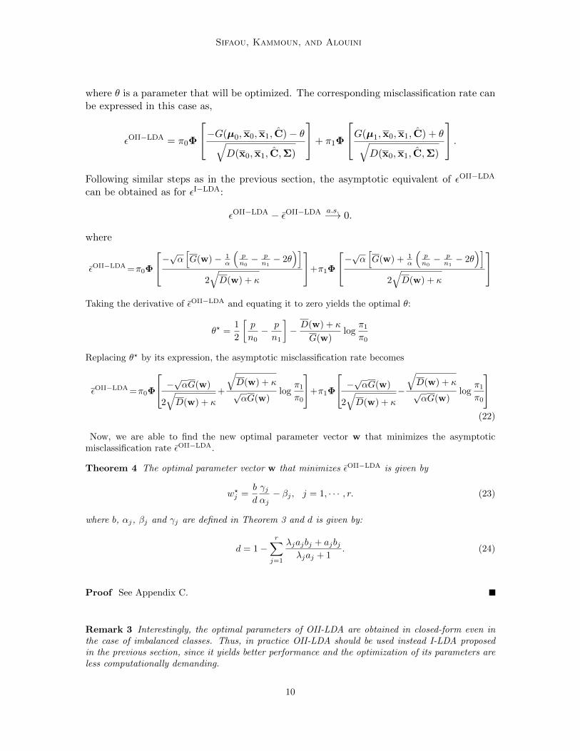
Theorem 4 The optimal parameter vector w that minimizes εOII−LDA is given by

w?j =b

d

γjαj− βj , j = 1, · · · , r. (23)

where b, αj, βj and γj are defined in Theorem 3 and d is given by:

d = 1−r∑j=1

λjajbj + ajbjλjaj + 1

. (24)

Proof See Appendix C.

Remark 3 Interestingly, the optimal parameters of OII-LDA are obtained in closed-form even inthe case of imbalanced classes. Thus, in practice OII-LDA should be used instead I-LDA proposedin the previous section, since it yields better performance and the optimization of its parameters areless computationally demanding.

10

High-dimensional LDA for Spiked Covariance Model

The optimal design parameters in Theorems 3 and 4 could not be directly used in practice, sincethey depend on the unobservable quantities λj and bj . To solve this issue, consistent estimators forthese quantities need to be retrieved. This is the objective of the following result:

Proposition 5 Under the settings of Assumption 1, we have

|α− α| a.s.−→ 0, |λj − λj |a.s.−→ 0, and |bj − bj |

a.s.−→ 0,

where

α =‖µ‖2

σ2− c1 − c0

λj =sj/σ

2 + 1− c+√

(sj/σ2 + 1− c)2 − 4sj/σ2

2− 1,

bj =1 + c/λj

1− c/λ2j

µTujuTj µ

‖µ‖2 − c1σ2 − c0σ2, j = 1, · · · , r.

with c0 = pn0 , c1 = p

n1 , µ = x0 − x1, and sj is the j-th largest eigenvalue of the pooled covariancematrix.

Proof The proof is a direct application of results from (Couillet and Debbah, 2011, Theorem 9.1and Theorem 9.9) and it is thus omitted.

Replacing α, λj and bj by their estimates yields a consistent estimator w?j of w?j . Even though we haveassumed that the data follow a Gaussian distribution, our results hold for non-Gaussian data undersome moment assumptions on the entries. This is due to the fact that all the results regarding thecovariance spiked model were proven for non-Gaussian data in (Benaych-Georges and Nadakuditi,2011). Moreover, the optimal parameters of our proposed classifier OII-LDA, are independent of thespecific distribution, that is, replacing Φ with other cumulative distribution function will not affectthe expressions of the optimal parameters in (23).

3.4. Extension to multi-class classification

The proposed binary classifier can be easily extended to the case of multi-class classification. In themachine learning literature, this can be performed by combining the use of multiple binary classifiersto devise a multi-class classifier. Two popular methods have been proposed towards this aim. Theseare commonly known as One vs. Rest and One vs. One approaches Assume that the total number ofclasses is C. The one vs the rest approach consists in training one binary classifier for each class byconsidering the rest of the classes as forming one class. Then, the output of these C binary classifiersare combined to decide the class of the unseen observation x. On the other hand, the one vs oneconsists in training C(C−1)/2 binary classifiers corresponding to each possible pair of classes. Then,the output of these binary classifiers are combined to predict the class of the unseen observation x.In our case and this also holds for R-LDA, the one vs the rest approach is not applicable since theclass formed by the remaining observations from the C − 1 classes is not homogeneous in the sensethat it is formed by observations drawn from a mixture of Gaussian distribution rather than froma Gaussian distribution as required by our results. However, the second approach (one vs. one) isapplicable in our case and should allow extending our binary classifier to the multi-class classificationcase. As already known, the one vs one approach may lead to ambiguities (Bishop, 2006) as someclasses may receive the same number of votes. This issue can be solved by giving priority to thedecision with the highest scores.

11

Sifaou, Kammoun, and Alouini

4. Numerical Simulations

In this section, we study the performance of the proposed improved LDA classifier. We compare itsperformance with R-LDA classifier and other classical classifiers based on both synthetic and realdata.

4.1. Synthetic data

In the synthetic data simulations, we use the following Monte Carlo protocol to estimate the truemisclassification rate:

• Step 1: Set σ2 = 1 and choose r = 3 orthogonal symmetry breaking directions as follows: v1 = [1, 0, · · · , 0]T , v2 = [0, 1, 0, · · · , 0]T , v3 = [0, 0, 1, 0 · · · , 0]T and their correspondingweights λ1 = 8, λ2 = 7, λ3 = 6. Set µ0 = 1√

p [a, a, · · · , a]T and µ1 = −µ0 where a is a finite

constant. We choose a = 2 and a = 2.5.

• Step 2: Generate ni training samples for class i.

• Step 3: Using the training set, design the improved LDA classifier as explained in section 3and determine the optimal parameter γ∗ of R-LDA using grid search over γ ∈ {10i/10, i =−10 : 1 : 10}.

• Step 4: Estimate the misclassification rate of both classifiers using a set of 1000 testingsamples.

• Step 5: Repeat Step 2–4, 500 times and determine the average classification true error of bothclassifiers. In all figures, 95% confidence intervals are plotted along with the Monte Carloestimate of the misclassification rate.

In Fig. 1, we plot the misclassification rate vs. training sample size n when p = 150 and π0 = 0.2 forthe proposed improved LDA and the classical R-LDA using synthetic data. It is observed that theimproved LDA outperforms the classical R-LDA and the gap between the two schemes is significant.

100 120 140 160 180 2003

4

5

6

7·10−2

Sample size n

Mis

clas

sifica

tion

rate

R-LDAI-LDA

OII-LDA

(a) a = 2

100 120 140 160 180 200

1

1.5

2

2.5

·10−2

Sample size n

Mis

clas

sifica

tion

rate

R-LDAI-LDA

OII-LDA

(b) a = 2.5

Figure 1: Misclassification rate vs. sample size n for p = 150 and π0 = 0.2. Comparisonbetween Improved LDA and R-LDA with synthetic data.

12

High-dimensional LDA for Spiked Covariance Model

800 850 900 950 1,0002.6

2.7

2.8

2.9

3

3.1·10−2

Sample size n

Mis

clas

sifica

tion

rate

R-LDAOII-LDA

(a) Digits 3 and 8

800 850 900 950 1,0001.6

1.7

1.8

1.9

2·10−2

Sample size n

Mis

clas

sifica

tion

rate

R-LDAOII-LDA

(b) Digits 4 and 9

800 850 900 950 1,0001.1

1.2

1.3

1.4

1.5·10−2

Sample size n

Mis

clas

sifica

tion

rate

R-LDAOII-LDA

(c) Digits 8 and 9

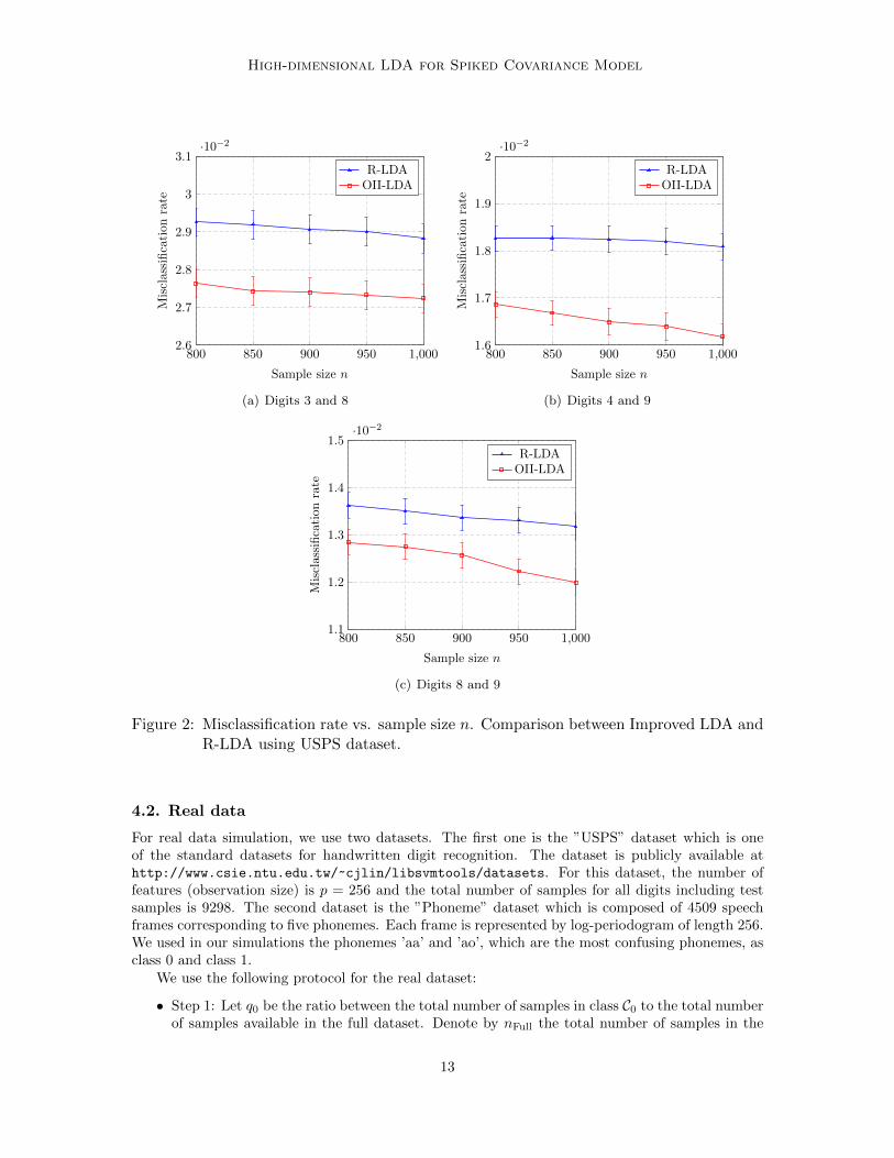
Figure 2: Misclassification rate vs. sample size n. Comparison between Improved LDA andR-LDA using USPS dataset.

4.2. Real data

For real data simulation, we use two datasets. The first one is the ”USPS” dataset which is oneof the standard datasets for handwritten digit recognition. The dataset is publicly available athttp://www.csie.ntu.edu.tw/~cjlin/libsvmtools/datasets. For this dataset, the number offeatures (observation size) is p = 256 and the total number of samples for all digits including testsamples is 9298. The second dataset is the ”Phoneme” dataset which is composed of 4509 speechframes corresponding to five phonemes. Each frame is represented by log-periodogram of length 256.We used in our simulations the phonemes ’aa’ and ’ao’, which are the most confusing phonemes, asclass 0 and class 1.

We use the following protocol for the real dataset:

• Step 1: Let q0 be the ratio between the total number of samples in class C0 to the total numberof samples available in the full dataset. Denote by nFull the total number of samples in the

13

Sifaou, Kammoun, and Alouini

full dataset. Choose n < nFull the number of training samples; set n0 = bq0nc, where b.c isthe floor function and n1 = n− n0. Take ni training samples belonging to class Ci randomlyfrom the full dataset. The remaining samples are used as a test dataset in order to estimatethe misclassification rate.

• Step 2: Using the training dataset, design the improved LDA classifier as explained in section3 and determine the optimal parameter γ∗ of R-LDA using grid search over γ ∈ {10i/10, i =−10 : 1 : 10}

• Step 3: Using the test dataset, estimate the true misclassification rate for both classifiers.

• Step 4: Repeat steps 1–4 500 times and determine the average misclassification rate of bothclassifiers.

In Fig. 2, the misclassification rate vs. training sample size is plotted for the R-LDA and ourproposed classifier. Three pairs of the most confusing digits are chosen for simulation; (3,8), (4,9)and (8,9). As seen, the performance of the proposed classifier is better than R-LDA classifier andthe gain is significant. For example, more that 10% gain in terms of misclassification rate is obtainedfor digits (4,9) when n = 1000.

600 700 800 900 1,000

0.18

0.2

0.22

0.24

Sample size n

Mis

clas

sifi

cati

on

rate

R-LDAOII-LDA

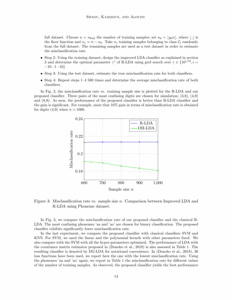
Figure 3: Misclassification rate vs. sample size n. Comparison between Improved LDA andR-LDA using Phoneme dataset.

In Fig. 3, we compare the misclassification rate of our proposed classifier and the classical R-LDA. The most confusing phonemes ’aa and ’ao’ are chosen for binary classification. The proposedclassifier exhibits significantly lower misclassification rate.

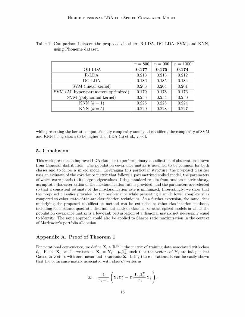
In the last experiment, we compare the proposed classifier with classical classifiers SVM andKNN. For SVM, we used the linear and the polynomial kernels with other parameters fixed. Wealso compare with the SVM with all the hyper-parameters optimized. The performance of LDA withthe covariance matrix estimator proposed in (Donoho et al., 2018) is also assessed in Table 1. Theresulting classifier is denoted by DG-LDA for notational convenience. In (Donoho et al., 2018), 26loss functions have been used, we report here the one with the lowest misclassification rate. Usingthe phonemes ’aa and ’ao’ again, we report in Table 1 the misclassification rate for different valuesof the number of training samples. As observed, the proposed classifier yields the best performance

14

High-dimensional LDA for Spiked Covariance Model

Table 1: Comparison between the proposed classifier, R-LDA, DG-LDA, SVM, and KNN,using Phoneme dataset.

n = 800 n = 900 n = 1000

OII-LDA 0.177 0.175 0.174

R-LDA 0.213 0.213 0.212

DG-LDA 0.186 0.185 0.184

SVM (linear kernel) 0.206 0.204 0.201

SVM (All hyper-parameters optimized) 0.179 0.178 0.176

SVM (polynomial kernel) 0.255 0.254 0.250

KNN (k = 1) 0.226 0.225 0.224

KNN (k = 5) 0.229 0.228 0.227

while presenting the lowest computationally complexity among all classifiers, the complexity of SVMand KNN being shown to be higher than LDA (Li et al., 2006).

5. Conclusion

This work presents an improved LDA classifier to perform binary classification of observations drawnfrom Gaussian distribution. The population covariance matrix is assumed to be common for bothclasses and to follow a spiked model. Leveraging this particular structure, the proposed classifieruses an estimate of the covariance matrix that follows a parametrized spiked model, the parametersof which corresponds to its largest eigenvalues. Using standard results from random matrix theory,asymptotic characterization of the misclassification rate is provided, and the parameters are selectedso that a consistent estimate of the misclassification rate is minimized. Interestingly, we show thatthe proposed classifier provides better performance while presenting a much lower complexity ascompared to other state-of-the-art classification techniques. As a further extension, the same ideasunderlying the proposed classification method can be extended to other classification methods,including for instance, quadratic discriminant analysis classifier or other spiked models in which thepopulation covariance matrix is a low-rank perturbation of a diagonal matrix not necessarily equalto identity. The same approach could also be applied to Sharpe ratio maximization in the contextof Markowitz’s portfolio allocation.

Appendix A. Proof of Theorem 1

For notational convenience, we define Xi ∈ Rp×ni the matrix of training data associated with classCi. Hence Xi can be written as Xi = Yi + µi1

Tni such that the vectors of Yi are independent

Gaussian vectors with zero mean and covariance Σ. Using these notations, it can be easily shownthat the covariance matrix associated with class Ci writes as

Σi =1

ni − 1

(YiY

Ti −Yi

1ni1Tni

niYTi

).

15

Sifaou, Kammoun, and Alouini

Let1ni1

Tni

ni= OiEiO

Ti , the eigenvalue decomposition of

1ni1Tni

ni, with Ei = diag

([1,0(ni−1)×1]

)and

Oi ∈ Rni×ni orthogonal matrix whose first column is 1√ni

1ni . Define Yi = YiOi. Thus, we have

Σi =1

ni − 1

(YiOiO

Ti YT

i −YiOiEiOTi YT

i

),=

1

ni − 1

(YiY

Ti − yi,1y

Ti,1

),

where yi,1 is the first column of Yi. Let Yi be Yi with the first column removed. Due to the

invariance of Gaussian distribution under orthogonal transformation, the columns of Yi follow aGaussian distribution with mean 0 and covariance Σ. The pooled covariance matrix given by

Σ =1

n− 2

((n0 − 1)Y0Y

T

0 + (n1 − 1)Y1Y1

), (25)

follow a standard spiked model for which standard results from random matrix theory apply. In thisrespect, we have the following results from (Couillet and Debbah, 2011)

vTj ukuTk vj − ajδj,k

a.s.−→ 0, k = 1, . . . , r (26)

1

‖µ‖2µTuju

Tj µ− ajbj

a.s.−→ 0, j = 1, · · · , r

where δj,k denotes the Kronecker delta and aj and bj are given in (16). With these results at hand,

we are now ready to find deterministic equivalents for G(µi,x0,x1, C) and D(x0,x1, C,Σ). We

start by the term G(µi,x0,x1, C) which can be expressed as

G(µi,x0,x1, C) =

((−1)i

2µT − 1

2n01Tn0

YT0 −

1

2n11Tn1

YT1

)C−1

(1

n0Y01n0 −

1

n1Y11n1 + µ

)=

(−1)i

2µT C−1µ− 1

2n01Tn0

YT0 C−1µ− 1

2n11Tn1

YT1 C−1µ

+(−1)i

2n0µT C−1Y01n0

− (−1)i

2n1µT C−1Y11n1

− 1

2n20

1Tn0Y0C

−1Y01n0

+1

2n21

1Tn1Y1C

−1Y11n1+

1

2n0n1

[1Tn0

YT0 C−1Y11n1

− 1Tn1YT

1 C−1Y01n0

]From (25), it follows that 1√

niYi1ni = yi,1 is independent of Σ. Since C−1 is fully constructed from

the eigenvectors of Σ, 1√ni

Yi1ni is also independent of C−1. This yields the following convergences

1

niµT C−1Yi1ni

a.s.−→ 0,

1

n0n11Tn0

YT0 C−1Y11n1

a.s.−→ 0.

Using (26), it follows that

µT C−1µ− ‖µ‖2

σ2

1 +

r∑j=1

wjajbj

a.s.−→ 0.

It remains to deal with the term 1n2i1TniY

Ti C−1Yi1ni = 1

niyTi,1C

−1yi,1. Using the independence of

yi,1 and C−1 and applying the trace Lemma (Couillet and Debbah, 2011, Theorem 3.7), we have

1

n2i

1TniYTi C−1Yi1ni −

1

nitr ΣC−1 a.s.−→ 0.

16

High-dimensional LDA for Spiked Covariance Model

Finally, since ΣC−1 is equal to identity plus a low rank perturbation matrix, we have that

1

nitr ΣC−1 =

p

ni+ o(1).

Putting all the above results together yields the result in (14). Let us now deal with the term

D(x0,x1, C,Σ). Using the notations defined in this proof, this term can be rewritten as:

D(x0,x1, C,Σ) =

(1

n0Y01n0

− 1

n1Y11n1

+ µ

)TC−1ΣC−1

(1

n0Y01n0

− 1

n1Y11n1

+ µ

). (27)

Again due to the independence between 1√ni

Yi1ni and C−1, the cross-products in (27) will converge

to zero almost surely. Hence,

D(x0,x1, C,Σ) =1

n20

1Tn0YT

0 C−1ΣC−1Y01n0 +1

n21

1Tn1YT

1 C−1ΣC−1Y11n1

+ µT C−1ΣC−1µ + o(1).

Replacing Σ and C−1 by their expressions and using the results in (26), it can be easily shown that

µT C−1ΣC−1µ− ‖µ‖2

σ2

1 +

r∑j=1

λjbj + 2

r∑j=1

ajbj [λj + 1]wj +

r∑j=1

ajbj [1 + λjaj ]w2j

a.s.−→ 0

Moreover, using the independence of yi,1 and C−1 and applying the trace Lemma (Couillet andDebbah, 2011, Theorem 3.7), we have

1

n2i

1TniYTi C−1ΣC−1Yi1ni −

1

nitr ΣC−1ΣC−1 a.s.−→ 0.

Finally, ΣC−1ΣC−1 is identity matrix plus a low rank matrix. Thus, we have 1ni

tr ΣC−1ΣC−1 =pni

+ o(1). Putting these results together yields the convergence result in (15).

Appendix B. Proof of Theorem 3

The objective function is given by

f(w) = π0Φ

(−√α

2f0(w)

)+ π1Φ

(−√α

2f1(w)

),

where

f0(w) =G(w)− η√D(w) + κ

and f1(w) =G(w) + η√D(w) + κ

.

The numerator of f0(w) can be rewritten as

r∑j=1

[ajbj

(wj +

λj + 1

λjaj + 1

)− λjajbj + ajbj

λjaj + 1

]+ 1− η.

And the square of the denominator of f0(w) can be expressed as

1 + κ+

r∑j=1

[(λja

2jbj + ajbj)

(wj +

λj + 1

λjaj + 1

)2

+ λjbj −(λjajbj + ajbj)

2

λja2jbj + ajbj

].

17

Sifaou, Kammoun, and Alouini

Thus, f0(w) can be rewritten as

f0(w) =

∑rj=1 γj(wj + βj) + d0√∑rj=1 αj(wj + βj)2 + b

,

where

αj = λja2jbj + ajbj , βj =

λj + 1

λjaj + 1, γj = ajbj , j = 1, ..., r

b = 1 + κ+

r∑j=1

[λjbj −

(λjajbj + ajbj)2

λja2jbj + ajbj

],

d0 = 1− η −r∑j=1

λjajbj + ajbjλjaj + 1

.

Then, we have

f0(w) =cT w + d0√wTDw + b

,

where the elements of w are wj = wj + βj , c = [γ1, · · · , γr]T and D = diag(α1, · · · , αr). Similarly,it can be shown that

f1(w) =cT w + d1√wTDw + b

,

where

d1 = 1 + η −r∑j=1

λjajbj + ajbjλjaj + 1

.

Thus, the objective function can be rewritten as

f(w) = π0Φ

(−√α

2

cT w + d0√wTDw + b

)+ π1Φ

(−√α

2

cT w + d1√wTDw + b

).

Letting u = ‖D 12 w‖ and w = D

12 w

‖D12 w‖

, we have

minwf(w) = min

(w,u)‖w‖=1,u>0

g(w, u) = minuu>0

minw

‖w‖=1

g(w, u),

where

g(w, u) = π0Φ

(−√α

2

cTD−12 wu+ d0√u2 + b

)+ π1Φ

(−√α

2

cTD−12 wu+ d1√u2 + b

).

Since u > 0 and Φ(.) is an increasing function, w? that minimizes g(w, u) subject to ‖w‖ = 1 is the

minimizer of −cTD−12 w subject to ‖w‖ = 1. Thus, w? = 1√

cTD−1cD−

12 c. Replacing w? in g(w, u)

yields,

g(u) = π0Φ

(−√α

2

βu+ d0√u2 + b

)+ π1Φ

(−√α

2

βu+ d1√u2 + b

),

where β =√

cTD−1c =√∑r

j=1 γ2j /αj . Finally, computing the minimizer u? of the function g(u)

yields the optimal parameters vector w? = u?D−12 w? = u?√

cTD−1cD−1c.

18

High-dimensional LDA for Spiked Covariance Model

Appendix C. Proof of Theorem 4

Letting R = G(w)√D(w)+κ

, we can write

ε = π0Φ

(−√α

2R+

1√αR

logπ1

π0

)+ π1Φ

(−√α

2R− 1√

αRlog

π1

π0

), (28)

We will assume without loss of generality that π1 > π0. First, we will prove that ε is a strictlydecreasing function of R for R ∈]0,+∞[. Taking the derivative of ε with respect to R, we get

dε

dR=

1√2π

[π0

(−√α

2− 1√

αR2log

π1

π0

)e−

[−√α2R+ 1√

αRlog

π1π0

]22 .

+π1

(−√α

2+

1√αR2

logπ1

π0

)e−

[√α2R+ 1√

αRlog

π1π0

]22

]

Multiplying both sides by 1π0e−

[−√α2R+ 1√

αRlog

π1π0

]22 , and after simple simplifications, we get

1

π0e−

[−√α2R+ 1√

αRlog

π1π0

]22

dε

dR

=1√2π

[−√α

2− 1√

αR2log

π1

π0+π1

π0

(−√α

2+

1√αR2

logπ1

π0

)e− log

π1π0

]= −

√α√2π

Thus, dεdR < 0 for all R ∈]0,+∞[ and consequently ε is a strictly decreasing function of R for

R ∈]0,+∞[. On the other hand, using the notations of Appendix B, we have

R =cT w + d√wTDw + b

,

where

d = 1−r∑j=1

λjajbj + ajbjλjaj + 1

.

Obviously, 0 < R ≤ R1 with R1 = maxwcT w+d√wTDw+b

. Since ε is a strictly decreasing function of R,

the optimal R is R1. It remains now to solve the following optimization problem

maxw

cT w + d√wTDw + b

.

Letting u = ‖D 12 w‖ and w = D

12 w

‖D12 w‖

, we can write

maxw

cT w + d√wTDw + b

= maxu

max‖w‖=1

ucTD−12 w + d√

u2 + b.

Clearly, w? = 1√cTD−1c

D−12 c. Consequently,

maxw

cT w + d√wTDw + b

= maxu

βu+ d√u2 + b

,

with β =√

cTD−1c. Taking the derivative with respect to u and noting that d > 0, one can simplyobtain u? = βb

d . Thus, w? = bdD−1c. Returning back to w yields the result of Theorem 4.

19

Sifaou, Kammoun, and Alouini

Appendix D. Proof of Theorem 2

We will establish here the uniform convergence in w ∈ Rr of εI−LDA(w) given by

εI−LDA(w) =

2∑i=1

πiΦ

(−1)i+1G(µi,x0,x1, C−1) + (−1)i log π1

π0√D(x0,x1, C−1,Σ)

,

to its deterministic equivalent given in (17). For simplicity, we will prove the result in the case wherethe classes are equiprobable and n0 = n1. The generalization to the case of imbalanced classes wouldbe easy. In the case of equiprobable classes, the misclassification rate can be written as

εI−LDA(w) =1

2Φ

(−

√N0(w)

M(w)

)+

1

2Φ

(√N1(w)

M(w)

),

where for notational convenience, we define

Ni(w) = [G(µi,x0,x1, C(w))]2 =

[(µi −

x0 + x1

2

)C−1(w)(x0 − x1)

]2

, (29)

M(w) = D(x0,x1, C(w),Σ) = (x0 − x1)T C−1(w)ΣC−1(w)(x0 − x1), (30)

where the dependence of C on w is made explicit. Since by assumption ‖µ0 − µ1‖2 = O(1), thenthere exist positive constants η0, η1 and η2 such that, almost surely,

η0 ≤ ‖x0 − x1‖2 ≤ η1 and

∥∥∥∥µi − x0 + x1

2

∥∥∥∥2

≤ η2.

Moreover, since the uniform convergence is preserved by composition with continuous function, itsuffices to prove the uniform convergence of

ϑi(w) =Ni(w)

M(w),

to its deterministic equivalent given by

ϑ(w) =N(w)

M(w),

where N(w) = α2G(w) and M(w) = αD(w) + 1 with α, G(w) and D(w) are defined in Theorem 1.

Explicitly, we need to establish that for all δ > 0 there exists K such that

supw∈Rr

|ϑ(w)− ϑ(w)| < Kδ, (31)

for large n almost surely. Since R is bounded, for any δ > 0, we can always construct a lattice ofwδ

1, · · · ,wδJ ∈ Rr with J finite, such that for each w ∈ Rr, there exists w′ ∈ {wδ

1, · · · ,wδJ} verifying

maxi∈{1,··· ,r} |wi − w′i| < δ. Thus, for such w′, we can write

supw∈Rr

|ϑi(w)− ϑ(w)| (32)

≤ supw∈Rr

[|ϑi(w)− ϑi(w′)|+ |ϑ(w′)− ϑ(w)|+ |ϑi(w′)− ϑ(w′)|

]≤ sup

w∈Rr|ϑi(w)− ϑi(w′)|+ sup

w∈Rr|ϑ(w′)− ϑ(w)|+ max

w′′∈{wδ1,··· ,wδJ}|ϑi(w′′)− ϑ(w′′)|. (33)

20

High-dimensional LDA for Spiked Covariance Model

Let us begin by the first term, we have

|ϑi(w)− ϑi(w′)| =∣∣∣∣M(w′)[Ni(w)−Ni(w′)] +Ni(w

′)[M(w′)−M(w)]

M(w)M(w′)

∣∣∣∣ .Using the properties of the spectral norm, we have

|Ni(w)−Ni(w′)| ≤∥∥∥∥µi − x0 + x1

2

∥∥∥∥2

‖x0 − x1‖2∥∥∥C−1(w)− C−1(w′)

∥∥∥∥∥∥C−1(w) + C−1(w′)∥∥∥

≤ η1η21

σ2max

j∈{1,··· ,r}|wj − w′j |

(2 + max

j∈{1,··· ,r}|wj + w′j |

)< h1δ,

where h1 = 2σ2 η1η2(1 + χ). The last inequality is obtained by recalling that wj ∈ [−1 + ζ, χ) with

q > 1. Similarly, it can be shown that

|M(w)−M(w′)| < h2δ,

where h2 = 2η1(λ1 + 1)(1 + χ). Thus,

|ϑi(w)− ϑi(w′)| < hδ,

with

h =M(w)h1 +Ni(w

′)h2

M(w)M(w′).

We have to prove now that h is bounded. To this end, we begin by noting that

λmin

[C−1(w)ΣC−1(w)

]≤ M(w)

‖x0 − x1‖2≤ λmax

[C−1(w)ΣC−1(w)

]where λmin

[C−1(w)ΣC−1(w)

]≥ ζ

σ2 and λmax

[C−1(w)ΣC−1(w)

]≤ 1

σ2 (1 +λ1)(1 +χ)2 The same

inequalities hold for M(w′). As for Ni(w′), it can be bounded as

|Ni(w′)| ≤ η1η2(1 + χ)2 1

σ2.

Thus, h ≤ σ2(1+λ1)(1+q)2h2+σ2η1η2(1+q)2h1

η20, K1. With this, we have bounded the first term in (33)

assup

w∈Rr|ϑi(w)− ϑi(w′)| < K1δ. (34)

We focus now on bounding the second term in (33), we start by rewriting |ϑ(w)− ϑ(w′)| as

|ϑ(w)− ϑ(w′)| =∣∣∣∣M(w′)[N(w)−N(w′)] +N(w′)[M(w′)−M(w)]

M(w)M(w′)

∣∣∣∣ .Now, we have

|M(w)−M(w′)| = α

∣∣∣∣∣∣r∑j=1

2ajbj(λj + 1)(wj − w′j) +

r∑j=1

ajbj(ajλj + 1)(w2j − w′2j )

∣∣∣∣∣∣≤ α max

j∈{1,··· ,r}|wj − w′j |

r∑j=1

2ajbj(λj + 1)

+ α max

j∈{1,··· ,r}|w2j − w′2j |

r∑j=1

ajbj(ajλj + 1)

< h3δ,

21

Sifaou, Kammoun, and Alouini

where

h3 = α

r∑j=1

2ajbj(λj + 1)

+ 2αχ

r∑j=1

ajbj(ajλj + 1)

.

Replacing aj and bj by their expressions, it is easy to see that∑rj=1 2ajbj(λj + 1) and∑r

j=1 ajbj(ajλj + 1) are positive and finite. Similarly, we have

|N(w)−N(w′)| < h4δ,

with h4 = α2

∑rj=1 ajbj . Hence,

|ϑ(w)− ϑ(w′)| < h5δ,

where

h5 =M(w′)h4 +N(w′)h3

M(w)M(w′).

It remains to show that h5 is bounded. This can be achieved by noting that

N(w′) < 1 + χ

r∑j=1

ajbj , h6,

and

1 ≤M(w) ≤ 2 +

r∑j=1

λjbj + χ

r∑j=1

2ajbj(λj + 1) , h7,

where the inequality 1 ≤ M(w) is obtained by checking that D(w) ≥ 0 for all w. Again here,replacing aj and bj by their expression, one can easily show that h6 and h7 are finite. Thus, h5 isbounded as

h5 < h7h4 + h6h3 , K2.

With this, we have

supw∈Rr

|ϑ(w′)− ϑ(w)| < K2δ. (35)

It remains to bound the last term in (33). Since we have established that |ϑi(wk)−ϑ(wk)| a.s.−→ 0, forall w ∈ Rr including all wδ

k in the lattice {wδ1, · · · ,wδ

J}. Therefore, for each wδk ∈ {wδ

1, · · · ,wδJ},

there exists Nk such that for all n > Nk (and p = cn),

|ϑi(wδk)− ϑ(wδ

k)| < δ.

Letting N = max(N1, · · · , NJ), we have for n > N ,

|ϑi(w′′)− ϑ(w′′)| < δ, ∀ w′′ ∈ {wδ1, · · · ,wδ

J},

which implies that for sufficiently large n,

maxw′′∈{wδ1,··· ,wδJ}

|ϑi(w′′)− ϑ(w′′)| < δ. (36)

Combining (34), (35) and (36) yields the desired result in (31).

22

High-dimensional LDA for Spiked Covariance Model

References

J. Baik, G. Ben Arous, and S. Peche. Phase transition of the largest eigenvalue for nonnull complexsample covariance matrices. Ann. Probab., 33(5):1643–1697, Sept. 2005.

D. Bakirov, A. P. James, and A. Zollanvari. An efficient method to estimate the optimum regular-ization parameter in RLDA. Bioinformatics, 32(22):3461–3468, 2016.

Florent Benaych-Georges and Raj Rao Nadakuditi. The eigenvalues and eigenvectors of finite, lowrank perturbations of large random matrices. Advances in Mathematics, 227(1):494–521, 2011.

C. M. Bishop. Pattern Recognition and Machine Learning. Springer, 2006.

T Tony Cai and Linjun Zhang. High-dimensional linear discriminant analysis: Optimality, adap-tive algorithm, and missing data. Journal of the Royal Statistical Society: Series B (StatisticalMethodology), 81(4):675–705, 2019.

Y.-B Chan and H. Peter. Scale adjustments for classifiers in high-dimensional, low sample sizesettings. Biometrika, 96(2):469–478, 04 2009.

Y. Chen, A. Wiesel, Y. C. Eldar, and A. O. Hero. Shrinkage algorithms for mmse covarianceestimation. IEEE Transactions on Signal Processing, 58(10):5016–5029, Oct. 2010.

W. Cheng and J. Binyan. On the dimension effect of regularized linear discriminant analysis.Electronic Journal of Statistics, 12(2):2709–2742, 2018.

R. Couillet and M. Debbah. Random Matrix Methods for Wireless Communications. U.K., Cam-bridge: Cambridge Univ. Press, 2011.

M. J. Daniels and R. E. Kass. Shrinkage estimators for covariance matrices. Biometrics, 57(4):1173–1184, Dec. 2001.

D. J. Davidson. Functional mixed-effect models for electrophysiological responses. Neurophysiology,41(1):71–79, Feb 2009.

E. Dobriban and S. Wager. High-dimensional asymptotics of prediction: ridge regression and clas-sification. The Annals of Statistics, 46(1):247–279, 2018.

David L Donoho and Behrooz Ghorbani. Optimal covariance estimation for condition number lossin the spiked model. arXiv preprint arXiv:1810.07403, 2018.

David L Donoho, Matan Gavish, and Iain M Johnstone. Optimal shrinkage of eigenvalues in thespiked covariance model. Annals of statistics, 46(4):1742, 2018.

K. Elkhalil, A. Kammoun, R. Couillet, T. Y. Al-Naffouri, and M. S. Alouini. Asymptotic perfor-mance of regularized quadratic discriminant analysis based classifiers. In IEEE 27th InternationalWorkshop on Machine Learning for Signal Processing (MLSP), pages 1–6, Sept. 2017a.

Khalil Elkhalil, Abla Kammoun, Romain Couillet, Tareq Y. Al-Naffouri, and Mohamed-Slim Alouini.Asymptotic performance of regularized quadratic discriminant analysis based classifiers. In 27thIEEE International Workshop on Machine Learning for Signal Processing, MLSP 2017, Tokyo,Japan, September 25-28, 2017, pages 1–6, 2017b.

Jianqing Fan and Yingying Fan. High dimensional classification using features annealed indepen-dence rules. Annals of statistics, 36(6):2605, 2008.

23

Sifaou, Kammoun, and Alouini

S. Fazli, M. Danoczy, J. Schelldorfer, and K.-R. Muller. l1-penalized linear mixed-effects models forhigh dimensional data with application to bci. NeuroImage, 56(4):2100 – 2108, 2011.

R. A. Fisher. The use of multiple measurements in taxonomic problems. Ann. Eugen., 7(2):179–188,1936.

T. Hastie, R. Tibshirani, and J. Friedman. The Elements of Statistical Learning. Springer, 2001.

D. C. Hoyle and M. Rattray. Limiting form of the sample covariance eigenspectrum in PCA andkernel PCA. Proceedings of Neural Information Processing Systems, 2003.

S. Huang, T. Tong, and H. Zhao. Bias-corrected diagonal discriminant rules for high-dimensionalclassification. Biometrics, 66(4), 2010.

I. M. Johnstone and A. Y. Lu. On consistency and sparsity for principal components analysis inhigh dimensions. J. Amer. Stat. Assoc., 104(486):682–693, 2009.

N. El Karoui. Spectrum estimation for large dimensional covariance matrices using random matrixtheory. Ann. Statist., 36(6):2757–2790, 2018.

S. Kritchman and B. Nadler. Determining the number of components in a factor model from limitednoisy data. Chemometrics and Intelligent Laboratory Systems, 94(1):19 – 32, 2008.

O. Ledoit and M. Wolf. A well-conditioned estimator for large-dimensional covariance matrices.Journal of Multivariate Analysis, 88(2):365 – 411, 2004.

O. Ledoit and M. Wolf. Nonlinear shrinkage of the covariance matrix for portfolio selection:Markowitz meets goldilocks. The Review of Financial Studies, 30(12):4349–4388, 2017.

T. Li, S. Zhu, and M. Ogihara. Using discriminant analysis for multi-class classification: an experi-mental investigation. Knowledge and Information Systems, 10(4):453–472, Nov 2006.

D. Passemier, Z. Li, and J. Yao. On estimation of the noise variance in high dimensional probabilis-tic principal component analysis. Journal of the Royal Statistical Society: Series B (StatisticalMethodology), 79(1):51–67, 2017.

D. Paul. Asymptotics of sample eigenstructure for a large dimensional spiked covariance model.Statistica Sinica, 17(4):1617, 2007.

P. Reimann, C. Van den Broeck, and G.J. Bex. A gaussian scenario for unsupervised learning. J.Phys. A:Math. Gen., 1996.

Jun Shao, Yazhen Wang, Xinwei Deng, Sijian Wang, et al. Sparse linear discriminant analysis bythresholding for high dimensional data. The Annals of statistics, 39(2):1241–1265, 2011.

M. O. Ulfarsson and V. Solo. Dimension estimation in noisy pca with sure and random matrixtheory. IEEE Transactions on Signal Processing, 56(12):5804–5816, Dec. 2008.

L. Yang, M. R. McKay, and R. Couillet. High-dimensional mvdr beamforming: Optimized solutionsbased on spiked random matrix models. IEEE Trans. Signal Processing, 66(7):1933–1947, 2018.

L.C. Zhao, P.R. Krishnaiah, and Z.D. Bai. On detection of the number of signals in presence ofwhite noise. Journal of Multivariate Analysis, 20(1):1– 25, 1986. ISSN 0047-259X.

A. Zollanvari and E. R. Dougherty. Generalized consistent error estimator of linear discriminantanalysis. IEEE Transactions on Signal Processing, 63(11):2804–2814, Jun. 2015.

24