Hierarchical Linear Modeling to Explore the Influence of ...

252 Hierarchical Linear Modeling on Housing Prices

INTERNATIONAL REAL ESTATE REVIEW

2009 Vol.12 No.3: pp. 252 – 272

Hierarchical Linear Modeling to Explore the Influence of Satisfaction with Public Facilities on Housing Prices Chung-Chang Lee Associate Professor, Department of Real Estate Management, National Pingtung Institute of Commerce, Pingtung, Taiwan, Republic of China. Tel: 886-8-7238700; Ext. 6203 / 3201; E-mail: [email protected] This paper uses hierarchical linear modeling (HLM) to explore the influence of satisfaction with public facilities on both individual residential and overall (or regional) levels on housing prices. The empirical results indicate that the average housing prices between local cities and counties exhibit significant variance. At the macro level, the explanatory power of the variable “convenience of life” on the average housing prices of all counties and cities reaches the 5% significance level. The influence of the satisfaction with convenience of life in different counties and cities on housing prices exhibits significant variances. Keywords Hierarchical linear modeling; Satisfaction with public facilities; Contextual effects; Housing price.

Lee 253

1. Introduction Traditionally, the hedonic regression model has been used to model housing prices. However, the hedonic regression model does not take advantage of hierarchy when modeling housing prices. Since houses are located within neighborhoods, neighborhoods within cities, and so forth, residential location decisions are inherently hierarchical and proceed in stages. A majority of the characteristics of the estimated regression model prices reveal that the region also includes attributes that reflect interregional price differences. With regard to this phenomenon, it is stated that residential characteristics are nested in the region (Goodman and Thibodeau, 1998; Jones and Bullen, 1994). The hedonic price method is employed to assess the factors that affect housing price in many of the research, and the characteristics used to assess housing price include the region characteristic. However, most of the research regard these factors as independent and not interactive in the analysis, and assume the error to be independent identical distribution (iid). In fact, the region characteristic is not independent from the residing building characteristic, and may interfere with each other. The spatial dependence would produce spatial autocorrelation and spatial heterogeneity among housing prices in the hedonic price model (Anselin, 1988, 1989). Basu and Thibodeau (1998) suggest that when spatial autocorrelation exists in the error term in a hedonic price equation, the assessment results of the parameters may be subject to error, and at the same time, incorrect coefficient may be caused in the explanatory variable in the model, which leads to wrong conclusions. In the assumption of the error term in the previous traditional hedonic price theory, such spatial dependence is not taken into account, so that the model fails to conform to the assumption of iid, thus resulting in declined assessment capability of the model. The main cause for formation of spatial heterogeneity is the geographic location of the house. The spatial location is always different. Case and Mayer (1996) point out that a house has a unique spatial location, and therefore, its region characteristic could not be duplicated. In other words, the relation between residing building characteristic and housing price may produce non-constant variance due to different spatial locations. However, in the traditional hedonic price model, the influence of housing characteristics on housing price is considered as a constant or static relation; namely, the influence of the former on the latter is assumed to be homogeneous, and the error term is assumed to be equal variance. Such an assumption could not truly reflect the spatial heterogeneity of the spatial data, such as housing price. Fotheringham, Brunsdon, and Charlton (1988) indicate that as the lands are different in sensitivity to region characteristic, the forecasting model could not be set up based on a static constant coefficient. As a result, the changes in spatial parameters may lead to structural instability of the data, and under the


influence of spatial heterogeneity, the random term in the model becomes a non-constant variance, resulting in a mistaken assumption in the model (Anselin, 1989). Bitter, Mulligan, and Dall’erba (2007) suggest that negligence of spatial heterogeneity may result in error in assessment coefficients of the model and decline its explanatory power. Therefore, to correctly assess the implicit price of a house with non-constant variance and spatial heterogeneity has become a great and serious challenge. A relatively new approach to modeling hierarchical data is the hierarchical linear model (HLM). Raudenbush and Bryk (2002) outline the various applications and statistical techniques associated with the model. HLM can resolve the problems encountered by the traditional regression analysis by avoiding erroneous estimates of standard deviations as well as the heterogeneity of regression and errors in aggregation. In the past, the ordinary least squares (OLS) estimates of housing prices have often treated the data that pertain to different hierarchical levels (such as regional characteristics and physical housing characteristics) as a single-level. In fact, the relationship between housing prices and building characteristics must be dealt with in different units or spatial levels.1 Brown and Uyar (2004) use HLM to examine the influence of building characteristics (represented by housing living areas) and regional characteristics in proximity (represented by accessibility as a macro-level variable) on housing prices. The result indicates that the use of HLM for estimating parameters yields a better outcome as it demonstrates more clearly, the parameter variances at the micro level. This paper focuses on the influence of public facilities on housing prices. In the analysis of hierarchical data, high-level variables of the same measurable contents generated through the aggregation of low-level variables are often called “contextual variables”.2 For example, individual residential satisfaction with public facilities (a low-level variable) can be aggregated into satisfaction with regional public facilities (a high-level variable). The satisfaction with regional public facilities originates from the perception of interviewed residents with regard to their satisfaction with public housing facilities in close proximity. The analysis of high-level variables provides the background value or contextual influence of low-level analysis units. Therefore, the

1 If there is no significant variance in the attributes of high-level groups in hierarchical data, the processing of data using a single-level regression method does not lead to significant errors in estimates. However, if there are significant variances in the attributes of high-level groups, the processing of data using a single-level method will lead to serious errors in estimates and result in wrong inferences. 2 This paper refers to Courgeau (2003), Snijders and Bosker (1999), and Chiou and Wen (2007) for the definition of the context. The overall explanatory variables reflect the environment of regression equations or background characteristics. Their influence on individuals is termed “contextual effects”. Pedhazur (1997) defines contextual effects as “net effect of a group analytic variable after having controlled for the effect on the same variable on the micro level”.

Lee 255

interactions and influence between high-level and low-level variables form contextual effects (Pedhazur, 1997). This paper attempts to construct a housing submarket that comprises 23 local counties and cities and applies HLM in order to explore the relationship between satisfaction with public facilities and housing prices.3 The main purpose is to examine the processing and analysis methods of contextual variables in hierarchical data structures. In addition, it compares the resulting variances of traditional multiple regression analysis and multilevel models in order to examine the effects of multilevel models in the reduction of estimate errors of regression coefficients. This paper comprises 6 sections. Section 2 establishes a multilevel model. It involves the application of the HLM sub-model to define its empirical model. Section 3 details the data sources and processing methods used in this paper. Section 4 presents a description of sample statistics. Section 5 presents the empirical finding and analysis on the estimates of the HLM sub-model. The final section brings forward the conclusions and recommendations. 2. Establishes a Multilevel Model The validation of the contextual effects in this paper is conducted through an HLM model known as the “contextual effect model”. This model is characterized by the same explanatory variable for macro and micro levels. Variables for convenience of life; “Convij”, or leisure and sports; “Lesiij”, at the micro level are used to explain the housing prices Y. Variables for regional convenience of life; “Convj”, or leisure and sports; “Lesij”, at the macro level are used to explain housing prices. If independent variables Convj or Lesij influence the slope at the macro level (i.e., the explanation of Y from independent variables Convij or Lesiij), it is known as a cross-level interaction between independent variables at the macro and micro levels. Prior to incorporating contextual variables as high-level explanatory variables, this approach first runs a traditional model without contextual variables in order to estimate and calculate the fitness of the model. The slope is determined as a fixed effect. In other words, interactions of the same levels are first included into the model. A simplified slope model is utilized for examining the explanatory power of the variables on two levels before the random effects are taken into account. Finally, the cross-level interactions are used to examine

3 In general, the relevant literature defines housing submarkets as individual spaces (such as administrative zones) or refers to housing types as segments. Goodman (1981) defines submarkets as the administrative zones within metropolitans. Bourassa, Hoesli, and Peng (2003) suggest that the segmentations of housing submarkets help to achieve accurate estimates. They suggest locations as the best criterion. Therefore, this paper refers to 23 administrative counties and cities as the segmentation of housing submarkets.


the manner in which contextual variables influence or adjust the regression coefficients at the micro level. This paper establishes the empirical and analysis models as follows. 2.1 The Null Model In the analysis of HLM, the null model analysis has the following purposes: examination of variances among groups; the amount of variance that is caused by variances among groups in the total variances, and the provision of preliminary information as a reference to further analyze other models. The results serve as a guide to whether the analysis should be conducted through the use of HLM or the traditional regression approach (Kreft and Leeuw, 1998). This model is also known as one-way ANOVA with random effects. The model can be expressed as follows:

Level 1: 0ij j ijY rβ= + , ( )2~ 0,ijr N σ (1)

Let i be the sampling number for individual housing dwellings. It indicates respective interviewed residents. Let j be the number of counties and cities; Yij

the i-th housing price in the j-th county/city; β0j the group mean of the housing prices in the j-th county/city; and σ2 the variance of rij (i.e. variances within groups).

Level 2: β0j = γ00 + u0j, u0j ~N (0, τ00) (2)

Let γ00 be the grand mean of the housing prices of all counties and cities; u0j the difference between the average housing prices of respective counties and cities, and the total average housing price of all the cities and counties; and τ00 the variance of u0j (i.e., variances between groups). The null model is derived by introducing equation (2) to equation (1), as follows:

Mixed: Yij = γ00 + u0j + rij (3)

Equation (1) is a simple regression that contains no independent variables. Meanwhile, in the null model, 2

000 )()( στ +=+= ijjij ruVarYVar If )/( 20000 σττρ += , ρ is called the

intraclass correlation coefficient (ICC) or cluster effect (Raudenbush and Bryk, 2002). This coefficient can explain the ratio of the variance between groups against total variances, thereby indicating the interpretative level of the variances of dependent variables by between-group difference in order to represent the level of correlation between dependent variables and groups (McGraw and Wong, 1996). 2.2 The Means-as-outcomes Model The means-as-outcomes model explains the variances of dependent variables with contextual variables. However, as the housing sample data in the same county/city carries the same values for contextual variables, there are only 23

Lee 257

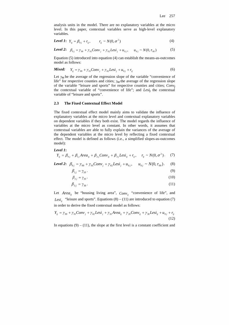
analysis units in the model. There are no explanatory variables at the micro level. In this paper, contextual variables serve as high-level explanatory variables.

Level 1: ,0 ijjij rY += β ) ,0(~ 2σNrij (4)

Level 2: ,00201000 jjjj uLesiConv +++= γγγβ ) ,0(~ 000 τNu j (5)

Equation (5) introduced into equation (4) can establish the means-as-outcomes model as follows:

Mixed: ijjjjij ruLesiConvY ++++= 0020100 γγγ (6)

Let γ01 be the average of the regression slope of the variable “convenience of life” for respective counties and cities; γ02 the average of the regression slope of the variable “leisure and sports” for respective counties and cities; Convj the contextual variable of “convenience of life”; and Lesij the contextual variable of “leisure and sports”. 2.3 The Fixed Contextual Effect Model The fixed contextual effect model mainly aims to validate the influence of explanatory variables at the micro level and contextual explanatory variables on dependent variables if they both exist. The model regards the influence of variables at the micro level as constant. In other words, it assumes that contextual variables are able to fully explain the variances of the average of the dependent variables at the micro level by reflecting a fixed contextual effect. The model is defined as follows (i.e., a simplified slopes-as-outcomes model):

Level 1: ,3210 ijijjijjijjjij rLesiConvAreaY ++++= ββββ ) ,0(~ 2σNrij

. (7)

Level 2: ,00201000 jjjj uLesiConv +++= γγγβ ) ,0(~ 000 τNu j . (8)

101 γβ j = . (9)

202 γβ j = . (10)

303 γβ j = . (11)

Let ijArea be “housing living area”, ijConv “convenience of life”, and

ijLesi “leisure and sports”. Equations (8) – (11) are introduced to equation (7)

in order to derive the fixed contextual model as follows:

ijjijijijjjij ruLesiConvAreaLesiConvY +++++++= 0302010020100 γγγγγγ

(12)

In equations (9) – (11), the slope at the first level is a constant coefficient and


there is no explanatory variable at the second level. The purpose is to eliminate cross-level interactions and random effects. If 01γ and 02γ are

significantly different from 0, contextual effects exist. At this point, jConv

or jLesi at the second macro level is known as the “contextual variable”.

2.4 The Random Contextual Effect Model The random contextual effect model considers the influence of the variables at the micro level on the dependent variables as randomness changes. It is possible that there are variances between groups. Therefore, contextual variables are able to explain the variances of the averages of dependent variables at the micro level. The portions that cannot be explained will be absorbed by the error terms. The model is defined as follows:


(13)

Level 2:

,00201000 jjjj uLesiConv +++= γγγβ ) ,0(~ 000 τNu j (14)

),0(~, 1111101 τ Nu uγβ jjj += . (15)

),0(~, 2222202 τ Nu uγβ jjj += . (16)

),0(~, 3333303 τ Nu uγβ jjj += . (17)

where u1j is the difference between the average regression slope of the “area” of the j-th county (city) and the average of the average regression slope of the “area” of respective counties and cities. The variance is τ11. u2j is the difference between the average regression slope of the “convenience of life” of the j-th county (city) and the average of the average regression slope of the “convenience of life” of respective counties and cities. The variance is τ22. u3j is the difference between the average regression slope of the “leisure and sports” of the j-th county (city) and the average of the average regression slope of the “leisure and sports” of respective counties and cities. The variance is τ33. The introduction of equations (14) – (17) into equation (13) leads to the derivation of the random contextual effect model as follows:

321

0302010020100

ijjjj

jijijijjjij

ruuu

uLesiConvAreaLesiConvY

++++

++++++= γγγγγγ (18)

2.5 The Moderate Contextual Effect Model The moderate contextual effect model considers the influence of the

Lee 259

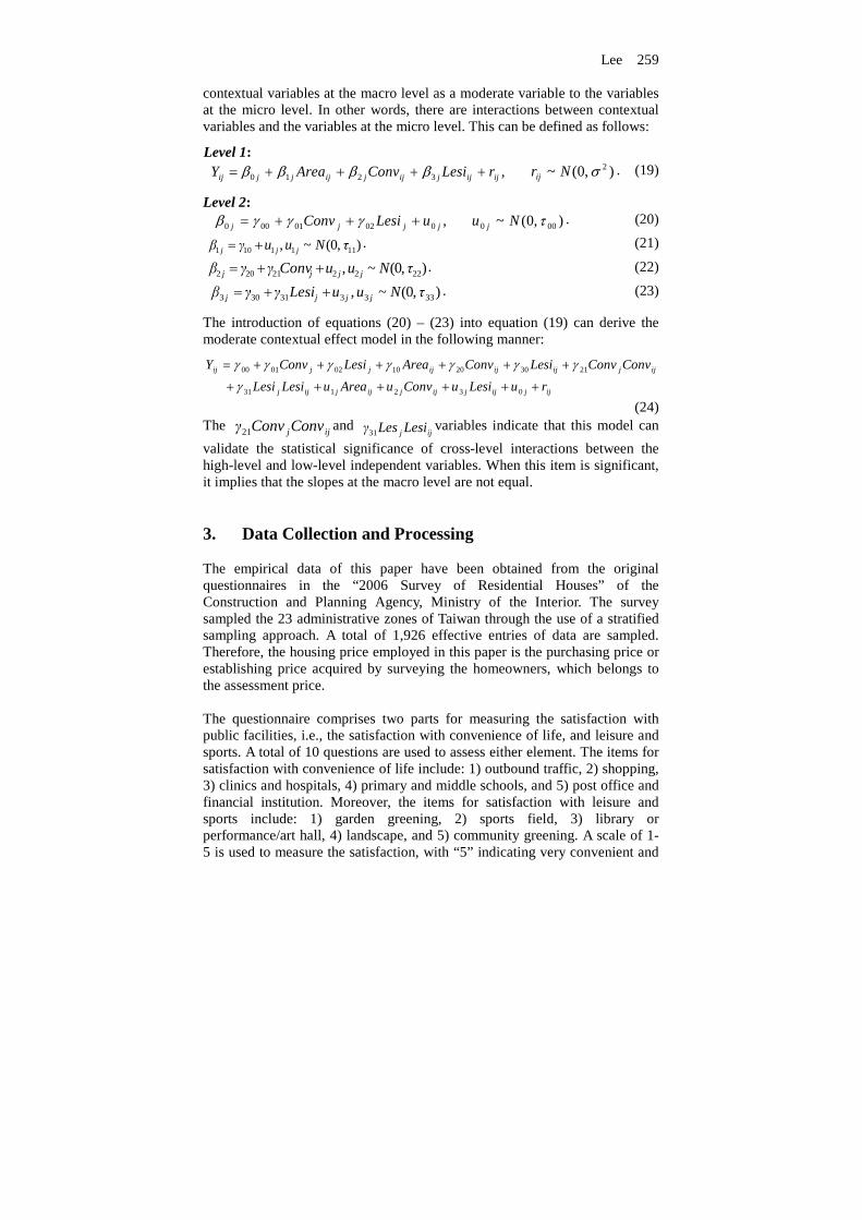
contextual variables at the macro level as a moderate variable to the variables at the micro level. In other words, there are interactions between contextual variables and the variables at the micro level. This can be defined as follows:


. (19)

Level 2: ,00201000 jjjj uLesiConv +++= γγγβ ) ,0(~ 000 τNu j

. (20)

),0(~, 1111101 τ Nu uγβ jjj += . (21)

),0(~, 222221202 τ Nu uConvγγβ jjjj ++= . (22)

),0(~, 333331303 τ Nu uLesiγγβ jjjj ++= . (23)

The introduction of equations (20) – (23) into equation (19) can derive the moderate contextual effect model in the following manner:

032131

21302010020100

ijjijjijjijjijj

ijjijijijjjij

ruLesiuConvuAreauLesiLesi

ConvConvLesiConvAreaLesiConvY

++++++

++++++=

γγγγγγγγ

(24) The ijjConvConvγ21 and

ijj LesiLesγ31variables indicate that this model can

validate the statistical significance of cross-level interactions between the high-level and low-level independent variables. When this item is significant, it implies that the slopes at the macro level are not equal. 3. Data Collection and Processing The empirical data of this paper have been obtained from the original questionnaires in the “2006 Survey of Residential Houses” of the Construction and Planning Agency, Ministry of the Interior. The survey sampled the 23 administrative zones of Taiwan through the use of a stratified sampling approach. A total of 1,926 effective entries of data are sampled. Therefore, the housing price employed in this paper is the purchasing price or establishing price acquired by surveying the homeowners, which belongs to the assessment price. The questionnaire comprises two parts for measuring the satisfaction with public facilities, i.e., the satisfaction with convenience of life, and leisure and sports. A total of 10 questions are used to assess either element. The items for satisfaction with convenience of life include: 1) outbound traffic, 2) shopping, 3) clinics and hospitals, 4) primary and middle schools, and 5) post office and financial institution. Moreover, the items for satisfaction with leisure and sports include: 1) garden greening, 2) sports field, 3) library or performance/art hall, 4) landscape, and 5) community greening. A scale of 1- 5 is used to measure the satisfaction, with “5” indicating very convenient and


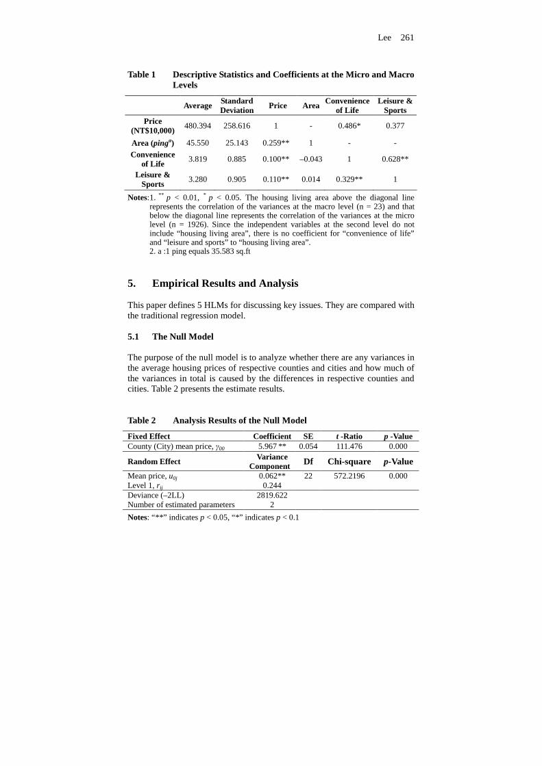
very satisfied, “4” indicating convenient and satisfied, “3” indicating OK and ordinary, “2” indicating not convenient and not satisfied, and “1” indicating very inconvenient and very unsatisfied. The satisfaction with regional public facilities includes satisfaction with convenience of life, and leisure and sports. As this paper cannot obtain the data required for high-level analytical variables, it adopts a composition approach (Kozlowski and Klein, 2000) by collating data that pertains to low-level individuals for analysis. This paper refers to housing prices as a dependent variable. Since the variables collated by this paper with regard to the regional public facilities (convenience of life and leisure and sports) are shared constructs, the data is collated from individual residents (Klein, Dansereau, and Hall, 1994). Therefore, prior to any cross-level analysis, it is necessary to examine the appropriateness of the aggregation of variables into collective levels. In other words, it is necessary to inspect the within-group agreement (James, Demaree, and Wolf, 1993) and between-group variation of the data (Hofmann, 1997; Klein and Kozlowski, 2000) prior to the aggregation of data at the micro level into a collective one. This paper uses rwgj as the validation indicator (James, Demaree, and Wolf, 1993) to verify the fitness of data aggregation (if rwgj > 0.70, it implies that the data is fit for aggregation). With regard to the validation of between-group variation, this paper uses ICC as the indicator. The calculation finds that the average convenience of life; rwgj, is 0.932 (between 0.847 and 0.983), the mode is 0.660, and ICC is 0.2027. These numbers illustrate the reasonability of aggregation procedures. 4. Description of Sample Statistics This paper runs SPSS 16.0 in order to process the variables at the micro and macro levels prior to the empirical analysis with HLM 6.02. Table 1 summarizes the description of statistics with regard to all variables. The average housing price of all 23 counties and cities is NT$480.394, with a standard deviation of NT$258.616. The average housing area of the 23 counties and cities is 45.55 pings, with a standard deviation of 25.143 pings. Table 1 presents the averages and standard deviations of the satisfaction with convenience of life, and leisure and sports. As far as the micro level is concerned, the coefficients of prices and housing living areas, convenience of life, and leisure and sports are 0.259, 0.100, and 0.110, respectively, and all attain the 1% significance level. In other words, housing living areas, convenience of life, leisure and sports are all positively correlated with housing prices. With regard to the macro level, the coefficients of prices, convenience of life, and leisure and sports are 0.486 and 0.377, respectively. The coefficients of prices and convenience of life attain the 5% significance level. In other words, convenience of life and housing prices are positively correlated.

Lee 261

Table 1 Descriptive Statistics and Coefficients at the Micro and Macro Levels

Average Standard Deviation Price Area Convenience

of Life Leisure &

Sports Price

(NT$10,000) 480.394 258.616 1 - 0.486* 0.377

Area (pinga) 45.550 25.143 0.259** 1 - -

Convenience of Life

3.819 0.885 0.100** –0.043 1 0.628**

Leisure & Sports

3.280 0.905 0.110** 0.014 0.329** 1

Notes: 1. ** p < 0.01, * p < 0.05. The housing living area above the diagonal line represents the correlation of the variances at the macro level (n = 23) and that below the diagonal line represents the correlation of the variances at the micro level (n = 1926). Since the independent variables at the second level do not include “housing living area”, there is no coefficient for “convenience of life” and “leisure and sports” to “housing living area”.

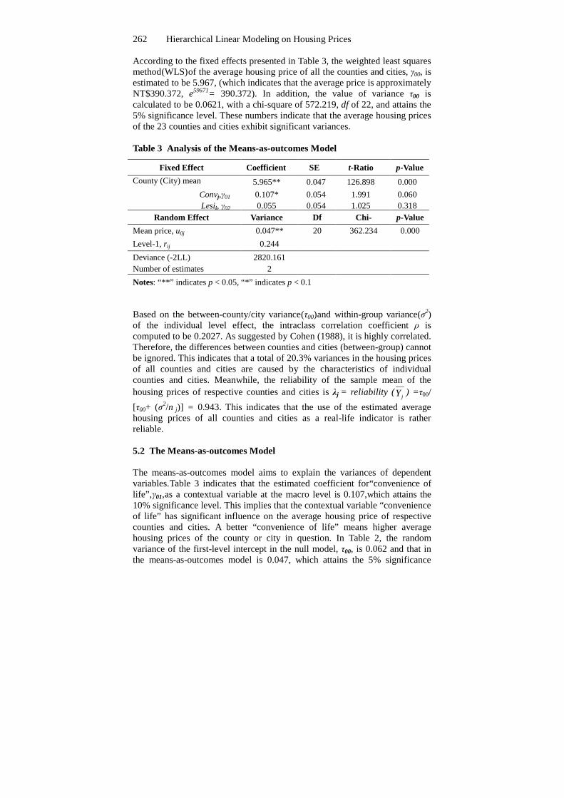
2. a :1 ping equals 35.583 sq.ft 5. Empirical Results and Analysis This paper defines 5 HLMs for discussing key issues. They are compared with the traditional regression model. 5.1 The Null Model The purpose of the null model is to analyze whether there are any variances in the average housing prices of respective counties and cities and how much of the variances in total is caused by the differences in respective counties and cities. Table 2 presents the estimate results. Table 2 Analysis Results of the Null Model

Fixed Effect Coefficient SE t -Ratio p -Value County (City) mean price, γ00 5.967 ** 0.054 111.476 0.000

Random Effect Variance Component Df Chi-square p-Value

Mean price, u0j 0.062** 22 572.2196 0.000 Level 1, rij 0.244 Deviance (–2LL) 2819.622 Number of estimated parameters 2

Notes: “**” indicates p < 0.05, “*” indicates p < 0.1


According to the fixed effects presented in Table 3, the weighted least squares method (WLS) of the average housing price of all the counties and cities, γ00, is estimated to be 5.967, (which indicates that the average price is approximately NT$390.372, e59671= 390.372). In addition, the value of variance τ00 is calculated to be 0.0621, with a chi-square of 572.219, df of 22, and attains the 5% significance level. These numbers indicate that the average housing prices of the 23 counties and cities exhibit significant variances. Table 3 Analysis of the Means-as-outcomes Model

Fixed Effect Coefficient SE t-Ratio p-Value

County (City) mean price,γ

5.965** 0.047 126.898 0.000

Convj,γ01 0.107* 0.054 1.991 0.060 Lesij, γ02 0.055 0.054 1.025 0.318

Random Effect Variance Df Chi- Square

p-Value

Mean price, u0j 0.047** 20 362.234 0.000

Level-1, rij 0.244

Deviance (-2LL) 2820.161 Number of estimates 2

Notes: “**” indicates p < 0.05, “*” indicates p < 0.1 Based on the between-county/city variance (τ00) and within-group variance (σ2) of the individual level effect, the intraclass correlation coefficient ρ is computed to be 0.2027. As suggested by Cohen (1988), it is highly correlated. Therefore, the differences between counties and cities (between-group) cannot be ignored. This indicates that a total of 20.3% variances in the housing prices of all counties and cities are caused by the characteristics of individual counties and cities. Meanwhile, the reliability of the sample mean of the housing prices of respective counties and cities is λj = reliability (

jY ) =τ00/

[τ00+ (σ2/n j)] = 0.943. This indicates that the use of the estimated average housing prices of all counties and cities as a real-life indicator is rather reliable. 5.2 The Means-as-outcomes Model The means-as-outcomes model aims to explain the variances of dependent variables. Table 3 indicates that the estimated coefficient for “convenience of life”, γ01, as a contextual variable at the macro level is 0.107, which attains the 10% significance level. This implies that the contextual variable “convenience of life” has significant influence on the average housing price of respective counties and cities. A better “convenience of life” means higher average housing prices of the county or city in question. In Table 2, the random variance of the first-level intercept in the null model, τ00, is 0.062 and that in the means-as-outcomes model is 0.047, which attains the 5% significance

Lee 263

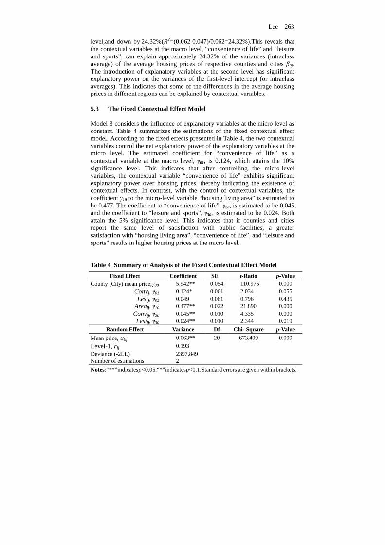
level, and down by 24.32% (R2= (0.062-0.047) /0.062=24.32%). This reveals that the contextual variables at the macro level, “convenience of life” and “leisure and sports”, can explain approximately 24.32% of the variances (intraclass average) of the average housing prices of respective counties and cities β0j. The introduction of explanatory variables at the second level has significant explanatory power on the variances of the first-level intercept (or intraclass averages). This indicates that some of the differences in the average housing prices in different regions can be explained by contextual variables. 5.3 The Fixed Contextual Effect Model Model 3 considers the influence of explanatory variables at the micro level as constant. Table 4 summarizes the estimations of the fixed contextual effect model. According to the fixed effects presented in Table 4, the two contextual variables control the net explanatory power of the explanatory variables at the micro level. The estimated coefficient for “convenience of life” as a contextual variable at the macro level, γ01, is 0.124, which attains the 10% significance level. This indicates that after controlling the micro-level variables, the contextual variable “convenience of life” exhibits significant explanatory power over housing prices, thereby indicating the existence of contextual effects. In contrast, with the control of contextual variables, the coefficient γ10 to the micro-level variable “housing living area” is estimated to be 0.477. The coefficient to “convenience of life”, γ20, is estimated to be 0.045, and the coefficient to “leisure and sports”,

γ30, is estimated to be 0.024. Both

attain the 5% significance level. This indicates that if counties and cities report the same level of satisfaction with public facilities, a greater satisfaction with “housing living area”, “convenience of life”, and “leisure and sports” results in higher housing prices at the micro level. Table 4 Summary of Analysis of the Fixed Contextual Effect Model

Fixed Effect Coefficient SE t-Ratio p-Value County (City) mean price,γ00 5.942** 0.054 110.975 0.000

Convj, γ01 0.124* 0.061 2.034 0.055 Lesij, γ02 0.049 0.061 0.796 0.435

Areaij, γ10 0.477** 0.022 21.890 0.000 Convij, γ20 0.045** 0.010 4.335 0.000 Lesiij, γ30 0.024** 0.010 2.344 0.019

Random Effect Variance Df Chi- Square p-Value

Mean price, u0j 0.063** 20 673.409 0.000

Level-1, rij 0.193 Deviance (-2LL) 2397.849 Number of estimations 2

Notes: “**” indicates p < 0.05. “*” indicates p < 0.1. Standard errors are given within brackets.


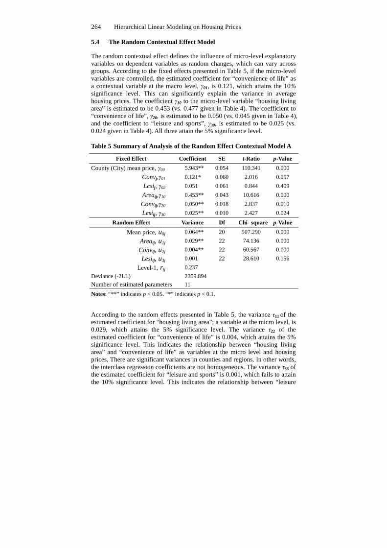
5.4 The Random Contextual Effect Model The random contextual effect defines the influence of micro-level explanatory variables on dependent variables as random changes, which can vary across groups. According to the fixed effects presented in Table 5, if the micro-level variables are controlled, the estimated coefficient for “convenience of life” as a contextual variable at the macro level, γ01,

is 0.121, which attains the 10% significance level. This can significantly explain the variance in average housing prices. The coefficient γ10 to the micro-level variable “housing living area” is estimated to be 0.453 (vs. 0.477 given in Table 4). The coefficient to “convenience of life”, γ20, is estimated to be 0.050 (vs. 0.045 given in Table 4), and the coefficient to “leisure and sports”, γ30, is estimated to be 0.025 (vs. 0.024 given in Table 4). All three attain the 5% significance level. Table 5 Summary of Analysis of the Random Effect Contextual Model A


County (City) mean price, γ00 5.943** 0.054 110.341 0.000

Convj,γ01 0.121* 0.060 2.016 0.057

Lesij, γ02 0.051 0.061 0.844 0.409

Areaij,γ10 0.453** 0.043 10.616 0.000

Convij,γ20 0.050** 0.018 2.837 0.010

Lesiij, γ30 0.025** 0.010 2.427 0.024

Random Effect Variance Df Chi- square p-Value

Mean price, u0j 0.064** 20 507.290 0.000

Areaij, u1j 0.029** 22 74.136 0.000

Convij, u2j 0.004** 22 60.567 0.000

Lesiij, u3j 0.001 22 28.610 0.156

Level-1, rij 0.237

Deviance (-2LL) 2359.894

Number of estimated parameters 11

Notes: “**” indicates p < 0.05. “*” indicates p < 0.1. According to the random effects presented in Table 5, the variance τ11 of the estimated coefficient for “housing living area”; a variable at the micro level, is 0.029, which attains the 5% significance level. The variance τ22

of the estimated coefficient for “convenience of life” is 0.004, which attains the 5% significance level. This indicates the relationship between “housing living area” and “convenience of life” as variables at the micro level and housing prices. There are significant variances in counties and regions. In other words, the interclass regression coefficients are not homogeneous. The variance τ33

of the estimated coefficient for “leisure and sports” is 0.001, which fails to attain the 10% significance level. This indicates the relationship between “leisure

Lee 265

and sports” as a micro-level variable with housing prices. There are no significant differences across counties and cities. Furthermore, this paper eliminates the random effects of the micro-level variable “leisure and sports” and presents the analysis results in Table 6. The random contextual effect model A is compared with the random contextual effect model B. In this comparison, the chi-square is 0.107 (2360.002 – 2359.894) and degrees of freedom at 4, which fail to attain the 5% significance level. Therefore, in the follow-up model analysis, this model fixes the micro-level variable “leisure and sports”, and does not consider the random effect of this variable. Table 6 Summary of Analysis of the Random Effect Contextual Model B


County (City) mean price,γ00 5.943** 0.054 110.444 0.000 Convj, γ01 0.121* 0.060 2.022 0.056 Lesij, γ02 0.051 0.061 0.842 0.410 Areaij, γ10 0.453** 0.043 10.647 0.000

Convij, γ20 0.051** 0.018 2.849 0.010 Lesiij, γ30 0.024** 0.010 2.331 0.020

Random Effect Variance Df Chi- square p-Value

Mean price, u0j 0.063** 20 523.746 0.000

Areaij, u1j 0.029** 22 74.939 0.000

Convij, u2j 0.004** 22 54.400 0.000

Level-1, rij 0.185 Deviance (-2LL) 2360.002 Number of estimated parameters 7

Notes: “**” indicates p < 0.05. “*” indicates p < 0.1. 5.5 The Moderate Contextual Effect Model The moderate contextual effect model regards the influence of contextual variables as the moderating variables at the micro level. According to the fixed effects listed in Table 7, the estimated coefficient γ10 for the micro-level contextual variable “housing living area”, “convenience of life”, γ20,

and “leisure and sports”, γ30, are 0.453, 0.051, and 0.024, respectively, which attain the 5% significance level. In other words, a higher satisfaction perceived by individual residents with convenience of life and leisure and sports result in a stronger influence on housing prices. The estimated coefficient for the second-level variable “convenience of life”, γ01, is 0.121, which attains the 10% significance level. This indicates the existence of contextual effects. The estimated coefficients of the interactions of contextual and micro-level variables, i.e., γ21 and γ31, fail to attain the 5% significance


level, thereby indicating that the explanatory power of micro-level variables is not subject to the moderation of contextual variables. According to the random effects presented in Table 7, the variance of the estimated coefficient for the micro-level variable “housing living area” τ11

is 0.032, which attains the 5% significance level. The variance of the estimated coefficient for the micro-level variable “convenience of life” τ22 is 0.004, which attains the 5% significance level. This indicates that the influence of the micro-level variable “convenience of life” on housing prices does not have identical within-group variances. Table 7 Summary of Analysis of the Moderate Contextual Effect Model

Fixed Effect Coefficient SE t -Ratio p-Value

County (City) mean price, β0j. Base, γ00 5.943** 0.054 110.444 0.000 Convj,γ01 0.121* 0.060 2.022 0.056 Lesij,γ02 0.051 0.060 0.842 0.410

β1j. Base ,γ10 0.453** 0.043 10.647 0.000 Convj,γ11 0.041 0.050 0.826 0.419 Lesij,γ12 - 0.014 0.073 -0.186 0.855

β2j. Base ,γ20 0.051** 0.018 2.849 0.010 Convj,γ21 - 0.029 0.017 -1.709 0.101

β3j. Base,γ30 0.024** 0.010 2.331 0.020 Lesij ,γ31 0.003 0.012 0.284 0.776

Random Effect Variance Df Chi-square p-Value

Mean price, u0j 0.064** 20 520.7332 0.000 Areaij, u1j 0.032** 20 73.4559 0.000 Convij, u2j 0.004** 21 48.7578 0.001

Level-1, rij 0.185 Deviance (-2LL) 2377.891 Number of estimated parameters 7

Notes: “**” indicates p < 0.05; “*” indicates p < 0. According to models 2 to 5, the variances in the explanatory power of macro-level (contextual variables) and micro-level explanatory variables are related to the determination of random effects. However, if the determination of random effects permits non-homogeneous interclass regression coefficients in the micro-level explanatory variables, the influence of contextual variables on the dependent variables at the micro level will be affected. For example, in the random contextual effect model, in addition to the variances in the averages of

Lee 267

dependent variables (intercept variances) across counties and cities, the explanatory powers of the two respective explanatory variables also exhibit intraclass variances (slope variances). This indicates that the HLM analysis is more flexible and accommodating in the tests of intraclass variances. 5.6 The Traditional Regression Analysis In order to verify the influence of micro-level and contextual variables, this paper uses 6 different multiple regression models to interpret the influence of explanatory variables. Furthermore, 23 counties and cities are studied; therefore, 22 dummy variables are generated. Among them, R1a and R1b contain the 3 micro-level variables, which make them low-level models. R2a and R2b contain 2 contextual variables, which make them high-level models. R3a and R3b contain both micro-level explanatory and contextual variables, which make them hybrid models. Among all the models, “a” indicates the multiple regression models that do not contain the dummy variables for counties and cities, whereas “b” indicates the models that contain the dummy variables for counties and cities. Table 8 summarizes the results of the analysis. Apparently, the explanatory variables at the micro level have better explanatory power over dependent variables. After the inclusion of the 22 dummy variables, the explanatory power of R1b regression model attains 0.619. In contrast, the variables at the macro level comprising contextual variables have weaker explanatory power over dependent variables. Even with the incorporation of dummy variables of counties and cities, the explanatory power of R2b regression model is only 0.469. The hybrid model comprises variables at both micro and macro levels; however, its explanatory power is maintained at 0.619. R3a and R3b both contain macro-level and contextual variables. Therefore, the interpretation of dependent variables by explanatory variables is the net influence with the effects on other independent variables under control. The coefficient β of contextual variables is the net effect with the micro-level variables under control. This is consistent with the contextual effects defined by Pedhazur (1997). According to Table 8, the parameter estimates of R3b and R1b indicate that the explanatory variables that are statistically significant at the micro level are completely identical. This indicates that the explanatory variables at the micro level are not subject to the influence of high-level contextual variables. However, the explanatory variables at the macro level fluctuate due to the influence of micro-level variables. R3b is the result after the incorporation of dummy variables. This paper compares R3a and R3b and finds that although the contextual variables in both models are statistically significant, the coefficient estimated for “convenience of life” in R3b has a negative value (- 0.354).


Another important aspect of model specification and testing is examining how closely the model fits the data. The deviance is a measure of the lack of fit between the data and the model. The deviance for any one model cannot be interpreted directly, but can be used to compare multiple models to one another. The difference of the deviances from each model is distributed as a chi-square statistic with degrees of freedom equal to the difference in the number of parameters estimated in each model. For example, consider Tables 7 and 8. The deviance for the moderate contextual effect model is 2377.891. The deviance for the traditional regression analysis is 2431.344. The difference between the two deviances is 53.453, which is compared to a chi-squared distribution with 5 df. The difference is significant, so there is evidence that the moderate contextual effect model (HLM) provides a better fit to the data than the traditional regression analysis (OLS). The above estimate indicates that it is possible to use 22 dummy variables to represent 23 counties and cities in the estimation of housing prices with a traditional regression model. The heterogeneous variance (non-random effect) of building characteristics must be considered. The model must define the interactions between the satisfaction of residents with public and regional public facilities. However, random effects are not taken into account from the perspective of the conventional linear model; the regression models omit an important explanatory variable. As a result, the estimated error variances are too high and the estimated standard error for the regression coefficient is too low. In other words, the test of the regression coefficient tends to reject the null hypothesis. This leads to an increase in the number of Type 1 errors. 6. Conclusions and Suggestions This paper adopts HLM in order to examine the influence of satisfaction with public facilities in close proximity and regional public facilities on housing prices. It also illustrates the characteristics and validation methods of “contextual effects”. Meanwhile, this paper analyzes the manner in which traditional regression methods and HLM process contextual variables in a multilevel data structure. This paper utilizes HLM, and its empirical study indicates the following: at the micro level, the influence of the variables “housing living area”, “convenience of life”, and “leisure and sports” on housing prices in respective counties and cities attains the 5% significance level. This indicates that the micro-level variables exhibit significant influence on housing prices in respective counties and cities. At the macro level, the predictability of the variable “convenience of life” on average housing prices of individual counties and cities attains the 5% significance level. It also explains approximately 24.32% of the variances for the average housing prices in respective counties and cities β0j. The influence of the satisfaction with

Lee 269

convenience of life in different counties and cities exhibits significant variances. In other words, the satisfaction with regional convenience of life boasts contextual effects, but not moderating effects, in terms of its influence on housing prices. Although the traditional regression analysis can answer the questions that pertain to the micro and macro levels, each analysis is only able to process one level. The explanatory power of low-level explanatory variables can be estimated with traditional regression analysis; however, the HLM contextual model is able to show more clearly how the low-level explanatory variables are influenced by contextual variables and how the results change4. Multilevel models provide a more appropriate analysis method for the products whose attributes are hierarchical. Therefore, a multilevel analysis can be advantageous when analyzing the residential housing market, which possesses a diverse and multilevel data structure.

4 Due to the influence of spatial heterogeneity, a traditional regression analysis is able to take into account building and regional characteristics, and defines the interactions between building and regional characteristics. However, the conventional statistical techniques are not able to fully explain the changes between building characteristics (micro-level variables) and housing prices due to regional differences (i.e., the contextual variables in this paper).

Lee Chung-Chang 270 2

70

Hierarch

ical Lin

ear Mo

de

ling

on

Ho

using

Prices

Table 8 Summary of Regression Analysis of Micro-Level and Macro-Level Variables as Factors Affecting Housing Prices

Low-level Model (R1) High-level Model (R2) Mixed-Model(R3)

Multi-regression

model (R1a) Dummy regression

model (R1b) Multi-regression


model (R2b) Multi-regression


model (R3b) B(SE) Beta t B(SE) Beta T B(SE) Beta t B(SE) Beta T B(SE) Beta t B(SE) Beta t

Constant 4.826 (0.092)

52.237** 4.527 (.080)

56.679** 5.989 (.013)

471.070** 6.174(.033)

184.485** 4.622(.089)

51.800** 4.524 (.081)

55.833**

Area .327 (.025)

.286 13.198** .480 (.022)

.419 21.963** .369(.024)

.322 15.485** .480 (.022)

.419 21.963**

Conv. of life

.070 (.012)

.126 5.813** .042 (.010)

.075 4.061** .038(.012)

.069 3.281** .042 (.010)

.075 4.061**

Micro

variable Leisure

& sports .041 (.012)

.074 3.410** .021 (.010)

.038 2.094* .020(.012)

.035 1.674 .021 (.010)

.038 2.094*

Conv. of life

.113

(.014)

.195 7.853** –.115

(.030)

–.199 –3.807** .128

(.014)

.220 9.225** –.205

(.027)

–.354 –7.507** Macro

variab

le

Leisure & sports

.082 (.016)

.126 5.060** .193(.031)

.293 6.261** .082(.016)

.125 5.262** .266 (.028)

.405 9.596**

△R2 .302 .192 .190

△F 24.417 55.429 39.536

Co

unty/C

ity (d

um

my) P

R2 .317 .619 .277 .469 .429 0.619

F 71.617 47.200 79.816 24.387 86.736 47.200

Total

P 0.000 0.000 0.000 0.000 0.000 0.000

* p < 0.05 ,** p < 0.01

Lee 271

References

Anselin, L. (1988). Spatial Econometrics: Methods and Models. Kluwer Academic Publishers: Netherlands Dordercht. Anselin, L. (1989). What is Special about Spatial Data? : Alternative Perspectives on Spatial Data Analysis. National Center for Geographic Information and Analysis: Santa Barbara. Basu, S., and Thibodeau, T. G. (1998). Analysis of Spatial Autocorrelation in House Prices, Journal of Real Estate Finance and Economics, 17, 1, 61-85. Bitter, C., Mulligan, G. F., and Dall’erba, S. (2007). Incorporating Spatial Variation in Housing Attribute Prices: A Comparison of Geographically Weighted Regression and the Spatial Expansion Method, Journal of Geographical Systems, 9, 1, 7-27. Bourassa, S. C., Hoesli, M. and Peng, V. S. (2003). Do Housing Submarkets Really Matter? Journal of Housing Economics, 12, 1, 12-28. Brown, K. H. and Uyar, B. (2004). A Hierarchical Linear Model Approach for Assessing the Effects of House and Neighborhood Characteristics on Housing Prices, Journal of Real Estate Practice and Education, 7, 1, 15-23. Case, K. E., and Mayer, C. J. (1996). Housing Price Dynamics within a Metropolitan Area, Regional Science and Urban Economics, 26, 3-4, 387-407. Chiou, H. and Wen, F. H. (2007). Hierarchical Linear Modeling of Contextual Effects: An Example of Organizational Climate of Creativity at Schools and Teacher’s Creativity Performance, Journal of Education ＆ Psychology, 30, 1, 1-35. Cohen, J. (1988). Statistical Power Analysis for the Behavioral Sciences, Lawrence Erlbaum Associates: Hilldale. Courgeau, D. (2003). Methodology and Epistemology of Multilevel Analysis: Approaches from Different Social Sciences, Kluwer Academic Publishers: Netherlands Dordercht. Fotheringham, S., Brunsdon, C., and Charlton, M. (1988). Geographically Weighted Regression: A Natural Evolution of the Expansion Method for Spatial Data Analysis, Environment and Planning, A, 30, 1905–1927.

272 Hierarchical Linear Modeling on Housing Prices Goodman, A. C. (1981). Housing Submarkets within Urban Areas: Definitions and Evidence, Journal of Regional Science, 21, 2, 175-185. Goodman, A. C. and Thibodeau, T. C. (1998). Housing Market Segmentation, Journal of Housing Economics, 7, 2, 121-143. Hofmann, D. A. (1997). An Overview of the Logic and Rationale of Hierarchical Linear Models, Journal of Management, 23, 723-744. James, L. R., Demaree, R. G. and Wolf, G. (1993). Rwg: An Assessment of Within-group Rater Agreement, Journal of Applied Psychology, 78, 306- 309.

Jones, K. and Bullen, N. (1994). Contextual Models of Urban House Prices: A Comparison of Fixed and Random Coefficient Models Developed by Expansion, Economic Geography, 70, 252-272. Klein, K. J., Dansereau, F. and Hall, R. J. (1994). Levels Issues in Theory Development, Data Collection, and Analysis, Academy of Management Journal, 19, 195-229. Kozlowski, S. W. J. and Klein, K. J. (2000). A Multilevel Approach to Theory and Research in Organization: Contextual, Temporal, and Emergent Processes, Multilevel Theory, Research, and Methods in Organization: Foundation, Extensions, and New Directions, Jossey Bass: San Francisco. Kreft, I. and de Leeuw, J. (1998). Introducing Multilevel Modeling. Sage Thousand Oaks: California. McGraw, K. O. and Wong, S. P. (1996). Forming Inferences about Some Intraclass Correlation Coefficients, Psychological Methods, 1, 1, 30-46. Pedhazur, E. (1997). Multiple Regression in Behavioral Research: Explanation and Prediction, FL: Holt, Rinehart, and Winston (3rd Ed.) Inc, Orlando. Raudenbush, S. W. and A. S. Bryk. Hierarchical Linear Models: Applications and Data Analysis Methods, Sage Publications Inc: Thousand Oaks. Snijders, T. A. B. and R. J. Bosker. (1999). Multilevel Analysis: An Introduction to Basic and Advanced Multilevel Modeling, Sage Publications Inc: London.

Hierarchical Linear Modeling to Explore the Influence of ...

Documents

Transcript of Hierarchical Linear Modeling to Explore the Influence of ...