Hierarchical Clustering of Hyperspectral Images

using Rank-Two Nonnegative Matrix Factorization

Nicolas Gillis⇤ Da Kuang† Haesun Park†

Abstract

In this paper, we design a hierarchical clustering algorithm for high-resolution hyperspectralimages. At the core of the algorithm, a new rank-two nonnegative matrix factorizations (NMF)algorithm is used to split the clusters, which is motivated by convex geometry concepts. Themethod starts with a single cluster containing all pixels, and, at each step, (i) selects a cluster insuch a way that the error at the next step is minimized, and (ii) splits the selected cluster into twodisjoint clusters using rank-two NMF in such a way that the clusters are well balanced and stable.The proposed method can also be used as an endmember extraction algorithm in the presence ofpure pixels. The e↵ectiveness of this approach is illustrated on several synthetic and real-worldhyperspectral images, and shown to outperform standard clustering techniques such as k-means,spherical k-means and standard NMF.

Keywords. nonnegative matrix factorization, rank-two approximation, convex geometry, high-resolution hyperspectral images, hierarchical clustering, endmember extraction algorithm.

1 Introduction

A hyperspectral image (HSI) is a set of images taken at many di↵erent wavelengths (usually between100 and 200), not just the usual three visible bands of light (red at 650nm, green at 550nm, and blue at450nm). An important problem in hyperspectral imaging is blind hyperspectral unmixing (blind HU):given a HSI, the goal is to recover the constitutive materials present in the image (the endmembers)and the corresponding abundance maps (that is, determine which pixel contains which endmemberand in which quantity). Blind HU has many applications such as quality control in the food industry,analysis of the composition of chemical compositions and reactions, monitoring the development andhealth of crops, monitoring polluting sources, military surveillance, and medical imaging; see, e.g., [8]and the references therein.

Let us associate a matrix M 2 Rm⇥n+ to a given HSI with m spectral bands and n pixels as follows:

the (i, j)th entry M(i, j) of matrix M is the reflectance of the jth pixel at the ith wavelength (thatis, the fraction of incident light that is reflected by the ith pixel at the jth wavelength). Hence eachcolumn of M is equal to the spectral signature of a pixel while each row is a vectorized image at agiven wavelength. The linear mixing model (LMM) assumes that the spectral signature of each pixelis a linear combination of the spectral signatures of the endmembers, where the weights in the linearcombination are the abundances of each endmember in that pixel. For example, if a pixel contains 40%of aluminum and 60% of copper, then its spectral signature will be 0.4 times the spectral signatureof the aluminum plus 0.6 times the spectral signature of the copper. This is a rather natural model:

⇤Department of Mathematics and Operational Research, Faculte Polytechnique, Universite de Mons, Rue de Houdain9, B-7000 Mons, Email: nicolas.gillis@umons.ac.be. This work was carried on when NG was a postdoctoral researcherof the fonds de la recherche scientifique (F.R.S.-FNRS).

†School of Computational Science and Engineering, Georgia Institute of Technology, Atlanta, GA 30332-0765, USA.Emails: {da.kuang,hpark}@cc.gatech.edu. The work of these authors was supported in part by the National ScienceFoundation (NSF) grants CCF-0808863 and CCF-0732318.

1

arX

iv:1

310.

7441

v4 [

cs.C

V]

19 A

ug 2

014

we assume that 40% of the light is reflected by the aluminum while 60% is by the copper, whilenon-linear e↵ects are neglected (such as the light interacting with multiple materials before reflectingo↵, or atmospheric distortions).

Assuming the image contains r endmembers, and denoting W (:, k) 2 Rm (1 k r) the spectralsignatures of the endmembers, the LMM can be written as

M(:, j) =rX

k=1

W (:, k)H(k, j) 1 j n,

where H(k, j) is the abundance of the kth endmember in the jth pixel, hencePr

k=1H(k, j) = 1 forall j, which is referred to as the abundance sum-to-one constraint. Under the LMM and given aHSI M , blind HU amounts to recovering the spectral signatures of the endmembers (matrix W ) alongwith the abundances (matrix H). Since all matrices involved M , W and H are nonnegative, blind HUunder the LMM is equivalent to nonnegative matrix factorization (NMF): Given a nonnegative matrixM 2 Rm⇥n

+ and a factorization rank r, find two nonnegative matrices W 2 Rm⇥r+ and H 2 Rr⇥n

+

such that M ⇡ WH. Unfortunately, NMF is NP-hard [35] and highly ill-posed [16]. Therefore,in practice, it is crucial to use the structure of the problem at hand to develop e�cient numericalschemes for blind HU. This is usually achieved using additional constraints or regularization termsin the objective function, e.g., the sum-to-one constraint on the columns of H (see above), sparsityof the abundance matrix H (most pixels contain only a few endmembers), piecewise smoothness ofthe spectral signatures W (:, k) [24], and spatial information [38] (that is, neighboring pixels are morelikely to contain the same materials). Although these priors make the corresponding NMF problemsmore well-posed, the underlying optimization problems to be solved are still computationally di�cult(and only local minimum are usually obtained). We refer the reader to the survey [8] for more detailsabout blind HU.

In this paper, we make an additional assumption, namely that most pixels are dominated mostlyby one endmember, and our goal is to cluster the pixels accordingly. In fact, clustering the pixels ofa HSI only makes sense for relatively high resolution images. For such images, it is often assumedthat, for each endmember, there exists at least one pixel containing only that endmember, that is, forall 1 k r there exists j such that M(:, j) = W (:, k). This is the so-called pure-pixel assumption.The pure-pixel assumption is equivalent to the separability assumption (see [21] and the referencestherein) which makes the corresponding NMF problem tractable, even in the presence of noise [5].Hence, blind HU can be solved e�ciently under the pure-pixel assumption. Mathematically, a matrixM 2 Rm⇥n is r-separable if it can be written as

M = WH = W [Ir, H0]⇧,

where W 2 Rm⇥r, H 0 � 0 and ⇧ is a permutation matrix. If M is a HSI, we have, as before, that

⇧ The number r is the number of endmembers present in the HSI.

⇧ Each column of W is the spectral signature of an endmember.

⇧ Each column of H is the abundance vector of a pixel. More precisely, the entry H(i, j) is theabundance of the ith endmember in the jth pixel.

Because the column of H sum to one, each column of M belongs to the convex hull of the columnsof W , that is, conv(M) ✓ conv(W ). The pure-pixel assumption requires that conv(M) = conv(W ),that is, that the vertices of the convex hull of the columns of M are the columns of W ; see the topof Figure 1 for an illustration in the rank-three case. Hence, the separable NMF problem (or, equiva-lently, blind HU under the LMM and the pure-pixel assumption) reduces to identifying the vertices ofthe convex hull of the columns of M . However, in noisy settings, this problem becomes more di�cult,

2

and although some robust algorithms have been proposed recently (see, e.g., [17] and the referencestherein), they are typically rather sensitive to noise and outliers.

Motivated by the fact that in high-resolution HSI’s, most pixels are mostly dominated by oneendmember, we develop in this paper a practical and theoretically well-founded hierarchical clusteringtechnique. Hierarchical clustering based on NMF has been shown to be faster than flat clustering andcan often achieve similar or even better clustering quality [28]. At the core of the algorithm is theuse of rank-two NMF that splits a cluster into two disjoint clusters. We study the unique property ofrank-two NMF as opposed to a higher-rank NMF. We also propose an e�cient algorithm for rank-twoNMF so that the overall problem of hierarchical clustering of HSI’s can be e�ciently solved.

The paper is organized as follows. In Section 2, we describe our hierarchical clustering approach(see Algorithm 1 referred to as H2NMF). At each step, a cluster is selected (Section 2.1) and then splitinto two disjoint clusters (Section 2.2). The splitting procedure has a rank-two NMF algorithm at itscore which is described in Section 2.3 where we also provide some su�cient conditions under which theproposed algorithm recovers an optimal solution. In Section 2.4, we analyze the geometric propertiesof the hierarchical clustering. In Section 3, we show that it outperforms k-means, spherical k-means(either if they are used in a hierarchical manner, or directly on the full image) and standard NMFon synthetic and real-world HSI’s, being more robust to noise, outliers and absence of pure pixels.We also show that it can be used as an endmember extraction algorithms and outperforms vertexcomponent analysis (VCA) [31] and the successive projection algorithm (SPA) [3], two standard andwidely used techniques.

2 Hierarchical Clustering for HSI’s using Rank-Two NMF

As mentioned in the introduction, for high-resolution HSI, one can assume that most pixels containmostly one material. Hence, given a high-resolution HSI with r endmembers, it makes sense tocluster the pixels into r clusters, each cluster corresponding to one endmember. Mathematically,given the HSI M 2 Rm⇥n

+ , we want to find r disjoint clusters Kk ⇢ {1, 2, . . . n} for 1 k r so that[k=1,2,...,rKk = {1, 2, . . . n} and so that all pixels in Kk are dominated by the same endmember.

In this paper, we assume the number of endmembers is known in advance. In fact, the problemof determining the number of endmembers (also known as model order selection) is nontrivial andout of the scope of this paper; see, e.g., [7]. However, a crucial advantage of our approach is thatit decomposes the data hierarchically and hence provides the user with a hierarchy of materials (see,e.g., Figures 7 and 14). In particular, the algorithm does not need to be rerun from scratch if thenumber of clusters required by the user is modified.

In this section, we propose an algorithm to cluster the pixels of a HSI in a hierarchical manner.More precisely, at each step, given the current set of clusters {Kk}pk=1, we select one of the clusters andsplit it into two disjoint clusters. Hierarchical clustering is a standard technique in data mining thatorganizes a data set into a tree structure of items. It is widely used in text analysis for e�cient browsingand retrieval [37, 28, 9], as well as exploratory genomic study for grouping genes participating in thesame pathway [12]. Another example is to segment an image into a hierarchy of regions according todi↵erent cues in computer vision such as contours and textures [4]. In contrast to image segmentationproblems, our focus is to obtain a hierarchy of materials from HSI’s taken at hundreds of wavelengthsinstead of the three visible wavelengths.

At each step of a hierarchical clustering technique, one has to address the following two questions:

1. Which cluster should be split next?

2. How do we split the selected cluster?

3

These two building blocks for our hierarchical clustering technique for HSI’s are described in thefollowing sections.

2.1 Selecting the Leaf Node to Split

Eventually, we want to cluster the pixels into r disjoint clusters {Kk}rk=1, each corresponding to adi↵erent endmember. Therefore, each submatrix M(:,Kk) should be close to a rank-one matrix sincefor all j 2 Kk, we should have M(:, j) ⇡W (:, k), possibly up to a scaling factor (e.g., due to di↵erentillumination conditions in the image), where W (:, k) is the spectral signature of the endmember corre-sponding to the cluster Kk. In particular, in ideal conditions, that is, each pixel contains exactly onematerial and no noise is present, M(:,Kk) is a rank-one matrix. Based on this observation, we definethe error Ek corresponding to each cluster as follows

Ek = minX,rank(X)=1

||M(:,Kk)�X||2F = ||M(:,Kk)||2F � �21(M(:,Kk)).

We also define the total error E =Pr

k=1Ek. If we decide to split the kth cluster Kk into K1k and K2

k,the error corresponding to the columns in Kk is given by�||M(:,K1

k)||2F � �21(M(:,K1

k))�+�||M(:,K2

k)||2F � �21(M(:,K2

k))�

=�||M(:,K1

k)||2F + ||M(:,K2k)||2F )

�� ��21(M(:,K1

k)) + �21(M(:,K2

k))�

= ||M(:,Kk)||2F ���21(M(:,K1

k)) + �21(M(:,K2

k))�.

(Note that the error corresponding to the other clusters is unchanged.) Hence, if the kth cluster issplit, the total error E will be reduced by �2

1(M(:,K1k)) + �2

1(M(:,K2k)� �2

1(M(:,Kk)). Therefore, wepropose to split the cluster k for which �2

1(M(:,K1k))+�2

1(M(:,K2k)��2

1(M(:,Kk)) is maximized: thisleads to the largest possible decrease in the total error E at each step.

2.2 Splitting a Leaf Node

For the splitting procedure, we propose to use rank-two NMF. Given a nonnegative matrix M 2 Rm⇥n+ ,

rank-two NMF looks for two nonnegative matrices W 2 Rm⇥2+ and H 2 R2⇥n

+ such that WH ⇡ M .The motivation for this choice is two-fold:

⇧ NMF corresponds to the linear mixing model for HSI’s (see Introduction), and

⇧ Rank-two NMF can be solved e�ciently, avoiding the use of an iterative procedure as in standardNMF algorithms. In Section 2.3, we propose a new rank-two NMF algorithm using convexgeometry concepts from HSI; see Algorithm 4.

Suppose for now we are given a rank-two NMF (W,H) of M . Such a factorization is a two-dimensionalrepresentation of the data; more precisely, it projects the columns ofM onto a two-dimensional pointedcone generated by the columns ofW . Hence, a naive strategy to cluster the columns ofM is to choosingthe clusters as follows

C1 = { i | H(1, i) � H(2, i) } and C2 = { i | H(1, i) < H(2, i) }.Defining the vector x 2 [0, 1]n as

x(i) =H(1, i)

H(1, i) +H(2, i)for 1 i n,

the above clustering assignment is equivalent to taking

C1 = { i | xi � � } and C2 = { i | xi < � }, (2.1)

4

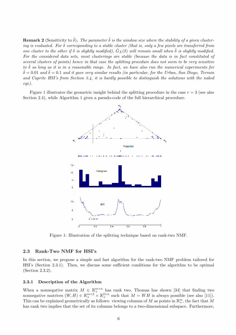
with � = 0.5. However, the choice of � = 0.5 is by no means optimal, and often leads to a rather poorseparation. In particular, if an endmember is located exactly between the two extracted endmembers,the corresponding cluster is likely to be divided into two which is not desirable (see Figure 1). Inthis section, we present a simple way to tune the threshold � 2 [0, 1] in order to obtain, in general,significantly better clusters C1 and C2.

Let us define the empirical cumulative distribution of x as follows

FX(�) =1

n

��{ i | xi � }�� 2 [0, 1], for � 2 [0, 1].

By construction, FX(0) = 0 and FX(1) = 1. Let us also define

GX(�) =1

n(� � �)

��{ i | � = max(0, � � �) xi min(1, � + �) = � }�� 2 [0, 1],

for � 2 [0, 1], and � 2 (0, 0.5) is a small parameter. The function GX(�) accounts for the number ofpoints in a small interval around �. Note that, assuming uniform distribution in the interval [0, 1], theexpected value of GX(�) is equal to one. In fact, since the entries of x are in the interval [0, 1], theexpected number of data points in an interval of length L is nL. In this work, we use � = 0.05.

Given �, we obtain two clusters C1 and C2; see Equation (2.1). We propose to choose a value of �such that

1. The clusters are balanced, that is, the two clusters contain, if possible, roughly the same numberof elements. Mathematically, we would like that FX(�) ⇡ 0.5.

2. The clustering is stable, that is, if the value of � is slightly modified, then only a few points aretransfered from one cluster to the other. Mathematically, we would like that GX(�) ⇡ 0.

We propose to balance these two goals by choosing � that minimizes the following criterion:

g(�) = � log⇣FX(�)

⇣1� FX(�)

⌘⌘

| {z }balanced clusters

+exp⇣GX(�)

⌘

| {z }stable clusters

. (2.2)

The first term avoids skewed classes, while the second promotes a stable clustering. Note that thetwo terms are somewhat well-balanced since, for FX(�) 2 [0.1, 0.9],

� log⇣FX(�)

⇣1� FX(�)

⌘⌘ 2.5,

and the expected value of GX(�) is one (see above). Note that depending on the application at hand,the two terms of g(�) can be balanced in di↵erent ways; for example, if one wants to allow very smallclusters to be extracted, then the first term of g(�) should be given less importance.

Remark 1 (Sensitivity to �). The splitting procedure is clearly very sensitive to the choice of �. Forexample, as described above, choosing � = 0.5 can give very poor results. However, if the functiong(�) is chosen in a sensible way, then the corresponding splitting procedure generates in general goodclusters. For example, we had first run all the experiments from Section 3 selecting � minimizing thefunction

g(�) = 4⇣FX(�)� 0.5

⌘2+⇣GX(�)

⌘2,

and it gave very similar results (sometimes slightly better, sometimes slightly worse). The advantageof the function (2.2) is that it makes sure no empty cluster is generated (since it goes to infinity whenFX(�) goes to 0 or 1).

5

Remark 2 (Sensitivity to �). The parameter � is the window size where the stability of a given cluster-ing is evaluated. For � corresponding to a stable cluster (that is, only a few pixels are transferred fromone cluster to the other if � is slightly modified), GX(�) will remain small when � is slightly modified.For the considered data sets, most clusterings are stable (because the data is in fact constituted ofseveral clusters of points) hence in that case the splitting procedure does not seem to be very sensitiveto � as long as it is in a reasonable range. In fact, we have also run the numerical experiments for� = 0.01 and � = 0.1 and it gave very similar results (in particular, for the Urban, San Diego, Terrainand Cuprite HSI’s from Section 3.4, it is hardly possible to distinguish the solutions with the nakedeye).

Figure 1 illustrates the geometric insight behind the splitting procedure in the case r = 3 (see alsoSection 2.4), while Algorithm 1 gives a pseudo-code of the full hierarchical procedure.

Figure 1: Illustration of the splitting technique based on rank-two NMF.

2.3 Rank-Two NMF for HSI’s

In this section, we propose a simple and fast algorithm for the rank-two NMF problem tailored forHSI’s (Section 2.3.1). Then, we discuss some su�cient conditions for the algorithm to be optimal(Section 2.3.2).

2.3.1 Description of the Algorithm

When a nonnegative matrix M 2 Rm⇥n+ has rank two, Thomas has shown [34] that finding two

nonnegative matrices (W,H) 2 Rm⇥2+ ⇥ R2⇥n

+ such that M = WH is always possible (see also [11]).This can be explained geometrically as follows: viewing columns of M as points in Rm

+ , the fact that Mhas rank two implies that the set of its columns belongs to a two-dimensional subspace. Furthermore,

6

Algorithm 1 Hierachical Clustering of a HSI based on Rank-Two NMF (H2NMF)

Input: A HSI M 2 Rm⇥n+ and the number r of clusters to generate.

Output: Set of disjoint clusters Ki for 1 i r with [iKi = {1, 2, . . . , n}.1: % Initialization2: K1 = {1, 2, . . . , n} and Ki = ; for 2 i r.3:�K1

1,K21

�= splitting(M,K1). % See Algorithm 2 and Section 2.2

4: K1i = K2

i = ; for 2 i r.5: for k = 2 : r do6: % Select the cluster to split; see Section 2.17: Let j = argmaxi=1,2,...r �

21(M(:,K1

i )) + �21(M(:,K2

i )� �21(M(:,Ki)).

8: % Update the clustering9: Kj = K1

j and Kk = K2j .

10: % Split the new clusters (Algorithm 2)

11:

⇣K1

j ,K2j

⌘= splitting(M,Kj) and

�K1k,K2

k

�= splitting(M,Kk).

12: end for

Algorithm 2 Splitting of a HSI using Rank-Two NMF

Input: A HSI M 2 Rm⇥n+ and a subset K ✓ {1, 2, . . . , n}.

Output: Set of two disjoint clusters K1 and K2 with K1 [K2 = K.

1: Let (W,H) be the rank-two NMF of M(:,K) computed by Algorithm 4.

2: Let x(i) = H(1,i)H(1,i)+H(2,i) for 1 i |K|.

3: Compute �⇤ as the minimum of g(�) defined in (2.2).4: K1 = { K(i) | x(i) � �⇤ } and K2 = { K(i) | x(i) < �⇤ }.

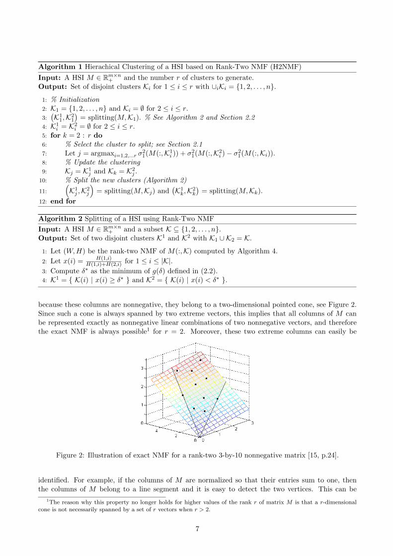
because these columns are nonnegative, they belong to a two-dimensional pointed cone, see Figure 2.Since such a cone is always spanned by two extreme vectors, this implies that all columns of M canbe represented exactly as nonnegative linear combinations of two nonnegative vectors, and thereforethe exact NMF is always possible1 for r = 2. Moreover, these two extreme columns can easily be

Figure 2: Illustration of exact NMF for a rank-two 3-by-10 nonnegative matrix [15, p.24].

identified. For example, if the columns of M are normalized so that their entries sum to one, thenthe columns of M belong to a line segment and it is easy to detect the two vertices. This can be

1The reason why this property no longer holds for higher values of the rank r of matrix M is that a r-dimensionalcone is not necessarily spanned by a set of r vectors when r > 2.

7

done for example using any endmember extraction algorithm under the linear mixing model and thepure-pixel assumption since they aim to detect the vertices (corresponding to the endmembers) ofa convex hull of a set of points (see Introduction). In this paper, we use the successive projectionalgorithm (SPA) [3] which is a highly e�cient and widely used algorithm; see Algorithm 3. Moreover,

Algorithm 3 Successive Projection Algorithm (SPA) [3, 21]

Input: Separable matrix M = W [Ir, H 0]⇧ where H 0 � 0, the sum of the entries of each column of H 0

is smaller than one, W is full rank and ⇧ is a permutation, and the number r of columns to beextracted.

Output: Set of indices K such that M(:,K) = W (up to permutation).

1: Let R = M , K = {}.2: for i = 1 : r do3: k = argmaxj ||R:j ||2.4: R

⇣I � R:kR

T:k

||R:k||22

⌘R.

5: K = K [ {k}.6: end for

it has been shown to be robust to any small perturbation of the input matrix [21]. Note that SPA isclosely related to the automatic target generation process algorithm (ATGP) [33] and the successivevolume maximization algorithm (SVMAX) [10]; see [30] for a survey about these methods. Note thatit would be possible to use more sophisticated endmember extraction algorithms for this step, e.g.,RAVMAX [1] or WAVMAX [10] which are more robust variants of SPA (although computationallymuch more expensive).

We can now describe our proposed rank-two NMF algorithm for HSI: It first projects the columnsof M into a two-dimensional linear space using the SVD (note that if the rank of input matrix is two,this projection step is exact), then identifies two important columns with SPA and projects them ontothe nonnegative orthant, and finally computes the optimal weights solving a nonnegative least squaresproblem (NNLS); see Algorithm 4.

Algorithm 4 Rank-Two NMF for HSI’s

Input: A nonnegative matrix M 2 Rm⇥n+ .

Output: A rank-two NMF (W,H) 2 Rm⇥2+ ⇥ R2⇥n

+ .1: % Compute an optimal rank-two approximation of M2: [U, S, V T ] = svds(M, 2); % See the Matlab function svds

3: Let X = SV (= UTUSV = UTM);4: % Extract two indices using SPA5: K = SPA(X, 2); % See Algorithm 36: W = max

�0, USV (:,K)

�;

7: H = argminY�0 ||M �WY ||2F ; % See Algorithm 5

Let us analyze the computational cost of Algorithm 4. The computation of the rank-two SVD ofM is O(mn) operations [22]. (Note that this operation scales well for sparse matrices as there existSVD methods that can handle large sparse matrices, e.g., the svds function of Matlab.) For HSI’s,m is much smaller than n (usually m ⇠ 200 while n ⇠ 106) hence it is faster to computing the SVDof M using the SVD of MMT which requires 2mn+ O(m2) operations; see, e.g., [31]. Note howeverthat this is numerically less stable as the condition number of the corresponding problem is squared.Extracting the two indices in step 5 with SPA requires O(n) operations [21], while computing theoptimal H requires solving n linear systems in two variables for a total computational cost of O(mn)

8

Algorithm 5 Nonnegative Least Squares with Two Variables [28]

Input: A matrix A 2 Rm⇥2 and a vector b 2 Rm.Output: A solution x 2 R2

+ to minx�0 ||Ax� b||2.1: % Compute the solution of the unconstrained least squares problem2: x = argminx ||Ax� b||2 (e.g., solve the normal equations (ATA)x = AT b).3: if x � 0 then4: return.5: else6: % Compute the solutions for x(1) = 0 and x(2) = 0 (the two possible active sets)

7: Let y =⇣0,max

⇣0, A(:,1)T b

||A(:,1)||22

⌘⌘and z =

⇣max

⇣0, A(:,2)T b

||A(:,2)||22

⌘, 0⌘.

8: if ||Ay � b||2 < ||Az � b||2 then9: x = y.

10: else11: x = z.12: end if13: end if

operations [28]. In fact, the NNLSmin

X2R2⇥n+

||M �WX||2F

where W 2 Rm⇥2+ can be decoupled into n independent NNLS in two variables since

||M �WX||2F =nX

i=1

||M(:, i)�WX(:, i)||22.

Algorithm 5 implements the algorithm in [28] to solve these subproblems.Finally, Algorithm 4 requires O(mn) operations which implies that the global hierarchical cluster-

ing procedure (Algorithm 1) requires at most O(mnr) operations. Note that this is rather e�cientand developing a significantly faster method would be di�cult. In fact, it already requires O(mnr)operations to compute the product of W 2 Rm⇥r and H 2 Rr⇥n, or to assign optimally n data pointsin dimension m to r cluster centroids using the Euclidean distance. Note however that in an idealcase, if the largest cluster is always divided into two clusters containing the same number of pixels(hence we would have a perfectly balanced tree), the number of operations reduces to O(mn log(r)).Hence, in practice, if the clusters are well balanced, the computational cost is rather in O(mn log(r))operations.

2.3.2 Theoretical Motivations

An mentioned above, rank-two NMF can be solved exactly for rank-two input matrices. Let us showthat Algorithm 4 does.

Theorem 1. If M is a rank-two nonnegative matrix whose entries of each column sum to one, thenAlgorithm 4 computes an optimal rank-two NMF of M .

Proof. Since M has rank-two and is nonnegative, there exists an exact rank-two NMF (F,G) ofM = FG = F (:, 1)G(1, :) +X(:, 2)Y (2, :) [34]. Moreover, since the entries of each column of M sumto one, we can assume without loss of generality that the entries of the each column of F and G sumto one as well. In fact, we can normalize the two columns of F so that their entries sum to one while

9

scaling the rows of G accordingly:

M =F (:, 1)

||F (:, 1)||1| {z }F 0(:,1)

||F (:, 1)||1G(1, :)| {z }G0(1,:)

+F (:, 2)

||F (:, 2)||1| {z }F 0(:,2)

||F (:, 2)||1G(2, :)| {z }G0(2,:)

= F 0G0.

Since the entries of each column of M and F 0 sum to one and M = F 0G0, the entries of each column ofG0 have to sum to one as well. Hence, the columns of M belong to the line segment [F 0(:, 1), F 0(:, 2)].

Let (U, S, V T ) be the rank-two SVD of M computed at step 2 of Algorithm 4, we have SV =UTM = (UTF 0)G0. Hence, the columns of SV belong to the line segment [UTF 0(:, 1),UTF 0(:, 2)] sothat SPA applied on SV will identify two indices corresponding to two columns of M being the verticesof the line segment defined by its columns [21, Th.1]. Therefore, any column ofM can be reconstructedwith a convex combination of these two extracted columns and Algorithm 4 will generate an exactrank-two NMF of M .

Corollary 1. Let M be a noiseless HSI with two endmembers satisfying the linear mixing model andthe sum-to-one constraint, then Algorithm 4 computes an optimal rank-two NMF of M .

Proof. By definition, M = WH where the columns of W are equal to the spectral signatures of thetwo endmembers and the columns of H are nonnegative and sum to one (see Introduction). Therest of the proof follows from the second part of the proof of Theorem 1. (Note that the pure-pixelassumption is not necessary.)

In practice, the sum-to-one constraints assumption is sometimes relaxed to the following: the sumof the entries of each column of H is at most one. This has several advantages such as allowing theimage to containing ‘background’ pixels with zero spectral signatures, or taking into account di↵erentintensities of light among the pixels in the image; see, e.g., [8]. In that case, Algorithm 4 works underthe additional pure-pixel assumption:

Corollary 2. Let M be a noiseless HSI with di↵erent illumination conditions, with two endmembers,and satisfying the linear mixing model and the pure-pixel assumption, then Algorithm 4 computes anoptimal rank-two NMF of M .

Proof. By assumption, M = W [I2, H 0]⇧ where H 0 is nonnegative and the entries of each column sumto at most one, and ⇧ is a permutation. This implies that the columns of M are now in the trianglewhose vertices are W (:, 1), W (:, 2) and the origin. Following the proof of Theorem 1, after the SVD,the columns of SV are in the triangle whose vertices are UTW (:, 1), UTW (:, 2) and the origin. HenceSPA will identify correctly the indices corresponding to W (:, 1) and W (:, 2) [21, Th.1] so that anycolumn of M can be reconstructed using these two columns.

At the first steps of the hierarchical procedure, rank-two NMF maps the data points into a two-dimensional subspace. However, the input matrix does not have rank-two if it contains more than twoendmembers. In the following, we derive some simple su�cient conditions to support the fact that therank-two SVD of a nonnegative matrix is nonnegative (or at least has most of its entries nonnegative).Let us refer to an optimal rank-two approximation of a matrix M as an optimal solution of

minA2Rm⇥n

||M �A||2F such that rank(A) = 2.

We will also refer to rank-two NMF as the following optimization problem

minU2Rm⇥2,V 2R2⇥n

||M � UV ||2F such that U � 0 and V � 0.

10

Lemma 1. Let M 2 Rm⇥n+ , A 2 Rm⇥n be an optimal rank-two approximation of M , and R = M �A

be the residual error. IfL = min

i,j(Mij) � max

i,jRij ,

then every entry of A is nonnegative.

Proof. If Akl < 0 for some (k, l), then L Mkl < Mkl �Akl = Rkl maxij Rij , a contradiction.

Corollary 3. Let M 2 Rm⇥n+ satisfy

L = mini,j

(Mij) � �3(M).

Then any optimal rank-two approximation of M is nonnegative.

Proof. This follows from Lemma 1 since, for any optimal rank-two approximation A of M with R =M �A, we have maxij Rij ||R||2 = �3(M).

Corollary 3 shows that a positive matrix close to having rank two and/or only containing relativelylarge entries is likely to have an optimal rank-two approximation which is nonnegative. Note thatHSI’s usually have mostly positive entries and, in fact, we have observed that the best rank-twoapproximation of real-world HSI’s typically contains mostly nonnegative entries (e.g., for the UrbanHSI more than 99.5%, for the San Diego HSI more than 99.9%, for the Cuprite HSI more than 99.98%,and for the Terrain HSI more than 99.8%; see Section 3.4 for a description of these data sets). Itwould be interesting to investigate further su�cient and necessary conditions for the optimal rank-two approximations of a nonnegative matrix to be nonnegative; this is a topic for further research.Note also Theorem 1 only holds for rank-two NMF and cannot be extended to more general caseswith an arbitrary r. Consequently, we designed Algorithm 4 specifically for rank-two NMF. However,Algorithm 4 is important in the context of hierarchical clustering where rank-two NMF is the corecomputation. We will show in Section 3 that our overall method achieves high e�ciency comparedto other hyperspectral unmixing methods. Moreover, if we flatten the obtained tree structure andlook at the clusters corresponding to the leaf nodes, we will see that H2NMF achieves much bettercluster quality compared to the flat clustering methods including k-means and spherical k-means.Thus, though the theory in this paper is developed for rank-two NMF only, it has great significancein clustering hyperspectral images with more than two endmembers.

2.4 Geometric Interpretation of the Splitting Procedure

Given a HSI M 2 Rm⇥n containing r endmembers, and given that the pure-pixel assumption holds,we have that

M = WH = W [Ir, H0]⇧,

where W 2 Rm⇥r, H 0 � 0 and ⇧ is a permutation matrix. This implies that the convex hull conv(M)of the columns of M coincides with the convex hull of the columns of W and has r vertices; seeIntroduction. A well-known fact in convex geometry is that the projection of any polytope P intoan a�ne subspace generates another polytope, say P 0. Moreover, each vertex of P 0 results from theprojection of at least one vertex of P (although it is unlikely, it may happen that two vertices areprojected onto the same vertex, given that the projection is parallel to the segment joining these twovertices). It is interesting to notice that this fact has been used previously in hyperspectral imaging:for example, the widely used VCA algorithm [31] uses three kinds of projections: First, it projects thedata into a r-dimensional space using the SVD (in order to reduce the noise). Then, at each step,

⇧ In order to identify a vertex (that is, an endmember), VCA projects conv(M) onto a one-dimensional subspace. More precisely, it randomly generates a vector c 2 Rm and then selectsthe columns of M maximizing cTM(:, i).

11

⇧ It projects all columns of M onto the orthogonal complement of the extracted vertex so that,if W is full rank (that is, if conv(M) has r vertices and has dimension r � 1), the projection ofconv(M) has r� 1 vertices and has dimension r� 2 (this step is the same as step 4 of SPA; seeAlgorithm 3).

In view of these observations, Algorithm 4 can be geometrically interpreted as follows:

⇧ At the first step, the data points are projected into a two-dimensional subspace so that themaximum variance is preserved.

⇧ At the second step, two vertices are extracted by SPA.

⇧ At the third step, the data points are projected onto the two-dimensional convex cone generatedby these two vertices.

2.5 Related Work

It has to be noted that the use of rank-two NMF as a subroutine to solve classification problems hasalready been studied before. In [29], a hierarchical NMF algorithm was proposed (namely, hierarchicalNMF) based on rank-two NMF, and was used to identify tumor tissues in magnetic resonance spec-troscopy images of the brain. The rank-two NMF subproblems were solved via standard iterative NMFtechniques. In [25], a hierarchical approach was proposed for convex-hull NMF, that could discoverclusters not corresponding to any vertex of the conv(M) but lying inside conv(M), and an algorithmbased on FastMap [13] was used. In [28], hierarchical clustering based on rank-two NMF was used fordocument classification. The rank-two subproblems were solved using alternating nonnegative leastsquares [26, 27], that is, by optimizing alternatively W for H fixed, and H for W fixed (the subprob-lems being e�ciently solved using Algorithm 5).

However, these methods do not take advantage of the nice properties of rank-two NMF, and thenovelty of our technique is threefold:

⇧ The way the next cluster to be split is chosen based on a greedy approach (so that the largestpossible decrease in the error is obtained at each step); see Section 2.1.

⇧ The way the clusters are split based on a trade o↵ between having balanced clusters and stableclusters; see Section 2.2.

⇧ The use of a rank-two NMF technique tailored for HSI’s (using their convex geometry properties)to design a splitting procedure; see Section 2.3.

3 Numerical Experiments

In the first part, we compare di↵erent algorithms on synthetic data sets: this allows us to highlighttheir di↵erences and also shows that our hierarchical clustering approach based on rank-two NMFis rather robust to noise and outliers. In the second part, we apply our technique to real-worldhyperspectral data sets. This in turn shows the power of our rank-two NMF approach for clustering,but also as a robust hyperspectral unmixing algorithm for HSI. The Matlab code is available at https://sites.google.com/site/nicolasgillis/. All tests are preformed using Matlab on a laptop IntelCORE i5-3210M CPU @2.5GHz 2.5GHz 6Go RAM.

12

3.1 Tested Algorithms

We will compare the following algorithms:

1. H2NMF: hierarchical clustering based on rank-two NMF; see Algorithm 1 and Section 2.

2. HKM: hierarchical clustering based on k-means. This is exactly the same algorithm as H2NMFexcept that the clusters are split using k-means instead of the rank-two NMF based techniquedescribed in Section 2.2 (we used the kmeans function of Matlab).

3. HSPKM: hierarchical clustering based on spherical k-means [6]. This is exactly the samealgorithm as H2NMF except that the clusters are split using spherical k-means (we used aMatlab code available online2).

4. NMF: we compute a rank-r NMF (U, V ) of the HSI M using the accelerated HALS algorithmfrom [18]. Each pixel is assigned to the cluster corresponding to the largest entry of the columnsof V .

5. KM: k-means algorithm with k = r.

6. SPKM: spherical k-means algorithm with k = r.

Moreover, the cluster centroids of HKM and HSPKM are initialized the same way as for H2NMF,that is, using steps 2-5 of Algorithm 4. NMF, KM and SPKM are initialized in a similar way: therank-r SVD of M is first computed (which reduces the noise) and then SPA is applied on the resultinglow-rank approximation of M (this is essentially equivalent to steps 2-5 of Algorithm 4 but replacing2 by r). Note that we have tried using random initializations for HKM, HSPKM, NMF, KM andSPKM (which is the default in Matlab) but the corresponding clustering results were very poor (forexample, NMF, KM and SPKM were in general not able to identifying the clusters perfectly in noiselessconditions). Recall that SPA is optimal for HSI’s satisfying the pure-pixel assumption [21] hence it isa reasonable initialization.

3.2 Synthetic Data Sets

In this section, we compare the six algorithms described in the previous section on synthetic data sets,so that the ground truth labels are known. Given the parameters ✏ � 0, s 2 {0, 1} and b 2 {0, 1},the synthetic HSI M = [WH, Z] +N with W 2 Rm⇥r

+ , H 2 Rr⇥(n�z)+ , Z 2 Rm⇥z

+ and N 2 Rm⇥n isgenerated as follows:

⇧ We use six endmembers, that is, r = 6.

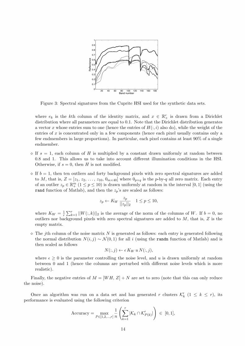
⇧ The spectral signatures of the six endmembers, that is, the columns of W , are taken as the spec-tral signatures of materials from the Cuprite HSI (see Section 3.5.2) and we have W 2 R188⇥6

+ ;see Figure 3. Note that W is rather poorly conditioned ((W ) = 91.5) as the spectral signatureslook very similar to one another.

⇧ The pixels are assigned to the six clusters Kk 1 k r where each cluster contains a di↵erentnumber of pixels with |Kk| = 500� (k � 1)50, 1 k r (for a total of 2250 pixels).

⇧ Once a pixel, say the ith, has been assigned to a cluster, say the kth, the corresponding columnof H is generated as follows:

H(:, i) = 0.9 ek + 0.1x,

2http://www.mathworks.com/matlabcentral/fileexchange/28902-spherical-k-means/content/spkmeans.m

13

20 40 60 80 100 120 140 160 1800

0.1

0.2

0.3

0.4

0.5

0.6

0.7

0.8

0.9

1

Band numberR

efle

ctan

ce

Figure 3: Spectral signatures from the Cuprite HSI used for the synthetic data sets.

where ek is the kth column of the identity matrix, and x 2 Rr+ is drawn from a Dirichlet

distribution where all parameters are equal to 0.1. Note that the Dirichlet distribution generatesa vector x whose entries sum to one (hence the entries of H(:, i) also do), while the weight of theentries of x is concentrated only in a few components (hence each pixel usually contains only afew endmembers in large proportions). In particular, each pixel contains at least 90% of a singleendmember.

⇧ If s = 1, each column of H is multiplied by a constant drawn uniformly at random between0.8 and 1. This allows us to take into account di↵erent illumination conditions in the HSI.Otherwise, if s = 0, then H is not modified.

⇧ If b = 1, then ten outliers and forty background pixels with zero spectral signatures are addedto M , that is, Z = [z1, z2, . . . , z10, 0m⇥40] where 0p⇥q is the p-by-q all zero matrix. Each entryof an outlier zp 2 Rm

+ (1 p 10) is drawn uniformly at random in the interval [0, 1] (using therand function of Matlab), and then the zp’s are scaled as follows:

zp KWzp

||zp||2 1 p 10,

where KW = 1r

Prk=1 ||W (:, k)||2 is the average of the norm of the columns of W . If b = 0, no

outliers nor background pixels with zero spectral signatures are added to M , that is, Z is theempty matrix.

⇧ The jth column of the noise matrix N is generated as follows: each entry is generated followingthe normal distribution N(i, j) ⇠ N (0, 1) for all i (using the randn function of Matlab) and isthen scaled as follows

N(:, j) ✏KW uN(:, j),

where ✏ � 0 is the parameter controlling the noise level, and u is drawn uniformly at randombetween 0 and 1 (hence the columns are perturbed with di↵erent noise levels which is morerealistic).

Finally, the negative entries of M = [WH, Z] +N are set to zero (note that this can only reducethe noise).

Once an algorithm was run on a data set and has generated r clusters K0k (1 k r), its

performance is evaluated using the following criterion

Accuracy = maxP2[1,2,...,r]

1

n

rX

k=1

|Kk \K0P (k)|

!2 [0, 1],

14

where [1, 2, . . . , r] is the set of permutations of {1, 2, . . . , r}, and Kk are the true clusters. Note thatif a data point does not belong to any cluster (such as an outlier), it does not a↵ect the accuracy. Inother words, the accuracy can be equal to 1 even in the presence of outliers (as long as all other datapoints are properly clustered together).

3.3 Results

For each noise level ✏ and each value of s and b, we generate 25 synthetic HSI’s as described inSection 3.2. Figure 4 reports the average accuracy; hence the higher the curve, the better.

Figure 4: Performance of the di↵erent algorithms on synthetic data sets. From top to bottom, left toright: (s, b) = (0, 0), (1,0), (0,1), and (1,1).

We observe that:

⇧ In almost all cases, the hierarchical clustering techniques consistently outperform the plain clus-tering approaches.

⇧ Without scaling nor outliers (top left of Figure 4), HKM performs the best, while H2NMF issecond best.

⇧ With scaling but without outliers (top right of Figure 4), H2NMF performs the best, slightlybetter than SPKM while HKM performs rather poorly. This shows that HKM is sensitive to

15

scaling (that is, to di↵erent illumination conditions in the image), which will be confirmed onthe real-world HSI’s.

⇧ With outliers but without scaling (bottom left of Figure 4), H2NMF outperforms all otheralgorithms. In particular, H2NMF has more than 95% average accuracy for all ✏ 0.3. HSPKMbehaves better than other algorithms but is not able to perfectly cluster the pixels, even for verysmall noise levels.

⇧ With scaling and outliers (bottom right of Figure 4), HKM performs even worse. H2NMF stilloutperforms all other algorithms, while HSPKM extracts relatively good clusters compared tothe other approaches.

Table 1 gives the average computational time (in seconds) of all algorithms for clustering a singlesynthetic data set. We observe that SPKM is significantly faster than all other algorithms while HKMis slightly slower.

H2NMF HKM HSPKM NMF KM SPKM1.68 2.77 1.78 2.25 3.73 0.19

Table 1: Average running time in seconds for the di↵erent algorithms on the synthetic data sets.

3.4 Real-World Hyperspectral Images

In this section, we show that H2NMF is able to perform very good clustering of high resolution real-world HSI’s. This section will focus on illustrating two important contributions: (i) H2NMF performsbetter than standard clustering techniques on real-world HSI, (ii) although H2NMF has been designto deal with HSI’s with pixels dominated mostly by one endmember, it can provide meaningful anduseful results in more di�cult settings, and (iii) H2NMF can be used as an endmember extractionalgorithm in the presence of pure pixels (we compare it to vertex component analysis (VCA) [31] andthe successive projection algorithm (SPA) [3]). Note that because the ground truth of these HSI’s isnot known precisely, it is di�cult to provide an objective quantitative measure for the cluster quality.

3.4.1 H2NMF as an Endmember Extraction Algorithm

Once a set of clustersKk (1 k r) has been identified by H2NMF (or any other clustering technique),each cluster of pixels should roughly correspond to a single material hence M(:,Kk) (1 k r) shouldbe close to rank-one matrices. Therefore, as explained in Section 2.1, it makes sense to approximatethese matrices with their best-rank one approximation: For 1 k r,

M(:,Kk) ⇡ ukvTk , where uk 2 Rm, vk 2 Rn.

Note that, by the Perron-Frobenius and Eckart-Young theorems, uk and vk (1 k r) can be takennonnegative since M is nonnegative. Finally, uk should be close (up to a scaling factor) to the spectralsignature of the endmember corresponding to the kth cluster. To extract a (good) pure pixel, a simplestrategy is therefore to extract a pixel in each Kk whose spectral signature is the closest, with respectto some measure, to uk. In this paper, we use the mean-removed spectral angle (MRSA) betweenuk and the pixels present in the corresponding cluster (see, e.g., [2]). Given two spectral signatures,x, y 2 Rm, it is defined as

�(x, y) =1

⇡arccos

✓(x� x)T (y � y)

||x� x||2||y � y||2

◆2 [0, 1], (3.1)

16

where, for a vector z 2 Rm, z = (Pm

i=1 zi) e and e is the vector of all ones.As we will see, this approach is rather e↵ective for high-resolution images, and much more robust

to noise and outliers than VCA and SPA. This will be illustrated later in this section. (It is importantto keep in mind that SPA and VCA require the pure-pixel assumption while H2NMF requires thatmost pixels are dominated mostly by one endmember.)

3.4.2 Urban HSI

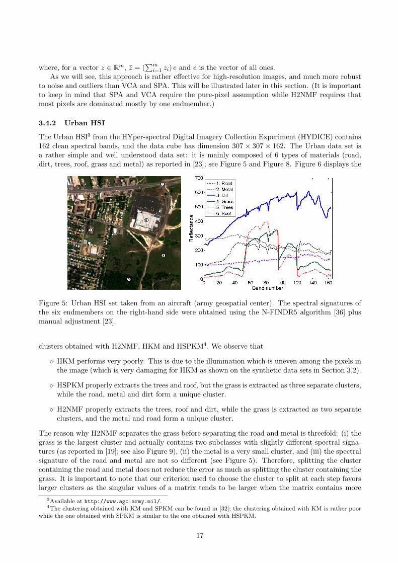
The Urban HSI3 from the HYper-spectral Digital Imagery Collection Experiment (HYDICE) contains162 clean spectral bands, and the data cube has dimension 307 ⇥ 307 ⇥ 162. The Urban data set isa rather simple and well understood data set: it is mainly composed of 6 types of materials (road,dirt, trees, roof, grass and metal) as reported in [23]; see Figure 5 and Figure 8. Figure 6 displays the

Figure 5: Urban HSI set taken from an aircraft (army geospatial center). The spectral signatures ofthe six endmembers on the right-hand side were obtained using the N-FINDR5 algorithm [36] plusmanual adjustment [23].

clusters obtained with H2NMF, HKM and HSPKM4. We observe that

⇧ HKM performs very poorly. This is due to the illumination which is uneven among the pixels inthe image (which is very damaging for HKM as shown on the synthetic data sets in Section 3.2).

⇧ HSPKM properly extracts the trees and roof, but the grass is extracted as three separate clusters,while the road, metal and dirt form a unique cluster.

⇧ H2NMF properly extracts the trees, roof and dirt, while the grass is extracted as two separateclusters, and the metal and road form a unique cluster.

The reason why H2NMF separates the grass before separating the road and metal is threefold: (i) thegrass is the largest cluster and actually contains two subclasses with slightly di↵erent spectral signa-tures (as reported in [19]; see also Figure 9), (ii) the metal is a very small cluster, and (iii) the spectralsignature of the road and metal are not so di↵erent (see Figure 5). Therefore, splitting the clustercontaining the road and metal does not reduce the error as much as splitting the cluster containing thegrass. It is important to note that our criterion used to choose the cluster to split at each step favorslarger clusters as the singular values of a matrix tends to be larger when the matrix contains more

3Available at http://www.agc.army.mil/.4The clustering obtained with KM and SPKM can be found in [32]; the clustering obtained with KM is rather poor

while the one obtained with SPKM is similar to the one obtained with HSPKM.

17

columns (see Section 2.1). Although it works well in many situations (in particular, when clusters arerelatively well balanced), other criterion might be preferable in some cases; this is a topic for furtherresearch.

Figure 7 displays the first levels of the cluster hierarchy generated by H2NMF. We see that if wewere to split the cluster containing the road and metal, they would be properly separated. Therefore,we have also implemented an interactive version of H2NMF (denoted I-H2NMF) where, at each step,the cluster to split is visually selected5. Hence, selecting the right clusters to split (namely, splittingthe road and metal, and not splitting the grass into two clusters) allows us to identifying all materialsseparately, see Figure 8. (Note that this is not possible with HKM and HSPKM.)

Figure 6: Clustering of the Urban HSI. From top to bottom: HKM, HSPKM, and H2NMF.

Using the strategy described in Section 3.4.1, we now compare the di↵erent algorithms when theyare used for endmember extraction. Figure 9 displays the spectral signatures of the pixels extracted bythe di↵erent algorithms. Letting w0

k (1 k r) be the spectral signatures extracted by an algorithm,we match them with the ‘true’ spectral signatures wk (1 k r) from [23] so that

Prk=1 �(wk, w0

k) isminimized; see Equation (3.1). Table 2 reports the MRSA, along with the running time of all methods.Although the hierarchical clustering methods are computationally more expensive, they perform muchbetter than both VCA and SPA.

3.4.3 San Diego Airport

The San Diego airport is a HYDICE HSI containing 158 clean bands, and 400 ⇥ 400 pixels for eachspectral image (i.e., M 2 R158⇥160000

+ ), see Figure 10. There are mainly four types of materials: roadsurfaces, roof, trees and grass; see, e.g., [20]. There are three types of road surfaces including boardingand landing zones, parking lots and streets, and two types of roof tops6. In this section, we performexactly the same experiment as in the previous section for the Urban HSI. The spectral signatures of

5This is also available at https://sites.google.com/site/nicolasgillis/. The user can interactively choose whichcluster to split, when to stop the recursion and, if necessary, which clusters to fuse.

6Note that in [20], only one type of roof top is identified.

18

Figure 7: Hierarchical structure of H2NMF for the Urban HSI.

Figure 8: Interactive H2NMF (I-H2NMF) of the Urban HSI (see also Figure 7). From left to right:grass, trees, roof, dirt, road, and metal.

VCA SPA HKM HSPKM H2NMF I-H2NMFTime (s.) 3.62 1.10 113.79 47.30 41.00 43.18

Road 13.09 11.54 14.97 11.54 7.62 7.27Metal 51.53 62.31 30.72 31.42 28.61 12.74Dirt 60.81 17.35 10.97 13.56 5.08 5.08Grass 16.65 47.32 2.46 2.87 3.39 5.36Trees 53.38 4.21 2.16 1.86 1.63 1.63Roof 26.44 27.40 45.68 8.84 7.30 7.30

Average 36.98 28.36 17.82 11.68 8.94 6.56

Table 2: Running times and MRSA (in percent) for the Urban HSI.

the endmembers are shown on Figure 10 and have been extracted manually using the HYPERACTIVEtoolkit [14].

Figure 11 displays the clusters obtained with H2NMF, HKM and HSPKM. We observe that

19

0 50 100 1500

100

200

300

400

500VCA

Ref

lect

ance

0 50 100 1500

200

400

600

800

1000SPA

0 50 100 1500

200

400

600HKM

0 50 100 1500

200

400

600HSPKM

Ref

lect

ance

Band number0 50 100 150

0

100

200

300

400

500H2NMF

Band number0 50 100 150

0

100

200

300

400

500I−H2NMF

Band number

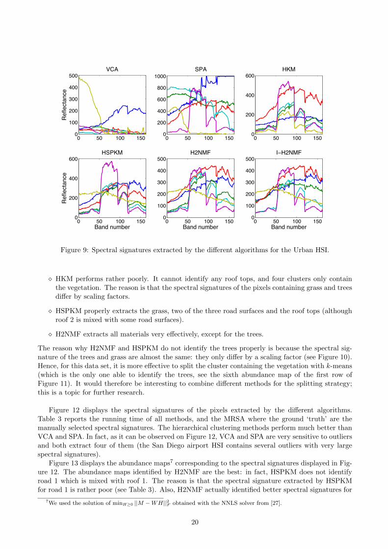
Figure 9: Spectral signatures extracted by the di↵erent algorithms for the Urban HSI.

⇧ HKM performs rather poorly. It cannot identify any roof tops, and four clusters only containthe vegetation. The reason is that the spectral signatures of the pixels containing grass and treesdi↵er by scaling factors.

⇧ HSPKM properly extracts the grass, two of the three road surfaces and the roof tops (althoughroof 2 is mixed with some road surfaces).

⇧ H2NMF extracts all materials very e↵ectively, except for the trees.

The reason why H2NMF and HSPKM do not identify the trees properly is because the spectral sig-nature of the trees and grass are almost the same: they only di↵er by a scaling factor (see Figure 10).Hence, for this data set, it is more e↵ective to split the cluster containing the vegetation with k-means(which is the only one able to identify the trees, see the sixth abundance map of the first row ofFigure 11). It would therefore be interesting to combine di↵erent methods for the splitting strategy;this is a topic for further research.

Figure 12 displays the spectral signatures of the pixels extracted by the di↵erent algorithms.Table 3 reports the running time of all methods, and the MRSA where the ground ‘truth’ are themanually selected spectral signatures. The hierarchical clustering methods perform much better thanVCA and SPA. In fact, as it can be observed on Figure 12, VCA and SPA are very sensitive to outliersand both extract four of them (the San Diego airport HSI contains several outliers with very largespectral signatures).

Figure 13 displays the abundance maps7 corresponding to the spectral signatures displayed in Fig-ure 12. The abundance maps identified by H2NMF are the best: in fact, HSPKM does not identifyroad 1 which is mixed with roof 1. The reason is that the spectral signature extracted by HSPKMfor road 1 is rather poor (see Table 3). Also, H2NMF actually identified better spectral signatures for

7We used the solution of minH�0 ||M �WH||2F obtained with the NNLS solver from [27].

20

0 50 100 1500

1000

2000

3000

4000

5000

6000

7000

8000

9000

Band number

Ref

lect

ance

1. Trees2. Grass3. Roof 14. Roof 25. Road 16. Road 27. Road 3

Figure 10: San Diego airport HSI (left) and manually selected spectral signatures (right).

Figure 11: Clustering of the San Diego airport HSI. From top to bottom: HKM, HSPKM, and H2NMF.

roof 1 and road 1 than the manually selected ones for which the corresponding abundance maps onthe first row of Figure 13 contains more mixture.

Figure 14 displays the first levels of the cluster hierarchy of H2NMF. It is interesting to notice thatroad 2 and 3 can be further split up into two meaningful subclasses. Moreover, another new material isidentified (unknown to us prior to this study), it is some kind of roofing material/dirt (note that HKMand HSPKM are not able to identify this material). Figure 15 displays the clusters obtained usingI-H2NMF, that is, manually splitting and fusing the clusters (more precisely, after having identifiedthe new endmember by splitting road 2, we refuse the two clusters corresponding to road 2); see alsoFigure 14.

21

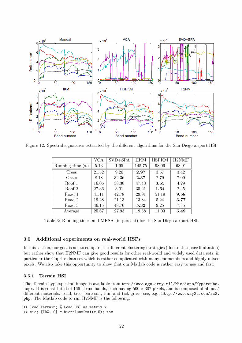
Figure 12: Spectral signatures extracted by the di↵erent algorithms for the San Diego airport HSI.

VCA SVD+SPA HKM HSPKM H2NMFRunning time (s.) 5.13 1.95 145.75 98.09 68.91

Trees 21.52 9.20 2.97 3.57 3.42Grass 8.18 32.36 2.37 2.79 7.09Roof 1 16.06 38.30 47.43 3.55 4.29Roof 2 27.36 3.01 35.21 1.64 2.45Road 1 41.11 42.78 29.91 51.19 9.58Road 2 19.28 21.13 13.84 5.24 3.77Road 3 46.15 48.76 5.32 9.25 7.85Average 25.67 27.93 19.58 11.03 5.49

Table 3: Running times and MRSA (in percent) for the San Diego airport HSI.

3.5 Additional experiments on real-world HSI’s

In this section, our goal is not to compare the di↵erent clustering strategies (due to the space limitation)but rather show that H2NMF can give good results for other real-world and widely used data sets; inparticular the Cuprite data set which is rather complicated with many endmembers and highly mixedpixels. We also take this opportunity to show that our Matlab code is rather easy to use and fast:

3.5.1 Terrain HSI

The Terrain hyperspectral image is available from ttp://www.agc.army.mil/Missions/Hypercube.aspx. It is constituted of 166 cleans bands, each having 500⇥ 307 pixels, and is composed of about 5di↵erent materials: road, tree, bare soil, thin and tick grass; see, e.g., http://www.way2c.com/rs2.php. The Matlab code to run H2NMF is the following:

>> load Terrain; % Load HSI as matrix x

>> tic; [IDX, C] = hierclust2nmf(x,5); toc

22

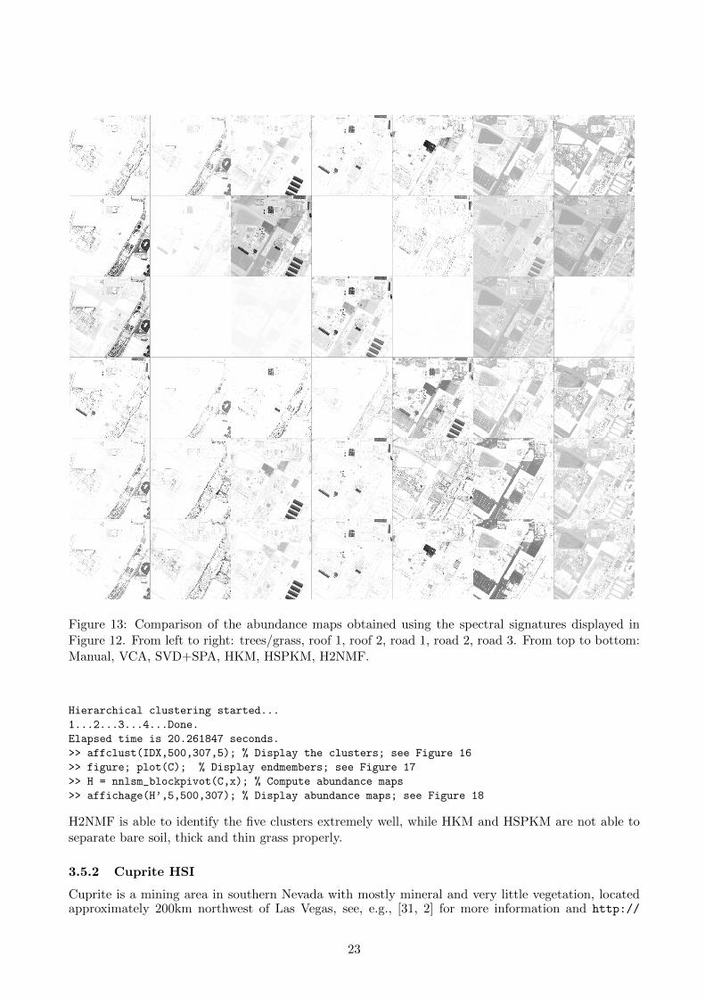
Figure 13: Comparison of the abundance maps obtained using the spectral signatures displayed inFigure 12. From left to right: trees/grass, roof 1, roof 2, road 1, road 2, road 3. From top to bottom:Manual, VCA, SVD+SPA, HKM, HSPKM, H2NMF.

Hierarchical clustering started...

1...2...3...4...Done.

Elapsed time is 20.261847 seconds.

>> affclust(IDX,500,307,5); % Display the clusters; see Figure 16

>> figure; plot(C); % Display endmembers; see Figure 17

>> H = nnlsm_blockpivot(C,x); % Compute abundance maps

>> affichage(H’,5,500,307); % Display abundance maps; see Figure 18

H2NMF is able to identify the five clusters extremely well, while HKM and HSPKM are not able toseparate bare soil, thick and thin grass properly.

3.5.2 Cuprite HSI

Cuprite is a mining area in southern Nevada with mostly mineral and very little vegetation, locatedapproximately 200km northwest of Las Vegas, see, e.g., [31, 2] for more information and http://

23

Figure 14: Hierarchical structure of H2NMF for the San Diego airport HSI.

Figure 15: Clustering of San Diego airport HSI with I-H2NMF. From left to right, top to bottom:vegetation (grass and trees), roof 1, roof 2, road 1, road 2, road 3, dirt/roofing.

Figure 16: Five clusters obtained automatically with H2NMF on the Terrain HSI. From left to right:tree, road, thick grass, bare soil and thin grass.

speclab.cr.usgs.gov/PAPERS.imspec.evol/aviris.evolution.html. It consists of 188 images,each having 250 ⇥ 191 pixels, and is composed of about 20 di↵erent minerals. The Cuprite HSI israther noisy and many pixels are mixture of several endmembers. Hence this experiment illustratesthe usefulness of H2NMF to analyze more di�cult data sets, where the assumption that most pixels

24

Figure 17: Five endmembers obtained with H2NMF on the Terrain HSI.

Figure 18: Five abundance maps corresponding to the endmembers extracted with H2NMF.

are dominated mostly by one endmember is only roughly satisfied; see Figure 19. We run H2NMFwith r = 15:

>> load cuprite_ref; %From www.lx.it.pt/~bioucas.

>> tic; [IDX, C] = hierclust2nmf(x,15); toc

Hierarchical clustering started...

1...2...3...4...5...6...7...8...9...10...

11...12...13...14...Done.

Elapsed time is 11.632038 seconds.

>> affclust(IDX,250,191,5); %See Figure 19 displaying the 15 clusters.

4 Conclusion and Further Work

In this paper, we have introduced a way to perform hierarchical clustering of high-resolution HSI’susing the geometry of such images and the properties of rank-two NMF; see Algorithm 1 (referredto as H2NMF). We showed that the proposed method outperforms k-means, spherical k-means andstandard NMF on several synthetic and real-world data sets, being more robust to noise and outliers,while being computationally very e�cient, requiring O(mnr) operations (m is the number of spectral

25

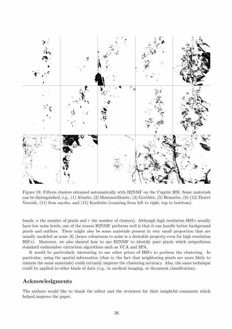
Figure 19: Fifteen clusters obtained automatically with H2NMF on the Cuprite HSI. Some materialscan be distinguished, e.g., (1) Alunite, (2) Montmorillonite, (3) Goethite, (5) Hematite, (8)-(12) DesertVarnish, (11) Iron oxydes, and (15) Kaolinite (counting from left to right, top to botttom).

bands, n the number of pixels and r the number of clusters). Although high resolution HSI’s usuallyhave low noise levels, one of the reason H2NMF performs well is that it can handle better backgroundpixels and outliers. There might also be some materials present in very small proportion that areusually modeled as noise [8] (hence robustness to noise is a desirable property even for high resolutionHSI’s). Moreover, we also showed how to use H2NMF to identify pure pixels which outperformsstandard endmember extraction algorithms such as VCA and SPA.

It would be particularly interesting to use other priors of HSI’s to perform the clustering. Inparticular, using the spatial information (that is, the fact that neighboring pixels are more likely tocontain the same materials) could certainly improve the clustering accuracy. Also, the same techniquecould be applied to other kinds of data (e.g., in medical imaging, or document classification).

Acknowledgments

The authors would like to thank the editor and the reviewers for their insightful comments whichhelped improve the paper.

26

References

[1] Ambikapathi, A., Chan, T.H., Ma, W.K., Chi, C.Y.: A robust alternating volume maximizationalgorithm for endmember extraction in hyperspectral images. In: WHISPERS, Reykjavik, Iceland(2010)

[2] Ambikapathi, A., Chan, T.H., Ma, W.K., Chi, C.Y.: Chance-constrained robust minimum-volumeenclosing simplex algorithm for hyperspectral unmixing. IEEE Trans. Geosci. Remote Sens.49(11), 4194–4209 (2011)

[3] Araujo, U., Saldanha, B., Galvao, R., Yoneyama, T., Chame, H., Visani, V.: The successive pro-jections algorithm for variable selection in spectroscopic multicomponent analysis. Chemometricsand Intelligent Laboratory Systems 57(2), 65–73 (2001)

[4] Arbelaez, P., Maire, M., Fowlkes, C., Malik, J.: Contour detection and hierarchical image seg-mentation. IEEE Trans. on Pattern Analysis and Machine Intelligence 33(5), 898–916 (2011)

[5] Arora, S., Ge, R., Kannan, R., Moitra, A.: Computing a nonnegative matrix factorization –provably. In: STOC ’12, pp. 145–162 (2012)

[6] Banerjee, A., Dhillon, I., Ghosh, J., Sra, S.: Generative model-based clustering of directional data.In: Proceedings of the ninth ACM SIGKDD International Conference on Knowledge Discoveryand Data Mining (KDD-03), pp. 19–28. ACM Press (2003)

[7] Bioucas-Dias, J., Nascimento, J.: Estimation of signal subspace on hyperspectral data. In: Re-mote Sensing, p. 59820L. International Society for Optics and Photonics (2005)

[8] Bioucas-Dias, J., Plaza, A., Dobigeon, N., Parente, M., Du, Q., Gader, P., Chanussot, J.: Hy-perspectral unmixing overview: Geometrical, statistical, and sparse regression-based approaches.IEEE Journal of Selected Topics in Applied Earth Observations and Remote Sensing 5(2), 354–379 (2012)

[9] Cai, D., He, X., Li, Z., Ma, W.Y., Wen, J.R.: Hierarchical clustering of www image search resultsusing visual, textual and link information. In: Proc. of the 12th annual ACM Int. Conf. onMultimedia, pp. 952–959 (2004)

[10] Chan, T.H., Ma, W.K., Ambikapathi, A., Chi, C.Y.: IEEE Trans. Geosci. Remote Sens., title=ASimplex Volume Maximization Framework for Hyperspectral Endmember Extraction, year=2011,volume=49, number=11, pages=4177-4193,

[11] Cohen, J., Rothblum, U.: Nonnegative ranks, Decompositions and Factorization of NonnegativeMatrices. Linear Algebra and its Applications 190, 149–168 (1993)

[12] Eisen, M., Spellman, P., Brown, P., Botstein, D.: Cluster analysis and display of genome-wideexpression patterns. Proc. Natl. Acad. Sci. USA 95(25), 14,863–14,868 (1998)

[13] Faloutsos, C., Lin, K.I.: Fastmap: a fast algorithm for indexing, data-mining and visualizationof traditional and multimedia datasets. In: SIGMOD ’95: Proc. of the 1995 ACM SIGMOD Int.Conf. on Mgmt. of Data, pp. 163–174 (1995)

[14] Fong, M., Hu, Z.: Hyperactive: A matlab tool for visualization of hyperspectral images (2007).http://www.math.ucla.edu/~wittman/lambda/software.html

[15] Gillis, N.: Nonnegative matrix factorization: Complexity, algorithms and applications. Ph.D.thesis, Universite catholique de Louvain (2011)

27

[16] Gillis, N.: Sparse and unique nonnegative matrix factorization through data preprocessing. Jour-nal of Machine Learning Research 13(Nov), 3349–3386 (2012)

[17] Gillis, N.: Robustness analysis of hottopixx, a linear programming model for factoring nonnegativematrices. SIAM J. Mat. Anal. & Appl. 34(3), 1189–1212 (2013)

[18] Gillis, N., Glineur, F.: Accelerated multiplicative updates and hierarchical ALS algorithms fornonnegative matrix factorization. Neural Computation 24(4), 1085–1105 (2012)

[19] Gillis, N., Plemmons, R.: Dimensionality reduction, classification, and spectral mixture analysisusing nonnegative underapproximation. Optical Engineering 50, 027001 (2011)

[20] Gillis, N., Plemmons, R.: Sparse nonnegative matrix underapproximation and its application tohyperspectral image analysis. Linear Algebra and its Applications 438(10), 3991–4007 (2013)

[21] Gillis, N., Vavasis, S.: Fast and robust recursive algorithms for separable nonnegative matrixfactorization. IEEE Trans. Pattern Anal. Mach. Intell. 36(4), 698–714 (2014)

[22] Golub, G., Van Loan, C.: Matrix Computation, 3rd Edition. The Johns Hopkins University PressBaltimore (1996)

[23] Guo, Z., Wittman, T., Osher, S.: L1 unmixing and its application to hyperspectral image en-hancement. In: Proc. SPIE Conference on Algorithms and Technologies for Multispectral, Hy-perspectral, and Ultraspectral Imagery XV (2009)

[24] Jia, S., Qian, Y.: Constrained nonnegative matrix factorization for hyperspectral unmixing. IEEETrans. Geosci. Remote Sens. 47(1), 161–173 (2009)

[25] Kersting, K., Wahabzada, M., Thurau, C., Bauckhage, C.: Hierarchical convex nmf for clusteringmassive data. In: ACML ’10: Proc. of 2nd Asian Conf. on Machine Learning, pp. 253–268 (2010)

[26] Kim, H., Park, H.: Sparse non-negative matrix factorizations via alternating non-negativity-constrained least squares for microarray data analysis. Bioinformatics 23(12), 1495–1502 (2007)

[27] Kim, J., Park, H.: Fast nonnegative matrix factorization: An active-set-like method and com-parisons. SIAM J. on Scientific Computing 33(6), 3261–3281 (2011)

[28] Kuang, D., Park, H.: Fast rank-2 nonnegative matrix factorization for hierarchical documentclustering. In: 19th ACM SIGKDD Conference on Knowledge Discovery and Data Mining (KDD’13), pp. 739–747 (2013)

[29] Li, Y., Sima, D., Van Cauter, S., Croitor Sava, S., Himmelreich, U., Pi, Y., Van Hu↵el, S.:Hierarchical non-negative matrix factorization (hnmf): a tissue pattern di↵erentiation methodfor glioblastoma multiforme diagnosis using mrsi. NMR in Biomedicine 26(3), 307–319 (2012)

[30] Ma, W.K., Bioucas-Dias, J., Chan, T.H., Gillis, N., Gader, P., Plaza, A., Ambikapathi, A., Chi,C.Y.: Signal processing perspective on hyperspectral unmixing. IEEE Signal Processing Magazine31(1), 67–81 (2014)

[31] Nascimento, J., Bioucas-Dias, J.: Vertex component analysis: a fast algorithm to unmix hyper-spectral data. IEEE Trans. Geosci. Remote Sens. 43(4), 898–910 (2005)

[32] Pompili, F., Gillis, N., Absil, P.A., Glineur, F.: Two algorithms for orthogonal nonnegativematrix factorization with application to clustering. Neurocomputing 141, 15–25 (2014)

[33] Ren, H., Chang, C.I.: Automatic spectral target recognition in hyperspectral imagery. IEEETrans. on Aerospace and Electronic Systems 39(4), 1232–1249 (2003)

28

[34] Thomas, L.: Rank factorization of nonnegative matrices. SIAM Review 16(3), 393–394 (1974)

[35] Vavasis, S.: On the complexity of nonnegative matrix factorization. SIAM J. on Optimization20(3), 1364–1377 (2009)

[36] Winter, M.: N-findr: an algorithm for fast autonomous spectral end-member determination inhyperspectral data. In: Proc. SPIE Conference on Imaging Spectrometry V (1999)

[37] Zhao, Y., Karypis, G., Fayyad, U.: Hierarchical clustering algorithms for document datasets.Data Min. Knowl. Discov. 10(2), 141–168 (2005)

[38] Zymnis, A., Kim, S.J., Skaf, J., Parente, M., Boyd, S.: Hyperspectral image unmixing via alter-nating projected subgradients. In: Signals, Systems and Computers, pp. 1164–1168 (2007)

29