Hidden Markov Models in Bioinformatics Applications

CSC391/691 BioinformaticsSpring 2004Fetrow/Burg/Miller(Slides by J. Burg)

How Markov Models Work, In Sketch

Observe the way something has occurred in known cases – for example: the profile of common patterns of amino acids in

a family of proteins the way certain combinations of letters are

pronounced by most people the way certain amino acid sequences typically

fold Use this statistical information to generate

probabilities for future behavior or for other instances whose structure or behavior is unknown.

The Markov Assumption Named after Russian statistician Andrei Markov. Picture a system abstractly as a sequence of states and

associated probabilities that you’ll move from any given state to any of the others.

In a 1st order Markov model, the probability that the system will move to a given state X depends only on the state immediately preceding X. (In a 2nd order chain, it depends on the two previous states, and so forth.)

The independence of one state transition from another is what characterizes the Markov model. It’s called the Markov assumption.

Application of the Markov Assumption to PAM Matrices

The Markov assumption underlies the PAM matrices, modeling the evolution of proteins.

In the PAM matrix design, the probability that amino acid X will mutate to Y is not affected by X’s previous state in evolutionary time.

Markov Model

Defined by a set of states S and the probability of moving from one state to the next.

In computer science language, it’s a stochastic finite state machine.

A Markov sequence is a sequence of states through a given Markov model. It can also be called a Markov chain, or simply a path.

Markov Model

Imagine a weird coin that tends to keep flipping heads once it gets the first head and, not quite so persistently, tails once it gets the first tail.

Review of Probability – Concepts and Notation

P(A) ≡ the probability of A. Note that P(A) ≥ 0 and P(A,B) ≡ the probability that both A and B are true P(A | B) ≡ the probability that A is true given that B

is true = P(A,B) / P(B) P(A,B) = P(A) * P(B) when A and B are

independent events Bayes’ Rule:

P(A | B) = [P(B | A)*P(A)]/P(B)

Aallover

AP 1)(

Hidden Markov Models (HMMs)

A Hidden Markov Model M is defined by a set of states X a set A of transition probabilities between the states, an |

X| x |X| matrix. aij ≡ P(Xj | Xi) The probability of going from state i to state j.

States of X are “hidden” states. an alphabet Σ of symbols emitted in states of X, a set of

emission probabilities E, an X x Σ matrix ei(b) ≡ P(b | Xi). The probability that b is emitted in state i. (Emissions are sometimes called observations.) States “emit” certain symbols according to these

probabilities. Again, it’s a stochastic finite state automaton.

Hidden Markov ModelImagine having two coins, one that is fair and one that is biased infavor of heads. Once the thrower of the coin starts using a particular coin, he tends to continue with that coin. We, the observers, never know whichcoin he is using.

What’s “Hidden” in a Hidden Markov Model? There’s something you can observe (a sequence of observations

O, from Σ) and something you can’t observe directly but that you’ve modeled by the states in M (from the set X).

Example 1: X consists of the states of “raining or not raining” at different moments in time (assuming you can’t look outside for yourself). O consists of observations of someone carrying an umbrella (or not) into the building.

Example 2: The states modeled by M constitute meaningful sentences. The observations in O constitute digital signals produced by human speech.

Example 3: The states in M constitute the structure of a “real” family of proteins. The observations in O constitute the experimentally-determined structure.

Example 4: The states in M model the structure of a “real” family of DNA sequences, divided into genes. The observations in O constitute an experimentally-determined DNA sequence.

Steps for Applying HMMs to MSA

1. A model is constructed consisting of states, an emission vocabulary, transition probabilities, and emission probabilities. For multiple sequence alignment:The emission vocabulary Σ is the set of 20 amino acidsThe states correspond to different regions in the structure of a family of proteins, one column for each such region. In each column, there are three kinds of states: match states (rectangles), insertion states (diamonds), and deletion states (circles). (See next slide.)The match states and insertion states emit amino acids. Deletion states do not.Each position has a probability distribution indicating the probability that each of the amino acids will occur in that position.

States in the HMM for MSA“To understand the relevance of this architecture, imagine a family of proteins with different sequences which have a similar 3D structure….The structure imposes severe constraints on the sequences. For example: The structure might start with an α-helix about 30 aa long, followed by a group that binds to TT dimers, followed by about 20 aa with hydrophobic residues, etc. Basically, we walk along the sequence and enter into different regions in which the probabilities to have different amino acids are different (for example, it is very unlikely for members of the family to have an amino acid with hydrophilic residue in the hydrophobic region, or gly and pro are very likely to be present at sharp bends of the polypeptide chain, etc.). Different columns in the graph correspond to different positions in the 3D structure. Each position has its own probability distribution…giving the probabilities for different amino acids to occur at this position. Each position can be skipped by some members of the family. This is accounted for by the delete states. There might also be members of the family that have additional amino acids relative to the consensus structure. This is allowed by the insertion states.”

From “Multiple Alignment with Hidden Markov Models” by Kalin Vetsigian, http://guava.physics.uiuc.edu/~nigel/courses/498BIO/498BIOonline-essays/hw3/files/HW3-Vetsigian.pdf

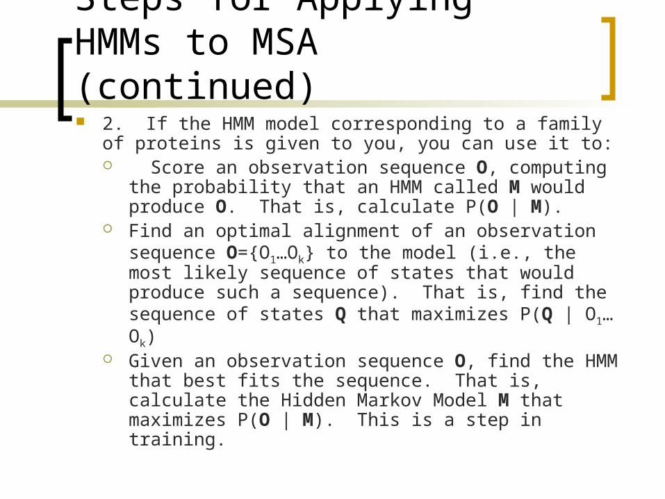
Steps for Applying HMMs to MSA (continued) 2. If the HMM model corresponding to a family of

proteins is given to you, you can use it to: Score an observation sequence O, computing

the probability that an HMM called M would produce O. That is, calculate P(O | M).

Find an optimal alignment of an observation sequence O={O1…Ok} to the model (i.e., the most likely sequence of states that would produce such a sequence). That is, find the sequence of states Q that maximizes P(Q | O1…Ok)

Given an observation sequence O, find the HMM that best fits the sequence. That is, calculate the Hidden Markov Model M that maximizes P(O | M). This is a step in training.

Hidden Markov Model for Multiple Sequence Alignment

From “Multiple Alignment with Hidden Markov Models” by Kalin Vetsigian, http://guava.physics.uiuc.edu/~nigel/courses/498BIO/498BIOonline-essays/hw3/files/HW3-Vetsigian.pdf

Hidden Markov Model for Multiple Sequence Alignment

From “Multiple Alignment with Hidden Markov Models” by Kalin Vetsigian, http://guava.physics.uiuc.edu/~nigel/courses/498BIO/498BIOonline-essays/hw3/files/HW3-Vetsigian.pdf

Steps for Applying HMMs to MSA (continued) 3. If you have to construct the HMM

model from the ground up: The HMM will have a number of

columns equal to the number of amino acids + gaps in the family of proteins.

One way to get the emission and transition probabilities is to begin with a profile alignment for the family of proteins and build the HMM from the profile.

Another way to get the probabilities is to start from scratch and train the HMM.

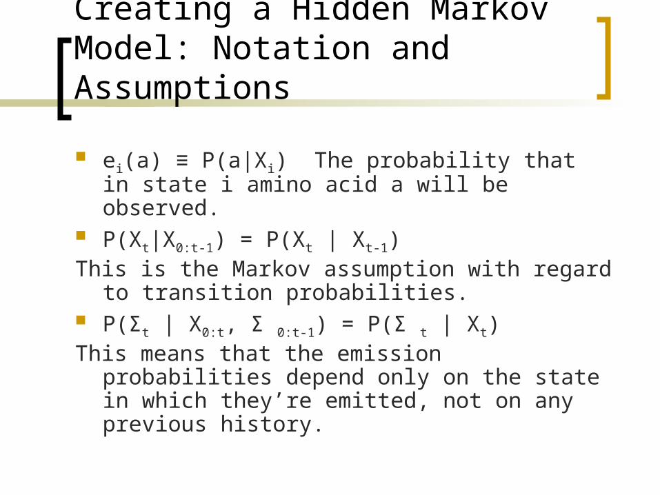
Creating a Hidden Markov Model: Notation and Assumptions

ei(a) ≡ P(a|Xi) The probability that in state i amino acid a will be observed.

P(Xt|X0:t-1) = P(Xt | Xt-1) This is the Markov assumption with regard to

transition probabilities. P(Σt | X0:t, Σ 0:t-1) = P(Σ t | Xt)This means that the emission probabilities

depend only on the state in which they’re emitted, not on any previous history.

Creating a Hidden Markov Model from a Profile

The probabilities for emissions in match states of the HMM will be derived from the frequencies of each amino acid in the respective columns of the profile.

Probabilities for emissions in insertion states will be based on the probability that each amino acid appears anywhere in the sequence.

Delete states don’t need emission probabilities “The transition probabilities between matching and

insertion states can be defined in the affine gap penalty model by assigning aMI, aIM, and aII in such a way that log(aMI) + log(aIM) equals the gap creation penalty and log(aII) equals the gap extension penalty.”

How would you initialize a Hidden Markov Model from this?

Creating a Hidden Markov Model from Scratch

Construct the states as before. Begin with arbitrary transition and emission

probabilities, or hand-chosen ones. Train the model to adjust the probabilities. That is,

calculate the score of each sequence in the training set. Then adjust the probabilities.

Repeat until the training set score can’t be improved any more.

Guaranteed to get a local optimum but not a global one.

To increase the chance of getting a global optimum, try again with different starting values.

Computing Probability that a Certain Emission Sequence Could be Observed by a Given HMM

Compute P(O | M) for O = {O1…Ok}. We don’t know the true state sequence. We must look at all paths that could produce

the sequence O, on the order of NK where N is the number of states.

For even small n and k this is too time-consuming. For N = 5 and K = 100, it would require around 1072 computations.

http://www.it.iitb.ac.in/vweb/engr/cs/dm/Dm_dw/hmmtut.pdfFrom

Forward Recursion

Forward recursion makes the problem more manageable, reducing the computational complexity to on the order of N2

*K operations. The basic idea is not to recompute

parts that are used in more than one term.

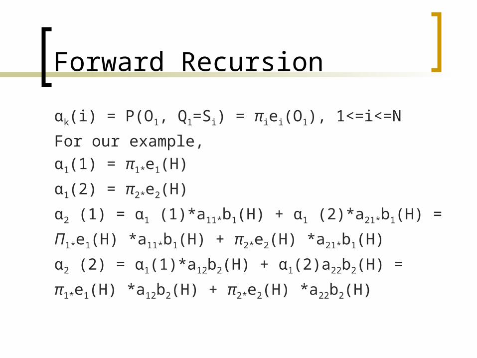
Forward Recursion

αk(i) = P(O1, Q1=Si) = πiei(O1), 1<=i<=N

For our example,

α1(1) = π1*e1(H)

α1(2) = π2*e2(H)

α2 (1) = α1 (1)*a11*b1(H) + α1 (2)*a21*b1(H) =

Π1*e1(H) *a11*b1(H) + π2*e2(H) *a21*b1(H)

α2 (2) = α1(1)*a12b2(H) + α1(2)a22b2(H) =

π1*e1(H) *a12b2(H) + π2*e2(H) *a22b2(H)

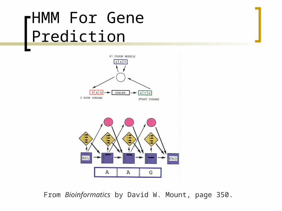
HMM For Gene Prediction

From Bioinformatics by David W. Mount, page 350.