
MapReduce CSE 454 Slides based on those by Jeff Dean, Sanjay Ghemawat, and Dan Weld.
date post
21-Dec-2015Category
view
223download
1
Hidden Markov Models (HMMs)
for Information ExtractionDaniel S. Weld
CSE 454

Extraction with
Finite State Machinese.g.
Hidden Markov Models (HMMs)
standard sequence model in genomics, speech, NLP, …

What’s an HMM?
• Set of states– Initial probabilities– Transition probabilities
• Set of potential observations– Emission probabilities
HMM generates observation sequence
o1 o2 o3 o4 o5
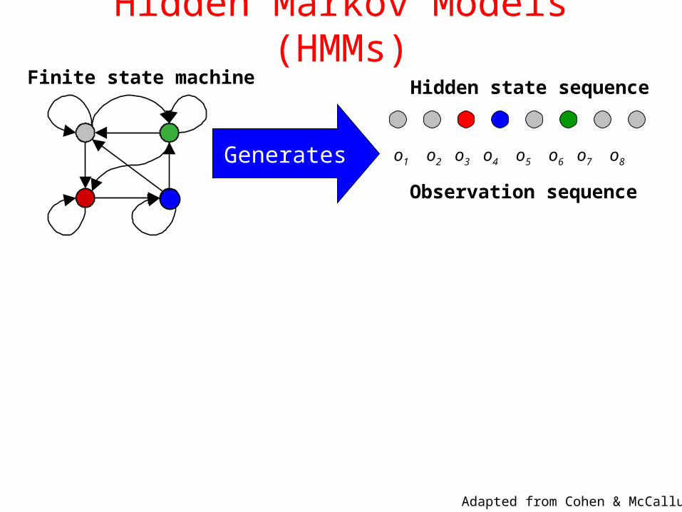
Hidden Markov Models (HMMs)Finite state machine
o1 o2 o3 o4 o5 o6 o7 o8
Hidden state sequence
Observation sequence
Generates
Adapted from Cohen & McCallum

Hidden Markov Models (HMMs)Finite state machine
Graphical Model...Hidden states
Observations
o1 o2 o3 o4 o5 o6 o7 o8
Hidden state sequence
Observation sequence
Generates
Adapted from Cohen & McCallum
yt-2 y
t-1 yt
xt-2 x
t-1x
t...
...
...
Random variable yt takes values from sss{s1, s2, s3, s4} Random variable xt takes values from s{o1, o2, o3, o4, o5, …}

HMMFinite state machine
o1 o2 o3 o4 o5 o6 o7 o8
Hidden state sequence
Observation sequence
Generates
Graphical Model...Hidden states
Observations
yt-2 y
t-1 yt
xt-2 x
t-1x
t...
...
...
Random variable yt takes values from sss{s1, s2, s3, s4} Random variable xt takes values from s{o1, o2, o3, o4, o5, …}

HMMGraphical Model...Hidden states
Observations
yt-2 y
t-1 yt
xt-2 x
t-1x
t...
...
...
Random variable yt takes values from sss{s1, s2, s3, s4} Random variable xt takes values from s{o1, o2, o3, o4, o5, …}
Need Parameters: Start state probabilities: P(y1=sk ) Transition probabilities: P(yt=si | yt-1=sk) Observation probabilities: P(xt=oj | yt=sk )
Training: Maximize probability of training obervations
Usually multinom
ial
over atomic, fixed
alphabet

Example: The Dishonest Casino
A casino has two dice:• Fair die
P(1) = P(2) = P(3) = P(5) = P(6) = 1/6
• Loaded dieP(1) = P(2) = P(3) = P(5) = 1/10P(6) = 1/2
Dealer switches back-&-forth between fair and loaded die about once every 20 turns
Game:1. You bet $12. You roll (always with a fair die)3. Casino player rolls (maybe with
fair die, maybe with loaded die)4. Highest number wins $2
Slides from Serafim Batzoglou

The dishonest casino HMM
FAIR LOADED
0.05
0.05
0.950.95
P(1|F) = 1/6P(2|F) = 1/6P(3|F) = 1/6P(4|F) = 1/6P(5|F) = 1/6P(6|F) = 1/6
P(1|L) = 1/10P(2|L) = 1/10P(3|L) = 1/10P(4|L) = 1/10P(5|L) = 1/10P(6|L) = 1/2
Slides from Serafim Batzoglou

Question # 1 – Evaluation
GIVENA sequence of rolls by the casino player
124552646214614613613666166466163661636616361…
QUESTIONHow likely is this sequence, given our model
of how the casino works?
This is the EVALUATION problem in HMMs
Slides from Serafim Batzoglou

Question # 2 – Decoding
GIVENA sequence of rolls by the casino player
1245526462146146136136661664661636616366163…
QUESTIONWhat portion of the sequence was generated
with the fair die, and what portion with the loaded die?
This is the DECODING question in HMMs
Slides from Serafim Batzoglou

Question # 3 – Learning
GIVENA sequence of rolls by the casino player
124552646214614613613666166466163661636616361651…
QUESTIONHow “loaded” is the loaded die? How “fair” is
the fair die? How often does the casino player change from fair to loaded, and back?
This is the LEARNING question in HMMs
Slides from Serafim Batzoglou

What’s this have to do with Info Extraction?
FAIR LOADED
0.05
0.05
0.950.95
P(1|F) = 1/6P(2|F) = 1/6P(3|F) = 1/6P(4|F) = 1/6P(5|F) = 1/6P(6|F) = 1/6
P(1|L) = 1/10P(2|L) = 1/10P(3|L) = 1/10P(4|L) = 1/10P(5|L) = 1/10P(6|L) = 1/2

What’s this have to do with Info Extraction?
TEXT NAME
0.05
0.05
0.950.95
P(the | T) = 0.003P(from | T) = 0.002…..
P(Dan | N) = 0.005P(Sue | N) = 0.003…

IE with Hidden Markov Models
Yesterday Pedro Domingos spoke this example sentence.
Yesterday Pedro Domingos spoke this example sentence.
Person name: Pedro Domingos
Given a sequence of observations:
and a trained HMM:
Find the most likely state sequence: (Viterbi)
Any words said to be generated by the designated “person name”state extract as a person name:
),(maxarg osPs
person name
location name
background
Slide by Cohen & McCallum

IE with Hidden Markov ModelsFor sparse extraction tasks :• Separate HMM for each type of
target • Each HMM should
– Model entire document– Consist of target and non-target states– Not necessarily fully connected
16Slide by Okan Basegmez

Or … Combined HMM• Example – Research Paper Headers
17Slide by Okan Basegmez

HMM Example: “Nymble”Task: Named Entity Extraction
Train on ~500k words of news wire text.
Case Language F1 .Mixed English 93%Upper English 91%Mixed Spanish 90%
[Bikel, et al 1998], [BBN “IdentiFinder”]
Person
Org
Other
(Five other name classes)
start-of-sentence
end-of-sentence
Results:
Slide adapted from Cohen & McCallum

Finite State Model
Person
Org
Other
(Five other name classes)
start-of-sentence
end-of-sentence
y1
x1 x2 x3
y2 y3 y4 y5 y6 …
x4 x5 x6 …
vs. Path

Question #1 – EvaluationGIVEN
A sequence of observations x1 x2 x3 x4 ……xN
A trained HMM θ=( , , )
QUESTION
How likely is this sequence, given our HMM ?
P(x,θ)Why do we care?
Need it for learning to choose among competing models!

A parse of a sequenceGiven a sequence x = x1……xN,
A parse of o is a sequence of states y = y1, ……, yN
1
2
K
…
1
2
K
…
1
2
K
…
…
…
…
1
2
K
…
x1 x2 x3 xK
2
1
K
2
Slide by Serafim Batzoglou
person
other
location
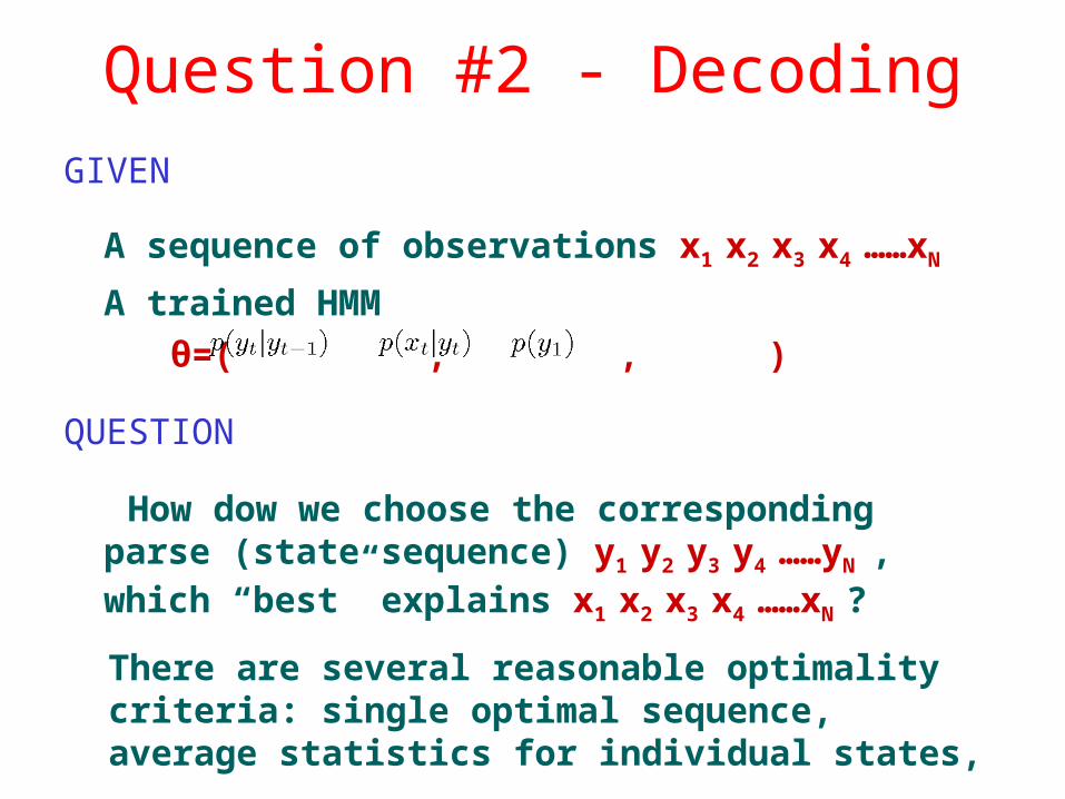
Question #2 - DecodingGIVEN
A sequence of observations x1 x2 x3 x4 ……xN
A trained HMM θ=( , , )
QUESTION
How dow we choose the corresponding parse (state sequence) y1 y2 y3 y4 ……yN , which “best” explains x1 x2 x3 x4 ……xN ?
There are several reasonable optimality criteria: single optimal sequence, average statistics for individual states, …

Question #3 - LearningGIVEN
A sequence of observations x1 x2 x3 x4 ……xN
QUESTION
How do we learn the model parameters
θ =( , , )
which maximize P(x, θ ) ?

Three Questions• Evaluation
– Forward algorithm
• Decoding– Viterbi algorithm
• Learning– Baum-Welch Algorithm (aka “forward-
backward”)– A kind of EM (expectation maximization)

Naive Solution to #1: Evaluation
Given observations x=x1 …xN and HMM θ, what is p(x) ?
Enumerate every possible state sequence y=y1 …yN
Probability of x and given particular y
Probability of particular y
Summing over all possible state sequences we get
NT state sequences!
2T multiplications per sequence
For small HMMsT=10, N=10there are 10
billion sequences!

• Use Dynamic Programming
• Cache and reuse inner sums
“forward variables”
Many Calculations Repeated

Solution to #1: EvaluationUse Dynamic Programming:
Define forward variable
probability that at time t- the state is Si
- the partial observation sequence x=x1 …xt has been emitted

Base Case: Forward Variable t(i)
prob - that the state at t has value Si and
- the partial obs sequence x=x1 …xt has been seen
1
2
K
…
x1
person
other
location
Base Case: t=1 1(i) = p(y1=Si) p(x1=o1)

Inductive Case: Forward Variable t(i)
prob - that the state at t has value Si and
- the partial obs sequence x=x1 …xt has been seen
1
2
K
…
1
2
K
…
1
2
K
…
…
…
…
1
2
K
…
x1 x2 x3
person
other
location
…
…
…
xt
Si

The Forward Algorithm
yt-1 yt
t-1(1)
t-1(2)
t-1(3)
t-1(K)
t(3)
SK SK

The Forward Algorithm
INITIALIZATION
INDUCTION
TERMINATION
Time:O(K2N)
Space:O(KN)
K = |S| #statesN length of sequence

The Backward Algorithm

Three Questions• Evaluation
– Forward algorithm– (also Backward algorithm)
• Decoding– Viterbi algorithm
• Learning– Baum-Welch Algorithm (aka “forward-
backward”)– A kind of EM (expectation maximization)

#2 – Decoding ProblemGiven x=x1 …xN and HMM θ, what is “best”
parse y1 …yT?
Several possible meanings of ‘solution’1. States which are individually most likely2. Single best state sequence
We want sequence y1 …yT, such that P(x,y) is maximized
y* = argmaxy P( x, y )
Again, we can use dynamic programming!
1
2
K
…
1
2
K
…
1
2
K
…
…
…
…
1
2
K
…
o1 o2 o3 oT
2
1
K
2
? ? ? ? ? ? ? ?

δt(i) • Like
t(i) = prob that the state, y, at time t has value Si
and the partial obs sequence x=x1 …xt has been seen
• Defineδt(i) = probability of most likely state sequence
ending with state Si, given observations x1, …, xt
P(y1, …,yt-1 , yt=Si | o1, …, ot, )

δt(i) = probability of most likely
state sequence ending with state Si,
given observations x1, …, xt
P(y1, …,yt-1 , yt=Si | o1, …, ot, )
Base Case: t=1
Maxi P(y1=Si) P(x1=o1 | y1 = Si)
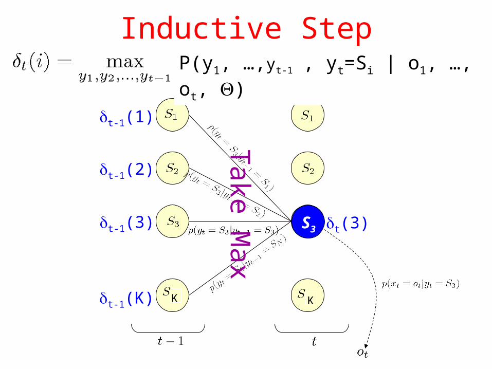
Inductive StepP(y1, …,yt-1 , yt=Si | o1, …, ot, )
t-1(1)
t-1(2)
t-1(3)
t-1(K) K K
t(3)
Take
Max
S3

The Viterbi AlgorithmDEFINE
INITIALIZATION
INDUCTION
TERMINATION
Backtracking to get state sequence y*
| o1, …, ot,

Slides from Serafim Batzoglou
The Viterbi Algorithmx1 x2 ……xj-1 xj……………………………..xT
State 1
2
K
i δj(i)
Maxi δj-1(i) * Ptrans* Pobs
Remember: δt(i) = probability of most likely state seq ending with yt = state St

Terminating Viterbi
δ
δ
δ
δ
δ
x1 x2 …………………………………………..xT
State 1
2
K
i Choose Max

Terminating Viterbi
Time: O(K2T)Space: O(KT)
x1 x2 …………………………………………..xT
State 1
2
K
i
Linear in length of sequence
Maxi δT-1(i) * Ptrans* Pobs
Max
How did we compute *?
δ*
Now Backchain to Find Final Sequence

The Viterbi Algorithm
44
Pedro Domingos

Three Questions• Evaluation
– Forward algorithm– (Could also go other direction)
• Decoding– Viterbi algorithm
• Learning– Baum-Welch Algorithm (aka “forward-
backward”)– A kind of EM (expectation maximization)

• If we have labeled training data!• Input:
Solution to #3 - Learning
person name
location name
background
• Output:– Initial state & transition probabilities:
p(y1), p(yt|yt-1)
– Emission probabilities: p(xt | yt)
}states & edges, butno probabilities
Yesterday Pedro Domingos spoke this example sentence.Many labeled sentences

• Input:
Supervised Learningperson name
location name
background
• Output:– Initial state probabilities: p(y1)
• P(y1=name) = 1/4
• P(y1=location) = 1/4
• P(y1=background) = 2/4
}states & edges, butno probabilities
Yesterday Pedro Domingos spoke this example sentence.Daniel Weld gave his talk in Mueller 153.Sieg 128 is a nasty lecture hall, don’t you think?The next distinguished lecture is by Oren Etzioni on Thursday.

• Input:
Supervised Learningperson name
location name
background
• Output:– State transition probabilities: p(yt|yt-1)
• P(yt=name | yt-1=name) =
• P(yt=name | yt-1=background) =
• Etc…
}states & edges, butno probabilities
Yesterday Pedro Domingos spoke this example sentence.Daniel Weld gave his talk in Mueller 153.Sieg 128 is a nasty lecture hall, don’t you think?The next distinguished lecture is by Oren Etzioni on Thursday.
3/62/22

• Input:
Supervised Learningperson name
location name
background
• Output:– Initial state probabilities: p(y1), p(yt|yt-1)
– Emission probabilities: p(xt | yt)
}states & edges, butno probabilities
Yesterday Pedro Domingos spoke this example sentence.Many labeled sentences

• Input:
Supervised Learningperson name
location name
background
• Output:– Initial state probabilities: p(y1), p(yt|yt-1)
– Emission probabilities: p(xt | yt)
}states & edges, butno probabilities
Yesterday Pedro Domingos spoke this example sentence.Many labeled sentences

Solution to #3 - LearningGiven x1 …xN , how do we learn θ =( , , ) to
maximize P(x)?
• Unfortunately, there is no known way to analytically find a global maximum θ * such that
θ * = arg max P(o | θ)
• But it is possible to find a local maximum; given an initial model θ, we can always find a model θ’ such that
P(o | θ’) ≥ P(o | θ)

52
Chicken & Egg Problem• If we knew the actual sequence of states
– It would be easy to learn transition and emission probabilities
– But we can’t observe states, so we don’t!
• If we knew transition & emission probabilities– Then it’d be easy to estimate the sequence of states
(Viterbi)– But we don’t know them!
Slide by Daniel S. Weld

53
Simplest Version• Mixture of two distributions
• Know: form of distribution & variance,% =5
• Just need mean of each distribution.01 .03 .05 .07 .09
Slide by Daniel S. Weld

54
Input Looks Like
.01 .03 .05 .07 .09
Slide by Daniel S. Weld

55
We Want to Predict
.01 .03 .05 .07 .09
?
Slide by Daniel S. Weld

56
Chicken & Egg
.01 .03 .05 .07 .09
Note that coloring instances would be easy
if we knew Gausians….
Slide by Daniel S. Weld

57
Chicken & Egg
.01 .03 .05 .07 .09
And finding the Gausians would be easy
If we knew the coloring
Slide by Daniel S. Weld

58
Expectation Maximization (EM)
• Pretend we do know the parameters
– Initialize randomly: set 1=?; 2=?
.01 .03 .05 .07 .09
Slide by Daniel S. Weld

59
Expectation Maximization (EM)• Pretend we do know the parameters
– Initialize randomly• [E step] Compute probability of instance
having each possible value of the hidden variable
.01 .03 .05 .07 .09
Slide by Daniel S. Weld

60
Expectation Maximization (EM)• Pretend we do know the parameters
– Initialize randomly• [E step] Compute probability of instance
having each possible value of the hidden variable
.01 .03 .05 .07 .09
Slide by Daniel S. Weld

61
Expectation Maximization (EM)• Pretend we do know the parameters
– Initialize randomly• [E step] Compute probability of instance
having each possible value of the hidden variable
.01 .03 .05 .07 .09
[M step] Treating each instance as fractionally having both values compute the new parameter values
Slide by Daniel S. Weld

62
ML Mean of Single Gaussian
Uml = argminu i(xi – u)2
.01 .03 .05 .07 .09
Slide by Daniel S. Weld

63
Expectation Maximization (EM)
• [E step] Compute probability of instance having each possible value of the hidden variable
.01 .03 .05 .07 .09
[M step] Treating each instance as fractionally having both values compute the new parameter values
Slide by Daniel S. Weld

64
Expectation Maximization (EM)
• [E step] Compute probability of instance having each possible value of the hidden variable
.01 .03 .05 .07 .09
Slide by Daniel S. Weld

65
Expectation Maximization (EM)
• [E step] Compute probability of instance having each possible value of the hidden variable
.01 .03 .05 .07 .09
[M step] Treating each instance as fractionally having both values compute the new parameter values
Slide by Daniel S. Weld
66
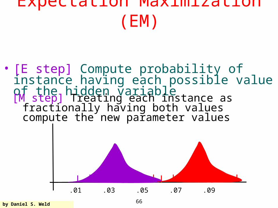
Expectation Maximization (EM)
• [E step] Compute probability of instance having each possible value of the hidden variable
.01 .03 .05 .07 .09
[M step] Treating each instance as fractionally having both values compute the new parameter values
Slide by Daniel S. Weld

67
EM for HMMs [E step] Compute probability of instance
having each possible value of the hidden variable– Compute the forward and backward probabilities
for given model parameters and our observations
[M step] Treating each instance as fractionally having every value compute the new parameter values
- Re-estimate the model parameters - Simple counting

Summary - Learning• Use hill-climbing
– Called the Baum/Welch algorithm– Also “forward-backward algorithm”
• Idea– Use an initial parameter instantiation– Loop
• Compute the forward and backward probabilities for given model parameters and our observations
• Re-estimate the parameters
– Until estimates don’t change much

The Problem with HMMs• We want more than an Atomic View
of Words• We want many arbitrary, overlapping
features of words
identity of wordends in “-ski”is capitalizedis part of a noun phraseis in a list of city namesis under node X in WordNetis in bold fontis indentedis in hyperlink anchorlast person name was femalenext two words are “and Associates”
yt -1
yt
xt
yt+1
xt +1
xt -1
…
…part of
noun phrase
is “Wisniewski”
ends in “-ski”
Slide by Cohen & McCallum

Problems with the Joint ModelThese arbitrary features are not independent.
– Multiple levels of granularity (chars, words, phrases)
– Multiple dependent modalities (words, formatting, layout)
– Past & future
Two choices:
Model the dependencies.Each state would have its own Bayes Net. But we are already starved for training data!
Ignore the dependencies.This causes “over-counting” of evidence (ala naïve Bayes). Big problem when combining evidence, as in Viterbi!
St -1
St
Ot
St+1
Ot +1
Ot -1
St -1
St
Ot
St+1
Ot +1
Ot -1Slide by Cohen & McCallum

Discriminative vs. Generative Models
• So far: all models generative• Generative Models …
model P(y, x)• Discriminative Models …
model P(y | x)
P(y|x) does not include a model of P(x), so it does not need to model the dependencies between features!

Discriminative Models often better• Eventually, what we care about is p(y|x)!
– Bayes Net describes a family of joint distributions of, whose conditionals take certain form
– But there are many other joint models, whose conditionals also have that form.
• We want to make independence assumptions among y, but not among x.

Conditional Sequence Models• We prefer a model that is trained to
maximize a conditional probability rather than joint probability:
P(y|x) instead of P(y,x):
– Can examine features, but not responsible for generating them.
– Don’t have to explicitly model their dependencies.
– Don’t “waste modeling effort” trying to generate what we are given at test time anyway.
Slide by Cohen & McCallum

Finite State Models
Naïve Bayes
Logistic Regression
Linear-chain CRFs
HMMsGenerative
directed models
General CRFs
Sequence
Sequence
Conditional Conditional Conditional
GeneralGraphs
GeneralGraphs

Linear-Chain Conditional Random Fields
• Conditional p(y|x) that follows from joint p(y,x) of HMM is a linear CRF with certain feature functions!

Linear-Chain Conditional Random Fields
• Definition:A linear-chain CRF is a distribution that takes the form
where Z(x) is a normalization function
parameters
feature functions

Linear-ChainConditional Random Fields
• HMM-like linear-chain CRF
• Linear-chain CRF, in which transition score depends on the current observation
…
…x
y
…
…x
y


