Hidden Markov Models CMSC 723: Computational Linguistics I ― Session #5 Jimmy Lin The iSchool...
70
Hidden Markov Models CMSC 723: Computational Linguistics I ― Session #5 Jimmy Lin The iSchool University of Maryland Wednesday, September 30, 2009
-
date post
22-Dec-2015 -
Category
Documents
-
view
222 -
download
1
Transcript of Hidden Markov Models CMSC 723: Computational Linguistics I ― Session #5 Jimmy Lin The iSchool...
Hidden Markov ModelsCMSC 723: Computational Linguistics I ― Session #5
Jimmy LinThe iSchoolUniversity of Maryland
Wednesday, September 30, 2009
Today’s Agenda The great leap forward in NLP
Hidden Markov models (HMMs) Forward algorithm Viterbi decoding Supervised training Unsupervised training teaser
HMMs for POS tagging
Deterministic to Stochastic The single biggest leap forward in NLP:
From deterministic to stochastic models What? A stochastic process is one whose behavior is non-
deterministic in that a system’s subsequent state is determined both by the process’s predictable actions and by a random element.
What’s the biggest challenge of NLP?
Why are deterministic models poorly adapted?
What’s the underlying mathematical tool?
Why can’t you do this by hand?
FSM: Formal Specification Q: a finite set of N states
Q = {q0, q1, q2, q3, …}
The start state: q0
The set of final states: qF
Σ: a finite input alphabet of symbols
δ(q,i): transition function Given state q and input symbol i, transition to new state q'
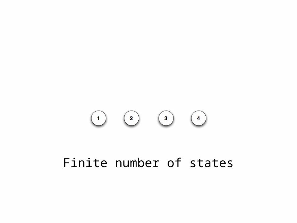
Finite number of states
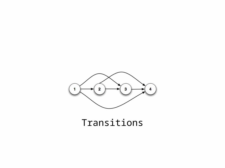
Transitions
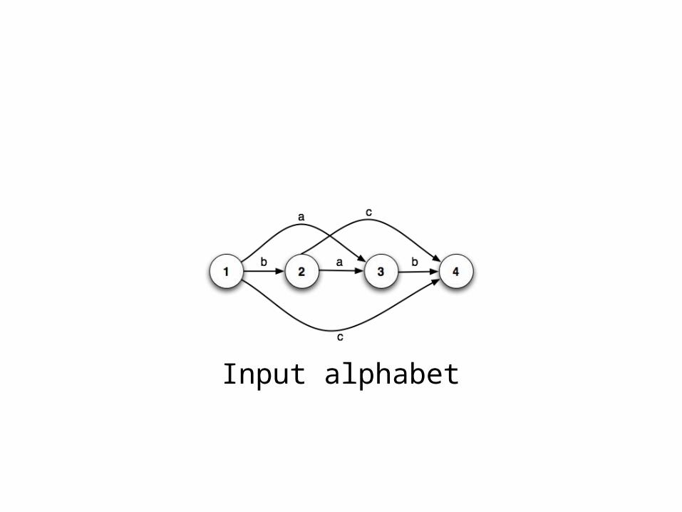
Input alphabet
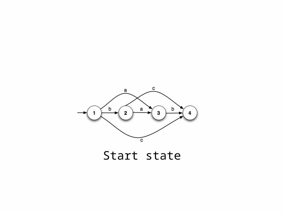
Start state
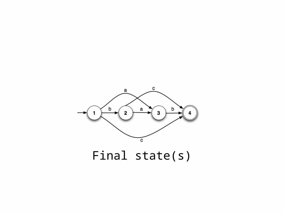
Final state(s)
The problem with FSMs… All state transitions are equally likely
But what if we know that isn’t true?
How might we know?
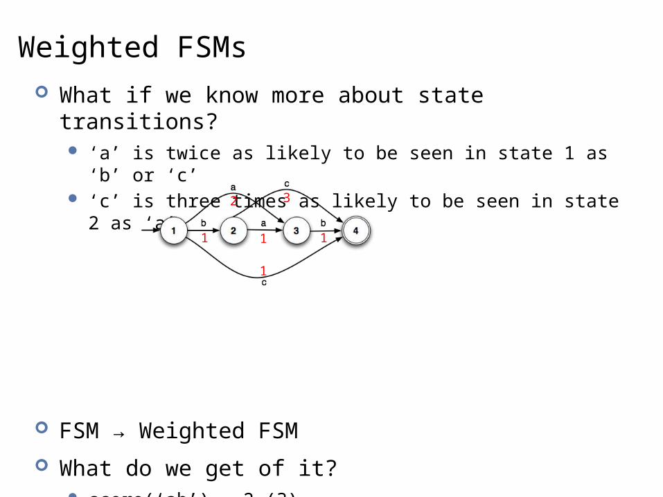
Weighted FSMs What if we know more about state transitions?
‘a’ is twice as likely to be seen in state 1 as ‘b’ or ‘c’ ‘c’ is three times as likely to be seen in state 2 as ‘a’
FSM → Weighted FSM
What do we get of it? score(‘ab’) = 2 (?) score(‘bc’) = 3 (?)
2
1
1
1
3
1
Introducing Probabilities What’s the problem with adding weights to transitions?
What if we replace weights with probabilities? Probabilities provide a theoretically-sound way to model
uncertainly (ambiguity in language) But how do we assign probabilities?
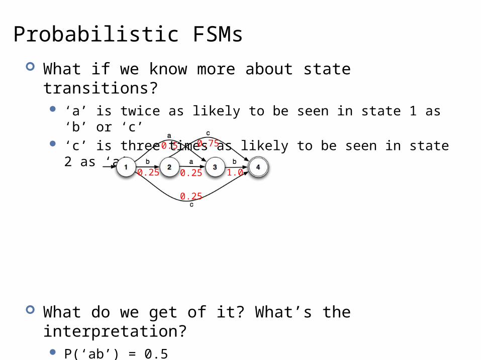
Probabilistic FSMs What if we know more about state transitions?
‘a’ is twice as likely to be seen in state 1 as ‘b’ or ‘c’ ‘c’ is three times as likely to be seen in state 2 as ‘a’
What do we get of it? What’s the interpretation? P(‘ab’) = 0.5 P(‘bc’) = 0.1875
This is a Markov chain
0.5
0.25
0.25
0.25
0.75
1.0
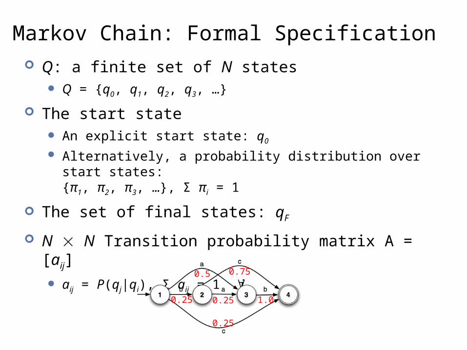
Markov Chain: Formal Specification Q: a finite set of N states
Q = {q0, q1, q2, q3, …}
The start state An explicit start state: q0
Alternatively, a probability distribution over start states:{π1, π2, π3, …}, Σ πi = 1
The set of final states: qF
N N Transition probability matrix A = [aij]
aij = P(qj|qi), Σ aij = 1 i
0.5
0.25
0.25
0.25
0.75
1.0
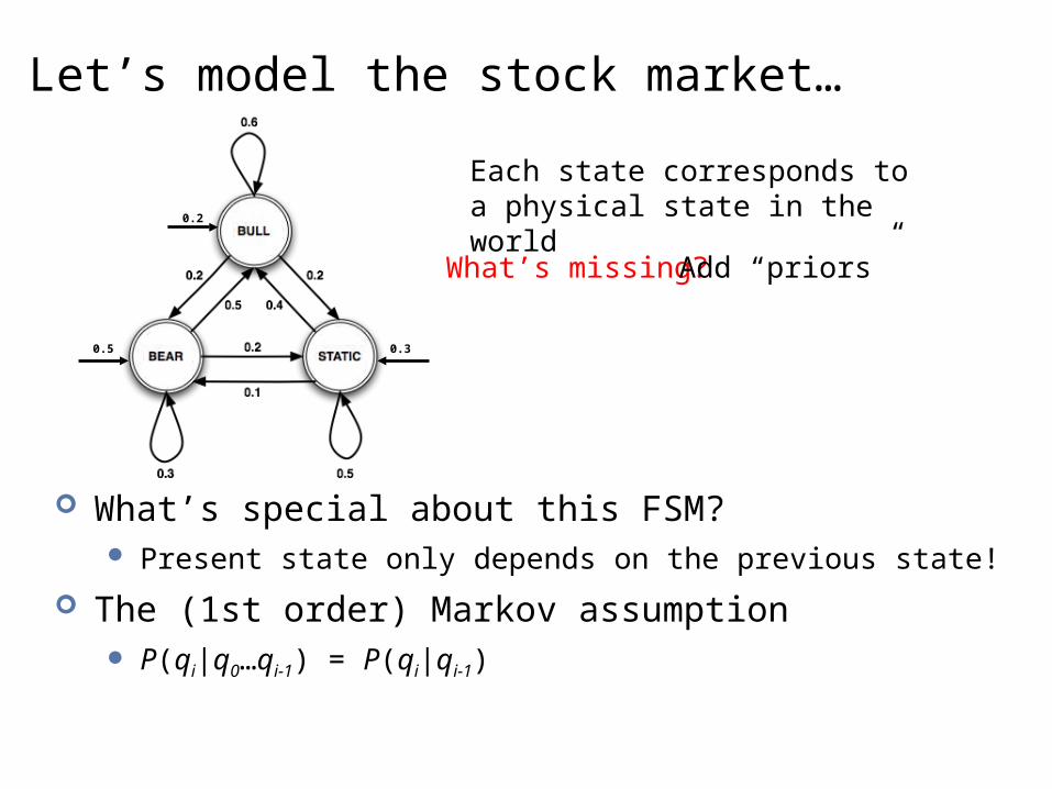
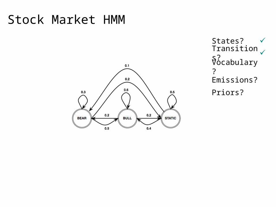
Let’s model the stock market…
What’s special about this FSM? Present state only depends on the previous state!
The (1st order) Markov assumption P(qi|q0…qi-1) = P(qi|qi-1)
0.2
0.5 0.3
What’s missing? Add “priors”
Each state corresponds to a physical state in the world
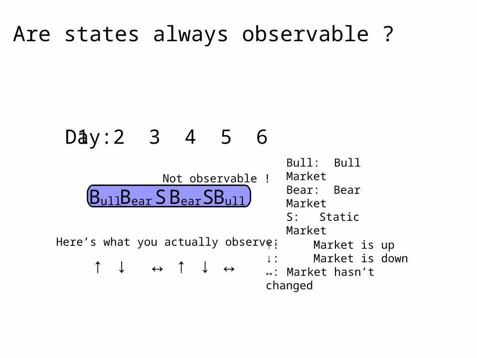
Are states always observable ?
1 2 3 4 5 6Day:
↑ ↓ ↔ ↑ ↓ ↔↑: Market is up↓: Market is down↔: Market hasn’t changed
BullBearSBear BullSBull: Bull MarketBear: Bear MarketS: Static Market
Not observable !
Here’s what you actually observe:
Hidden Markov Models Markov chains aren’t enough!
What if you can’t directly observe the states? We need to model problems where observations don’t directly
correspond to states…
Solution: A Hidden Markov Model (HMM) Assume two probabilistic processes Underlying process (state transition) is hidden Second process generates sequence of observed events
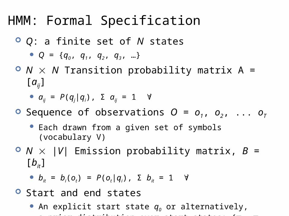
HMM: Formal Specification Q: a finite set of N states
Q = {q0, q1, q2, q3, …}
N N Transition probability matrix A = [aij]
aij = P(qj|qi), Σ aij = 1 i
Sequence of observations O = o1, o2, ... oT
Each drawn from a given set of symbols (vocabulary V)
N |V| Emission probability matrix, B = [bit]
bit = bi(ot) = P(ot|qi), Σ bit = 1 i
Start and end states An explicit start state q0 or alternatively,
a prior distribution over start states: {π1, π2, π3, …}, Σ πi = 1
The set of final states: qF

Stock Market HMM
States? ✓
Transitions?
Vocabulary?
Emissions?
Priors?
Stock Market HMM
States? ✓
Transitions? ✓
Vocabulary?
Emissions?
Priors?
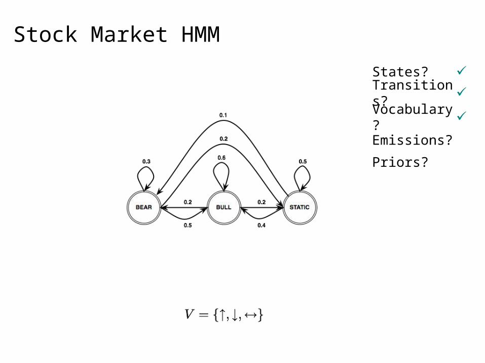
Stock Market HMM
States? ✓
Transitions? ✓
Vocabulary? ✓
Emissions?
Priors?
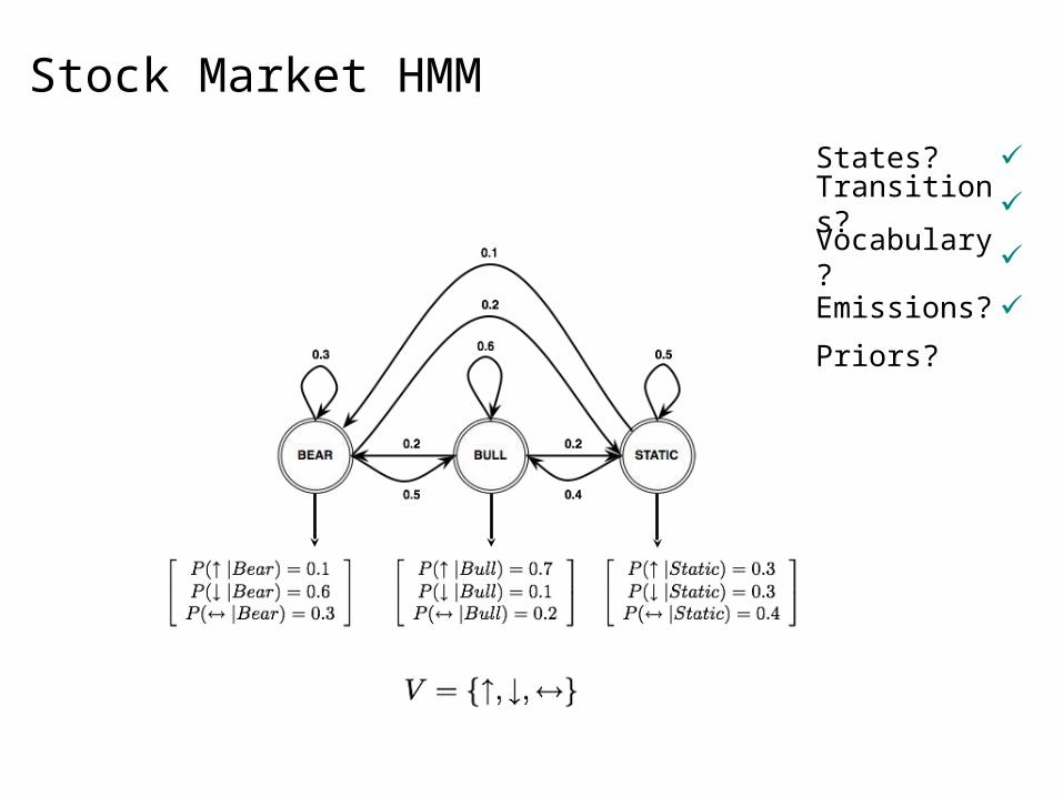
Stock Market HMM
States? ✓
Transitions? ✓
Vocabulary? ✓
Emissions?
Priors?
✓
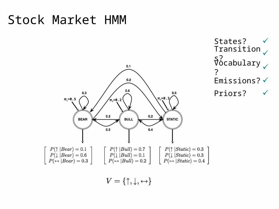
Stock Market HMM
π1=0.5 π2=0.2 π3=0.3
States? ✓
Transitions? ✓
Vocabulary? ✓
Emissions?
Priors?
✓
✓
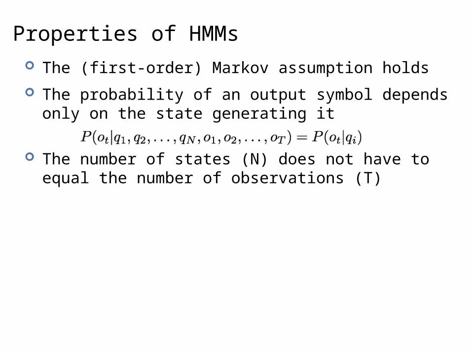
Properties of HMMs The (first-order) Markov assumption holds
The probability of an output symbol depends only on the state generating it
The number of states (N) does not have to equal the number of observations (T)
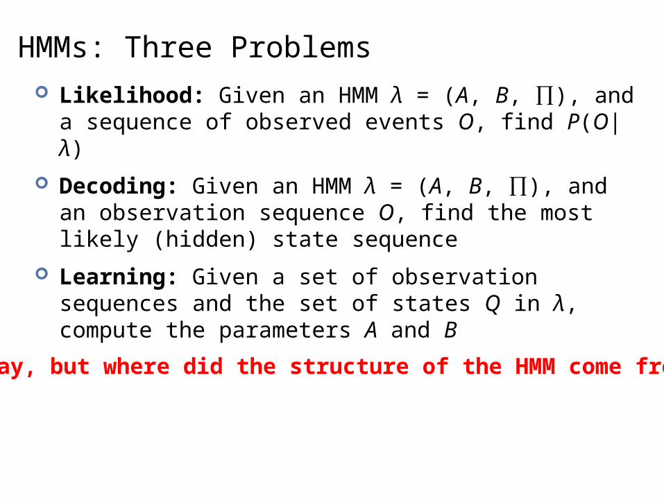
HMMs: Three Problems Likelihood: Given an HMM λ = (A, B, ∏), and a sequence
of observed events O, find P(O|λ)
Decoding: Given an HMM λ = (A, B, ∏), and an observation sequence O, find the most likely (hidden) state sequence
Learning: Given a set of observation sequences and the set of states Q in λ, compute the parameters A and B
Okay, but where did the structure of the HMM come from?
HMM Problem #1: Likelihood
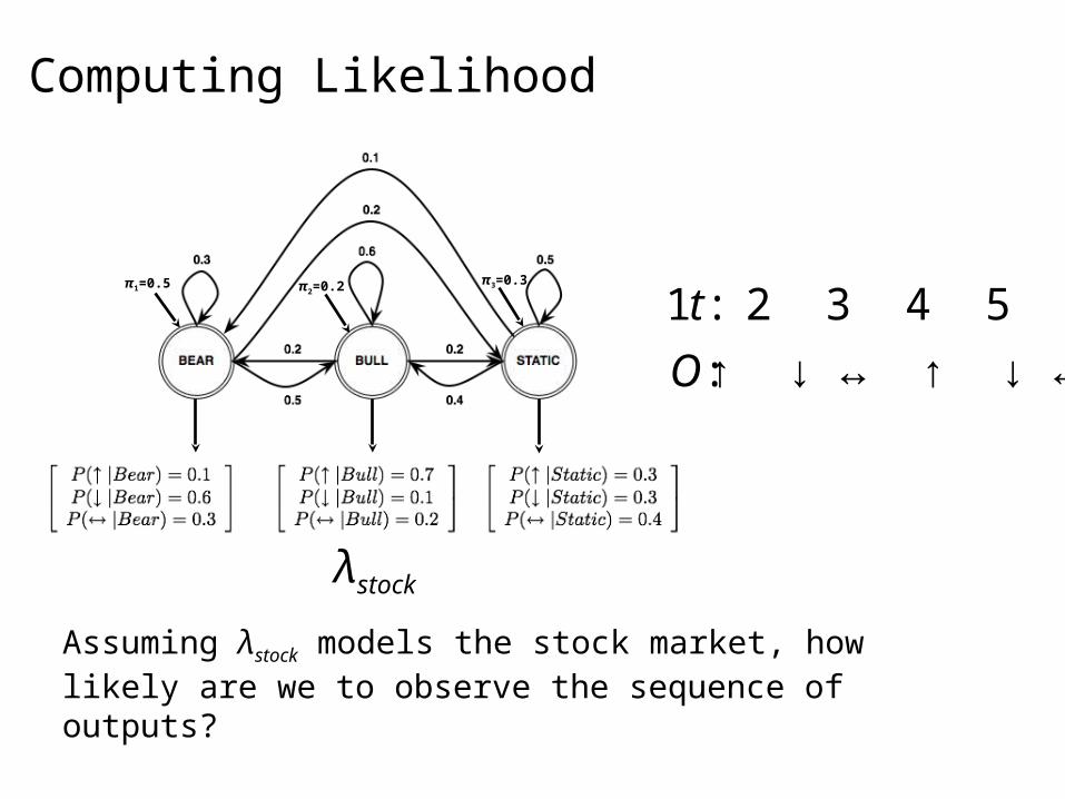
Computing Likelihood
1 2 3 4 5 6t:
↑ ↓ ↔ ↑ ↓ ↔O:
λstock
Assuming λstock models the stock market, how likely are we to observe the sequence of outputs?
π1=0.5 π2=0.2 π3=0.3
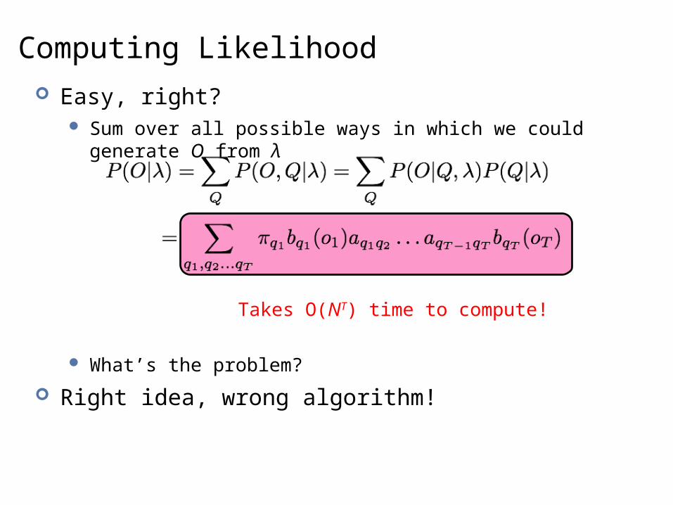
Computing Likelihood Easy, right?
Sum over all possible ways in which we could generate O from λ
What’s the problem?
Right idea, wrong algorithm!Takes O(NT) time to compute!
Computing Likelihood What are we doing wrong?
State sequences may have a lot of overlap… We’re recomputing the shared subsequences every time Let’s store intermediate results and reuse them! Can we do this?
Sounds like a job for dynamic programming!
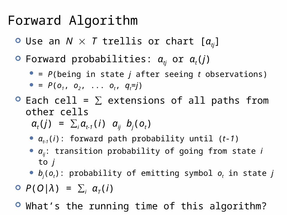
Forward Algorithm Use an N T trellis or chart [αtj]
Forward probabilities: αtj or αt(j) = P(being in state j after seeing t observations) = P(o1, o2, ... ot, qt=j)
Each cell = ∑ extensions of all paths from other cells αt(j) = ∑i αt-1(i) aij bj(ot)
αt-1(i): forward path probability until (t-1)
aij: transition probability of going from state i to j
bj(ot): probability of emitting symbol ot in state j
P(O|λ) = ∑i αT(i)
What’s the running time of this algorithm?
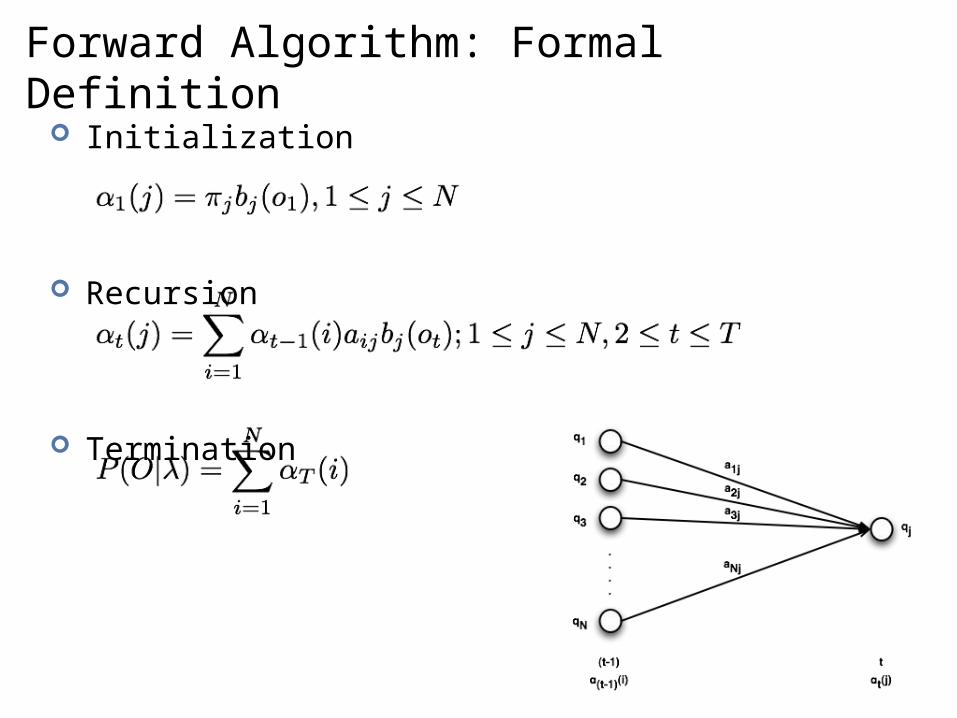
Forward Algorithm: Formal Definition Initialization
Recursion
Termination
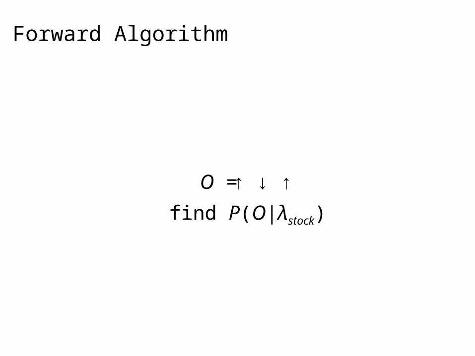
Forward Algorithm
↑ ↓ ↑O =
find P(O|λstock)
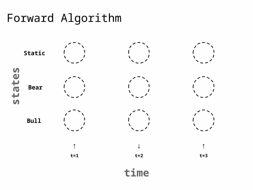
Forward Algorithm
time
↑ ↓ ↑t=1 t=2 t=3
Bear
Bull
Static
stat
es
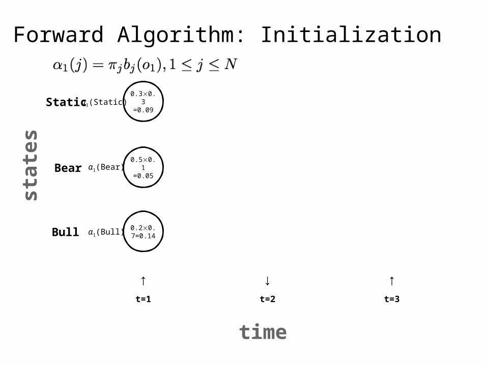
Forward Algorithm: Initialization
α1(Bull)
α1(Bear)
α1(Static)
time
↑ ↓ ↑t=1 t=2 t=3
0.20.7=0.14
0.50.1=0.05
0.30.3=0.09
Bear
Bull
Static
stat
es
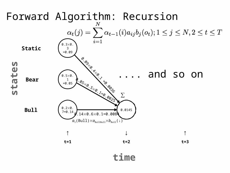
Forward Algorithm: Recursion
0.140.60.1=0.0084
0.050.50.1=0.0025
0.090.40.1 =0.0036
∑
α1(Bull)aBullBullbBull(↓)
.... and so on
time
↑ ↓ ↑t=1 t=2 t=3
0.20.7=0.14
0.50.1=0.05
0.30.3=0.09
0.0145
Bear
Bull
Static
stat
es
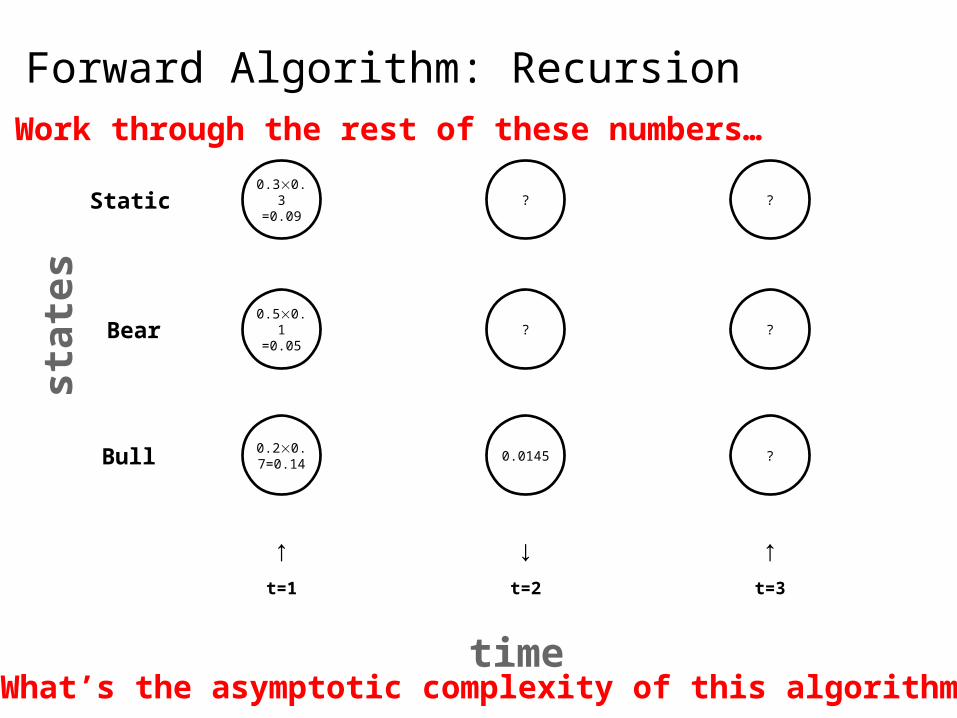
Forward Algorithm: Recursion
time
↑ ↓ ↑t=1 t=2 t=3
0.20.7=0.14
0.50.1=0.05
0.30.3=0.09
0.0145
?
?
?
?
?
Bear
Bull
Static
stat
es
Work through the rest of these numbers…
What’s the asymptotic complexity of this algorithm?
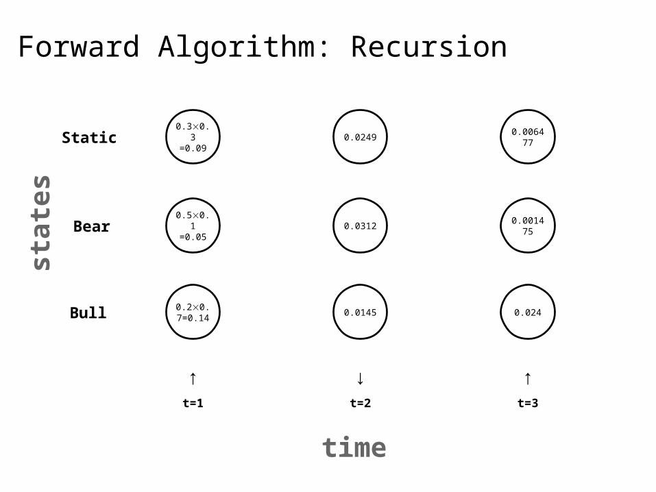
Forward Algorithm: Recursion
time
↑ ↓ ↑t=1 t=2 t=3
0.20.7=0.14
0.50.1=0.05
0.30.3=0.09
0.0145
0.0312
0.0249
0.024
0.001475
0.006477
Bear
Bull
Static
stat
es
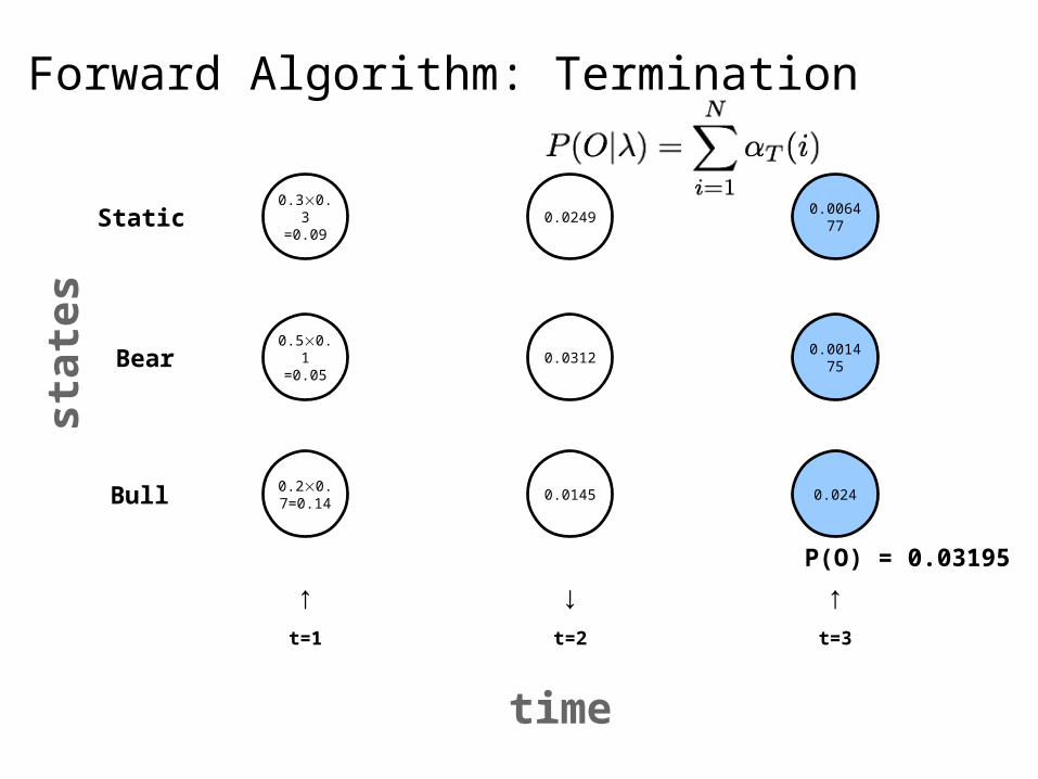
Forward Algorithm: Termination
time
↑ ↓ ↑t=1 t=2 t=3
0.20.7=0.14
0.50.1=0.05
0.30.3=0.09
0.0145
0.0312
0.0249
0.024
0.001475
0.006477
P(O) = 0.03195
Bear
Bull
Static
stat
es
HMM Problem #2: Decoding
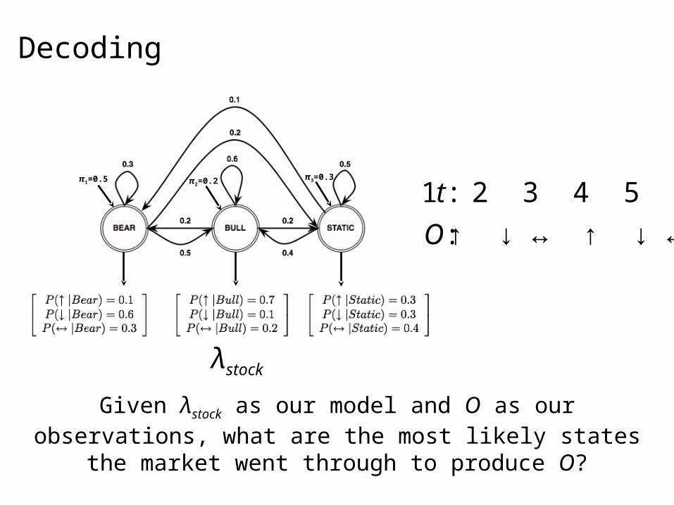
Decoding
Given λstock as our model and O as our observations, what are the most likely states the market went through to produce O?
1 2 3 4 5 6t:
↑ ↓ ↔ ↑ ↓ ↔O:
λstock
π1=0.5 π2=0.2 π3=0.3
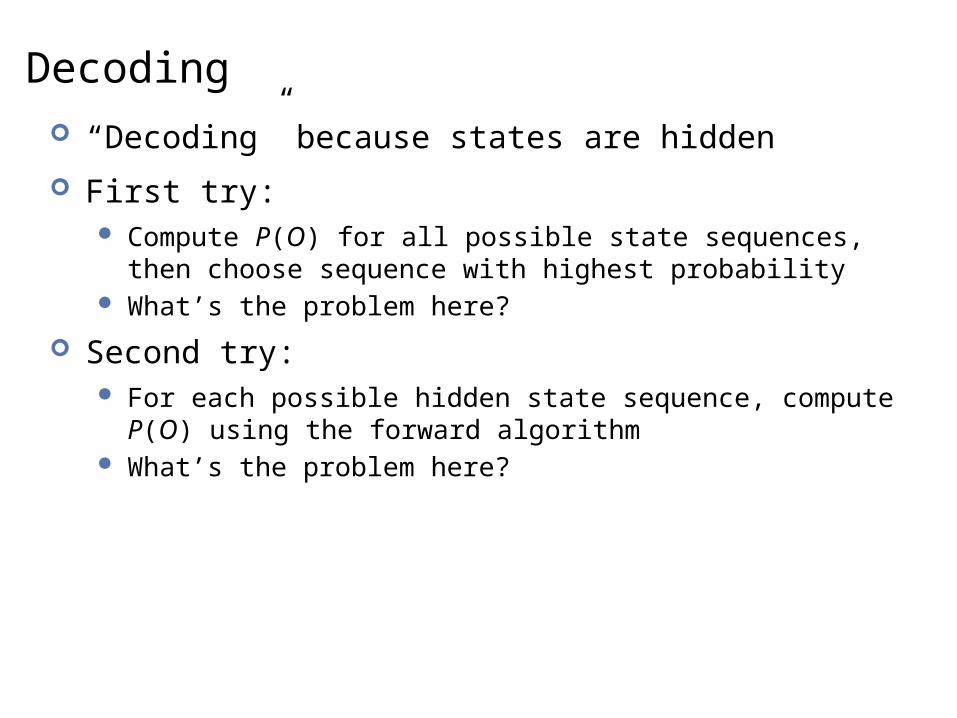
Decoding “Decoding” because states are hidden
First try: Compute P(O) for all possible state sequences, then choose
sequence with highest probability What’s the problem here?
Second try: For each possible hidden state sequence, compute P(O) using the
forward algorithm What’s the problem here?
Viterbi Algorithm “Decoding” = computing most likely state sequence
Another dynamic programming algorithm Efficient: polynomial vs. exponential (brute force)
Same idea as the forward algorithm Store intermediate computation results in a trellis Build new cells from existing cells
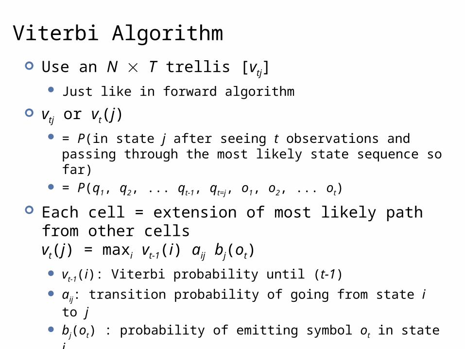
Viterbi Algorithm Use an N T trellis [vtj]
Just like in forward algorithm
vtj or vt(j) = P(in state j after seeing t observations and passing through the
most likely state sequence so far) = P(q1, q2, ... qt-1, qt=j, o1, o2, ... ot)
Each cell = extension of most likely path from other cellsvt(j) = maxi vt-1(i) aij bj(ot)
vt-1(i): Viterbi probability until (t-1)
aij: transition probability of going from state i to j
bj(ot) : probability of emitting symbol ot in state j
P = maxi vT(i)
Viterbi vs. Forward Maximization instead of summation over previous paths
This algorithm is still missing something! In forward algorithm, we only care about the probabilities What’s different here?
We need to store the most likely path (transition): Use “backpointers” to keep track of most likely transition At the end, follow the chain of backpointers to recover the most
likely state sequence
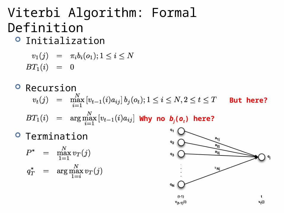
Viterbi Algorithm: Formal Definition Initialization
Recursion
Termination
Why no b() ?
Why no bj(ot) here?
But here?
Viterbi Algorithm
↑ ↓ ↑O =
find most likely state sequence given λstock
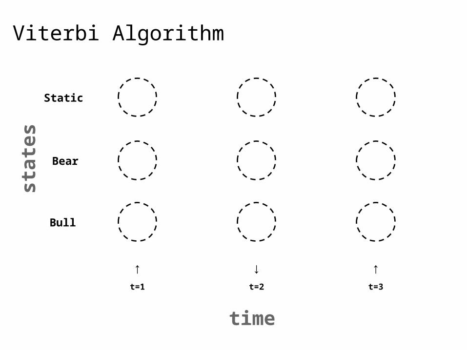
Viterbi Algorithm
time
↑ ↓ ↑t=1 t=2 t=3
Bear
Bull
Static
stat
es
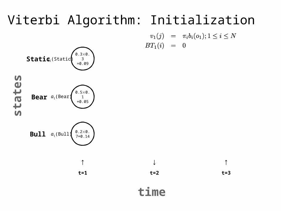
Viterbi Algorithm: Initialization
α1(Bull)
α1(Bear)
α1(Static)
time
↑ ↓ ↑t=1 t=2 t=3
0.20.7=0.14
0.50.1=0.05
0.30.3=0.09
Bear
Bull
Static
stat
es
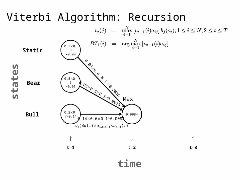
Viterbi Algorithm: Recursion
0.140.60.1=0.0084
0.050.50.1=0.0025
0.090.40.1 =0.0036
Max
α1(Bull)aBullBullbBull(↓)
time
↑ ↓ ↑t=1 t=2 t=3
0.20.7=0.14
0.50.1=0.05
0.30.3=0.09
0.0084
Bear
Bull
Static
stat
es
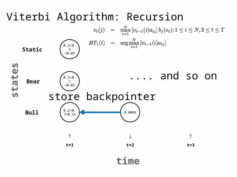
Viterbi Algorithm: Recursion
.... and so on
time
↑ ↓ ↑t=1 t=2 t=3
0.20.7=0.14
0.50.1=0.05
0.30.3=0.09
0.0084
Bear
Bull
Static
stat
es
store backpointer
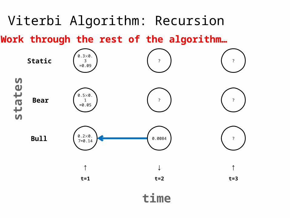
Viterbi Algorithm: Recursion
time
↑ ↓ ↑t=1 t=2 t=3
Bear
Bull
Static
stat
es
0.20.7=0.14
0.50.1=0.05
0.30.3=0.09
0.0084
?
?
?
?
?
Work through the rest of the algorithm…
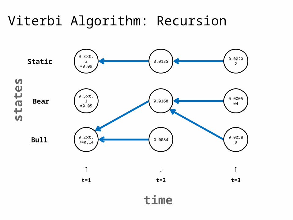
Viterbi Algorithm: Recursion
time
↑ ↓ ↑t=1 t=2 t=3
Bear
Bull
Static
stat
es
0.20.7=0.14
0.50.1=0.05
0.30.3=0.09
0.0084
0.0168
0.0135
0.00588
0.000504
0.00202
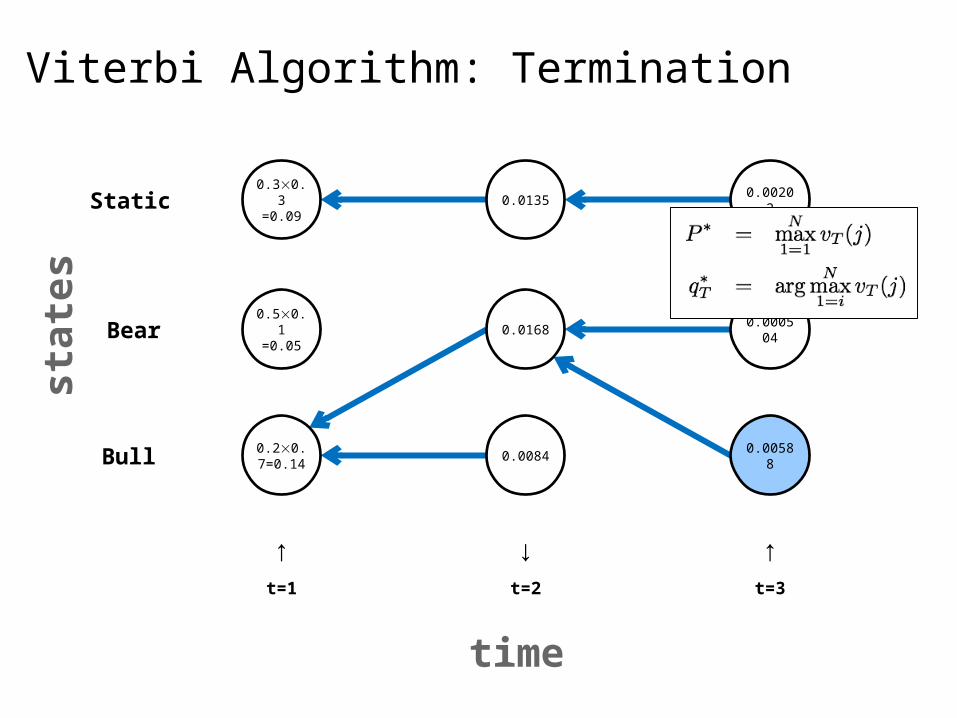
Viterbi Algorithm: Termination
time
↑ ↓ ↑t=1 t=2 t=3
Bear
Bull
Static
stat
es
0.20.7=0.14
0.50.1=0.05
0.30.3=0.09
0.0084
0.0168
0.0135
0.00588
0.000504
0.00202
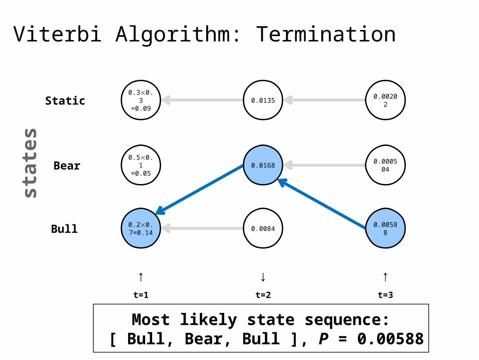
Viterbi Algorithm: Termination
time
↑ ↓ ↑t=1 t=2 t=3
Bear
Bull
Static
stat
es
0.20.7=0.14
0.50.1=0.05
0.30.3=0.09
0.0084
0.0168
0.0135
0.00588
0.000504
0.00202
Most likely state sequence: [ Bull, Bear, Bull ], P = 0.00588

POS Tagging with HMMs
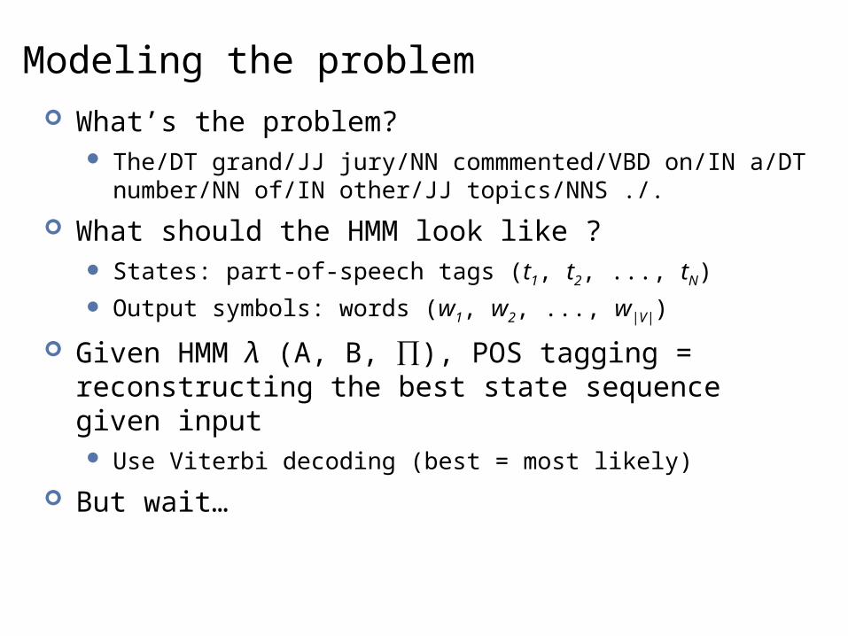
Modeling the problem What’s the problem?
The/DT grand/JJ jury/NN commmented/VBD on/IN a/DT number/NN of/IN other/JJ topics/NNS ./.
What should the HMM look like ? States: part-of-speech tags (t1, t2, ..., tN)
Output symbols: words (w1, w2, ..., w|V|)
Given HMM λ (A, B, ∏), POS tagging = reconstructing the best state sequence given input Use Viterbi decoding (best = most likely)
But wait…
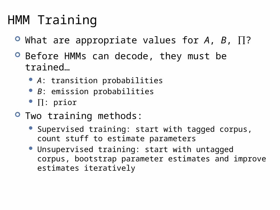
HMM Training What are appropriate values for A, B, ∏?
Before HMMs can decode, they must be trained… A: transition probabilities B: emission probabilities ∏: prior
Two training methods: Supervised training: start with tagged corpus, count stuff to
estimate parameters Unsupervised training: start with untagged corpus, bootstrap
parameter estimates and improve estimates iteratively
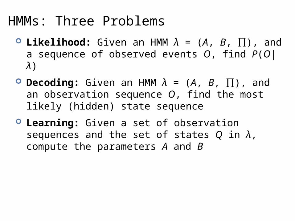
HMMs: Three Problems Likelihood: Given an HMM λ = (A, B, ∏), and a sequence
of observed events O, find P(O|λ)
Decoding: Given an HMM λ = (A, B, ∏), and an observation sequence O, find the most likely (hidden) state sequence
Learning: Given a set of observation sequences and the set of states Q in λ, compute the parameters A and B
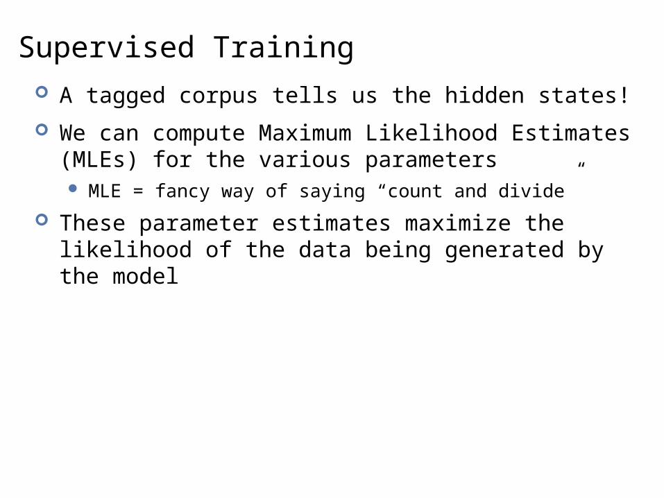
Supervised Training A tagged corpus tells us the hidden states!
We can compute Maximum Likelihood Estimates (MLEs) for the various parameters MLE = fancy way of saying “count and divide”
These parameter estimates maximize the likelihood of the data being generated by the model
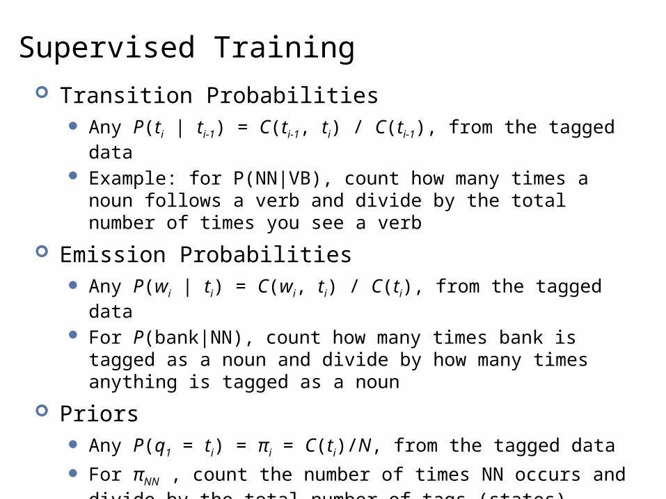
Supervised Training Transition Probabilities
Any P(ti | ti-1) = C(ti-1, ti) / C(ti-1), from the tagged data Example: for P(NN|VB), count how many times a noun follows a
verb and divide by the total number of times you see a verb
Emission Probabilities Any P(wi | ti) = C(wi, ti) / C(ti), from the tagged data For P(bank|NN), count how many times bank is tagged as a noun
and divide by how many times anything is tagged as a noun
Priors Any P(q1 = ti) = πi = C(ti)/N, from the tagged data
For πNN , count the number of times NN occurs and divide by the total number of tags (states)
A better way?
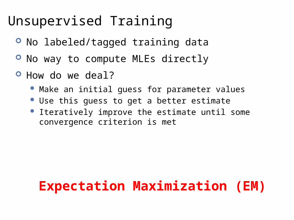
Unsupervised Training No labeled/tagged training data
No way to compute MLEs directly
How do we deal? Make an initial guess for parameter values Use this guess to get a better estimate Iteratively improve the estimate until some convergence criterion is
met
Expectation Maximization (EM)
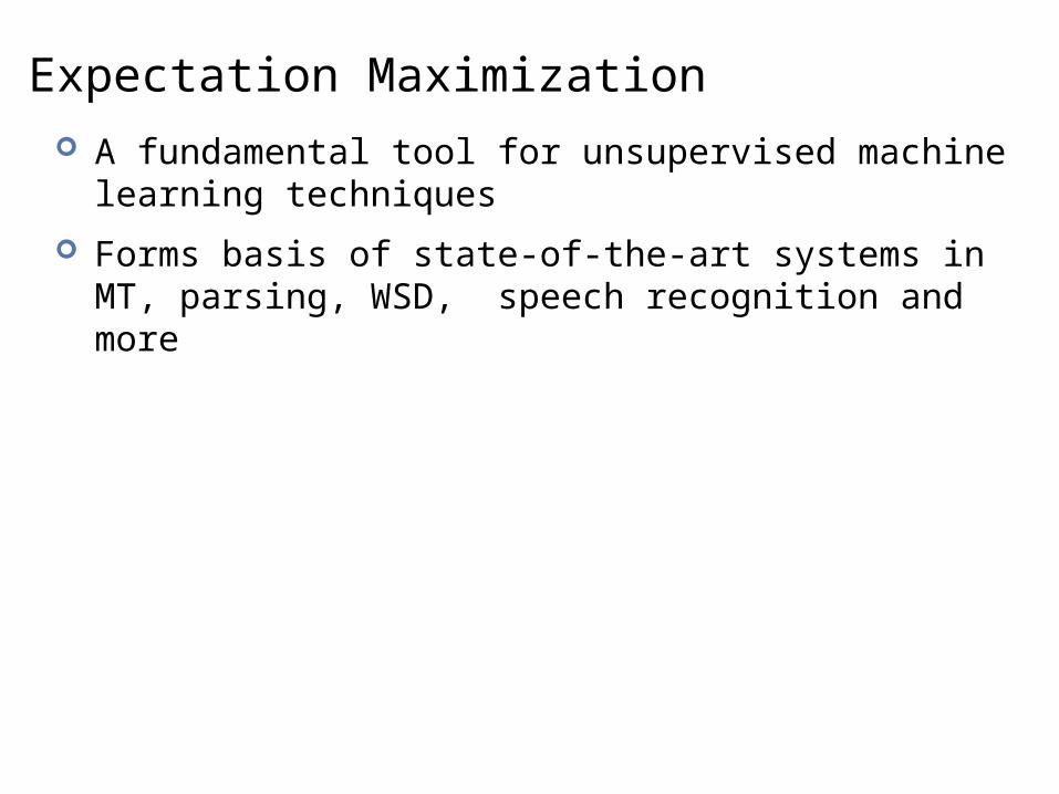
Expectation Maximization A fundamental tool for unsupervised machine learning
techniques
Forms basis of state-of-the-art systems in MT, parsing, WSD, speech recognition and more
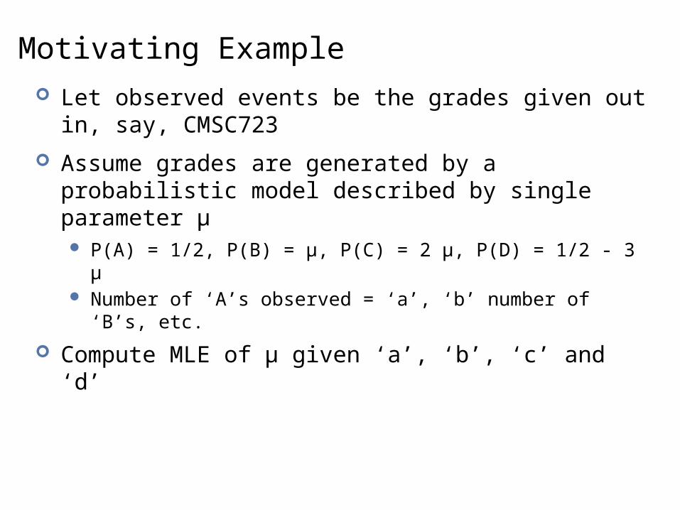
Motivating Example Let observed events be the grades given out in, say,
CMSC723
Assume grades are generated by a probabilistic model described by single parameter μ P(A) = 1/2, P(B) = μ, P(C) = 2 μ, P(D) = 1/2 - 3 μ Number of ‘A’s observed = ‘a’, ‘b’ number of ‘B’s, etc.
Compute MLE of μ given ‘a’, ‘b’, ‘c’ and ‘d’
Adapted from Andrew Moore’s Slideshttp://www.autonlab.org/tutorials/gmm.html
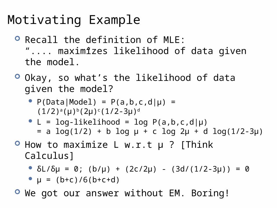
Motivating Example Recall the definition of MLE:
“.... maximizes likelihood of data given the model.”
Okay, so what’s the likelihood of data given the model? P(Data|Model) = P(a,b,c,d|μ) = (1/2)a(μ)b(2μ)c(1/2-3μ)d
L = log-likelihood = log P(a,b,c,d|μ)= a log(1/2) + b log μ + c log 2μ + d log(1/2-3μ)
How to maximize L w.r.t μ ? [Think Calculus] δL/δμ = 0; (b/μ) + (2c/2μ) - (3d/(1/2-3μ)) = 0 μ = (b+c)/6(b+c+d)
We got our answer without EM. Boring!
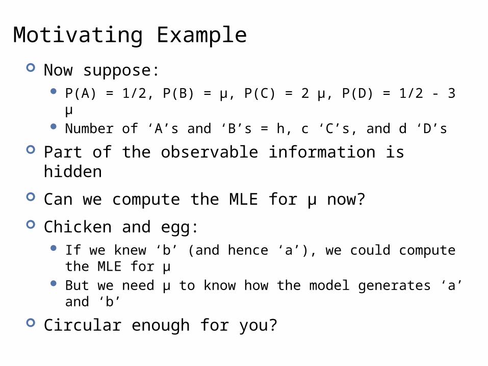
Motivating Example Now suppose:
P(A) = 1/2, P(B) = μ, P(C) = 2 μ, P(D) = 1/2 - 3 μ Number of ‘A’s and ‘B’s = h, c ‘C’s, and d ‘D’s
Part of the observable information is hidden
Can we compute the MLE for μ now?
Chicken and egg: If we knew ‘b’ (and hence ‘a’), we could compute the MLE for μ But we need μ to know how the model generates ‘a’ and ‘b’
Circular enough for you?
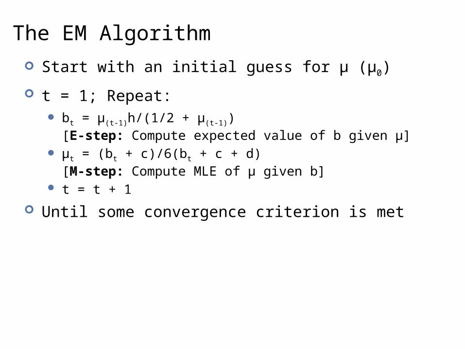
The EM Algorithm Start with an initial guess for μ (μ0)
t = 1; Repeat: bt = μ(t-1)h/(1/2 + μ(t-1))
[E-step: Compute expected value of b given μ] μt = (bt + c)/6(bt + c + d)
[M-step: Compute MLE of μ given b] t = t + 1
Until some convergence criterion is met
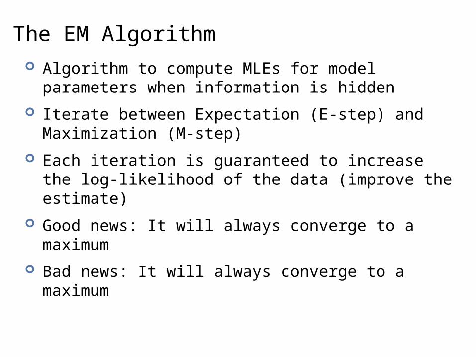
The EM Algorithm Algorithm to compute MLEs for model parameters when
information is hidden
Iterate between Expectation (E-step) and Maximization (M-step)
Each iteration is guaranteed to increase the log-likelihood of the data (improve the estimate)
Good news: It will always converge to a maximum
Bad news: It will always converge to a maximum
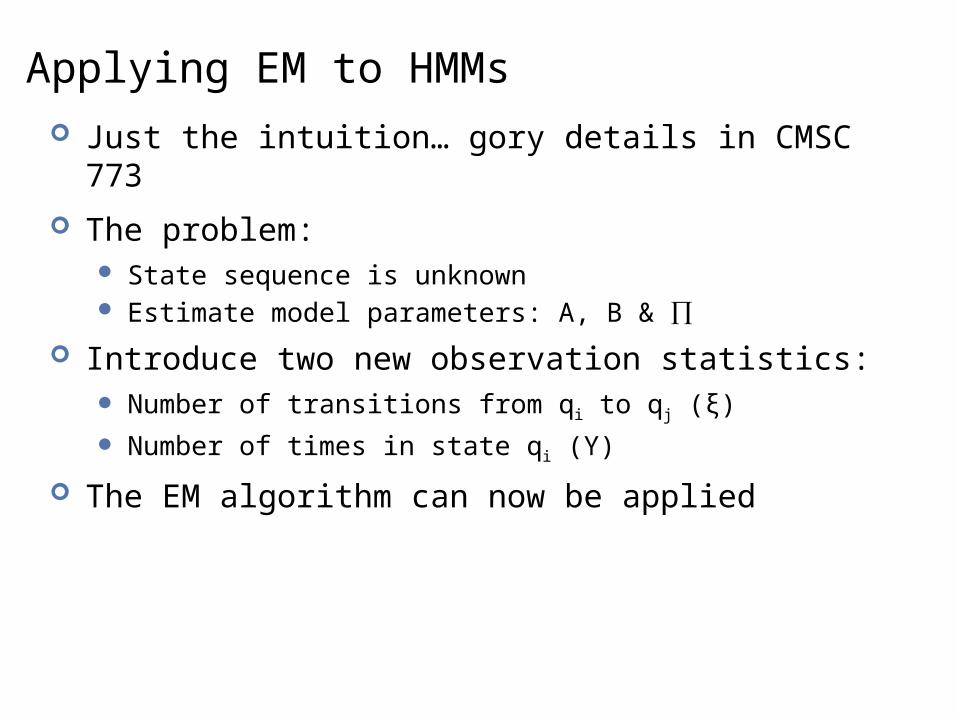
Applying EM to HMMs Just the intuition… gory details in CMSC 773
The problem: State sequence is unknown Estimate model parameters: A, B & ∏
Introduce two new observation statistics: Number of transitions from qi to qj (ξ)
Number of times in state qi (ϒ)
The EM algorithm can now be applied
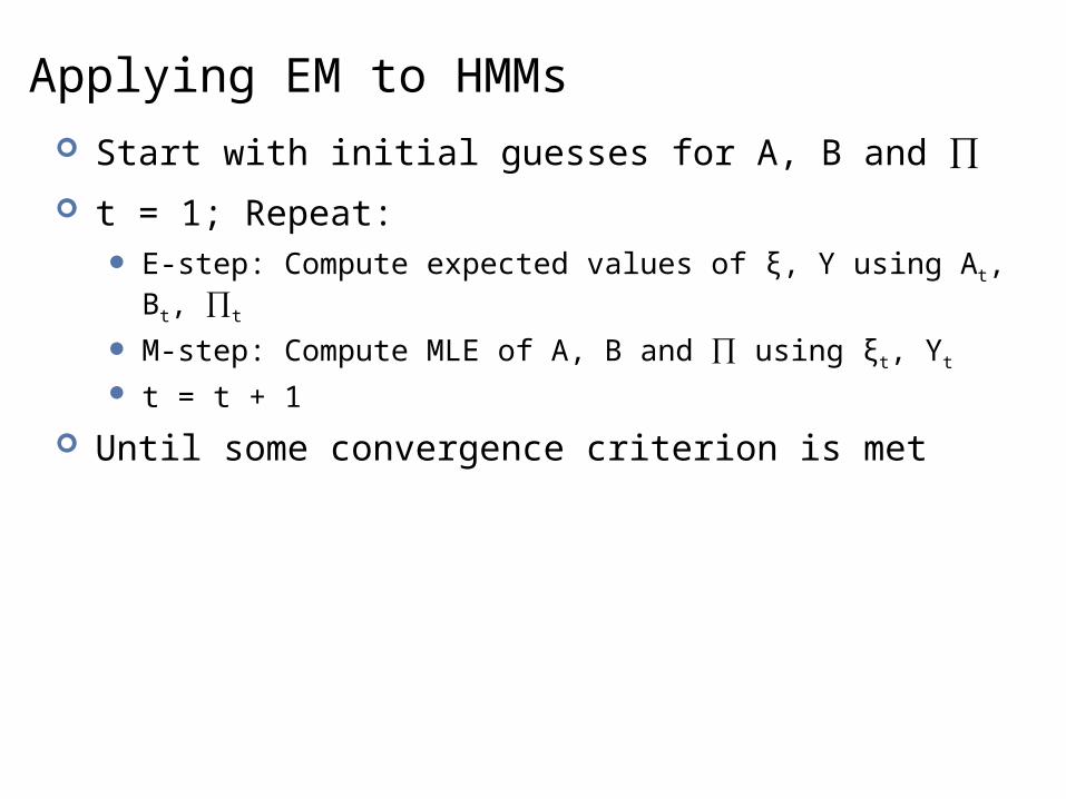
Applying EM to HMMs Start with initial guesses for A, B and ∏
t = 1; Repeat: E-step: Compute expected values of ξ, ϒ using At, Bt, ∏t
M-step: Compute MLE of A, B and ∏ using ξt, ϒt
t = t + 1
Until some convergence criterion is met
What we covered today… The great leap forward in NLP
Hidden Markov models (HMMs) Forward algorithm Viterbi decoding Supervised training Unsupervised training teaser
HMMs for POS tagging