Hidden flavor symmetries of SO(10) GUT

Borut Bajca,1 and Alexei Yu. Smirnovb,c,2

a J. Stefan Institute, 1000 Ljubljana, Sloveniab Max-Planck-Institut fur Kernphysik, Saupfercheckweg 1, D-69117 Heidelberg, Germanyc International Centre for Theoretical Physics, Strada Costiera 11, I-34100 Trieste, Italy

Abstract

The Yukawa interactions of the SO(10) GUT with fermions in 16-plets (as well aswith singlets) have certain intrinsic (“built-in”) symmetries which do not depend onthe model parameters. Thus, the symmetric Yukawa interactions of the 10 and 126dimensional Higgses have intrinsic discrete Z2 × Z2 symmetries, while the antisym-metric Yukawa interactions of the 120 dimensional Higgs have a continuous SU(2)symmetry. The couplings of SO(10) singlet fermions with fermionic 16-plets haveU(1)3 symmetry. We consider a possibility that some elements of these intrinsic sym-metries are the residual symmetries, which originate from the (spontaneous) breakingof a larger symmetry group Gf . Such an embedding leads to the determination ofcertain elements of the relative mixing matrix U between the matrices of Yukawacouplings Y10, Y126, Y120, and consequently, to restrictions of masses and mixingsof quarks and leptons. We explore the consequences of such embedding using thesymmetry group conditions. We show how unitarity emerges from group propertiesand obtain the conditions it imposes on the parameters of embedding. We find thatin some cases the predicted values of elements of U are compatible with the existingdata fits. In the supersymmetric version of SO(10) such results are renormalizationgroup invariant.

1borut.bajc@ijs.si2smirnov@mpi-hd.mpg.de

1

arX

iv:1

605.

0795

5v2

[he

p-ph

] 2

1 Ju

n 20

16

Contents

1 Introduction 2

2 Intrinsic flavor symmetries of SO(10) 42.1 Relative mixing matrices . . . . . . . . . . . . . . . . . . . . . . . . . . . . 42.2 Intrinsic symmetries . . . . . . . . . . . . . . . . . . . . . . . . . . . . . . 4

3 Embedding intrinsic symmetries 63.1 Embedding of two transformations . . . . . . . . . . . . . . . . . . . . . . 63.2 Embedding of bigger residual symmetries and Unitarity . . . . . . . . . . . 93.3 The case with 120H coupling . . . . . . . . . . . . . . . . . . . . . . . . . . 11

4 Confronting relations with data 154.1 The case of Y10 + Y126 . . . . . . . . . . . . . . . . . . . . . . . . . . . . . . 164.2 Relative mixing between Y10 and Y120 . . . . . . . . . . . . . . . . . . . . . 164.3 RG invariance of the residual symmetry . . . . . . . . . . . . . . . . . . . . 17

5 SO(10) model with hidden sector 18

6 Intrinsic symmetries and relative mixing matrix 19

7 Summary and Conclusion 21

A Comparison with the approach in [13] 23

1 Introduction

In spite of various open questions, Grand Unification [1, 2] is still one of the most appealingand motivated scenarios of physics beyond the standard model. The models based onSO(10) gauge symmetry [3, 4, 5] are of special interest since they embed all known fermionsof a given generation and the right handed neutrinos in a single multiplet 3. One of the openquestions is to understand the flavor structures - observed fermion masses and mixings,which SO(10) unification alone can not fully address4. Moreover, embedding of all thefermions in a single multiplet looks at odds with different mass hierarchies and mixings,and in particular with the strong difference of mixing patterns of quarks and leptons.

The Yukawa sector of the renormalizable5 version of SO(10) GUT [7] with three gener-ations of matter fields in 16F is given by

LY ukawa = 16TF(Y1010H + Y126126H + Y120120H

)16F , (1.1)

where the 3× 3 matrices of Yukawa couplings, Y10, Y126 and Y120 correspond to Higgses in10H , 126H and 120H . The masses and mixings of the Standard Model (SM) fermions are

3We consider here theories with no extra vector-like matter which could mix with SM fermions. This isthe case of the majority of available models, but may not be the case if SO(10) is coming from E6.

4 Partially it sometimes can: for example, b − τ unification can be related to the large atmosphericmixing angle in models with dominant type II seesaw [6].

5To realize eventually our scenario these Yukawa couplings should be VEVs of fields which transformnon-trivially under some flavor group Gf - so they will be non-renormalizable, or we should ascribe chargesto the Higgs multiplets.

2

determined by these Yukawa couplings Ya, the Clebsch-Gordan coefficients and the VEV’sof the light Higgs(es). So, to make predictions for the masses and mixing one needs, inturn, to determine the matrices Ya (a = 10, 126, 120).

There are various attempts to impose a flavor symmetry on the Yukawa interaction (1.1)to restrict the mass and mixing parameters, see for example [8] for continuous symmetries,[9, 10, 11] for discrete symmetries, and [12] for reviews. In most cases flavor symmetriesappear as horizontal symmetries - which are independent of the vertical gauge symmetrySO(10).

Two interesting ideas have been discussed recently which employ an interplay betweenthe GUT symmetry and flavor symmetries and may lead to deep relation between them.

1. Existence of “natural” (“built-in”) or intrinsic flavor symmetries [13]. Examples areknown from the past that some approximate flavor symmetries can arise from the “vertical”gauge symmetries. One of these is the antisymmetry of the Yukawa couplings of the leptondoublets with charged scalar singlet. The neutrino mass matrix generated at 1-loop (Zeemodel [14]) has specific flavor structure with zero diagonal terms.

It is well known that SO(10) have such flavor symmetries. The three terms in (1.1) havesymmetries dictated by “vertical” SO(10): symmetricity of the Yukawa coupling matricesof the 10-plet and 126-plet of Higgses and antisymmetricity of the Yukawa coupling matrixof the 120-dimensional Higgs multiplets:

Y T10,126 = Y10,126 , Y T

120 = −Y120. (1.2)

The first equality (symmetricity) implies a Z2 × Z2 symmetry [13]. For the antisymmetricmatrix (second equality) the symmetry (Z2) has been taken in [13] (or (Z2)

2 if negativedeterminants are allowed).

2. Identification of the natural symmetries with residuals of the flavor symmetry [13].This idea is taken from the residual symmetry approach developed to explain the leptonmixing. It states that some or all elements of the natural symmetries of SO(10) are actu-ally the residual symmetries which originate from the breaking of a bigger flavor symmetrygroup Gf [15, 16, 17, 18, 19]. In [13] it was proposed to embed the residual (Z2)

n, whichare reflection symmetries, into the minimal group with a three-dimensional representation.This leads to the Coxeter group and finite Coxeter groups of rank 3 and 4 have been con-sidered. The embedding of natural symmetries into the flavor (Coxeter) group imposesrestrictions on the structure of Ya and consequently on the mass matrices, which reducesthe number of free parameters.

In this paper we further elaborate on realizations of these ideas, although from a differentpoint of view. While the intrinsic symmetries of Y10 and Y126 are Z2 × Z2, as in [13], wefind that Y120 has a bigger symmetry - SU(2). Furthermore, we consider the situation whenSO(10) singlet fermions are present. From the embedding of intrinsic symmetries and withthe use of symmetry group relations [20, 21] we obtain predictions for the elements of therelative mixing matrix Ua−b (a, b = 10, 126, 120) between the Yukawa couplings Ya and Yb(Ua−b connects the bases in which matrices Ya and Yb are diagonal). These unitary matricesUa−b are basis independent, in contrast to the matrices Ya and Yb themselves. We re-derivethese relations and elaborate on the unitarity condition, showing that it follows from groupproperties. We confront the predictions with the results of some available data fits.

3

The paper is organized as follows. In sect. 2 we explore the intrinsic symmetries of theSO(10) Yukawa couplings. In sect. 3 we identify (part of) the intrinsic symmetries withthe residual symmetries and consider their embedding into a bigger flavor group. Usingthe symmetry group relations we obtain predictions for different elements of the relativematrix U . We elaborate on the unitarity condition which gives additional bounds on theparameters of embedding. We consider separately the embeddings of the 120H couplings.This case has not been covered in [13] and we develop various methods to deal with it.In sect. 4 we confront our predictions for the mixing matrix elements with the resultsobtained from existing fits of data. In sect. 5 we consider symmetries in the presence of theSO(10) fermionic singlets. In sect. 6 we summarize the concept of intrinsic symmetry andthe relative mixing matrix. Summary of our results and conclusion are presented in sect.7. We compare our approach with that in [13] in Appendix A, suggesting an equivalence.

2 Intrinsic flavor symmetries of SO(10)

2.1 Relative mixing matrices

The matrices of Yukawa couplings are basis dependent. It is their eigenvalues and therelative mixings which have physical meaning. The relative mixing matrices, which are themain object of this paper, are defined in the following way. The symmetric matrices Y10and Y126 can be diagonalized with the unitary transformation matrices U10 and U126 as

Y10 = U∗10Yd10U

†10, (2.1)

andY126 = U∗126Y

d126U

†126. (2.2)

Mixing is generated if the matrices Ya can not be diagonalized simultaneously. The relativemixing matrix U10−126 is given by

U10−126 = U †10U126. (2.3)

This matrix, in contrast to matrices of Yukawa couplings, does not depend on basis andhas immediate physical meaning. In a sense, it is the analogy of the PMNS (or CKM)matrix which connects bases of mass states of neutrinos and charged leptons. Similarly wecan introduce the relative mixing matrices for other Yukawa coupling matrices as

Ua−b = U †aUb, (2.4)

e.g., U10−120, U120−126, etc.The symmetry formalism we present below (symmetry group relations) will determine

elements of the relative matrices immediately without consideration of the symmetric ma-trices Ya and their diagonalization.

2.2 Intrinsic symmetries

All the terms of the Lagrangian (1.1) have the same fermionic structure, being the Majoranatype bilinears of 16F . This by itself implies certain symmetry. For definiteness let usconsider the basis of three 16F plets in which the Yukawa coupling of the 10-plet is diagonal:

Y10 = Y d10. (2.5)

4

In this basis the Yukawa matrix of 126H (being in general non-diagonal) can be diagonalizedby the unitary matrix U126 as in (2.2). In this basis U126 gives immediately the relativemixing matrix U10−126 = U126. It is straightforward to check that the symmetric matricesY d10 and Y126 are invariant with respect to transformations

Sdj Yd10S

dj = Y d

10 , j = 1, 2, 3, (2.6)

(S126)Ti Y126 (S126)i = Y126 , i = 1, 2, 3, (2.7)

where(S126)i = U126S

di U†126, (2.8)

and the diagonal transformations equal

Sd1 = diag(1, − 1, − 1), Sd3 = diag(−1, − 1, 1), (2.9)

Sd2 = Sd1Sd3 . (We use generators with Det[Si] = +1, so that they can form a subgroup of

SU(3)).The transformations (2.9) can be written as(

Sdj)ab

= 2δajδbj − δab, (2.10)

and a, b = 1, 2, 3. All these transformations (reflections) obey

(Sj)2 = (Sdj )2 = I. (2.11)

Thus, Y d10 is invariant under the group of transformations G10 = Z2 × Z2 consisting of

elementsG10 = {1, Sd1 , Sd2 , Sd3}. (2.12)

The matrix Y126 is invariant under another, G126 = Z2 × Z2 group consisting of U− trans-formed elements

G126 = U126{1, Sd1 , Sd2 , Sd3}U†126, (2.13)

where U126 is defined in (2.2).This intrinsic symmetry is always present independently of parameters of the model due

to the symmetric Yukawa matrices Y10 and Y126 [13] which follow from SO(10) symmetry.

In the case of antisymmetric Yukawa interactions of 120H the situation is different. Theantisymmetric matrix Y120 can be put in the canonical form

Y c120 =

0 0 00 0 x0 −x 0

(2.14)

by the unitary transformation U120 as

Y120 = U∗120Yc120U

†120. (2.15)

The matrix (2.14) is invariant with respect to SU(2)×U(1) transformations

gTY c120g = Y c

120. (2.16)

5

Again we will bound ourselves to group elements with Det(g) = 1, keeping in mind possibleembedding into SU(3). Then there is no U(1), and therefore

G120 = SU(2). (2.17)

The SU(2) transformation element g can be written as

g(~φ) =

(1 0

0 exp(i~φ~τ))

=

(1 0

0 cosφ+ i~φ~τφ

sinφ

)(2.18)

with ~φ = (φ1, φ2, φ3), φ ≡ |~φ| ∈ [0, π] and ~τ being the Pauli matrices.Although the symmetry of the Yukawa matrix connected to the 120-plet is continuous,

we should use only its discrete subgroup to be a part of Gf , since Gf itself has been assumed

to be discrete. This means that the angle ~φ should take discrete values such that(g(~φ)

)p= I (2.19)

for some integer p. The angle can be parametrized as

~φ = 2πn

pφ , n = 1, . . . , p− 1, (2.20)

where φ ≡ ~φ/|~φ| (so that φ2 = 1). In this paper we will consider a Zp subgroup of theAbelian U(1) ⊂ SU(2). So, the elements gφ, g

2φ, . . . , g

p−1φ can be written as

gnφ =

(1 0

0 exp(i2π(~τ φ)n/p

)). (2.21)

More on intrinsic symmetries and the mixing matrices can be found in Appendix 6.Intrinsic symmetries for the SO(10) singlets are discussed in sect. 5.

We assume throughout this paper that the Higgs multiplets are uncharged with respectto Gf . Introduction of Higgs charges can lead to suppression of some Yukawa couplingsbut does not produce the flavor structure of individual interactions.

3 Embedding intrinsic symmetries

Following [13] we assume that the intrinsic symmetries formulated in the previous sectionare actually residual

which result from the breaking of a larger (flavor) symmetry group Gf . In other words,some of the symmetries G10 and G126 or/and G120 are embedded into Gf . In the followingwe will derive various constraints on the relative mixing matrix U between two Yukawamatrices.

3.1 Embedding of two transformations

We recall the symmetry group relation formalism [20, 21] adopted to our SO(10) case. Theformalism allows to determine (basis independent) elements of the relative mixing matriximmediately without explicit construction of Yukawa matrices. Let us first consider the

6

Yukawa couplings of 10H and 126H . Suppose the covering group Gf contain Sdj ∈ G10 andSi ∈ G126. Since Si, S

dj ∈ Gf , the product SiS

dj should also belong to Gf : SiS

dj ∈ Gf . Then

the condition of finiteness of Gf requires that a positive integer pji exists such that(SiS

dj

)pji= I. (3.1)

This is the symmetry group relation [20, 21] which we will use in our further study. InsertingSi = USdi U

†6 into (3.1) we obtain [20, 21]

(Wij)pji = I, (3.2)

whereWij ≡ USdi U

†Sdj . (3.3)

Furthermore, we will impose the condition

Det[Wij] = 1 (3.4)

keeping in mind a possible embedding into SU(3). We will comment on the case of negativedeterminant later.

The simplest possibility is the residual symmetries Z(10)2 ×Z(126)

2 , that is Z2 for Y10 andanother Z2 for Y126. In this case the flavor symmetry group Gf is always a finite von Dyckgroup (2, 2, p), since

1

2+

1

2+

1

p> 1 (3.5)

for any positive integer p.Let us elaborate on the constraint (3.1) further, providing derivation of the relations

slightly different to that in [20, 21]. According to the Schur decomposition we can presentWij in the form

Wij = VW upperij V †, (3.6)

where V is a unitary matrix and W upperij is an upper triangular matrix, the so called Schur

form of Wij. Since unitary transformations do not change the trace, we have from (3.6)

Tr[Wij] = Tr[W upperij ]. (3.7)

The diagonal elements of W upperij are the (in general complex) eigenvalues of Wij which we

denote by λα. Therefore,Tr[W upper

ij ] = apji , (3.8)

whereapji ≡

∑α

λα. (3.9)

Inserting (3.6) into condition (3.2) and using unitarity of V we obtain

(W upperij )pji = diag(λ

pji1 , λ

pji2 , λ

pji3 ) = I (3.10)

the off-diagonal elements in the LH side should be zero to match with the RH side).Consequently, the eigenvalues of W equal the pji - roots of unity:

λα = pji√

1. (3.11)

6In this and the next section U ≡ U10−126.

7

Finally, Eq. (3.8) givesTr[Wij] = apji , (3.12)

where apji is defined in (3.9).The pji−roots of unity can be parametrized as

λ = exp (i2πkji/pji) , kji = 1, . . . , pji − 1. (3.13)

For p ≥ 3 the number of p-roots is larger than 3, and therefore there is an ambiguity inselecting the three values to compose apji . However, not all combinations can be used, andcertain restrictions will be discussed in the following.

Restriction on apji arises from the following consideration. The eigenvalues λα satisfythe characteristic polynomial equation Wij:

Det (λI−Wij) = λ3 − apjiλ2 + a∗pjiλ− 1 = 0, (3.14)

where apji is defined in (3.9)7. Consider the conjugate of Eq. (3.14). Using the expression

for (3.3) and taking into account that(Sdi)2

= I we obtain

W †ij = SdjWijS

dj . (3.16)

This in turn gives for the LHS of the conjugate equation

Det(λ∗I−W †

ij

)= Det

(λ∗I− SdjWijS

dj

)= Det

[Sdj (λ∗I−Wij)S

dj

]= Det (λ∗I−Wij) .

(3.17)Therefore the set of eigenvalues {λα} coincides with the set {λ∗α} [22]. Then it is easy tocheck that this is possible only if one of λα equals unit, e.g. λ1 = 1, and two others areconjugate of each other: λ3 = λ∗2 ≡ λ. Thus,

apji = a∗pji = 1 + λ+ λ∗ = 1 + 2Reλ, (3.18)

or explicitly,apji = 1 + 2 cos (2πkji/pji) = −1 + 4 cos2 (πkji/pji). (3.19)

On the other hand, from definitions of Sj (2.10) and (3.3), we find explicitly

Tr (Wij) = 4 |Uji|2 − 1 (3.20)

or using (3.12) (see also [23])

|Uji|2 =1

4

(1− apji

). (3.21)

Notice that the trace (3.20) is real, and therefore apji = a∗pji , leading to the form (3.18).Finally, inserting apji from (3.19) we obtain

|Uji| = |cos (πkji/pji)| . (3.22)

7 This can be obtained noticing that

Det (λI−Wij) = (λ− λ1)(λ− λ2)(λ− λ3), (3.15)

|λi|2 = 1 and Det(Wij) ≡ λ1λ2λ3 = 1.

8

Similar expression has been obtained before in [24] in the Dihedral group model for theCabibbo angle (Vus). The expression appears also in [25].

Thus, we obtain thus a relation for a single element of the matrix U , as the consequenceof the Z

(10)2 × Z(126)

2 residual symmetry. The element |Uji| is determined by two discreteparameters – arbitrary integers pji and kji = 0, . . . , pji−1. The expression does not dependon the selected Si. The elements Si and Sj just fix the ij− element of the matrix U , butnot its value, the value is determined by pji and kji.

Allowing also Det(Wij) = −1 we generalize (2.12) into

(Z2 × Z2)10 → {1, Sd1 , S

d2 , S

d3} ∪ {−1,−Sd1 ,−Sd2 ,−Sd3}, (3.23)

while in (3.3) Sdi (and/or Sdj ) can be replaced by −Sdi (and/or −Sdj ). A difference fromthe previous case comes only if in Wij the two diagonal group elements have opposite signsof determinants. In this case we have Det(Wij) = λ1λ2λ3 = −1 and since now one ofthe eigenvalues needs to be λ1 = −18, we obtain that λ2λ3 = 1 or λ2 = λ∗3 ≡ λ. Thenapji = −1 + λ+ λ∗ = −1 + 2Re(λ), and consequently,

|Uji| = |sin (πkji/pji)| , (3.25)

(as compared with (3.22)).

3.2 Embedding of bigger residual symmetries and Unitarity

Following the derivations in [22, 26] we summarize here the embedding of bigger residualsymmetries, when we take Z2 × Z2 from one of the interactions (10H or 126H) and one Z2

from the other interaction. Now there are three generating elements: for Z(10)2 ×Z(10)

2 ×Z(126)2

the matrix Y10 is invariant under Sdj and Sdk (j 6= k), whereas Y126 – under Si. Consequently,we have two symmetry group conditions:

(USdi U†Sdj )pji = I, (USdi U

†Sdk)pki = I (3.26)

which determine two elements of the matrix U from the same column i: |Uji| and |Uki|.Repeating the same procedure of the previous section we obtain

|Uji| = |cos (πkji/pji)| , |Uki| = |cos (πkki/pki)| . (3.27)

The second possibility is Z(10)2 ×Z(126)

2 ×Z(126)2 with one generating element for Y10 and

two for Y126. This gives also two symmetry group conditions but for two elements in thesame row of U . This is enough to determine the whole row (or column in the first case)from unitarity. Possible values of matrix elements for this case have been classified in wholegenerality [22, 26].

Using the complete symmetry Z(10)2 × Z(10)

2 × Z(126)2 × Z(126)

2 one can fix 4 elements ofU , and consequently, due to unitarity, the whole matrix U . This matrix is necessarily ofthe type classified in [22, 26].

8 The eigenvalues λ1,2,3 of Wij satisfy (|λα|2 = 1)

0 = Det (λI−Wij) = λ3 − (λ1 + λ2 + λ3)λ2 + (λ1λ2 + λ2λ3 + λ3λ1)λ− λ1λ2λ3= λ3 − apjiλ2 + Det (Wij) a

∗pjiλ−Det (Wij) . (3.24)

If a∗pji = apji , one eigenvalue is equal to Det(Wij).

9

Notice that values of the elements of the relative matrix U have been obtained usingdifferent group elements Sj (for fixed Si) essentially independently. They were determinedby the independent parameters pj, kj. However, there are relations between the groupelements Sj which, as we will see, lead to relations between parameters pj, kj, which areequivalent to relations required by unitarity of the matrix U .

According to (3.22) |Uji| ≤ 1 for any pair of values of k and p. For two elements in thesame line or column unitarity requires

cos2 (πk1/p1) + cos2 (πk2/p2) ≤ 1 (3.28)

and it is not fulfilled automatically. (In this section we omit the second index of k and p,which is the same for both. Keeping in mind that both are from the same line or the samecolumn.) Furthermore, the inequality (3.28) can not be satisfied for arbitrary ki and pi, andtherefore gives certain bounds on these parameters. This, in turn, affects the embedding(covering group). In what follows we will consider such restrictions on parameters k and pthat follow from relations between the group elements.

The elements of Z2 × Z2 group in 3 dimensional representation (2.9) or (2.10) satisfythe following equalities

3∑i=1

Sdi = −I, (3.29)

andTr (Si) = −1, i = 1, 2, 3. (3.30)

Let us find the corresponding relations between the parameters pi and ki. Summation overthe index i of the traces Tr[Wij], where Wij is given in eq. (3.3), gives

∑i

Tr[Wij] = Tr

[∑i

Wij

]= Tr

[U

(∑i

Sdi

)U †Sdj

]. (3.31)

The last expression in this formula together with equalities (3.29) and (3.30) gives−Tr[Sdj ] =1. Therefore

∑i Tr[Wij] = 1 and according to (3.12) we find

ap1 + ap2 + ap3 = 1. (3.32)

Finally, insertion of expressions for api in eq. (3.19) leads to

cos2 (πk1/p1) + cos2 (πk2/p2) + cos2 (πk3/p3) = 1. (3.33)

This coincides with the unitarity condition: Eq. (3.33) is nothing but∑

i |Uij|2 = 1, wherethe elements are expressed via cosines (3.22). So, the unitarity condition is encoded in therelation (3.29) which is equivalent to the unitarity. Thus, the unitarity condition whichimposes relations between pj and kj can be obtained automatically from properties of thegroup elements.

The condition is highly non-trivial since it should be satisfied for integer values of piand ki. It can be fulfilled for specific choices of (k1/p1, k2/p2, k3/p3). There are just fewcases which can satisfy (3.33). Some of these constraints have been found in [27, 28] from

10

specific assumptions on Gf . In general, it has been shown [22, 26] (see also [25]) that theonly possibilities are

{ci} ≡ (c1, c2, c3) =

(1√2,

1

2,

1

2

), (3.34)

where

ci ≡ cos

(πkipi

), i = 1, 2, 3. (3.35)

The values in (3.34) correspond to

(k1/p1, k2/p2, k3/p3) =

(1

4,

1

3,

1

3

). (3.36)

Another solution,

{ci} =

(1

2,φ

2,

1

2φ

), (3.37)

where

φ =

√5 + 1

2(3.38)

is the golden ratio. In this case

(k1/p1, k2/p2, k3/p3) =

(1

3,

1

5,

2

5

)(3.39)

Finally,{ci} = (cosα, sinα, 0) (3.40)

withα = πk0/p0 , 1 ≤ k0 ≤ p0/2 , k0 ∈ Z. (3.41)

They correspond to

(k1/p1, k2/p2, k3/p3) =

(k0p0,

1

2− k0p0,

1

2

). (3.42)

For instance for k0/p0 = 1/2 we obtain ci = (0, 1, 0), for k0/p0 = 1/3: ci = (1/2,√

3/2, 0),for k0/p0 = 1/4: ci = (1/

√2, 1/√

2, 0), etc.

3.3 The case with 120H coupling

The symmetry transformation of Y120 is given by the elements gnφ of a discrete subgroupZp of U(1) ⊂ SU(2) (2.21). Since g2φ 6= I for p > 2, the embedding symmetry group is nota Coxeter group, and so this analysis goes beyond the assumptions of [13]. If we assumethat the element gφ from the Zp intrinsic symmetry of Y120 and the element Sdj from theZ2 intrinsic symmetry of Y10 (or Y126) are residual symmetries, from the definition of agroup this is true also for all gnφ , n = 1 . . . , p− 1. Therefore, the symmetry group relations

now contain the products of UgnφU†9 - any of the symmetry elements of Y120, and Sdj which

belongs to the symmetry of Y d10 (or Y d

126):[W njφ

]p= I , W n

jφ = UgnφU†Sdj . (3.43)

9In this section U ≡ U10−120 (or U ≡ U126−120).

11

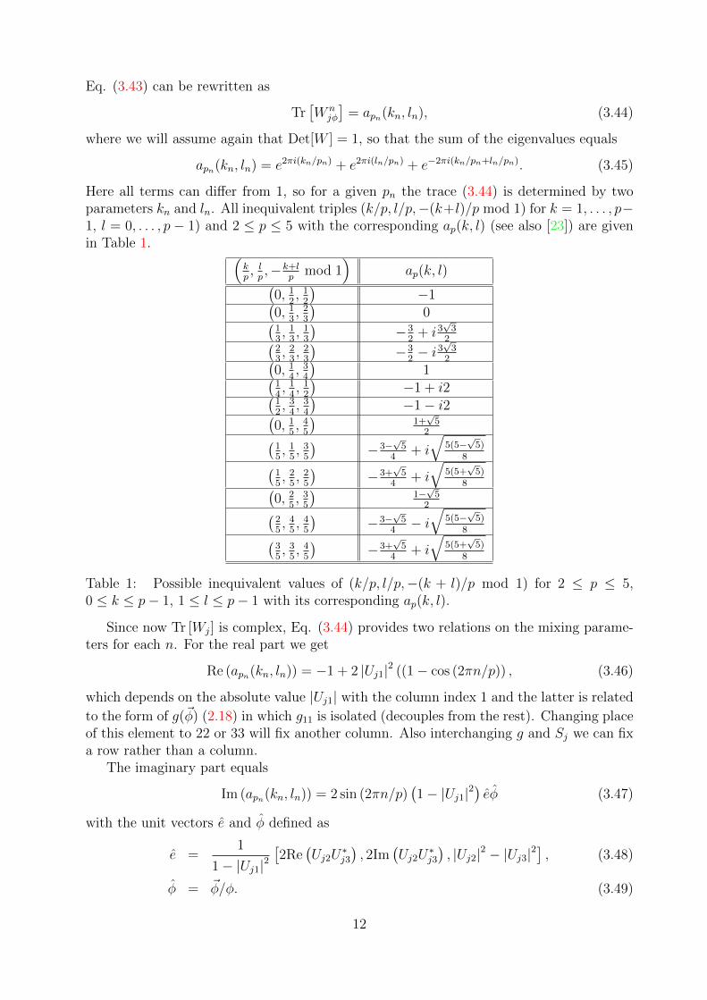
Eq. (3.43) can be rewritten as

Tr[W njφ

]= apn(kn, ln), (3.44)

where we will assume again that Det[W ] = 1, so that the sum of the eigenvalues equals

apn(kn, ln) = e2πi(kn/pn) + e2πi(ln/pn) + e−2πi(kn/pn+ln/pn). (3.45)

Here all terms can differ from 1, so for a given pn the trace (3.44) is determined by twoparameters kn and ln. All inequivalent triples (k/p, l/p,−(k+l)/p mod 1) for k = 1, . . . , p−1, l = 0, . . . , p− 1) and 2 ≤ p ≤ 5 with the corresponding ap(k, l) (see also [23]) are givenin Table 1. (

kp, lp,−k+l

pmod 1

)ap(k, l)(

0, 12, 12

)−1(

0, 13, 23

)0(

13, 13, 13

)−3

2+ i3

√3

2(23, 23, 23

)−3

2− i3

√3

2(0, 1

4, 34

)1(

14, 14, 12

)−1 + i2(

12, 34, 34

)−1− i2(

0, 15, 45

)1+√5

2(15, 15, 35

)−3−

√5

4+ i

√5(5−

√5)

8(15, 25, 25

)−3+

√5

4+ i

√5(5+

√5)

8(0, 2

5, 35

)1−√5

2(25, 45, 45

)−3−

√5

4− i√

5(5−√5)

8(35, 35, 45

)−3+

√5

4+ i

√5(5+

√5)

8

Table 1: Possible inequivalent values of (k/p, l/p,−(k + l)/p mod 1) for 2 ≤ p ≤ 5,0 ≤ k ≤ p− 1, 1 ≤ l ≤ p− 1 with its corresponding ap(k, l).

Since now Tr [Wj] is complex, Eq. (3.44) provides two relations on the mixing parame-ters for each n. For the real part we get

Re (apn(kn, ln)) = −1 + 2 |Uj1|2 ((1− cos (2πn/p)) , (3.46)

which depends on the absolute value |Uj1| with the column index 1 and the latter is related

to the form of g(~φ) (2.18) in which g11 is isolated (decouples from the rest). Changing placeof this element to 22 or 33 will fix another column. Also interchanging g and Sj we can fixa row rather than a column.

The imaginary part equals

Im (apn(kn, ln)) = 2 sin (2πn/p)(1− |Uj1|2

)eφ (3.47)

with the unit vectors e and φ defined as

e =1

1− |Uj1|2[2Re

(Uj2U

∗j3

), 2Im

(Uj2U

∗j3

), |Uj2|2 − |Uj3|2

], (3.48)

φ = ~φ/φ. (3.49)

12

If |Uj1| = 1 the r.h.s. of (3.47) vanishes.There are thus 2×(p−1) equations (3.46) and (3.47) to solve, i.e. for all possible values

of n = 1, . . . , p− 1. This is possible only if pn, kn, ln depend on n. Essentially |Uj1| can be

found from Eq. (3.46), while Eq. (3.47) provides a constraint on the angle eφ. We will saymore about possible solutions in section 4.2.

Notice that now the constraint on possible matrices U found in [22, 26] is not valid,since in the case with 120H , the matrix element |U |2 is not related to k and p only, as in(3.22) or (3.25), but must satisfy more complicated equations (3.46)-(3.47).

Let us now give three examples involving the system with 120.

As a first example consider the case of p = 4. We thus have to find (p− 1) = 3 triples(n = 1, 2, 3)

Tn ≡ (kn, ln,−(kn + ln) mod pn) /pn (3.50)

which satisfy the (p − 1) = 3 equations (3.46) and p − 1 = 3 equations (3.47), allowing asolution for |Uj1| and eφ. An example of possible solution is given by

n = 1 → T1 = (1, 1, 2)/4 (3.51)

n = 2 → T2 = (0, 1, 1)/2 (3.52)

n = 3 → T3 = (2, 3, 3)/4 (3.53)

In fact it is easy to see explicitly that the ratios

Re(apn(kn, ln)) + 1

1− cos (2πn/3),

Im(apn(kn, ln))

sin (2πn/3)(3.54)

are, for triples (3.51), either undefined (0/0) or independent on n, giving |Uj1| = 0 and

eφ = 1. Other solutions of (3.44) will be given in section 4.2.

In the second example consider three Yukawa couplings

Y10 = U∗10Yd10U

†10 , Y126 = U∗126Y

d126U

†126 , Y120 = U∗120Y

d120U

†120. (3.55)

We assume that Gf contains the following p+ 1 symmetry elements from these Yukawas:

S10 = U10Sdi U†10 , S126 = U126S

di U†126 , Sn120 = U120g

nφU†120. (3.56)

As for gnφ (n = 1, . . . , p− 1) we should select a finite Abelian subgroup of the SU(2), Zp, toembed into discrete Gf :

gpφ = I→ φ =2π

p. (3.57)

Then the embedding of S10, S126 and Sn120 into Gf implies the symmetry group relations(W

U10−126

ij

)p′≡

(U10−126S

di U†10−126S

dj

)p′= I, (3.58)(

WU10−120

j

)p′′n≡

(U10−120g

nφU†10−120S

dj

)p′′n= I, (3.59)(

WU126−120

i

)p′′′n≡

(U126−120g

nφU†126−120S

di

)p′′′n= I. (3.60)

13

They lead to the 4p− 3 real relations∣∣∣(U10−126)ji

∣∣∣ = cos

(πk′

p′

), (3.61)

Tr

[W

U10−120

j

(2πn

p

)]= ap′′n(k′′n, l

′′n), (3.62)

Tr

[W

U126−120

i

(2πn

p

)]= ap′′′n (k′′′n , l

′′′n ). (3.63)

Eq. (3.61) gives a bound on one element of U10−126, eqs. (3.62) – on U10−120, whereas eqs.(3.63) on the product of the two: U126−120 = U †10−126U10−120. More precisely, from the realpart of (3.62) we obtain |(U10−120)j1|2, while the real part of (3.63) gives

|(U126−120)i1|2 =

∣∣∣∣∣(U∗10−126)ji(U10−120)j1 +∑k 6=j

(U∗10−126)ki(U10−120)k1

∣∣∣∣∣2

. (3.64)

Imaginary parts give constraints on φ e10−120 and φ e126−120 according to (3.47) with thedefinition (3.48).

In the third example we consider a system with two Yukawas, e.g. Y10 and Y120. Wecan, similarly as in section 3.2, see how unitarity restricts possible solutions when two (andthus due to group relations all three) among Sdj in (3.43) are residual symmetries. We thushave

Tr

[W1

(2πn

p

)]= ap′n(k′n, l

′n), (3.65)

Tr

[W2

(2πn

p

)]= ap′′n(k′′n, l

′′n), (3.66)

Tr

[W3

(2πn

p

)]= ap′′′n (k′′′n , l

′′′n ). (3.67)

What we have to do is (restricting the solutions to p, p′, p′′, p′′′ ≤ 5) to find in Table 3 threesolutions for the same p with the sum

3∑j=1

|(U10−120)j1|2 = 1. (3.68)

Up to permutations of elements we get

p = 3 → |(U10−120)j1| =(

1√3,

1√3,

1√3

),

(√2

3,

1√3, 0

),

√3 +√

5

6,

√3−√

5

6, 0

p = 4 → |(U10−120)j1| =

(1√2,

1√2, 0

)(3.69)

p = 5 → |(U10−120)j1| =

√5 +√

5

10,

√5−√

5

10, 0

.

14

We can ask if just unitarity is enough to get these solutions, repeating the arguments ofsection 3.2. Summing the three equations (3.65)-(3.67), we find the relation

ap′n(k′n, l′n) + ap′′n(k′′n, l

′′n) + ap′′′n (k′′′n , l

′′′n ) = −1− 2 cos (2πn/p). (3.70)

Although solving this equation (either by explicit numerical guess or using the techniquesof [29]) is not problematic, one needs to combine n = 1, . . . , p− 1 such solutions. In otherwords, satisfying the equation for the sum (3.70) is necessary but, in general, not sufficientcondition for solving the whole system (3.65)-(3.67).

4 Confronting relations with data

The possible values of |Uji| found in sect. 3.1 are of the form (3.22). For p ≤ 5 their valuesare summarized in the Table 2.

p k |cos (πk/p)| |sin (πk/p)|2 1 0 13 1 0.5 0.8664 1 0.707 0.7075 1 0.809 0.5885 2 0.309 0.951

Table 2: Possible values of |Uji| for p ≤ 5.

Let us confront these values with values extracted from the data. We start with (1.1).The vacuum expectation values10 (VEVs) vu,d10,120, w

u,d126,120 of the 10H , 126H , 120H Higgses

break SU(2)L×U(1)Y →U(1)em and generate the mass matrices for up quark, down quark,charged leptons, and Dirac neutrinos correspondingly:

MU = vu10Y10 + wu126Y126 + (vu120 + wu120)Y120,

MD = vd10Y10 + wd126Y126 +(vd120 + wd120

)Y120,

ME = vd10Y10 − 3wd126Y126 +(vd120 − 3wd120

)Y120,

MνD = vu10Y10 − 3wu126Y126 + (vu120 − 3wu120)Y120 (4.1)

The non-zero neutrino mass comes from both type I and II contributions:

MN = −MTνDM−1

νRMνD +MνL , (4.2)

where the left-handed, MνL , and right-handed, MνR , Majorana mass matrices are generatedby non-vanishing (in the Pati-Salam decomposition) SU(2)R triplet VEV vR and SU(2)Ltriplet VEV vL:

MνL = vLY126 , MνR = vRY126. (4.3)

Relations (4.1) - (4.3) and the experimental values of the SM fermion masses and mixingallow to reconstruct (with some additional assumptions) the values of the Yukawa matricesY10 and Y126. Then diagonalizing these matrices as in (6.1) we can get the relative matrices,e.g. U10−126 = U †10U126. The procedure of reconstruction of Ya from the data is by far notunique and a number of assumptions and further restrictions are needed to get Ya. Herewe will describe few cases from the literature, where the unitary matrices Ua are explicitlygiven. For other fits see for example [30].

10Here we assume supersymmetry; in the non-supersymmetric case, the Higgs 10-plet and 120-plet arein principle real. In this case vd10,120 =

(vu10,120

)∗, wd120 = (wu120)

∗.

15

4.1 The case of Y10 + Y126

Consider first check whether equality (3.22) is satisfied for one or more elements of thereconstructed relative matrix U10−126. A fit of the Yukawas has been done, for example, in[31], where the SUSY scale was assumed to be low. Let us start with the Yukawas displayedin eq. (18) of [31]. The corresponding matrix U (only absolute values of its elements areimportant) can be found easily:

|U10−126| =

0.919 0.392 0.0370.362 0.812 0.4580.156 0.432 0.888

. (4.4)

One should also take into account possible uncertainties in the determination of elementsof (4.4), which we estimate as 10− 20%. The element |(U10−126)22| is numerically close to|cos (π/5)|. Furthermore, |(U10−126)23| = 0.46 ≈ 0.5 = cos (π/3). The third element in thesame row is |(U10−126)21| = 0.36 ≈ 0.31 = cos (2π/5). This is one of the cases in which a fullrow of the relative matrix is determined by a residual symmetry, namely by the solution in(3.37). One can interpret this as an experimental evidence for the existence of Gf .

The second example comes from the Yukawa couplings shown in eq. (22) of [31]. Theylead to the relative mixing matrix

|U10−126| =

0.958 0.285 0.0330.262 0.917 0.3010.116 0.280 0.953

. (4.5)

The matrix element |(U10−126)23| is numerically close to |cos (2π/5)|, however the otherelements in the same row or column are not close to any value determined by symmetry.With large probability this can be just accidental coincidence.

4.2 Relative mixing between Y10 and Y120

Let us check if the elements of the relative matrix U10−120 = U †10U120 are in agreement withdata for some choice of j, p and

Tn ≡(knpn,lnpn,−kn + ln

pnmod 1

), n = 1, . . . , p− 1. (4.6)

Taking different values for p and Tn, we predict |(U10−120)j1|. All possible values of

|(U10−120)j1| and corresponding eφ, for p, pn = 2, 3, 4, 5 are shown in Table 3. They aresolutions of eqs. (3.46)-(3.47).

16

p T1 T2 T3 T4 |(U10−120)j1| eφ

3

(0, 1

2, 12

) (0, 1

2, 12

)- - 0 0(

0, 13, 23

) (0, 1

3, 23

)- -

√13

= 0.577 0(0, 1

4, 34

) (0, 1

4, 34

)- -

√23

= 0.816 0(0, 1

5, 45

) (0, 1

5, 45

)- -

√3+√5

6= 0.934 0(

0, 25, 35

) (0, 2

5, 35

)- -

√3−√5

6= 0.357 0

4

(0, 1

2, 12

) (0, 1

2, 12

) (0, 1

2, 12

)- 0 0(

0, 13, 23

) (0, 1

4, 34

) (0, 1

3, 23

)-

√12

= 0.707 0(14, 14, 12

) (0, 1

2, 12

) (12, 34, 34

)- 0 1(

12, 34, 34

) (0, 1

2, 12

) (14, 14, 12

)- 0 −1

5

(0, 1

2, 12

) (0, 1

2, 12

) (0, 1

2, 12

) (0, 1

2, 12

)0 0(

0, 13, 23

) (0, 1

5, 45

) (0, 1

5, 45

) (0, 1

3, 23

) √5+√5

10= 0.851 0(

0, 25, 35

) (0, 1

3, 23

) (0, 1

3, 23

) (0, 2

5, 35

) √5−√5

10= 0.526 0

Table 3: Predictions for |(U10−120)j1| for p, pn = 2, 3, 4, 5. The outputs, solutions of (3.46)-

(3.47), are |(U10−120)j1| and eφ.

We reconstruct U10−120 from the Table 2 p. 39 of [32]:

|U10−120| =

0.951 0.310 00.306 0.939 0.1580.049 0.150 0.987

. (4.7)

Confronting the first column in this matrix with predictions of the Table 3 we find that

|(U10−120)11| = 0.951 is close to one of the five solutions for p = 3:√

(3 +√

5)/6 = 0.934.

Other data fits give substantially different matrices U10−120. The following values forthe elements of the first columns of U10−120 have been found 11

|(U10−120)j1| =

0.8650.4900.113

,

0.8280.5400.150

,

0.9280.3540.117

,

0.6400.7530.155

. (4.8)

Again, coincidences with predictions of the Table 3 can be found.

4.3 RG invariance of the residual symmetry

Since we consider here the symmetry at the SO(10) level, the relative mixing matrix Ub−a,determined by the residual symmetries, should be considered at GUT or even higher massscales. One would expect that renormalization group equation running change the value ofthis unitary matrix. This, indeed, happens in most of the cases, for example when residualsymmetries are applied to quarks or leptons in the standard model: the CKM or PMNSmatrices run, so that the validity of the residual symmetry approach is bounded to ana-priori unknown scale.

11We thank Charanjit Khosa for these data.

17

In any supersymmetric SO(10) a residual symmetry inposed at the GUT scale willremain such also at any scale above it. Indeed, due to supersymmetry the renormalization iscoming only through wave-functions. This means that up to wave-function renormalizationof the 10H and 126H the Yukawa matrices Y10 and Y126 above the GUT scale renormalizein the same way:

(Y ren10 )ij = (Z16)ii′ (Z16)jj′ Z10 (Y10)i′j′ , (Y ren

126 )ij = (Z16)ii′ (Z16)jj′ Z126 (Y126)i′j′ . (4.9)

The different renormalization of (different) Higgses Ha gives just an overall factors, and assuch appears as a common multiplication the corresponding Yukawa matrices Ya, withoutchange of the relative mixing matrix Ub−a. This is different from other cases, where aresidual symmetry is valid at a single scale only. Here if the symmetry exists at theSO(10) GUT scale, it is present also at any scale above it, thanks to the combined effectof supersymmetry and SO(10).

5 SO(10) model with hidden sector

Another class of SO(10) models includes the SO(10) fermionic singlets S which mix withthe usual neutrinos via the Yukawa couplings with 16H (see [33] and references therein).This avoids the introduction of high dimensional Higgs representations 126H and 120H togenerate fermion masses. Neutrino masses are generated via the double seesaw [34] andthis allows to disentangle generation of the quark mixing and lepton mixing, and thereforenaturally explain their different patterns. The Lagrangian of the Yukawa sector is given by

LY ukawa = 16TF10qHYq1016F + 16TFY1616HS + STY11HS + ..., (5.1)

where subscripts q = u, d refer to different Higgs 10-plets. The matrices of Yukawacouplings, Y10, Y16 and Y1 correspond to Higgses in 10H , 16H and 1H . If not suppressed bysymmetry, the singlets may have also the bare mass terms. Additional interactions shouldbe added to (5.1) to explain the difference of mass hierarchies of quarks and charged leptons.Two 10 plets of Higgses can be introduced to generate different mass scales of the upperand down quarks. (Equality YD = YE can be broken by high order operators.) In thesemodels the couplings of 16F with singlets (5.1) are responsible for the difference of mixingof quarks and leptons and for the smallness of neutrino masses.

The Lagrangian (5.1) contains three fermionic operators of different SO(10) structure16F16F , 16F1F and 1F1F in contrast to (1.1), where all the terms have the same 16F16Fstructure. This also can be an origin of different symmetries of Ya on the top of differenceof Higgs representations.

The terms in (5.1) have different intrinsic symmetries:1. The first one has the Klein group symmetry G10 = Z2 × Z2, as the terms in (1.1).2. The last term is also symmetric and has G1 = Z2 × Z2 symmetry.3. The second, “portal” term obeys a much wider intrinsic symmetry: U(1) × U(1) ×

U(1). In the diagonal basis it is related to independent continuous rotation of the threediagonalized states. This term can be considered as the Dirac term of charged leptons inprevious studies of residual symmetries. To further proceed with the discrete symmetryapproach we can select the discrete subgroup of the continuous symmetry, e.g. G16 =Zm×Zn×Zl, or (to match with previous considerations in literature) even single subgroup

18

G16 = Zn, under which different components have different charges k = 0, 1, ...n − 1. So,the symmetry transformation, T , in the diagonal basis 16′F = T 16F , S ′ = T † S becomes:

T =

ei2πk1n 0 0

0 ei2πk2n 0

0 0 ei2πk3n

(5.2)

with k1 + k2 + k3 = 0 mod n to keep Det(T ) = 1.There are many possible embeddings of the residual symmetries G10, G16, G1 which will

lead to restriction on the relative mixing matrices between Y10, Y16, Y1. These matrices willdetermine eventually the lepton mixing (and more precisely its difference from the quarkmixing). Recall that the difference may have special form like TBM or BM-type.

According to the double seesaw [34] the light neutrino mass matrix equals

mν ∝ Y u10 Y

T−116 Y1 Y

−116 Y uT

10 . (5.3)

In terms of the diagonal matrices and relative rotations it can be rewritten as

mν ∝ Y d10 U10−16 Y

d−116 U16−1 Y

d1 UT

16−1 Y−116 UT

10−16 YT10. (5.4)

Then the embedding of G10 and G16 (or their subgroups) into a unique flavor group Gf

determines (restricts) the relative matrix U10−16. Embedding of G16 and G1 into G′f deter-mines U16−1. Further embedding of all residual symmetries will restrict both U10−16 andU16−1.

Let us mention one possibility. Selecting the parameters of embedding one can, e.g.obtain U10−16 = I and U16−1 = UTBM . Then imposing Y d

10Yd−116 = I (which would require

some additional symmetries [35] [33]) one finds

mν = U16−1 Yd1 UT

16−1 = UTBM Y d1 UT

TBM , (5.5)

that is, the TBM mixing of neutrinos. Detailed study of these possibilities is beyond thescope of this paper.

6 Intrinsic symmetries and relative mixing matrix

Let us further clarify the conceptual issues related to the intrinsic and residual symmetries.Intrinsic symmetries are the symmetries left after breaking of a bigger flavor symmetry.

These symmetries exist before and after Gf breaking. By itself these symmetries do notcarry any new information about the flavor apart from that of symmetricity of antisym-metricity of the Yukawa matrices. So, by itself the intrinsic symmetries do not restrict theflavor structure.

These symmetries do not depend on the model parameters or on symmetry breaking.Recall that depending on the basis the form of symmetry transformation is different. So,changing the basis leads to the change of the form.

In a given basis symmetry transformations for different Ya can have different form, andit is this form of the transformation that encodes the flavor information. In other words,not the symmetry elements (generators) themselves, but their form in a given (and thesame for all couplings) basis that encodes (restricts) the flavor structure. Changing basisfor all couplings simultaneously does not change physics.

19

Breaking of the flavor symmetry fixes the form of the intrinsic symmetry transforma-tions. In other words, Gf breaking can not break the intrinsic symmetries but determinethe form of symmetry transformations in a fixed (for all the couplings) basis.

In a sense, the intrinsic symmetries can be considered as a tool to introduce the flavorsymmetries and study their consequences. Indeed, in the usual consideration symmetrydetermines the form of the Yukawa matrices in a certain basis. Changing the basis leadsto a change of the form of Ya, but it does not change the relative mixing matrix betweendifferent Ya, which has a physical meaning. On the other hand the form of Ya determinesthe form of symmetry transformations. Therefore studying the form of transformations weobtain consequences of symmetry.

Let us show that the matrix which diagonalizes Ya determines the form of symmetrytransformation. For definiteness we consider two symmetric matrices Ya and Yb, and takethe basis where Yb is diagonal. The diagonalization of Ya in this basis is given by rotationU :

Ya = U∗Y da U†. (6.1)

(Recall that here U is the relative mixing matrix Ub−a and we omit subscript for brevity).Let us show that U determines the form of the intrinsic symmetry transformation as

S = USdU †, (6.2)

where Sd is the intrinsic symmetry transformation in the basis where Ya is diagonal:

SdY da S

d = Y da . (6.3)

Using (6.2) and (6.1) we have

STYaS = U∗SdUTU∗Y da U†USdU † = U∗SdY d

a SdU † = U∗Y d

a U† = Ya, (6.4)

where in the second equality we used the invariance (6.3). According to (6.4) S defined in(6.2) is indeed the symmetry transformation of Ya.

Let us comment on intrinsic and residual symmetries. Not all intrinsic symmetries canbe taken as residual symmetry which originate from a given flavor symmetries. On theother hand, residual symmetries can be bigger than just intrinsic symmetries, i.e. includeelements which are not intrinsic. The variety of residual transformations does not coincidewith the variety of intrinsic symmetry transformations.

We can consider another class of symmetries under which also the Higgs bosons arecharged. The symmetries are broken by these Higgs VEVs. In the case of a single Higgsmultiplet of a given dimension, this does not produce flavor structure.

Let us comment on possible realization and implications of the residual symmetry ap-proach. We can assume that three 16F form a triplet of the covering group Gf (A4 can betaken as an example). If we assume that Higgs multiplets Ha, a = 10, 126, 120, 16, are sin-glets of Gf , then the product 16TFYa16F should originate from Gf symmetric interactions.Apart from trivial case of Ya ∝ I (implied that 16TF16F is invariant under Gf ), Ya shouldbe the effective coupling that appears after spontaneous symmetry breaking, so it is thefunction of the flavon fields φ, ξ, which transform non-trivially under Gf : Ya = Ya(φ, ξ).In the A4 example we may have, e.g., that

Y10 = h10 y(~φ), Y126 = h126 y(ξ), (6.5)

20

where ~φ = (φ, φ′, φ′′) are flavons transforming as 1, 1′, 1′′ representations of A4 and ξ trans-forms as a triplet of A4. The effective Yukawa couplings are generated when the flavonsget VEV’s. Then Y10 will be diagonal, whereas Y126 - off-diagonal.

To associate 10H with certain flavons we need to introduce another symmetry in such away that only φ10H and ξ126H are invariant. For instance, we can introduce a Z4 symmetryunder which φ, 10H , ξ, 126H transform with −1, − 1, i, − i, respectively.

7 Summary and Conclusion

We have explored an interplay of the vertical (gauge) symmetry and flavor symmetriesin obtaining the fermion masses and mixing. In SO(10) the GUT Yukawa couplings haveintrinsic flavor symmetries related to the SO(10) gauge structure. These symmetries are al-ways present independently of the specific parameters of the model (couplings or masses).Different terms of the Yukawa Lagrangian have different intrinsic symmetries. Due toSO(10) the matrices of Yukawa couplings of 16F with the 10H and 126H are symmetric andtherefore have “built-in” G10 = Z2 ×Z2 and G126 = Z2 ×Z2 symmetries. We find that thematrix of Yukawa couplings of 120H , being antisymmetric, has G120 = SU(2) symmetryand some elements of the discrete subgroup of SU(2) can be used for further constructions.If also SO(10) fermionic singlets S exist, their self couplings are symmetric and thereforeG1 = Z2×Z2. The couplings of S with 16F have symmetries of the Dirac type G16 = U(1)3,and the interesting subgroup is G16 = Zn.

We assume that (part of) the intrinsic (built-in) symmetries are residual symmetrieswhich are left out from the breaking of a bigger flavor symmetry group Gf [13]. So Gf isthe covering group of the selected residual symmetry groups. This is an extension of theresidual symmetry approach used in the past to explain lepton mixing. The main differenceis that in the latter case the mass terms with different residual symmetries involve differentfermionic fields: neutrino and charged leptons. Here the Yukawa interactions with differentsymmetries involve the same 16F (but different Higgs representations). Higgses are un-charged with respect to the residual symmetries but should encode somehow informationabout the Yukawa couplings. In the presence of the fermionic singlets, also the fermionicoperators can encode this information.

We show that the embedding of the residual symmetries leads to determination ofthe elements of the relative mixing matrix Ua−b which connects the diagonal bases of theYukawa matrices Ya and Yb. In our analysis we use the symmetry group condition whichallows to determine the elements of the relative matrix immediately without the explicitconstruction of the Yukawa matrices and their diagonalization. We show the equivalenceof our approach and the one in [13] in few explicit examples.

In the case of the minimal SO(10) with one 10H and one 126H the total intrinsicsymmetry is G10 × G126 = (Z2 × Z2)10 × (Z2 × Z2)126. In this case the covering groupis the Coxeter group. If one Z2 element of G10 and one element of G126 are taken, so thatthe residual symmetry is Z2 × Z2, only one element of the relative mixing matrix U10−126is determined. The value of the element is given by the integers p, k of the embedding andtherefore has a discrete ambiguity.

21

If one Z2 element of G10 (or G126 ) and both elements of G126 (or G10) are taken as theresidual symmetries, then two elements in a row (column) are determined. Furthermore,as a consequence of unitarity, the whole row (column) is determined. We show that theunitarity condition emerges from the group properties. Unitarity is not automatic andit imposes additional conditions on the parameters of the embedding, and therefore onpossible values of the matrix elements.

If all Z2 elements of G10 and G126 are taken as the residual symmetries, then 4 elementsof U , and consequently, the whole matrix U is determined.

Using elements of G120 opens up different possibilities. Taking the Abelian Zp subgroupof SU(2) the covering group is not a Coxeter group anymore for p > 2, and so not coveredby [13]. Even if we start with one single element of g ∈ Zp (gp = I) being a residualsymmetry, so must be g2, . . . , gp−1. This follows simply from the definition of a group, it isnot our choice or assumption. So each of the elements gn, n = 1, . . . , p− 1, must satisfy agroup condition if also a Z2 element of G10 is a residual symmetry. In the case of residualsymmetry with one Z2 element of G10 and the p − 1 elements of Zp a total of 2 × (p − 1)

real equations for one element |(U10−120)j1| and one angle eφ (plus various integers) mustbe satisfied. Solutions can exist only because each complex equation can have a differentchoice of pn, kn, ln.

Using unitarity 3 × 2 × (p − 1) relations on elements of U10−120 (plus some integers)appear if the whole G10 and p−1 elements from G120 = Zp are taken as residual symmetries.

If one Z2 from G10, another Z2 from G126 and p−1 elements Zp from G120 are identifiedas the residual symmetries, we obtain relations between the elements of both U10−126 andU10−120.

We confronted the obtained values of elements of the relative mixing matrices withavailable results of data fits. We find that in the case of G10 and G126 embedding thepredictions for one and two elements are compatible with some fits. Also for G10 and G120

embeddings some predictions for elements of U10−120 exactly or approximately coincidewith data. These values as well as residual symmetries in general are renormalizationgroup independent in supersymmetric SO(10).

The fits to data are not unique and typically several local minima with low enough χ2

exist. This is one of the reasons why we cannot conclude yet that SO(10) data point towardresidual symmetries, and more work should be done. The other reason is the unavoidablepossibility that a coincidence between data and the theoretical expectation could be simplyaccidental.

Acknowledgments

The authors would like to express a special thanks to the Mainz Institute for TheoreticalPhysics (MITP) for its hospitality and support. BB would like to thank Pritibhajan Byakti,Claudia Hagedorn and Palash Pal for discussion, Charan Aulakh and Charanjit Khosa fordiscussion, correspondence and for sharing unpublished data. The work of BB has beensupported by the Slovenian Research Agency.

22

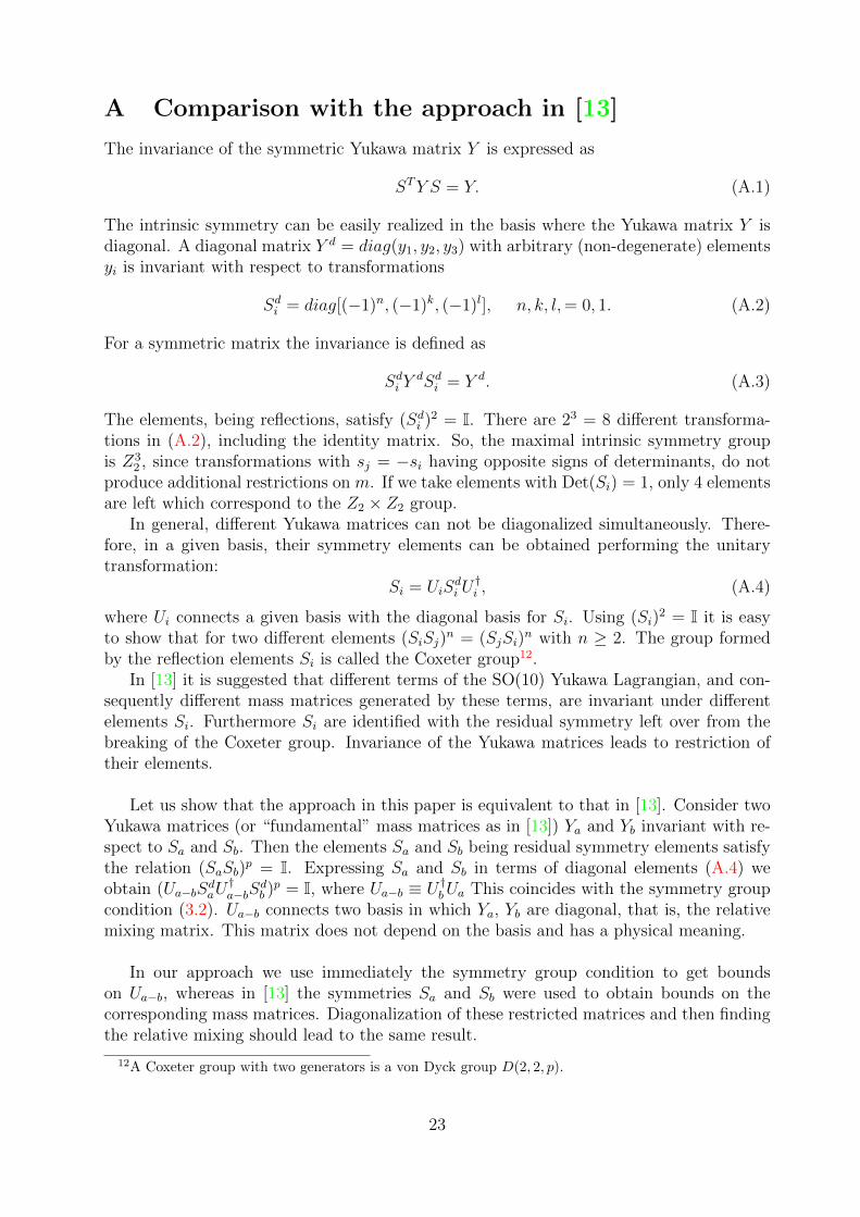
A Comparison with the approach in [13]

The invariance of the symmetric Yukawa matrix Y is expressed as

STY S = Y. (A.1)

The intrinsic symmetry can be easily realized in the basis where the Yukawa matrix Y isdiagonal. A diagonal matrix Y d = diag(y1, y2, y3) with arbitrary (non-degenerate) elementsyi is invariant with respect to transformations

Sdi = diag[(−1)n, (−1)k, (−1)l], n, k, l,= 0, 1. (A.2)

For a symmetric matrix the invariance is defined as

Sdi YdSdi = Y d. (A.3)

The elements, being reflections, satisfy (Sdi )2 = I. There are 23 = 8 different transforma-tions in (A.2), including the identity matrix. So, the maximal intrinsic symmetry groupis Z3

2 , since transformations with sj = −si having opposite signs of determinants, do notproduce additional restrictions on m. If we take elements with Det(Si) = 1, only 4 elementsare left which correspond to the Z2 × Z2 group.

In general, different Yukawa matrices can not be diagonalized simultaneously. There-fore, in a given basis, their symmetry elements can be obtained performing the unitarytransformation:

Si = UiSdi U†i , (A.4)

where Ui connects a given basis with the diagonal basis for Si. Using (Si)2 = I it is easy

to show that for two different elements (SiSj)n = (SjSi)

n with n ≥ 2. The group formedby the reflection elements Si is called the Coxeter group12.

In [13] it is suggested that different terms of the SO(10) Yukawa Lagrangian, and con-sequently different mass matrices generated by these terms, are invariant under differentelements Si. Furthermore Si are identified with the residual symmetry left over from thebreaking of the Coxeter group. Invariance of the Yukawa matrices leads to restriction oftheir elements.

Let us show that the approach in this paper is equivalent to that in [13]. Consider twoYukawa matrices (or “fundamental” mass matrices as in [13]) Ya and Yb invariant with re-spect to Sa and Sb. Then the elements Sa and Sb being residual symmetry elements satisfythe relation (SaSb)

p = I. Expressing Sa and Sb in terms of diagonal elements (A.4) weobtain (Ua−bS

daU†a−bS

db )p = I, where Ua−b ≡ U †bUa This coincides with the symmetry group

condition (3.2). Ua−b connects two basis in which Ya, Yb are diagonal, that is, the relativemixing matrix. This matrix does not depend on the basis and has a physical meaning.

In our approach we use immediately the symmetry group condition to get boundson Ua−b, whereas in [13] the symmetries Sa and Sb were used to obtain bounds on thecorresponding mass matrices. Diagonalization of these restricted matrices and then findingthe relative mixing should lead to the same result.

12A Coxeter group with two generators is a von Dyck group D(2, 2, p).

23

Let us illustrate this using two examples. We will consider the Coxeter group A3. Ithas three generators and the group structure is

(S1S3)2 = I, (S1S2)

3 = I, (S3S2)3 = I. (A.5)

In the first example we take Y10 to be invariant with respect to S10 = S1 and Y126with respect to S126 = S3. From the first group relation in (A.5) it follows that S1 andS3 commute. Therefore the basis can be found in which both S1 and S3 are diagonalsimultaneously. We can take S10 = Sd1 and S126 = Sd3 , where Sd1 and Sd3 are given in (2.9).

Let us underline that in this example it is the commutation of S1 and S3 (which is aconsequence of the group structure relation) that encodes the information about embedding.

As the consequence of symmetries, the matrices should have the following vanishingelements

(Y10)12,13,21,31 = 0 (A.6)

(Y126)13,23,31,32 = 0. (A.7)

They are diagonalized by

U10 =

(eiα10 01×202×1 (U10)2×2

), U126 =

((U126)2×2 02×1

01×2 eiα126

)(A.8)

ThereforeU13 =

(U †10U126

)13

= 0. (A.9)

This result can be obtained immediately from our consideration (3.22). Indeed, in thiscase the generators S1 and S3 are involved, so we fix the element U13. In this example p = 2and k = 1 that lead according to (3.22) to U13 = cos (π/2) = 0.

In the second example we take again S10 = S1 as the symmetry of Y10 but S126 = S2

as the symmetry of Y126. Now p = 3 (A.5) and the generators do not commute, so theycan not be diagonalized simultaneously. In the basis S10 = Sd1 according to [13] the thirdelement equals

S2 =1

2

−1√

2 −1

... 0 −√

2... ... −1

. (A.10)

This element can be represented as

S2 = USd2U†, (A.11)

where Sd2 = diag(−1, 1,−1) and, as can be obtained explicitly from (A.10) and (A.11), in Uonly the second column is determined: |Uj2| = (1/2, 1/

√2, 1/2)T . The matrix U is nothing

but the relative matrix which connects two diagonal bases for Si. In particular, we have|U12| = 1/2. Again this result can be obtained immediately from our consideration. Sincethe generators involved are S1 and S2, the 1 - 2 element is fixed. For p = 3 and k = 1 (ork = 2) we have from (3.22) |U12| = cos (π/3) = 1/2.

Notice that in the matrix U only one column is determined, and so there is an ambiguityrelated with certain rotations. Also in the first example we could write the symmetry groupcondition as (Sd1S

d3)2 = I, that is, U = I which is consistent with U13 = 0. Again here we

have an ambiguity related to rotations (A.8).

24

References

[1] H. Georgi and S. L. Glashow, “Unity of All Elementary Particle Forces,” Phys. Rev.Lett. 32 (1974) 438.

[2] J. C. Pati and A. Salam, “Lepton Number as the Fourth Color,” Phys. Rev. D 10(1974) 275 Erratum: [Phys. Rev. D 11 (1975) 703].

[3] H. Fritzsch and P. Minkowski, “Unified Interactions of Leptons and Hadrons,” AnnalsPhys. 93 (1975) 193.

[4] R. N. Mohapatra and B. Sakita, “SO(2n) Grand Unification in an SU(N) Basis,”Phys. Rev. D 21 (1980) 1062.

[5] F. Wilczek and A. Zee, “Families from Spinors,” Phys. Rev. D 25 (1982) 553.

[6] B. Bajc, G. Senjanovic and F. Vissani, “B - Tau Unification and Large AtmosphericMixing: a Case for Noncanonical Seesaw,” Phys. Rev. Lett. 90 (2003) 051802 [hep-ph/0210207].

[7] C. S. Aulakh and R. N. Mohapatra, “Implications of Supersymmetric SO(10) GrandUnification,” Phys. Rev. D 28, 217 (1983); T. E. Clark, T. K. Kuo and N. Nakagawa,“A So(10) Supersymmetric Grand Unified Theory,” Phys. Lett. B 115, 26 (1982);K. S. Babu and R. N. Mohapatra, “Predictive neutrino spectrum in minimal SO(10)grand unification,” Phys. Rev. Lett. 70, 2845 (1993) [hep-ph/9209215]; C. S. Aulakh,B. Bajc, A. Melfo, G. Senjanovic and F. Vissani, “The Minimal supersymmetric grandunified theory,” Phys. Lett. B 588, 196 (2004) [hep-ph/0306242].

[8] R. Barbieri, L. J. Hall, S. Raby and A. Romanino, “Unified Theories with U(2) Fla-vor Symmetry,” Nucl. Phys. B 493 (1997) 3 [hep-ph/9610449]; Z. Berezhiani andA. Rossi, “Predictive Grand Unified Textures for Quark and Neutrino Masses andMixings,” Nucl. Phys. B 594 (2001) 113 [hep-ph/0003084]; M. C. Chen and K. T. Ma-hanthappa, “From Ckm Matrix to Mns Matrix: a Model Based on SupersymmetricSO(10) × U(2)(F) Symmetry,” Phys. Rev. D 62 (2000) 113007 [hep-ph/0005292];G. G. Ross and L. Velasco-Sevilla, “Symmetries and Fermion Masses,” Nucl. Phys. B653 (2003) 3 [hep-ph/0208218]; S. F. King and G. G. Ross, “Fermion Masses and Mix-ing Angles from Su (3) Family Symmetry and Unification,” Phys. Lett. B 574 (2003)239 [hep-ph/0307190]; G. G. Ross, L. Velasco-Sevilla and O. Vives, “Spontaneous CPViolation and Nonabelian Family Symmetry in Susy,” Nucl. Phys. B 692 (2004) 50[hep-ph/0401064]; I. de Medeiros Varzielas and G. G. Ross, “SU(3) Family Symmetryand Neutrino Bi-Tri-Maximal Mixing,” Nucl. Phys. B 733 (2006) 31 [hep-ph/0507176];Z. Berezhiani and F. Nesti, “Supersymmetric SO(10) for Fermion Masses and Mixings:Rank-1 Structures of Flavor,” JHEP 0603 (2006) 041 [hep-ph/0510011]; C. S. Aulakhand C. K. Khosa, “SO(10) Grand Unified Theories with Dynamical Yukawa Cou-plings,” Phys. Rev. D 90 (2014) 4, 045008 arXiv:1308.5665 [hep-ph]]; C. S. Aulakh,“Bajc-Melfo Vacua Enable Yukawon Ultraminimal Grand Unified Theories,” Phys.Rev. D 91 (2015) 055012 [arXiv:1402.3979 [hep-ph]].

[9] D. B. Kaplan and M. Schmaltz, “Flavor Unification and Discrete Nonabelian Symme-tries,” Phys. Rev. D 49 (1994) 3741 [hep-ph/9311281]; D. G. Lee and R. N. Mohapatra,

25

“An SO(10) × S4 Scenario for Naturally Degenerate Neutrinos,” Phys. Lett. B 329(1994) 463 [hep-ph/9403201]; R. Dermisek and S. Raby, “Bi-Large Neutrino Mixingand CP Violation in an SO(10) SUSY GUT for Fermion Masses,” Phys. Lett. B 622(2005) 327 [hep-ph/0507045]; C. Hagedorn, M. Lindner and R. N. Mohapatra, “S4

Flavor Symmetry and Fermion Masses: Towards a Grand Unified Theory of Flavor,”JHEP 0606 (2006) 042 [hep-ph/0602244]; S. F. King and C. Luhn, “A Supersymmet-ric Grand Unified Theory of Flavour with PSL(2)(7) × SO(10),” Nucl. Phys. B 832(2010) 414 [arXiv:0912.1344 [hep-ph]]; K. M. Patel, “An SO(10)XS4 Model of Quark-Lepton Complementarity,” Phys. Lett. B 695 (2011) 225 [arXiv:1008.5061 [hep-ph]].

[10] P. M. Ferreira, W. Grimus, D. Jurciukonis and L. Lavoura, “Flavour Symmetries in aRenormalizable SO(10) Model,” arXiv:1510.02641 [hep-ph].

[11] I. P. Ivanov and L. Lavoura, “SO(10) Models with Flavour Symmetries: Classificationand Examples,” arXiv:1511.02720 [hep-ph].

[12] M. C. Chen and K. T. Mahanthappa, “Fermion Masses and Mixing and CP Violationin SO(10) Models with Family Symmetries,” Int. J. Mod. Phys. A 18 (2003) 5819 [hep-ph/0305088]; G. Altarelli and F. Feruglio, “Discrete Flavor Symmetries and Modelsof Neutrino Mixing,” Rev. Mod. Phys. 82 (2010) 2701 [arXiv:1002.0211 [hep-ph]].

[13] C. S. Lam, “Built-In Horizontal Symmetry of SO(10),” Phys. Rev. D 89 (2014) 9,095017 [arXiv:1403.7835 [hep-ph]].

[14] A. Zee, “A Theory of Lepton Number Violation, Neutrino Majorana Mass, andOscillation,” Phys. Lett. B 93 (1980) 389 [Phys. Lett. B 95 (1980) 461]; A. Zee,“Charged Scalar Field and Quantum Number Violations,” Phys. Lett. B 161 (1985)141; A. Y. Smirnov and M. Tanimoto, “Is Zee Model the Model of Neutrino Masses?,”Phys. Rev. D 55 (1997) 1665 [hep-ph/9604370]; C. Jarlskog, M. Matsuda, S. Skad-hauge and M. Tanimoto, “Zee Mass Matrix and Bimaximal Neutrino Mixing,” Phys.Lett. B 449 (1999) 240; [hep-ph/9812282]. P. H. Frampton and S. L. Glashow, “Canthe Zee Ansatz for Neutrino Masses Be Correct?,” Phys. Lett. B 461 (1999) 95 [hep-ph/9906375]; A. S. Joshipura and S. D. Rindani, “Neutrino Anomalies in an Ex-tended Zee Model,” Phys. Lett. B 464 (1999) 239 [hep-ph/9907390]; K. R. S. Balaji,W. Grimus and T. Schwetz, “The Solar Lma Neutrino Oscillation Solution in the ZeeModel,” Phys. Lett. B 508 (2001) 301 [hep-ph/0104035].

[15] C. S. Lam, “Symmetry of Lepton Mixing,” Phys. Lett. B 656 (2007) 193[arXiv:0708.3665 [hep-ph]].

[16] C. S. Lam, “The Unique Horizontal Symmetry of Leptons,” Phys. Rev. D 78 (2008)073015 [arXiv:0809.1185 [hep-ph]].

[17] C. S. Lam, “A Bottom-Up Analysis of Horizontal Symmetry,” arXiv:0907.2206 [hep-ph].

[18] W. Grimus, L. Lavoura and P. O. Ludl, “Is S4 the Horizontal Symmetry of Tri-Bimaximal Lepton Mixing?,” J. Phys. G 36 (2009) 115007 [arXiv:0906.2689 [hep-ph]].

[19] W. Grimus and L. Lavoura, “Tri-Bimaximal Lepton Mixing from Symmetry Only,”JHEP 0904 (2009) 013 [arXiv:0811.4766 [hep-ph]].

26

[20] D. Hernandez and A. Y. Smirnov, “Lepton Mixing and Discrete Symmetries,” Phys.Rev. D 86 (2012) 053014 [arXiv:1204.0445 [hep-ph]].

[21] D. Hernandez and A. Y. Smirnov, “Discrete Symmetries and Model-Independent Pat-terns of Lepton Mixing,” Phys. Rev. D 87 (2013) 5, 053005 [arXiv:1212.2149 [hep-ph]].

[22] R. M. Fonseca and W. Grimus, “Classification of Lepton Mixing Matrices from FiniteResidual Symmetries,” JHEP 1409 (2014) 033 [arXiv:1405.3678 [hep-ph]].

[23] A. Esmaili and A. Y. Smirnov, “Discrete Symmetries and Mixing of Dirac Neutrinos,”Phys. Rev. D 92 (2015) 9, 093012 [arXiv:1510.00344 [hep-ph]].

[24] A. Blum, C. Hagedorn and M. Lindner, “Fermion Masses and Mixings from Dihe-dral Flavor Symmetries with Preserved Subgroups,” Phys. Rev. D 77 (2008) 076004[arXiv:0709.3450 [hep-ph]].

[25] P. Byakti and P. B. Pal, “Coxeter Groups and the Pmns Matrix,” arXiv:1601.08063[hep-ph].

[26] R. M. Fonseca and W. Grimus, “Roots of Unity and Lepton Mixing Patterns fromFinite Flavour Symmetries,” arXiv:1510.01912 [hep-ph].

[27] F. Feruglio, C. Hagedorn and R. Ziegler, “Lepton Mixing Parameters from Discreteand CP Symmetries,” JHEP 1307 (2013) 027 [arXiv:1211.5560 [hep-ph]].

[28] C. Hagedorn, A. Meroni and L. Vitale, “Mixing Patterns from the Groups Σ(nφ),” J.Phys. A 47 (2014) 055201 [arXiv:1307.5308 [hep-ph]].

[29] J. H. Conway and A. J. Jones, “Trigonometric diophantine equations (On vanishingsums of roots of unity)”, Acta Arithmetica 30 (1976) 229.

[30] T. Fukuyama and N. Okada, “Neutrino oscillation data versus minimal supersymmet-ric SO(10) model,” JHEP 0211, 011 (2002) [hep-ph/0205066]; H. S. Goh, R. N. Mo-hapatra and S. P. Ng, “Minimal SUSY SO(10), b tau unification and large neutrinomixings,” Phys. Lett. B 570, 215 (2003) [hep-ph/0303055]; H. S. Goh, R. N. Mohap-atra and S. P. Ng, “Minimal SUSY SO(10) model and predictions for neutrino mix-ings and leptonic CP violation,” Phys. Rev. D 68, 115008 (2003) [hep-ph/0308197];S. Bertolini, M. Frigerio and M. Malinsky, “Fermion masses in SUSY SO(10) withtype II seesaw: A Non-minimal predictive scenario,” Phys. Rev. D 70, 095002 (2004)[hep-ph/0406117]; K. S. Babu and C. Macesanu, “Neutrino masses and mixings in aminimal SO(10) model,” Phys. Rev. D 72, 115003 (2005) [hep-ph/0505200]; B. Bajc,I. Dorsner and M. Nemevsek, “Minimal SO(10) Splits Supersymmetry,” JHEP 0811(2008) 007 [arXiv:0809.1069 [hep-ph]]; A. S. Joshipura and K. M. Patel, “FermionMasses in SO(10) Models,” Phys. Rev. D 83, 095002 (2011) [arXiv:1102.5148 [hep-ph]]; G. Altarelli and D. Meloni, “A non supersymmetric SO(10) grand unified modelfor all the physics below MGUT ,” JHEP 1308, 021 (2013) [arXiv:1305.1001 [hep-ph]].

[31] A. Dueck and W. Rodejohann, “Fits to SO(10) Grand Unified Models,” JHEP 1309(2013) 024 [arXiv:1306.4468 [hep-ph]].

27

[32] C. S. Aulakh, I. Garg and C. K. Khosa, “Baryon Stability on the Higgs DissolutionEdge: Threshold Corrections and Suppression of Baryon Violation in the Nmsgut,”Nucl. Phys. B 882 (2014) 397 [arXiv:1311.6100 [hep-ph]].

[33] X. Chu and A. Y. Smirnov, “Neutrino mixing and masses in SO(10) GUTs with hiddensector and flavor symmetries,” arXiv:1604.03977 [hep-ph].

[34] R. N. Mohapatra and J. W. F. Valle, “Neutrino Mass and Baryon Number Noncon-servation in Superstring Models,” Phys. Rev. D 34 (1986) 1642.

[35] C. Hagedorn, M. A. Schmidt and A. Y. Smirnov, “Lepton Mixing and Cancella-tion of the Dirac Mass Hierarchy in SO(10) GUTs with Flavor Symmetries T(7) andSigma(81),” Phys. Rev. D 79 (2009) 036002 [arXiv:0811.2955 [hep-ph]].

28