Martin Damyanov Aleksandrov

Master Thesis

Heuristics and Policiesfor

Online Pickup and Delivery Problems

Orientador : Pedro Barahona, Professor, CENTRIA, FCT, UNL,Lisbon, Portugal

Co-orientadores : Philip Kilby, Researcher, NICTA, Canberra, AustraliaToby Walsh, Group Leader, NICTA, Sydney, Australia

President : José Júlio Alves AlferesMain referee : Paula Alexandra da Costa Amaral

Referee : Pedro Manuel Corrêa Calvente Barahona

15 October, 2012

Heuristics and Policies for Online Pickup and

Delivery Problems

Martin Damyanov Aleksandrov

Department of Informatics, Faculty of Sciences and Technology,Univesidade Nova de Lisboa

Advisor : Prof. Pedro Barahona, CENTRIA, UNL, Lisbon, Portugal

co-Advisor 1 : Dr. Philip Kilby, NICTA, Canberra, Australiaco-Advisor 2 : Prof. Toby Walsh, NICTA, Sydney, Australia

Submission date : 15 October 2012

Copyright c©2012, Martin Damyanov AleksandrovAll Rights Reserved

Declarations

I, Martin Damyanov Aleksandrov, certify that this master thesis has been written entirelyby me, that is a record of work carried out by me, it has not been submitted in any pre-vious higher degree application and it will not be submitted in any future higher degreeapplication.

I, Martin Damyanov Aleksandrov below referred to as the Student, certify that this pieceof work has been conducted in both the Universidade Nova de Lisboa, Portugal, below re-ferred to as the Institution 1, between February 2012 and October 2012, and the NationalInformation and Communications Technology Research Center of Excellence, NICTA, Aus-tralia, below referred to as the Institution 2, between October 2011 and January 2012.Attention has been taken with respect to both the study and graduate regulations in theInstitution 1 and the working regulations imposed by the Institution 2 as follows:

1. According to the common reguirements for obtaining a higher-education degree,posted by the Institution 1, this work is submitted to and public available at the Depart-ment of Informatics, Faculty of Sciences and Technology, which is part of the Institution 1.

2. According to the conditions of the Visiting Researcher Agreement contract betweenthe Institution 2 and the Student, started at 1 October 2011 and finished at 18 January2012, the Intellectual Property created during the course of this Agreement is property ofthe Institution 2.

Date : Signature of the Student :

I, Pedro Barahona, hereby certify that the Student has fulfilled the conditions of theregulations appropriate for the degree of European Master in Computational Logic in theInstitution 1 and that the Student is qualified to submit the thesis in application forthat degree.

Date : Signature of the advisor :

I, Philip Kilby, hereby certify that the Student has fulfilled the conditions of the regula-tions mentioned in the Visting Researcher Agreement contract and that the Student isqualified to submit the thesis in application for that degree.

Date : Signature of the co-advisor :

In submitting the thesis to the Universidade Nova de Lisboa we understand that we aregiving permission for it to be mabe available for use in accordance with the regulations ofthe University Library for the time being in force, subject to any copyright vested in thework not being affected thereby. We also understand that the title and the abstract will bepublished, and that a copy of this work will be submitted to the Academic Archive, to theAdvisor and to the co-Advisor.

i

Access to Printed copy of the thesis through the University Nova de Lisboa.

Date : Signature of the Student :

Date : Signature of the advisor :

ii

Preface

This Master thesis entitled ”Heuristics and Policies for Online Pickup and Delivery Prob-lems” has been prepared by Martin Damyanov Aleksandrov during the period October 2011to October 2012 at the National ICT Australia and at the Universidade Nova de Lisboa.Martin Damyanov Aleksandrov visited both places under the common study and mobilityregulations of the European Master Program in Computational Logic.

The thesis work was partially supported by the National ICT Australia according to theVisitor Research Agreement contract between NICTA and Martin Damyanov Aleksandrov.The subject of the thesis is to develop new online dynamic algorithms for dispatching thefleet of vehicles for a well-known subclass of Vehicle Routing Problems, viz. Pickup andDelivery Problems, and to extend the current research in this area by possibly contributingto some basic research problems in intelligent transport systems with potential applicationto areas like traffic control, vehicle routing and logistics. It is motivated by a problem arisedin an Australian courier firm and it aims to achieve and to satisfy their necessities as muchas possible.

Next, I would like to thank my thesis advisor, Pedro Barahona, who is a professor at Uni-versidade Nova de Lisboa for his support and interest throughout this project. I have nowserved as Pedro’s master student during the last year and I have enjoyed our collaborationtogether.

I would like to thank professor Toby Walsh and doctor Philip Kilby, who are research leadersat the NICTA’s Neville Roach and Canberra laboratories, respectively. They were support-ing me during the whole time by giving usefull pieces of advice, opinions and comments onthe theoretical and practical aspects of this thesis.

In addition, I wish to specially thank doctor Philip Kilby for providing me technical infor-mation about the state-of-the-art Vehicle Routing Solver, Indigo 2.0, which is implementedby him and it is a property of NICTA. I really appreciate his efforts and usefull pieces ofadvice during the last one year.

Many special thanks to Hanna Grzybowska for providing the NICTA internal reports, col-lected on June 30, September 1 and September 6, 2011. They were very usefull in modellingand understanding the addressed problem in terms of human, fleet and customer resourcesas well as in providing specific details about the working conditions in the company.

iii

I would like also to express thanks to Menkes van den Briel, who is an operational researchprofessional in the optimization group at NICTA. Our discussions significantly contributedfor better understanding the addressed problem.

Lastly, as a master student in such an European program I spent most of my time travellingaround the world. During all this experience my family, Damyan, Svetla and Iliyan, andmy friends were my moral support and I wish to thank them for encouraging me.

Martin Damyanov Aleksandrov

iv

Abstract

In the last few decades, increased attention has been dedicated to a specific subclass ofVehicle Routing Problems due to its significant importance in several transportation areassuch as taxi companies, courier companies, transportation of people, organ transportation,etc. These problems are characterized by their dynamicity as the demands are, in general,unknown in advance and the corresponding locations are paired. This thesis addresses aversion of such Dynamic Pickup and Delivery Problems, motivated by a problem arisenin an Australian courier company, which operates in Sydney, Melbourne and Brisbane,where almost every day more than a thousand transportation orders arrive and need tobe accommodated. The firm has a fleet of almost two hundred vehicles of various types,mostly operating within the city areas. Thus, whenever new orders arrive at the system thedispatchers face a complex decision regarding the allocation of the new customers withinthe distribution routes (already existing or new) taking into account a complex multi-levelobjective function.

The thesis thus focuses on the process of learning simple dispatch heuristics, and lays thefoundations of a recommendation system able to rank such heuristics. We implemented eightof these, observing different characteristics of the current fleet and orders. It incorporates anartificial neural network that is trained on two hundred days of past data, and is supervisedby schedules produced by an oracle, Indigo, which is a system able to produce suboptimalsolutions to problem instances. The system opens the possibility for many dispatch policiesto be implemented that are based on this rule ranking, and helps dispatchers to managethe vehicles of the fleet. It also provides results for the human resources required eachsingle day and within the different periods of the day. We complement the quite promisingresults obtained with a discussion on future additions and improvements such as channelfleet management, traffic consideration, and learning hyper-heuristics to control simple rulesequences.

v

Resumo

Nas ultimas decadas, tem sido dedicada uma crescente atencao a uma subclasse especıficade problemas de roteamento de veıculos, devido a sua importancia significativa em diver-sas areas de transporte, tais como empresas de taxis, empresas de courier, transporte depessoas, transporte de orgaos, etc. Estes problemas sao caracterizados por sua dinamica,ja que os pedidos envolvendo pares de localizacoes sao, em geral, desconhecidos com an-tecedencia. Esta tese trata de uma versao de Problema de Recolha e Entrega Dinamico,motivado por um problema surgido numa empresa de entregas australiana, que atua emSydney, Melbourne e Brisbane, e em que todos os dias sao feitos mais de mil pedidos detransporte de entregas. A empresa tem uma frota de quase 200 veıculos de varios tipos,e opera principalmente dentro das areas urbanas. Sempre que um novo pedido de entregachega ao sistema, os despachantes enfrentam uma decisao complexa quanto a alocacao dosnovos pedidos dentro das rotas de distribuicao (ja existentes ou novas), tendo em conta umafuncao complexa funcao multi-objetivo.

A tese centra-se no processo de aprendizagem de regras de despacho simples, e lanca asbases de um sistema de recomendacao capaz de classificar as heurısticas existentes. Oitodessas foram implementadas, tendo em conta as caracterısticas das encomendas e do estadocorrente de alocacao da frota e encomendas. O sistema incorpora uma rede neural artificial,treinada por dados referentes a 200 dias de actividade, e supervisionada por um oraculo,Indigo, que e um sistema capaz de produzir solucoes sub-otimas para instancias do problema.O sistema abre a possibilidade de implementacao de variadas polıticas de despacho baseadasnuma ordenacao destas regra heurısticas, e fornece indicacoes para os recursos humanosnecessarios em cada dia, e em diferentes perıodos do dia. Os resultados obtidos sao bastantepromissores e sao complementados com uma discussao sobre futuras adicoes e melhorias,tais como canais de gestao de frotas, analise de trafego, e aprendizagem de hiper-heurısticaspara controlar sequencias de regras simples.

vi

List of Abbreviations

1. BAL - Balanced Heuristic.

2. CDVRP - The Capacitated Dynamic Vehicle Routing Problem.

3. CVRP - The Capacitated Vehicle Routing Problem.

4. CUR - Current Orders Heuristic.

5. DARP - The Dial-a-Ride Problem.

6. DPDP - The Dynamic Pickup and Delivery Problem.

7. DPDPTW - The Dynamic Pickup and Delivery Problem with Time Windows.

8. dDVRP - The Delivery Dynamic Vehicle Routing Problem.

9. DVRP - The Dynamic Vehicle Routing Problem.

10. DVRPTW - The Dynamic Vehicle Routing Problem with Time Windows.

11. GEO - Geographical Closeness Heuristic.

12. GIS - Graphical Information Systems.

13. IMM - Immediate Cost Heuristic.

14. MAV - Minimize Vehicles Heuristic.

15. MIN - Minimum Cost Heuristic.

16. ML - Machine Learning.

17. NN - Neural Network.

18. ODPDP - The Online Dynamic Pickup and Delivery Problem.

19. ODPDPTW - The Online Dynamic Pickup and Delivery Problem with Time Win-dows.

20. OSDPDPTW - The Online Stochastic and Dynamic Pickup and Delivery Problemwith Time Windows.

vii

21. PDP - The Pickup and Delivery Problem.

22. PDPTW - The Pickup and Delivery Problem with Time Windows.

23. PDTSP - The Pickup and Delivery Travelling Salesman Problem.

24. pDVRP - The Pickup Dynamic Vehicle Routing Problem.

25. RAND - Random Heuristic.

26. RL - Reinforcement Learning.

27. SHIFT - Shift Profitability Heuristic.

28. STDPDP - The Stochastic and Dynamic Pickup and Delivery Problem.

29. STDVRP - The Stochastic and Dynamic Vehicle Routing Problem.

30. STVRP - The Stochastic Vehicle Routing Problem.

31. SVRP - The Static Vehicle Routing Problem.

32. TSP - The Traveling Salesman Problem.

33. UDVRP - The Uncapacitated Dynamic Vehicle Routing Problem.

34. VRP - The Vehicle Routing Problem.

viii

List of Tables

1.1 Sydney fleet characteristics. . . . . . . . . . . . . . . . . . . . . . . . . . . . 51.2 Bonds standart services. . . . . . . . . . . . . . . . . . . . . . . . . . . . . . 51.3 Bonds extra services. . . . . . . . . . . . . . . . . . . . . . . . . . . . . . . . 6

2.1 VRP constraints. . . . . . . . . . . . . . . . . . . . . . . . . . . . . . . . . . 212.2 Paired and time window constraints. . . . . . . . . . . . . . . . . . . . . . . 222.3 Time slices scenarios. . . . . . . . . . . . . . . . . . . . . . . . . . . . . . . . 24

3.1 Route constraints : regarding the arrival moment. . . . . . . . . . . . . . . 323.2 Route constraints : regarding the new order capacities. . . . . . . . . . . . . 323.3 Minimum Cost constraints. . . . . . . . . . . . . . . . . . . . . . . . . . . . 353.4 Balanced constraints. . . . . . . . . . . . . . . . . . . . . . . . . . . . . . . . 403.5 Current Orders constraints. . . . . . . . . . . . . . . . . . . . . . . . . . . . 423.6 Shift Profitability constraints. . . . . . . . . . . . . . . . . . . . . . . . . . . 433.7 Geographical Closeness constraints. . . . . . . . . . . . . . . . . . . . . . . . 453.8 Minimize Vehicles constraints. . . . . . . . . . . . . . . . . . . . . . . . . . . 463.9 Immediate Cost constraints. . . . . . . . . . . . . . . . . . . . . . . . . . . . 473.10 Weaken constraints. . . . . . . . . . . . . . . . . . . . . . . . . . . . . . . . 483.11 Worst-case complexity assesments. . . . . . . . . . . . . . . . . . . . . . . . 50

4.1 Real and seeming order statistics. . . . . . . . . . . . . . . . . . . . . . . . . 574.2 Once-a-day pooling strategy : cost statistics. . . . . . . . . . . . . . . . . . 674.3 Once-a-day pooling strategy : time performance. . . . . . . . . . . . . . . . 684.4 Once-a-day pooling strategy : global valuation statistics. . . . . . . . . . . . 694.5 Time-zones pooling strategy : global valuation statistics. . . . . . . . . . . . 694.6 Fixed-time-span pooling strategy : global valuation statistics. . . . . . . . . 694.7 Time-zones pooling strategy : global vs. local statistics. . . . . . . . . . . . 714.8 Fixed-time-span pooling strategy : global vs. local statistics. . . . . . . . . 71

5.1 Demand features. . . . . . . . . . . . . . . . . . . . . . . . . . . . . . . . . . 765.2 Schedule current features. . . . . . . . . . . . . . . . . . . . . . . . . . . . . 77

ix

List of Figures

1.1 The distribution of the arriving orders within a single weekday. . . . . . . . 31.2 A specification of Vehicle Routing Problems. . . . . . . . . . . . . . . . . . 11

2.1 Non-homogenous and periodic counting process. . . . . . . . . . . . . . . . 25

3.1 Rasterized area of Sydney. . . . . . . . . . . . . . . . . . . . . . . . . . . . . 44

4.1 Datasets. . . . . . . . . . . . . . . . . . . . . . . . . . . . . . . . . . . . . . 534.2 Order arrival distributions. . . . . . . . . . . . . . . . . . . . . . . . . . . . 534.3 Regression matrix. . . . . . . . . . . . . . . . . . . . . . . . . . . . . . . . . 554.4 Arrivals and weight distributions. . . . . . . . . . . . . . . . . . . . . . . . . 564.5 Comparison of the original and the generated datasets. . . . . . . . . . . . . 574.6 Evaluation procedure. . . . . . . . . . . . . . . . . . . . . . . . . . . . . . . 59

5.1 Neural network general structure. . . . . . . . . . . . . . . . . . . . . . . . . 755.2 Recommendation system scheme. . . . . . . . . . . . . . . . . . . . . . . . . 775.3 Global learning features. . . . . . . . . . . . . . . . . . . . . . . . . . . . . . 785.4 Global and local learning features. . . . . . . . . . . . . . . . . . . . . . . . 795.5 Policy comparison in once pooling strategy. . . . . . . . . . . . . . . . . . . 815.6 Fleet management under πPG policy. . . . . . . . . . . . . . . . . . . . . . . 825.7 Policy comparison in time-zones pooling strategy. . . . . . . . . . . . . . . . 84

x

Contents

1 Introduction 11.1 Motivation . . . . . . . . . . . . . . . . . . . . . . . . . . . . . . . . . . . . 2

1.1.1 Fleet and service description . . . . . . . . . . . . . . . . . . . . . . 41.1.2 Objectives . . . . . . . . . . . . . . . . . . . . . . . . . . . . . . . . . 61.1.3 Summary of our problem as ODPDP . . . . . . . . . . . . . . . . . . 7

1.2 History Notes . . . . . . . . . . . . . . . . . . . . . . . . . . . . . . . . . . . 81.3 Specification of VRPs . . . . . . . . . . . . . . . . . . . . . . . . . . . . . . 101.4 The Vehicle Routing Solver Indigo . . . . . . . . . . . . . . . . . . . . . . . 111.5 Thesis contributions . . . . . . . . . . . . . . . . . . . . . . . . . . . . . . . 131.6 Thesis Structure . . . . . . . . . . . . . . . . . . . . . . . . . . . . . . . . . 14

2 A Framework for DPDP 152.1 The Problem Formulation . . . . . . . . . . . . . . . . . . . . . . . . . . . . 162.2 The Basic VRP . . . . . . . . . . . . . . . . . . . . . . . . . . . . . . . . . . 202.3 Paired Customers and Time Windows . . . . . . . . . . . . . . . . . . . . . 222.4 Switching to a Dynamic Setting . . . . . . . . . . . . . . . . . . . . . . . . . 23

2.4.1 Time slices . . . . . . . . . . . . . . . . . . . . . . . . . . . . . . . . 242.4.2 Prediction model . . . . . . . . . . . . . . . . . . . . . . . . . . . . . 24

2.5 Objective Function . . . . . . . . . . . . . . . . . . . . . . . . . . . . . . . . 252.6 NP-hardness . . . . . . . . . . . . . . . . . . . . . . . . . . . . . . . . . . . 28

3 Simple Dispatch Heuristics 293.1 General Assumptions . . . . . . . . . . . . . . . . . . . . . . . . . . . . . . . 30

3.1.1 Possible routes . . . . . . . . . . . . . . . . . . . . . . . . . . . . . . 323.1.2 Capacity constraints . . . . . . . . . . . . . . . . . . . . . . . . . . . 323.1.3 Additional travel costs . . . . . . . . . . . . . . . . . . . . . . . . . . 333.1.4 Time window urgency . . . . . . . . . . . . . . . . . . . . . . . . . . 333.1.5 Distance measures . . . . . . . . . . . . . . . . . . . . . . . . . . . . 34

3.2 Heuristics . . . . . . . . . . . . . . . . . . . . . . . . . . . . . . . . . . . . . 353.2.1 Minimum cost heuristic . . . . . . . . . . . . . . . . . . . . . . . . . 353.2.2 Balanced heuristic . . . . . . . . . . . . . . . . . . . . . . . . . . . . 403.2.3 Current orders heuristic . . . . . . . . . . . . . . . . . . . . . . . . . 413.2.4 Shift profitability heuristic . . . . . . . . . . . . . . . . . . . . . . . . 423.2.5 Geographical closeness heuristic . . . . . . . . . . . . . . . . . . . . . 443.2.6 Minimize vehicles heuristic . . . . . . . . . . . . . . . . . . . . . . . 45

xi

3.2.7 Immediate cost heuristic . . . . . . . . . . . . . . . . . . . . . . . . . 473.2.8 Random heuristic . . . . . . . . . . . . . . . . . . . . . . . . . . . . . 483.2.9 Weaken heuristic constraints . . . . . . . . . . . . . . . . . . . . . . 48

3.3 Summary . . . . . . . . . . . . . . . . . . . . . . . . . . . . . . . . . . . . . 49

4 Heuristic Experiments 514.1 General Assumptions . . . . . . . . . . . . . . . . . . . . . . . . . . . . . . . 524.2 Benchmark Datasets . . . . . . . . . . . . . . . . . . . . . . . . . . . . . . . 52

4.2.1 Original Dataset . . . . . . . . . . . . . . . . . . . . . . . . . . . . . 524.2.2 Arrival distributions . . . . . . . . . . . . . . . . . . . . . . . . . . . 534.2.3 Regression analyses . . . . . . . . . . . . . . . . . . . . . . . . . . . 544.2.4 Predictor distributions . . . . . . . . . . . . . . . . . . . . . . . . . . 554.2.5 Generated datasets . . . . . . . . . . . . . . . . . . . . . . . . . . . . 56

4.3 An Experimental Framework . . . . . . . . . . . . . . . . . . . . . . . . . . 584.3.1 Initial schedule . . . . . . . . . . . . . . . . . . . . . . . . . . . . . . 584.3.2 Suboptimal schedule . . . . . . . . . . . . . . . . . . . . . . . . . . . 584.3.3 Evaluation procedure . . . . . . . . . . . . . . . . . . . . . . . . . . 594.3.4 Request sequences . . . . . . . . . . . . . . . . . . . . . . . . . . . . 604.3.5 Solutions and partial solutions . . . . . . . . . . . . . . . . . . . . . 604.3.6 Heuristic correctness . . . . . . . . . . . . . . . . . . . . . . . . . . . 62

4.4 Experimental Results . . . . . . . . . . . . . . . . . . . . . . . . . . . . . . . 634.4.1 Once-a-day strategy . . . . . . . . . . . . . . . . . . . . . . . . . . . 644.4.2 Time-zones strategy . . . . . . . . . . . . . . . . . . . . . . . . . . . 644.4.3 Fixed-time-span strategy . . . . . . . . . . . . . . . . . . . . . . . . 654.4.4 Cost . . . . . . . . . . . . . . . . . . . . . . . . . . . . . . . . . . . . 664.4.5 Time performance . . . . . . . . . . . . . . . . . . . . . . . . . . . . 674.4.6 Correctness . . . . . . . . . . . . . . . . . . . . . . . . . . . . . . . . 684.4.7 Global vs. local correctness . . . . . . . . . . . . . . . . . . . . . . . 70

4.5 Summary . . . . . . . . . . . . . . . . . . . . . . . . . . . . . . . . . . . . . 72

5 Learning Experiments 735.1 Machine Learning . . . . . . . . . . . . . . . . . . . . . . . . . . . . . . . . . 735.2 Neural Network . . . . . . . . . . . . . . . . . . . . . . . . . . . . . . . . . . 745.3 Features, Datasets and System Scheme . . . . . . . . . . . . . . . . . . . . . 765.4 Dispatch Policies . . . . . . . . . . . . . . . . . . . . . . . . . . . . . . . . . 79

5.4.1 Policy MaxSumPG . . . . . . . . . . . . . . . . . . . . . . . . . . . . 795.4.2 Policy MinSumPG . . . . . . . . . . . . . . . . . . . . . . . . . . . . 805.4.3 Policy MaxSumPLG . . . . . . . . . . . . . . . . . . . . . . . . . . . 805.4.4 Policy MinSumPLG . . . . . . . . . . . . . . . . . . . . . . . . . . . 80

5.5 Experimental Results . . . . . . . . . . . . . . . . . . . . . . . . . . . . . . . 805.6 Summary . . . . . . . . . . . . . . . . . . . . . . . . . . . . . . . . . . . . . 85

xii

6 Future Perspective 866.1 Cross-utilization . . . . . . . . . . . . . . . . . . . . . . . . . . . . . . . . . 876.2 Traffic Congestion . . . . . . . . . . . . . . . . . . . . . . . . . . . . . . . . 886.3 Hyper-heuristics . . . . . . . . . . . . . . . . . . . . . . . . . . . . . . . . . 886.4 Channel fleet management . . . . . . . . . . . . . . . . . . . . . . . . . . . . 88

A Appendix References 90

Bibliography 95

xiii

Chapter 1

Introduction

Introduction is a new beginning.by Martin Aleksandrov

The chapter starts with the presentation of the motivational background behind our workby describing the problem source and its characteristics. We map the task in our attentioninto a problem of the well-known subclass of Vehicle Routing Problems (VRPs), namelyPickup and Delivery Problems (PDPs). As we deal with a courier company, where the newdemands arrive dynamically, it would be beneficial to take into consideration their dynam-icity as well as to consider a prediction model of these demands, which tells us when andwhere a new errand would occur with some degree of certainty.

We bring the reader closer to the class of VRPs by surveying some of the relevant literaturesources and by discussing some of the efforts put in such problems. The history notes donot give a total overview of such problems but we attemp to track the research line inthis area along the years and give an additional motivation to our project. In parallel, wehighlight the features of our work in order to support it with a more clear distinction fromthe previous work.

The next section presents a specification of the VRPs. In the past many people have spec-ified these problems and we do not argue that our criterion is a total or an unique one,rather we present it to narrow the attention of the reader to the task we deal with. Wecapture our characterization of the VRPs with a figure, depicting the relations between thedifferent subclasses and underlining the assumptions made within each one of them.

We continue this introductory chapter with the description of the oracle used along thethesis, namely VRP Solver Indigo 2.0. It has been implemented in NICTA and it is aproperty of NICTA. We present the general architecture phases of Indigo and we shortlydiscuss the methodologies used in each one of them. Finally, we give a brief summary ofthe thesis contributions and thesis structure.

1

1.1 Motivation

A local courier firm has approached NICTA about providing a decision support tool toschedule their pick-up and deliveries. Bonds Express is a part of Bonds Transport Group,which has been established in 1966 and has recently grown to become a specialist multidis-cipline, Australian transport and 3PL provider. It is privately owned and it is dedicated toproviding a total quality transport solution to its customers. It operates fast, secure and re-liable express courier and taxi-truck services mostly within the areas of Sydney, Melbourneand Brisbane. Offering a full range of services, Bonds has the ability to meet standart andurgent delivery needs. They also offer highly competative rates for interstate and interna-tional deliveries1.

Next, we describe the scope of the problem arised in Bonds Express Couriers. The dis-patchers in the company control six channels of information flow between the customers,requesting services, and the drivers executing these services. Each dispatcher manages onechannel, which does not correspond to a region, rather to a range of vehicle types. Cur-rently, the dispatchers estimate themselves the most probable service time per job. Therole of the dispatchers is of essential importance as we can view them as the distributionpoints in such information flows. At the same time they obey certain constraints related totheir working conditions, namely they have a limited scheduling horizon and they cannotexchange information between each other. The drivers can refuse to do an assigned joband they are very selective and picky about the tasks to be performed. Currently, theorder of the requests to be serviced is decided by the drivers, which means they participatein constructing their own route. The dispatchers wish to have a higher control on this or-der and to navigate the drivers towards their next destinations more precisely and routinely.

The information about vehicle locations arrive at the center dispatching unit via GPS ev-ery 3 minutes. The other direction of communication is realized via mobile text messages,which can be ambigious. Therefore, the dispatchers wish to have an improved and frequentcommunication with the drivers. The company has a policy of accepting all incoming jobrequests, even though they know they might not be able to satisfy the customer on-timerequirements. In this case, the penalty for arriving too late is reflected in the profit formaking the particular job. They pay the driver from the moment he picks up the first ordertill the moment they drop off the last one. They must pay the minimum hourly rate to thedriver and keep the right to send him back home at any time. Once a driver is sent homehe is no more available to the dispatchers on that day.

The fleet obeys specific limitations not only with respect to the physical characteristics ofits vehicles, but also with respect to the driver contracts. According to the current work-ing conditions, drivers are allowed to work a maximum of 8 hours per day. If this time isexceeded some extra regulations are in force, which are not within our scope. Thus, eachvehicle has a fixed time working horizon. In the next section, we present additional informa-tion about the fleet characteristics, i.e. type, commodities, average velocity per kilometreand an estimate of the average running cost.

1http://www.bondscouriers.com.au/

2

The demands themselves must obey several restrictions. They should be serviced withinlimited response time, which depends on the customer as well as on the type of the chosenservice. Recall, that our orders are paired and composed of a pick-up and delivery requests.Thus, a natural constraint is having the pick-up location to precede the delivery one. Be-sides the geographical and the time preference data attached to all the incoming requests,they also include information about their commodity characteristics. In practice, this wouldallow us to build loading and unloading process specifications for each vehicle. The latteris important as it could significantly reduce the service time at a customer location andfurther optimize our objectives.

During a working day many dynamic orders arrive at the company. As expected, in thedifferent parts of the day the order arrival frequency is different and, consequently, thetotal workload of the fleet would differ in these periods. Based on the distribution of thenew order arrivals along the day we define four time zones. Each of them has specificcharacteristics such as distribution, average job commodity characteristics, most used typeof vehicle within a particular zone, average travel time between clients and others, whichwe discuss later on. The proposed definition of time zones, which is based on the provideddata is depicted in Figure 1.1 1, where time ti is the moment the zone i starts. The divisionis as follows : Night (time zone 1), Morning pick hours (time zone 2), Day (time zone 3)and Evening pick hours (time zone 4). Figure 1.1 also shows the demand arrival rate duringa single working day and it also includes the orders requested for the following days.

Figure 1.1: The distribution of the arriving orders within a single weekday.

Using this distribution we can prepare a routing and scheduling plan for the entire day, foreach time zone, for a fixed time span or whenever a predefined event happens. This recalcu-lation of the plan can be made on the basis of additional information, either revealed to the

1According to the NICTA internal report from June 30, 2011.

3

decision maker or based on historical basis. Once specified the frequency of rerouting andrescheduling of the current plan, the rules regarding the diversion of freight vehicles need tobe defined. For modelling purposes, it has been assumed that the drivers can communicatewith the dispatchers via communication devices installed only at client locations. As aconsequence, while they are serving a client they can be informed about the changes in therouting and scheduling plan. However, each vehicle must perform the lastly assigned service.

Once a shipping parcel has been picked up, its delivery location has to be visited by thesame vehicle in the same day. Hence before modifying the current sequence of clients tovisit a list of compulsory delivery customers needs to be created, which cannot be shiftedto any other route, but can be visited in an order different from the originally established.Although, we do not assume a possible cross-utilization amongst vehicles, in practice itmight be an important issue.

1.1.1 Fleet and service description

In our work we concentrate on the area around Sydney, which is lying between −33.4 and−34.4 latitude, and between 150.67 and 151.67 longitude coordinates. It covers the mainmetropolitan area as well as its surrounding regional centers. The core Sydney fleet iscomprised of approximately 200 vehicles that range from CBD bicycles to vans and flat-tops to 14 tonne trucks and semi-trailers. We summarize the types of vehicles operatingwithin the Sydney urban network in the Table 1.1 1. There are 17 types of vehicles, eachone described with the following features :

• vehicle type

• vehicle code

• maximum number of pallets a type is able to accommodate

• maximum load a type is able to accommodate

• number of available vehicles of the given type

• estimate of the average cost per kilometer the company pays to have a vehicle ofthat type on the road

• average velocity of a vehicle

The cost was estimated taking into account the type of vehicle, its average gas and/or oilconsumption per a hundred kilometres, the additional expenses when a vehicle is full andthe average gas price within the Sydney area for the months between April and June, 20122. The velocity considered is according to the urban city speed regulations with respect tothe vehicle type, assumed an area without traffic congestion.

1According to the NICTA internal report from June 30, 2011.2http://www.carbonblack.com.au/dealer/50/cheapest-petrol-prices.aspx

4

#Type ofvehicle

Vehiclecode

Max.weight[kgs]

Max.pallets

NumberCost

[$/km]

Vehiclespeed[km/h]

1 Pushbike PB 2 0 6 0.02 15

2 Motorbike MB 25 0 6 0.07 35

3 Car CAR 75 0 4 0.12 50

4 Station Wagon SW 250 0 8 0.17 50

5 Small Van SV 500 0 5 0.26 50

6 Large Van 1V 1000 0 68 0.4 50

7 1 Tonne Tray 1T 1000 2 34 0.44 50

8 2 Tonne Tray 2T 2000 4 18 0.87 50

9 2 Tonne Van 2V 2000 2 4 0.73 50

10 2 Tonne Pan 2P 2000 2 2 0.73 50

11 4 Tonne Tray 4T 4000 6 10 1.5 50

12 4 Tonne Taut 4TA 4000 6 1 1.5 50

13 6 Tonne Tray 6T 6000 8 4 2.3 50

14 8 Tonne Tray 8T 8000 10 17 2.95 50

15 12 Tonne Tray 12T 12000 12 3 4.76 50

16 14 Tonne Tray 14T 14000 14 1 5.49 50

17 14 Tonne Pan 14P 14000 14 1 5.49 50

Table 1.1: Sydney fleet characteristics.

Standard Service Maximum Delivery time

Standard Courier 3 hours

Priority Courier 1 hour and 55 minutes

Express Guaranteed arrangement on the phone

Table 1.2: Bonds standart services.

The fleet tries to satisfy each customer necessity through a variety of standard and extraservices. The standard services are summarized in Table 1.2 together with the maximumdelivery times within which they should be performed, and the extra services are describedin Table 1.31. The actual average delivery times are significantly less than the maximumquoted, although these are subject to traffic and weather conditions. Extra time of approxi-mately 25% should be allowed for meeting deadlines of deliveries of more than 30 kilometresdriving distance and to destinations outside the metropolitan area2. Recall, that the con-ditions of the type of service are discussed with the customer when the demand is beingrequested and they are incorporated in his time preferences.

1According to the NICTA internal report from June 30, 2011.2http://www.bondscouriers.com.au/

5

Extra Service Description

Bicycle Courierfast, reliable and economic service;

consignment size and weightlimitations

Motorbike Courier

faster than a car or a van at normalcourier charges; covers limited areaand includes consignment size and

weight limitations

Taxi Truck Service

slower than most of the fleet memberand at higher charges in both travel

and service aspects; significantconsignment size and weight capacity

Taxi Truck Priorityfaster than Taxi Truck Service, but

on a higher hourly and kilometer rate

Intrastate, Interstate and Overseassame day, overnight air and road

freight

Table 1.3: Bonds extra services.

1.1.2 Objectives

Here we list the objectives the company is willing to achieve. As this master thesis is a partof a bigger project, whose final goal is to deliver an end-user product to the company, i.e.a decision supporting tool, we concentrate on those aims more relevant to our problem.

1. The minimum number of requests assigned to a vehicle type in order to ensure prof-itability for the shift.

2. The time of active performance of a vehicle type, i.e. without waiting times.

3. The average number of requests per driver per vehicle type.

4. The average schedule duration per driver per vehicle type.

5. The degree of dynamism of the addressed problem.

6. The maximization of simultaneous utilisation of vehicles for multiple deliveries.

7. The improvement of the overall fleet utilization.

8. The capacity of any vehicle that should not be exceeded at any time.

9. The satisfaction of the customers, which is improved by ensuring more on-time ser-vices.

10. The quality of the scheduling plan, i.e. the number of late jobs performed a given day.

6

11. The number of contracted drivers in relation with the jobs performed for a single day.The objective is to minimize the former and to maximize the latter.

12. The number of drivers to be contracted at the beginning of the working day and thenumber of those sent home along the day.

13. The order, in which a driver visits the clients.

14. The final cost to be minimized.

1.1.3 Summary of our problem as ODPDP

In this subsection we extract all relevant information from the informal specification givenabove in order to concentrate on the problem in hands. We restrict the problem to theSydney fleet of the company and services only within the metropolitan area and its sur-ronding regional centers. We consider a heterogenous fleet of 192 vehicles, each with a type,capacities, running cost and running velocity described in Table 1.1. Each vehicle has ahome location which is where the day starts and ends. Once a vehicle leaves its depot, thefirm pays a cost per hour until the vehicle returns at the end of its shift. We consider a shiftlength of minimum 1 and maximum 8 hours per day. Also each vehicle type has a givencapacity in terms of weight and number of pallets. There are hard constraints on the totalweight and the total number of pallets that can be carried at any one time.

The problem is dynamic as the orders can arrive at any time. Each order is described byan order id, order arrival time, order weight, order pallets, pick-up location, earliest pick-uptime, latest pick-up time, delivery location, and latest delivery time. The earliest pick-uptime is a hard constraint as the package is assumed not to be ready before this time. Wemay require vehicles to wait at a location till the earliest pick-up time constraint is sat-isfied. The latest pick-up and delivery times are soft constraints and there are piecewiselinear penalty terms in the objective for violating these constraints. There are service timesfor each location to account the time needed to collect or deliver the requested parcel. Dueto the lack of more precise information about the fleet and order commodity dimensionswe could not build loading and unloading specifications for the vehicle types, and assume3 minutes of service time for goods less that 250 kilograms and 10 minutes 1, otherwise.The pick-up and delivery times are defined by the customer. They express his preferencesand can be arranged during the booking time. The type of service needed is also taken intoaccount when these preferences are discussed. In addition, we suppose orders are scheduledwithin a single day, assuming that some of them have been requested some days before. Inreality, we may hold requests at the end of the day for the next morning, afternoon, eveningor even for several subsequent days.

Importantly, the routing is supposed to be online. Whilst we may have a tentative schedulefor all current orders, we only commit to a pick-up or delivery when the previous demandhas been executed. A vehicle can be diverted at a client location, but not along its waybetween any two consecutive visits. The driver may consult with a dispatcher about his

1According to the NICTA internal report from June 30, 2011.

7

next destination via PDA device. Finally, we do not allow any load to be stored at any ofthe depot, customer or intermediate locations. In practice, a vehicle could deliver a packageto some place, called store, where another or even the same vehicle will arrive later andcollect the particular good. The last would be an interesting extension to our work, butsince our focus is centered on learning dispatch decisions we do not consider this issue.

1.2 History Notes

A Vehicle Routing Problem (VRP) can be defined as a problem of finding the optimal routesof delivery or collection from one or several depots to a number of cities or customers, whilesatisfying some constraints. Collection of household waste, gasoline delivery trucks, goodsdistribution, snowplough and mail delivery are the most used applications of the VRP. TheVRP plays a vital role in distribution and logistics. Huge research efforts have been de-voted to studying the VRP since 1954 when Dantzig and Ramser [17] have described theproblem as a generalised problem of Travelling Salesman Problem (TPS). Since this pointonwards a tremendous amount of research work has been concentrated on the comparisonbetween practically expensive exact methods and heuristic approaches. Some of the workon this subject after the eighties are Christofides et al., 1981 [12], who used spanning treeand shortest path relaxations to solve a number of instances derived from the literature.Desrochers, Lenstra and Savelsbergh in 1990 [18] (Laporte, 1992 [42]) surveyed main exactand approximate algorithms developed for a VRP, at a level appropriate for a first graduatecourse in combinatorial optimization. Later on Baldacci et al. in 2008 [5] introduced anexact algorithm for the capacitated version of a VRP (CVRP) based on the set partitioningformulation and additional cuts that correspond to capacity and clique inequalities in theVRP graph. Baldacci also discussed some recent advances the same year (2008) in [4].Apart from the classical formulation and its variants also many efforts have been made inmodelling specific optimization problems by means of VRP. For instance, Dong et al. 2011described a variant of VRP in Flight Ticket Sales Companies for the service of free pickupand delivery of airline passengers to the airport (see [20]).

An important characteristic of a VRPs is whether the information of the demands is knownin advance. From this perspective, the class of VRPs can be split into Static VRPs(Berbeglia et al., 2007 [7]) and Dynamic VRPs (Psaraftis, 1988 [51], Kilby et al., 1998[38] and Larsen et al., 2002 [44]). The latter type captures some specificities appearing inthe real-case studies, which usually a static approach disregards. The main difference isthat in the static problem all the information about the demands is assumed to be availablein advance. On the contrary, a dynamic instance tries to capture the dynamic behaviourof these client requests, as they typically arrive as the day progresses. Hence, its probleminstances must be solved a large number of times and, moreover, in a reasonable time. Es-pecially, in the areas such as taxi-companies, urgent transportation services (people (DARP,Cordeau and Laporte, 2003 [14]), orgar freights (Awasthi and Sandholm, 2009 [3]), etc.),etc. many Static VRP must be solved and further analyzed. The last could be a difficulttask due to the NP-hard nature of these problems. Thus, many researchers and practitionersdivert their attention towards heuristic and look-ahead approaches (Mes et al., 2010 [45])for the DVRP. Many papers have been written on this VRP variant (Mitrovic-Minic et al.

8

2004, [41]). Also the limited knowledge of the incoming demands motivated people to takea close look over the heuristics for Stochastic VRPs (STVRP). Swihart and Papastavrou[55], 1999, considered demands arriving according to a Poisson process. In 2006, Ichoua([32]) exploited a strategy based on a probabilistic knowledge about future requests in or-der to predict where such a stochastic event would occur. Such approaches usually improvethe fleet management. Later on Hvattum et al. [31], 2007, implemented a Branch-and-Regret heuristic for Stochastic and Dynamic VRP (STDVRPs). Several other practicallyimportant variants such as DVRP with Time Windows (DVRPTW), DVRP with Pick-Ups(pDVRP), DVRP with Deliveries (dDVRP), DVRP with Pick-Ups and Deliveries (DPDP,Parragh et al. 2008 [50]) and Capacitated DVRP (CDVRP, Kopmanz et al. 2001 [40],Ganapathy et al. 2009 [23], Chandran and Raghavan, 2008 [11]) as well as UncapacitatedDVRP (Angelelli et al. 2007 [1]) have also been investigated thoroughly.

The class closer to this thesis is a variant of DPDP. Its instances are characterized withadditional considerations regarding the demands, e.g. the deliveries are paired and theymust be executed in a particular order (i.e. the pickup location to be visited before thedelivery one). In other words, objects or people have to be transported between an originand a destination. Moreover, issues related to the order arrival dynamicity and to antici-pating future demands should be taken into account, and therefore we consider Stochasticand Dynamic PDP (STDPDP). Furthermore, the class of PDPs can be classified into threedifferent groups. The first group consists of many-to-many problems, in which any vertexcan serve as a source or as a destination for any commodity. An example of a many-to-many problem is the Swapping Problem (Anily and Hassin, 1992 [2]). In this problem,every vertex may initially contain an object of a known type of commodity as well as adesired type of commodity. The problem consists of constructing a route performing thepickups and deliveries of the objects in such a way that at the end of the route, every vertexpossesses an object of the desired type of commodity. Problems in the second group arecalled one-to-many-to-one problems. In these problems commodities are initially availableat the depot and are destined to the customer vertices; in addition, commodities available atthe customers are destined to the depot. Finally, in one-to-one problems, each commodity(which can be seen as a request) has a given origin and a given destination. Problems ofthis type arise, for example, in courier operations and door-to-door transportation services.Thus, our problem can be classified as one-to-one PDP. In addition, we assume customerpreferences on time windows (PDPTW, Mitrovic-Minic, 1998 [47] and DPDPTW, Mitrovic-Minic et al., 2004 [43]) and stochasticity (STDPDP, Chun-Mei, 2011, [13]).

Moreover as the problem instances are revealed incrementally our focus is on Online DPDPTW(Jaillet and Wagner, 2008 [35]). To the best of our knowledge no research work addressesthe exact problem we focused on, i.e. Online Stochastic and Dynamic Pickup and Deliv-ery Problem with Time Windows (OSDPDPTW). More detailed specification can be givenregarding the fleet dimensions such as the number of the fleet members, i.e. single-vehicleDPDPs (Swihart and Papastavrou, 1999 [55], and Gribkovskaia, and Laporte in 2008 [26])and multi-vehicle DPDPs, investigated by Jaillet et al. in [34], 2004 and Dessouky, andLu the same year [19]. Besides the number of vehicles, their type as well as their homelocations, so-called depots, also have attracted significant research interest. In [33], 2000

9

Irnich studied the multi-depot PDP with a single hub and heterogenous fleet. He focusedon problems where all possible routes can easily be enumerated, i.e. the problem primar-ily considers the assignment of transportation requests to routes. The hub serves as aconsolidation point which often assumes short routes between it and the locations in thetransportation network, i.e. involve only one or very few customers. The rationale for thisone is in the narrow time windows as well as in the high quantities, which make it pos-sible to fully load a vehicle at one customer. Recall, the Bonds Express Couriers has atits disposal a heterogenous fleet, whose members have their own depot. Consequently, thevariant we consider is a multi-depot OSDPDPTW. In addition to the quantitave and typedescription of the fleet a significant attention is devoted to the commodity dimensions of thefleet members. For example, Hernandez-Perez and Salazar-Gonzalez in 2005 ([28]) stud-ied the multi-commodity version of PDTSP, while in 2011 ([52]) Psaraftis explored exactlydynamic programming solutions for the multi-commodity PDP when one or two vehiclesare available. In this thesis we assume a fleet, which has several commodity dimensions.In our case these are the number of pallets and the weight a particular order is composed of.

We are interested specifically in learning dispatch policies to control the fleet of vehiclesonline, rather than using an offline approach. We are not aware of much research in thisprecise setting. Inspired by this and the real case-study arisen in the courier company wedesigned a recommendation system, which applies dispatch rules whenever a new errandarrives taking into account the current parameters of the overall fleet. The decisions madeby the system also take into account the possibility of unreserved demands to occur. Thereare several attempts to dispatch the fleet of vehicles, which we report next. For instance,Cortes et al. (2008, [15]) applied a hybrid-predictive control for fixed-fleet size DPDPsincluding traffic congestion, incorporating future information regarding unknown demandsand expected traffic conditions. Also Gendreau et al. (2006, [24]) proposed neighborhoodsearch heuristics to optimize the planned routes of vehicles in a context where new re-quests, with a pick-up and a delivery location, occur in real-time. Their study is based onejection chains technique and, furthermore, they investigate the impact of a master-slaveparallelization scheme on the optimization process. Two years later, in 2009, Beham et al.([6]) considered agent-based simulation of dispatching rules in DPDP. This work treats thetopic of solving dial-a-ride problems. A simulation model is introduced that describes howan agent is able to satisfy the transportation requests using a complex dispatching rule,which is optimized by metaheuristic approaches. The authors are using fitness function inorder to evaluate the quality of the agent state.

1.3 Specification of VRPs

In this section we present a specification of the VRP subclass of optimization problems weare dealing with in this thesis. The graph of Figure 1.2 with top node ”Vehicle RoutingProblems” follows the historic introduction of the previous section and provides a clearview on how a given general VRP instance could be specified. We do not argue that ourpresentation is unique as there are many other possible classificators that take into accountother problem features. For instance, a vehicle diversion is one of them: a particular vehiclecan decide to visit a new, previously-unknown location on its way towards some previously-

10

known customer. Another issue we omitted is related with the traffic congestion. On couldargue that the traffic is important feature in areas such as courier, cap companies, etc. anda problem instance could be classified with respect to the intensity of the traffic conditions.To emphasize the instance we deal with, we draw a blue line starting from the root, passingthrough the nodes matching our assumptions, and it ends into several nodes describing someof the general fleet, customer and dynamic features taken into account during modellingthe real case-study.

Vehicle Routing Problems

Static VRPDynamic VRP

(Nondeterministic& Stochastic VRP)

VRPwith

Pickups

VRPwith

Deliveries

VRPwith

Pickups & Deliveries

Many-to-many One-to-many-to-oneOne-to-one

Single-vehicle Multi-vehicle

Homogenoues

Fleet

Heterogenous

Fleet

With

Time Windows

Without

Time Windows

Single-request Multi-request

Figure 1.2: A specification of Vehicle Routing Problems.

1.4 The Vehicle Routing Solver Indigo

Here, we give a brief description of the VRP solver Indigo version 2.0 used along this work.In order to obtain meaningful results allowing us to rate the implemented dispatch rulesa large number of suboptimal solutions are needed. Each solution is composed of vehicleassignments as well as the precise timing of their executions. For this purpose, we usedIndigo as an oracle, able to produce such timetables when given a particular specifiction of

11

a VRP instance. The process of creating such a schedule, which helps in managing the fleetof vehicles, is divided into two main phases. During the first, the system constructs visitingassignments to each vehicle subject to the following requirements :

1. It returns ordered routes.

2. The objective could be specified in terms of distance, time or cost measures.

3. It allows arbitrary customer requests, i.e. pickups and deliveries.

4. A single time window for each customer location.

5. Vehicle limits, i.e. maximal capacities.

6. Vehicle availability window, i.e. the time when a particular vehicle is available. Thestart and end locations are arbitrary.

7. Compatibility constraints.

8. Metrics (i.e. distance, time, cost) represented as a matrix of values between any twolocations.

9. Only one route per vehicle is allowed.

The usual way to construct a solution to routing problems is via insertion. That is, therepresentation of the emerging routes is kept internally. The system first chooses a visit toinsert, then looks at all possible insertion points and when the best such point is selected,it updates the routes, and continues by considering the next visit. The insertion methodsimplemented are basically weighted combinations of visit characteristics such as :

1. The number of routes where the visit can be feasibly inserted into.

2. The width of the time window(s).

3. The size of the load(s).

4. The minimum insertion cost.

5. The insertion regret cost (difference between best and second-best cost).

6. The amount the insertion reduces the slack (spare time) in the best route.

Once the initial routes are built, they are subsequently improved by means of local searchduring the second phase of constructing the final schedules. The VRP Solver searches for aneighbour solution (defined according to one of a number of local search neighbourhoods)that is both feasible according to the basic constraints, and cost-reducing. When one isfound, Indigo calculates the true cost and feasibility of a possible implementation usinginvariants. This is the cost which would then be used to determine whether the change isaccepted. The following local search neighbourhoods are realized in Indigo :

1. 2-opt assumes moving a pair of consecutive visits to another route or to the same one,but at a different part, in both forward and reverse orientations.

12

2. Or-opt considers moving a sequence of k consecutive visits to another route or anotherpart of the same route, in both forward and reverse orientations. The number k usuallyis of an order between 5 and 10.

3. Large Neighbourhood Search partially deconstructs (removes visits from the solution)and then re-constructs the solution. To do the last it uses the construction methodslisted above. Thus, in effect a call to the VRP Solver with a partially-constructed so-lution is made, but acceptance of the resulting solution depends on the meta-heuristicbeing used. The designed meta-heuristics for that purpose are Hill-climbing - bestfirst, Hill-climbing - first-found, Adaptive tabu search, Limited Discrepancy Searchand Simulated Annealing.

The quality of the final schedules in terms of the specified objective depends partly on thenumber of the improvement iterations performed during the second implementation phase.In our work, all the solutions produced are improved under the same parameter settings,which allow us to use them as an uniform baseline during the experiments. The parameterswe used to build solutions are Large Neightbourhood Search ([16]) combined with the Sim-ulated Annealing ([21]) meta-heuristic, for a total number of 10000 improvement iterations.

1.5 Thesis contributions

Here we summary the contributions we made in the field of Vehicle Routing Problems. AnAustralian courier company has approached NICTA to provide a decision-support tool formanaging their deliveries. Motivated by this problem we concentrated on the developmentof a recommendation module for this tool. We first introduced a theoretical frameworkwithin which we conducted our research. Although, there are many such frameworks in theliterature, we adopted one fitting best to our needs. We modelled the real case-study as anOnline Stochastic and Dynamic Pickup and Delivery Problem. The latter VRP variant hasbeen investigated thoroughly within the last years, however, not much research attentionconsiders the exact assumptions we made.

In order to support the company workforce in dispatching the fleet we implemented eightonline dispatch heuristics, which take into account the current status of the fleet togetherwith the new demands. This set is composed of the rules Minimum Cost, Balanced,Current Orders, Shift Profitability, Geographical Closeness, Immediate Cost,Minimize Vehicles and Random. For each rule we presented its algorithm as well asdiscussed its correctness and complexity.

Next, we generated 330 days of benchmark data, which were used during the experiments.The datasets were generated with a particular attention on the problem in hand (a versionof Pickup and Delivery Problem). We continued with the evaluation of the dispatch rulesover a hundred of these artificially generated benchmarks. For this purpose we introducedseveral valuation measures, i.e. precise and type global and local measures. The entireprocedure was performed under three pooling scenarios, i.e. (once, time-zones and fixed-time-span) for both cases of presence and absence of seeming client demands. We compared

13

the results and reached the conclusion that the best profit gained with respect to the offlinesolution was achieved when time-zones strategy was applied. We also reported various de-scriptive statistics for each of the scenarios.

In the last part of our work we presented the recommendation module. Under its schemewe implemented four ad-hoc policies and we discussed their performance. These are Min-SumPG, MaxSumPG, MinSumPLG and MaxSumPLG policies some of which arebased only on global features and others take into account also local properties. We com-pared the results produced with the offline schedules for thirty days of client requests. Thebest performance in terms of final cost in once pooling strategy was achieved by Min-SumPLG, however, the best management in terms of used vehicles and cost was realizedby MaxSumPG policy. In time-zones and fixed-time-span all the policies performed good.However, using more vehicles is crucial in the final cost minimization (MinSumPG andMinSumPLG). On the other hand, if one is interested in using less human resources,then pursuing MaxSumPG or MaxSumPLG can be beneficial as they actuate relativelysmaller number of vehicles and at the same time achieve good final cost values. Our onlinesystem achieved costs 34− 43% above than those obtained using Indigo in the once-settingand in the time-zones it even outperformed the solver for some of the time slices and policies.

1.6 Thesis Structure

The thesis continues with a description of the framework we work within in Chapter 2.Chapter 3 presents the dispatch rules we implemented. Then we describe the first phase ofour experiments in Chapter 4. During this phase we build the learning datasets used duringthe second experimental phase in Chapter 5. Finally, Chapter 6 concludes the thesis witha summary of our contributions to the field of routing problems and a discussion on somepromising future perspectives.

14

Chapter 2

A Framework for DPDP

Being predictive optimizes the costs.by Martin Aleksandrov

This chapter begins with the description of the framework we used to model the addressedproblem. It introduces several appropriate notions and notations (i.e. time windows, pickupand delivery route, etc.), which are relevant to our work and highlights several features ofthe problem in hand.

Subsequently we formulate the basic model of a VRP in terms of a linear integer program.We present the collection of constraints used and explain their semantics. Next, we in-troduce the additional requirements imposed by the fact that each call in the companycontains information about two connected demands, i.e. a pick-up and a delivery requests.Precedence limitations related to these services are also considered and presented togetherwith client preferences in terms of time windows for both subdemands.

The chapter continues with a discussion on two important questions arising in the dynamicPDPs. The first one is related to the possibility of weakening the dynamic burder impliedby the multiple daily arrivals and the second one affects the subject of predicting thosedemands. We discuss relevant strategies such as splitting the working horizon into timeslices and using a stochastic model in order to anticipate future demands.

The objective function is presented in detail in the next section together with its componentsand a description of the terms within its body. We conclude with a small section devotedto the computational complexity of the arised multi-vehicle routing problem.

15

2.1 The Problem Formulation

Fleet In our model, we have m < ∞ vehicles with different capacity characteristics.Let we denote the set of them with V = {v1, . . . , vm}. For each vehicle vj we denote themaximum number of pallets and weight capacity with Qj and Uj , respectively. These valuesshould never be exceeded. Each day vehicle vj starts and ends its shift at so-called depotdj with no cargo loaded. We denote as D ≡ ∪mj=1dj the set of all depot locations. Lastly,each vehicle vj performs with different average velocity on the road.

Orders An order is a demand requested to the central dispatcher unit either through aphone or an internet inquiry. Let the set of all transportation orders be O = {o1, . . . , on}.Each order oi ∈ O is composed of quantities qi and ui (number of pallets and weight,respectively). These are to be transported from an origin l1i to a destination l2i , satisfyingthe customers time preferences at these locations.

Requests A request is a subdemand, which contains information only about the pick-up or the delivery customer. Thus, each order oi ∈ O corresponds to two requests. ByRO = {r1

1, r21 . . . , r

1n, r

2n} we denote the set of all transportation requests, where oi = (r1

i , r2i ),

r1i and r2

i being the i-th order with its corresponding pick-up and delivery requests. Thecommodity values are positive for a pick-up and negative for a delivery request.

Urban network Let L1 ≡ ∪ni=1l1i and L2 ≡ ∪ni=1l

2i be the sets of all pick-up and delivery

locations, where n is the number of orders. Furthermore, let L ≡ L1 ∪ L2 be the set of allthe customer locations and | L |≤ 2∗n be its upper bound. Thus, we have at most 2∗n+m(customer plus depots) distinct locations and for every pair li, lj ∈ L ∪ D, let di,j denotethe distance between li and lj , and tki,j the travel time between them by a vehicle vk ∈ V .

Time windows Each request ri ∈ RO has an associated time window, i.e. the timeinterval, in which service at the particular location must take place. For oi = (r1

i , r2i ) ∈ O,

the time window for r1i is denoted by [ti,1e , ti,1l ] and for r2

i by [ti,2e , ti,2l ]. The release time isthe earliest time a request and deadline its latest time.

Service time Each visit to a particular location requires time for executing the servicesrelated with it, such as loading or unloading. We call this period the service time associ-ated with the considered request. This time usually depends on the vehicle performing theservice and it may differ for the pick-up and the delivery services and customers, but inthis thesis we assume them to be equal at both the order locations and vehicle-independent.Therefore, if oi = (r1

i , r2i ) is an order and each request location requires si time units, then

the service time for the whole order is 2 ∗ si. In addition, the depots are the only locations,to which no service times are associated.

A customer request rki ∈ RO is thus represented by the following tuple :

rki = < ti, (−1)k+1 ∗ qi, (−1)k+1 ∗ ui, [ti,ke , ti,kl ], lki >,

16

where (1) ti is the arrival time of rki , (2) the second and the third components are thecommodities qi and ui, however, they are multiplied by an addition term, which is 1 if therequest is a pick-up and −1, otherwise, (3) the request time window and (4) the locationwhere the request has been required.

The first definition below relates the vehicles in the fleet V with a set of requests, while thesecond generalizes that relationship for the entire fleet. Both definitions impose constraintson the vehicle management.

Definition 1 : (Vehicle Route) Let V = {v1, . . . , vm} be a vehicle fleet. Then for eachvj ∈ V a pick-up and delivery route Rj = {rj1 , . . . , rjnj

} (PDR) is an ordered set of visitsthrough a subset of RO such that :

• rj1 , rjnjare associated with dj ∈ D and no rjm with m ∈ {2, nj − 1} does.

• For a given order oi ∈ O both or neither r1i and r2

i belong to Rj . If both r1i and r2

i

belong to Rj , then r1i is serviced before r2

i .

• The vehicle vj services each request in Rj exactly once.

• The total load of all pickups in Rj does not exceed the maximal commodity valuesQj and Uj , at any location.

• For each request rjm ∈ Rj , the time window is feasible, i.e. tjme ≤ tjml .

Note that the first and the last visit in a PDR (the depot) are virtual requests and can berepresented, for each dj ∈ D, with the tuple < 0 : 00, 0, 0, [cj ,fj ], dj >, where (1) [cj , fj ]is the depot shift-time window, which opens at cj and closes at fj , and (2) dj is the j−thdepot location. We denote the set of these requests as RD and we call each element fromit a home request.

Definition 2 : (Routing Plan) Let V = {v1, . . . , vm} be the considered fleet. A pickup anddelivery routing plan (PDRP) for managing the fleet V is a set of routes R = {Rj | vj ∈ V }such that :

• The route Rj is a pickup and delivery route for each vehicle vj ∈ V .

• The set {Rj | vj ∈ V } is a partition of RO.

We thus defined the vehicle routes as disjoint sets of requests, whose union results in theentire set RO. Each of them contains information about the total load a vehicle has to carry,but they do not address timing at the locations, possible waiting times for early arrivals ordelays for late arrivals. These are captured by the following definitions.

Definition 3 : (Scheduling Plan) Let V = {v1, . . . , vm} be the fleet of vehicles. For aset of PDRs R = {Rj | vj ∈ V }, I = {Ij | Rj ∈ R} is a pickup and delivery scheduling plan(PDSP) where:

17

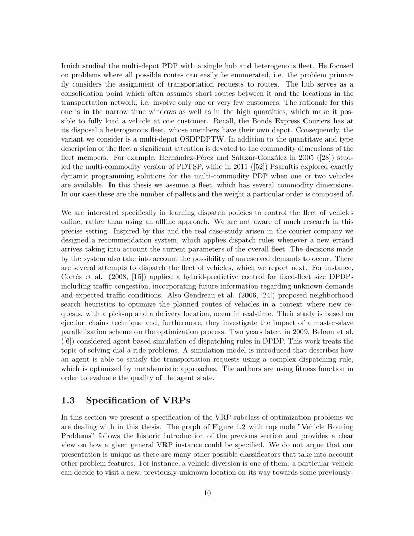
• For each Rj = {rj1 , . . . , rjnj}, there is an associated itinerary Ij = {ij1 , . . . , ijnj

}.Each element ijk is called the timetable associated with the request rjk or requestitinerary is defined as,

ijk =< ajjk , wjjk, bjjk , sjk , e

jjk>,

where ajjk , wjjk

, bjjk , sjk and ejjk are the arrival, waiting, starting, service and departuretimes for the given request.

Similarly, to the home requests we define a timetable at each depot location dj ∈ D. Thatis, a tuple of the form : < cj , 0, cj , 0, pj >, where cj is the time a vehicle is available atdj and pj is the time when it leaves that location. We call such a tuple home itinerary andthe set of those we denote as ID.

Definition 4 : (Routing and Scheduling Plan) A pickup and delivery routing andscheduling plan (PDRSP) is a pair P = (R, I), where R is a routing plan and I is ascheduling plan for it.

From now on we assume that whenever we discuss a PDRSP we know its underlying setof orders. When we work with multiple sets of demands we will explicitly refer to one ifneeded. Our final goal is to construct such a routing and scheduling plan achieving con-venient total costs and managing the fleet in a reasonable way during that day. The nextmeasures address the quality of a fleet schedule. We do not argue that these are all themeasures for evaluting a given plan. Rather than, they were reasonably chosen represent-ing the company interests. From now on in order to avoid a possible confusion with thenotations every time we need a component of a particular request rkj or an itinerary ikj wewill refer to it directly.

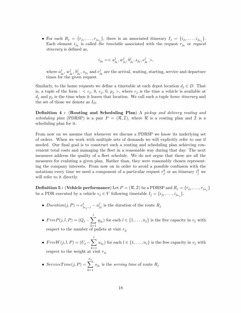
Definition 5 : (Vehicle performance) Let P = (R, I) be a PDRSP andRj = {rj1 , . . . , rjnj}

be a PDR executed by a vehicle vj ∈ V following timetable Ij = {ij1 , . . . , ijnj}.

• Duration(j, P ) = ejjnj−1− ajj2 is the duration of the route Rj

• FreeP (j, l, P ) = (Qj −l∑

k=1

qjk) for each l ∈ {1, . . . , nj} is the free capacity in vj with

respect to the number of pallets at visit rjl

• FreeW (j, l, P ) = (Uj −l∑

k=1

ujk) for each l ∈ {1, . . . , nj} is the free capacity in vj with

respect to the weight at visit rjl

• ServiceT ime(j, P ) =

nj∑k=1

sjk is the serving time of route Rj

18

• WaitingT ime(j, P ) =

nj∑k=1

wjjk

is the waiting time of route Rj

• Lateness(j, P ) =

nj∑k=1

ljjk is the total lateness of route Rj , where ljjk = bjjk − tkl , if

bjjk > tkl or 0, otherwise, is the lateness at visit rjk by vehicle vj

• TravelT ime(j, P ) =

nj−1∑k=1

tjk,k+1 is the total travel time of route Rj

• ExecutionT ime(j, P ) = TravelT ime(j, P )+WaitingT ime(j, P )+ServiceT ime(j, P )is the total execution time of route Rj

• Unsat(j, P ) =

nj∑k=1

penalty(rjk) is the number of unsatisfied customers along Rj , where

penalty(rjk) = 1, if ljjk > 0, and 0, otherwise

The best profit of Rj in terms of serviced clients and execution time could be achieved if wemaximize nj and minimize ExecutionT ime(j, P ), and Lateness(j, P ) possibly satisfyingall hard and soft constraints. As for each request rjk ∈ Rj , sjk is fixed at the locationlk, then ServiceT ime(j, P ) will be fixed for nj requests. Moreover, under the assump-tion that the fleet of vehicles are moving with constant velocity on the road, we have thatTravelT ime(j, P ) is also fixed for a given route. Hence, for a fixed number of customersalong Rj , we can minimize ExecutionT ime(j, P ) only if we minimize WaitingT ime(j, P ).In addition, minimizing Lateness(j, P ) will maximize the customer satisfaction, i.e. max-imize the number of on-time deliveries. Despite the vehicle measures above, one is moreinterested in overall fleet performance or in the quality of work a particular vehicle typeproduces throughout the day. The former gives a possibility to evaluate the entire fleetschedule, while the latter observes more the road behaviour of a particular subset of thefleet.

Definition 6 : (Fleet performance) Let V = {v1, . . . , vm} be the fleet of vehicles,O = {o1, . . . , on} be a set of transportantion orders, and P = (R, I) a PDRSP for managingO by V . Then we define the following features related with this plan :

• ServiceT ime(P ) =m∑j=1

Service(j, P ) is the service time of plan P

• WaitingT ime(P ) =

m∑j=1

Waiting(j, P ) is the waiting time of plan P

• Lateness(P ) =m∑j=1

Lateness(j, P ) is the lateness of plan P

19

• TravelT ime(P ) =

m∑j=1

Travel(j, P ) is the travel time of plan P , i.e. the total travel

time of the fleet

• ExecutionT ime(P ) = TravelT ime(P ) +WaitingT ime(P ) + ServiceT ime(P ) is thetotal execution time of plan P

• Unsat(P ) =m∑j=1

Unsat(j, P ) is the total number of unsatisfied customers in P

• Active(P ) = {Rj | Execution(j, P ) 6= 0} is the set of active vehicles in P

Definition 7 : (Type performance) Let O = {o1, . . . , on} be a set of transportantionorders and V = {v1, . . . , vm} the fleet of vehicles. If T is a vehicle type, then by V T ={vj | vj ∈ V and it is of type T} we denote the set of vehicles of type T . Furthermore, letP = (R, I) be a PDRSP. Then the pair P T = (RT , IT ) represents a PDRSP for V T , wherethe sets RT = {Rj | Rj ∈ R and vj ∈ V is of type T} and IT = {Ij | vj is of type T} are,respectively, the routes performed only by vehicles of that type and their itineraries.

• nT =

|RT |∑j=1

(nj − 2) is the total number of serviced locations by the vehicles of that

type where nj is the number of visits in Rj ∈ RT

• ActiveTR =

|RT |∑j=1

(Service(j, P T ) + Travel(j, P T )) is the time of active performance of

the vehicles from V T

• nTj = nT

2∗|Active(PT )| is the average number of serviced orders per driver of a vehicle

from V T

• AverageDur(P T ) =

|RT |∑j=1

Duration(j, P T )

|RT | is the average schedule duration per vehicle

from V T .

2.2 The Basic VRP

In this section we formulate the core of our problem as a linear integer program. First wedefine three integer variables, two of which serve as order and vehicle indicators and thethird represents the current vehicle freight. In the next, we assume that the sets of indicesfor the depot and customer locations and disjoint. For each vj ∈ V and ri ∈ RO, let xij = 1if and only if the request ri is assigned to vehicle vj . Secondly, the variable yi1i2j = 1 if andonly if the vehicle vj travels between the customers requested ri1 and ri2 , both belonging

20

to RO. Lastly, the variable zcij stores the cummulative load for the commodity c ∈ {q, u}carried by vehicle vj , visiting location li of request ri ∈ RO. It accepts only natural values aswe consider a natural number assigned to each commodity. In each time instant this valueshould be less or equal than the maximum allowed for the particular commodity in vehiclevj . As the only locations where a vehicle could change its capacities are the customer ones,which belong to its route, the value of zcij will increase after visiting a pick-up location andit will decrease when service at a delivery location is performed. Next, we define the VRPproblem in terms of integer constraints using the variables we defined as follows:

1. ∀ri ∈ RO.m∑j=1

xij = 1

2. ∀ri ∈ RO.

m∑j=1

∑rk∈RO

yikj = 1

3. ∀vj ∈ V with home request rj ∈ RD.∑

ri∈RO

yjij = 1

4. ∀vj ∈ V with home request rj ∈ RD.∑

ri∈RO

yijj = 1

5. ∀ri ∈ RO.∀vj ∈ V .∑

rk1∈RO

yk1ij −∑

rk2∈RO

yik2j = 0

6. ∀ri ∈ RO.∀vj ∈ V .∑

rk∈RO

yikj ∗Qj ≥ zqij + qi and∑

rk∈RO

yikj ∗ Uj ≥ zuij + ui

7. ∀ri1 , ri2 ∈ RO ∪RD. ∀vj ∈ V . yi1i2j = 1 ⇒ zqi1j + qi2 = zqi2j and zui1j + ui2 = zui2j8. ∀ri ∈ RO.∀vj ∈ V with home request rj ∈ RD. yjij = 1 ⇒ zqij = 0 and zuij = 0

9. ∀ri ∈ RO.∀vj ∈ V with home request rj ∈ RD. yijj = 1 ⇒ zqjj = 0 and zujj = 0

10. ∀ri ∈ RO.∀vj ∈ V . zqij ≥ 0 and zuij ≥ 0

Table 2.1: VRP constraints.

The first constraint imposes that each transportation request is assigned to exactly onevehicle. Recall, that we do not consider a possibility of transferring packages between dif-ferent vehicles at any location. Hence, an order which has been picked up by one driverhas to be delivered by the same vehicle. The second constraint expresses that each requestin RO is serviced exactly once by exactly one vehicle. The next limitation imposes thateach vehicle departs from its home location (services its home request) towards exactly onecustomer location. Similarly, the vehicle arrives at its home from exactly one customerlocation. The following requirement, sometimes called equilibrium condition, imposes thatwhenever a vehicle arrives at a customer location to perform services, it also must departfrom it. Constraint 6 assures that when visiting a new customer, the corresponding vehiclehas enough capacity to accommodate her needs. The next constraint tells us how to calcu-late the current vehicle load when travelling from one location to another. Also it says thaton its way between any two consecutive visits, a vehicle does not change its capacities exceptat the customer locations associated with these visits. The reason for that is because wedo not allow a cross-utilization amongst fleet members and we do not have store locationsanywhere on the map. Recall, that the amount of load has positive and negative values for

21

the pick-up and the delivery locations, respectively. Next, constraints 8 and 9 impose thateach vehicle depart from and arrive at its depot empty and the last constraint keeps thevalues of the current cummulative commodities non-negative.

2.3 Paired Customers and Time Windows

Following the basic constraints in the previous section, we introduce constraints to imposethat each order is paired (comprised of pick-up and delivery requests). Hence, our locationsare connected and under our assumptions such places should be visited by the same vehicle.A natural precedence constraint is presented and discussed. In addition, each request hasits own time preferences, i.e. time window within which the service at a particular locationshould take place. The earliest such time is a hard constraint as we assume that the packageis not ready before that time. Consequently, if a vehicle arrives earlier than this time, itshould wait in order to start its services. The latest time for a given location is a softconstraint and it could be violated. We pay a penalty for such a delay, which is taken intoaccount when we consider the objective function.

Next, we proceed more formally. Let oi = (r1i , r

2i ) ∈ O be an order. Let r1

i be at location

l1i and r2i at location l2i . In addition, let [ti,1e , ti,1l ] and [ti,2e , ti,2l ] be the time windows related

to these locations. Let the demand oi to be assigned to vehicle vj ∈ V and let Ij ∈ I beits itinerary in plan P = (R, I). Futhermore, let pj be the departure time for that vehicle.Thus, in addition to constraints 1. - 10., the following constraints should also be satisfied.

11. ∀oi ∈ O∀vj ∈ V . xi1j = 1⇔ xi2j = 1

12. ∀oi ∈ O∀vj ∈ V . xi1j + xi2j = 2⇒ djji1≤ djji2

13. ∀oi ∈ O. ti,1e ≤ ti,1l and ti,2e ≤ ti,2l14. ∀ri, rk ∈ RO. ∀vj ∈ V. yikj = 1⇒ djji + tji,k ≤ d

jjk

15. ∀ri, rk ∈ RO. ∀vj ∈ V. yikj = 1⇒ djji + tji,k = ajjk16. ∀ri, rk ∈ RO. ∀vj ∈ V. yikj = 1⇒ ajji + wj

ji+ sjji = djji

17. ∀rj ∈ RD. dj1 ≥ pj

Table 2.2: Paired and time window constraints.

The initial constraint expresses the fact that r1i is assigned to vehicle vj if and only if r2

i

is also assigned to vj . The second constraint relates both the pick-up and the deliverylocations of order oi. It simply imposes that l1i must be visited before l2i . That is, if oi isassigned to vj , then the departure time at l1i must be less than the one at the correspond-ing delivery location l2i . The next limitation imposes the feasibility of the pick-up and thedelivery time windows. In general the release times at two paired locations could differ, butwe assume that the earliest delivery time is equal to the earliest pick-up time. The nextcondition relates any two consecutive departure times and enforces that a vehicle departsfrom its next location after it has departed from its current location plus the additionaltravel time between these locations. Constraint 15 expresses that once a vehicle departs

22

from a location, it arrives at the next one after the required time units. We assume thatthe vehicle driver does not wait somewhere on his way between the two locations. Theonly place he is allowed to wait is at a customer location whenever he arrives earlier thanthe earliest time for that location. The length of the waiting time window associated witha request ri ∈ RO is wi = tie − ai if ai < tie and 0, otherwise. We assume that in thelatter case, the driver starts serving the client immediately after he arrives, as expressedby constraint 16. In other words, the only time a driver spends at a customer location isequal to the service time needed for the corresponding demand. Within this time the drivercould consult a dispatcher about his next destination and then to head towards it. Thefinal condition simply says that each vehicle departs from its home location at the departuretime associated with that depot.

Costraints 1-17 represent a linear integer program corresponding to the static version of ourproblem. This program models our problem as a PDPTW. However, the addressed problemis dynamic as the client orders arrive unpredictable. Thus, hereafter, we discuss the issuesrelated with the dynamic PDPTW version.

2.4 Switching to a Dynamic Setting

In this section we discuss the issues related to the problem dynamics. First, we deal withthe so called one-to-one PDPTW. In other words we have a fleet of vehicles that leaveempty their home locations, serve a particular number of demands and travel empty backto their depots at the end of their job. Each order has a given commodity, which is to beserviced between an origin and a destination. As the time goes by along a working day,the amount of known information revealed to the decision maker is getting larger. Thisknowledge is updated each time a set of new orders arrives, at which moment each vehicleis either moving towards a customer, serving a customer or waiting at a location in orderto start service. In a real-time setting the system should make a decision for each vehiclein the plan, to wait or to go, and for the new order, to accept or to reject it. Following thecompany policy, the system must accept each order, even though it cannot be immediatelyassigned to a vehicle. A decision to assign the order to a given vehicle is made, wheneverthe system evaluates where it can be included. Such an update of the current plan shouldbe based on features of the current pickup and delivery routing and scheduling plan as wellas on the characteristics of the new obligations. In the literature, many approaches haveinvestigated different short-term and long-term features such as the current makespan, i.e.the time the last client is serviced, total latency, i.e. the sum of the completion times forall routes in the current plan, total distance traveled by the vehicles, degree of dynamism,number of the late orders, number of after shift vehicles and many others.

On the other hand, in the process of decision making, predictions can be made on thebasis of historical data. A predicted model of the environment can be useful in severalways. Based on the arrival and commodity distributions we can try to predict with a givencertainty where and when a new order will occur and also what will be its commodities.Using this information would help us to define georgraphical zone characteristics such asaverage total workload within a zone for a given time frame, types of vehicles which should

23

operate within a zone and an interval, waiting and buffering strategies related with thevehicle routes, etc. Thus, simulating artificial obligations could be beneficial for vehiclecontrol and could contribute to achieve better objective values at the end of the day.

2.4.1 Time slices

During the daily time horizon the system could make a great number of small non-optimaldecisions. Therefore, the implemeted final schedule may benefit if we reoptimize the currentpickup an delivery routing and scheduling plan from time to time by taking into accountthe revealed new information. In this way the fleet could advance whenever a new decisionneeds to be made. We split the working time horizon based on the notion of time slices,initially proposed by Kilby et al. ([38], 1998). Although they consider only slices of equallength, we also investigate the case of different duration. For each time slice we solve astatic PDPTW and use its suboptimal schedule as a reference in the evaluation phase ofthe conducted experiments. In total, we consider three horizon divisions. Firstly, we rerouteand reschedule the current plan once at the beginning of the working day, i.e. we have onlyone time slice. In this case we know in advance only the orders stated on the previous days.Note that this strategy coincide with the one of not having slices at all and it has receivedsignificant research attention in the last years. The second division is based on the definitionof time zones. The distribution of the new arrivals can be used for setting the boundariesof such time periods along the day. Then, the plan will be reoptimized before each timezone. This division is motivated by the past data statistics we studied. The third splittingis based on fixed-time-span intervals, i.e. intervals of equal duration. Lastly, we mentiona possibility of rescheduling every time a new event happens. However, to reoptimize allvehicle routes whenever a client has been serviced or a new order has arrived is not realisticin problems with a high degree of dynamism, i.e. if the orders arrive within a time interval,significantly smaller than the time needed for doing any adequate global update (as in thecase with companies such as Bonds Express). Table 2.3 contains the number nts of slicesin each setting and the motivation behind them.

# nts Motivation Slice length

1. 1 paper case fixed

2. 5 arrival distribution variable

3. 7 uniform working time fixed

Table 2.3: Time slices scenarios.

2.4.2 Prediction model

In what follows, we discuss benefits of considering a prediction model. In the literature thereare some attemps to exploit past data in order to anticipate the future demands ([32, 55]).Such a model aims helping to predict where and when possible demands will occur. Forthis purpose we split the time horizon in one-hour intervals. From one interval to the nextthe value of the process increases by the number of the orders arrived within this particularinterval. Therefore, we can view this process as a stochastic counting process. In general,

24

there are two types of counting processes with respect to the arrival rate. One with aconstant increments or homogenous and one that experiences different arrival numbers, i.e.non-homogenous. Moreover, a counting process can be classified with respect to the timehorizon domain. If the domain is discrete, we call the process discrete and countinuous,otherwise. Each discrete counting process can be divided into several subgroups, accord-ing to the distribution of the interarrival time, i.e. the distribution of the time betweeneach pair of consecutive process values. From this perspective, a process can be clasifiedas periodic or aperiodic. The latter type is specialized even further following the specificdistribution mass function. For instance, a Poisson counting process has an exponentialinterarrival distribution (see [49]).

n

t

N(t1)

N(t2)

N(t3)

N(t4)

N(t5)

t1 t2 t3 t4 t5. . .

0

Figure 2.1: Non-homogenous and periodic counting process.

The distribution of the number of arrivals at the system can be approximated by a countingprocess. Figure 2.1 depicts a general graph of a non-homogenous, periodic counting process.We used an instance of it to collect various statistics for the different time intervals (seeSection 4.2.5). For each of them we studied the distributions of the order features (seeSection 2.1) based on past data and then used the statistics to generate one hundred datasetsof orders. Their goal is to simulate fleet activity and in this manner to allocate the vehiclesin positions, which are better for handling the occurrence of possible unreserved demands.

2.5 Objective Function

In this section we present the objective function of our problem, aiming at total minimizingthe final total costs spent throughout a day for running the fleet. The costs are made upfrom the total vehicle running costs, driver wages, penalties for late services as well as extracosts for after-shift work. Since we assume heterogenous fleet of vehicles, the cost the com-pany pays to have different vehicle types on the road is described in Table 1.1. In addition,

25

the driver wage has a constant value 1, which is based on hourly basis. We proceed moreformally by presenting the request graph. A structure on top of which the desired objectiveis defined.

Definition 8 : (Request graph) Let RO ∪ RD be the request source of our problem.Then, a request graph GO is a pair (NO, EO), where (1) ri ∈ NO if and only if ri ∈ RO ∪RD

and (2) (ri, rj) ∈ E if and only if ri, rj ∈ RO ∪RD.

The request graph is just a network of all the order and home requests. Its nodes containthe information about the individual requests, while its edges relate them. Note that it isa fully connected, directed multi-graph and it imposes no restrictions either on the fleet oron their routes. Therefore, we relate the PDR of a given vehicle with a route in the requestgraph.

Definition 9 : (Vehicle Graph Route) Let V = {v1, . . . , vm} be the considered fleet,GO = (NO, EO) the request graph, and Rj = {rj1 , . . . , rjnj

} the PDR for vehicle vj ∈ Vaccording to the PDRSP P . A vehicle graph route RGO

j corresponding to Rj is the orderedset {(rjm , rjm+1) | m ∈ [1, nj − 1]}.

Note that for each vehicle vj ∈ V the vehicle graph route RGOj is a specific subgraph of the

request graph GO. Also as the vehicles service disjoint request subsets of RO, it follows thatthe vehicle graph routes represent disjoint subgraphs in GO. The latter does not prevent tohave a common request location in more than one vehicle graph route and which is visitedmore than one time. Furthermore, note that for each vehicle graph route RGO

j there is anitinerary Ij ∈ I associated with it.

In what follows we define the costs the company pays when a vehicle traversing its graphroute. Let V = {v1, . . . , vm} be the fleet and for each vehicle vj , let c′j be the price to havevj on the road and c′′j the driver’s wage. Also recall that for any two locations ls, lk ∈ L∪Dwe denote by ds,k the distance and by tjs,k the travel time between them.

Definition 10 : (Edge cost) Let RGOj be the vehicle graph route for the vehicle vj ∈ V

and Ij = {ij1 , . . . , ijnj} be its itinerary. Then for each edge (rjs , rjs+1) ∈ RGO

j the cost fortraversing it by vj is given with the expression :

cjsjs+1 = c′j ∗ djs,js+1 + c′′j ∗ (tjjs,js+1+ wj

js+1+ sjs+1) + pjjs+1

,

where (1) wjjs+1

, sjs+1 ∈ ijs+1 are the waiting and service times at the location of rjs+1 and

(2) pjjs+1is the penalty cost for the lateness at this location, if incurred. Note that a penalty

at the last location means for some after-shift work. However, we do not differentiate it fromany other penalty and we calculate all of them the same way. The latter can be done takinginto account how urgent is the particular request. Nevertheless, we describe this concept inthe next chapter when we discuss the cost-forming factors observed by a dispatching rule

1According to the NICTA internal report from September 6, 2011.

26

when evaluating where the new orders are to be inserted.

Definition 11 : (Route cost) Let RGOj be the vehicle graph route for the vehicle vj ∈ V

and Ij = {ij1 , . . . , ijnj} be its itinerary. Then the cost vj needs to execute the entire graph

route RGOj is the following :

cj =∑

(rjs ,rjs+1)∈RGO

j

cjsjs+1

Definition 12 : (Schedule cost) Given a plan P = (R, I) ∈ P from a set of plans formanaging the fleet V = {v1, . . . , vm}, the objective function f : P → R, which takes a planand returns a real number is given by the next expression where ej = (rjs , rjs+1):

f(P ) =m∑j=1

∑ej∈R

GOj

cjsjs+1 =

m∑j=1

∑ej∈R

GOj

(c′j ∗ djsjs+1 + c′′j ∗ (tjjsjs+1+ wj

js+1+ sjs+1) + pjjs+1

) =

m∑j=1

∑ej∈R

GOj

c′j ∗ djsjs+1 +m∑j=1

∑ej∈R

GOj

c′′j ∗ (tjjsjs+1+ wj

js+1+ sjs+1) +

m∑j=1

∑ej∈R

GOj

pjjs+1

The first term in the objective function f(P ) expresses the cost the company pays to runthe entire fleet V according to P , the second represents the accummulated cost for thedrivers’ wages and the third accounts for the overall penalties for the late services. We mayalso express f(P ) by :

f(P ) =m∑j=1

∑ej∈R

GOj

c′j ∗ djsjs+1 +m∑j=1

∑ej∈R

GOj

c′′j ∗ tjjsjs+1

+m∑j=1

∑ej∈R

GOj

c′′j ∗ wjjs+1

+

m∑j=1

∑ej∈R

GOj

c′′j ∗ sjs+1 +m∑j=1

∑ej∈R

GOj

pjjs+1,

where there are distinct terms for the total travel, total waiting and total service costsrelated with the plan P . All the cost components may serve as meaningfull indicators ofthe quality of a given plan. In general, one would be interested in minimizing the penaltyterm in the objective function and possibly to have control over the waiting term (it mightbe beneficial to wait some time at a customer location, but not too long). Finally, wepresent the objective function in terms of the integer variables we introduced previously.Recall, xij = 1 if and only if the i-th request from RO is assigned to vehicle vj ∈ V , andyi1i2j = 1 if and only if vehicle vj ∈ V elapses the distance between locations li1 and li2from L ∪D.

f(P ) =2∗n∑i=1

m∑j=1

xij

2∗n∑k=1

(yikj ∗ cik)

27

2.6 NP-hardness

Here, we briefly discuss the theoretical complexity of the problem in hand. The Pickupand Delivery Problem (PDP) is a kind of Vehicle Routing Problem (VRP), a variant ofthe Travelling Salesman Problem (TSP), which is well-known to be an NP-hard problem.These problems are particularly expensive as the exact algorithms solving them require, ingeneral, exponential time. We do not show a detailed proof of NP-hardness for TSP (see[29, 36]), but we underline the major issues when is to be reduced to our problem.

In the classical TSP there is a set of cities, travel cost for each pair of them and a salesman.The goal is to construct such a visiting assingment of the salesman through all the citiessuch that the overall travel expense does not exceed a predetermined value. This problemis reducible to the task of finding a Hamiltonian cycle in the graph of locations. Therefore,as a single-vehicle VRP is reducible to the classical TSP, it means that a single-vehiclePDP does so as well. However, when the fleet includes many vehicles another problememerges related to the vehicle assignments, i.e. how to partition the set of cities (clients)with respect to the number of ”salesmen”, so that for each vehicle and its respective set ofcities a TSP algorithm is applied. Hence, multi-vehicle routing problem is harder that thesingle-vehicle one as two phases can be distinguished : (1) building vehicle assignments orpartition the set of all customers and assign them to the vehicles and (2) for each vehicleapply TSP algorithm to optimize its route. We already discuss that problem 2 is NP-hard,however, this time we have multiple such problems. The problem 1 is also NP-hard becausethere is an exponential number of partitions for the set of all locations. Thus, we have anexponential number of possible vehicle assignments. Although, we do not give precise proofof the complexity, we believe that the problem in hand is at least as hard as a problem fromNP TSP , i.e. problems which are solvable by a non-deterministic Turing machine in a timeproportional to the one needed for solving a TSP instance. Recall, the VRP solver Indigo2.0. has a two-phased architecture. The first one is related to finding a reasonable vehicleassignment (problem 1 above) and during the second one the oracle tries to optimize all theroutes for a certain number of local search iterations (problems of type 2).

28

Chapter 3

Simple Dispatch Heuristics

Making a decision can be vital.by Martin Aleksandrov

This chapter addresses the heuristics we implemented and tested within our framework. Itstarts with a short introduction of the general circumstances under which the dispatchershave to make a decision about acceptance or rejection of a new arrival. It might be difficultfor them to be aware of all the current parameters of the fleet and the environment in orderto perform the best decisions. The online heuristic algorithms presented here, intend tohelp them in their daily work.

In the first section we introduce several notions related with a current pickup and deliveryrouting and scheduling plan. Then we discuss cost-forming issues that must be taken intoaccount by each online heuristic decision.

Next sections cover the decision-making heuristics and explain the schedule and orderfeatures they take into account. We formalize and discuss the constraints they impose.Amongst these are Minimum Cost, Balanced, Current Orders, Shift Profitability,Geographical Closeness, Minimize Vehicles, Immediate Cost and Random heuris-tics. We partly talk about their correctness and worst-case complexity in the main bodyand leave the rest in the Appendix. At the end of this chapter we summarize the maincomputational results.

29

3.1 General Assumptions

An inquiry could be requested either via phone conversation or via company webportal. Inaddition to these dynamic demands there is also a significant number of orders stated onprevious days and the information about them is available in the morning of the workingday. The dynamism of the problem is a consequence of the arrival frequency of previouslyunknown errands. When such a stochastic event occurs, a dispatcher needs to decide onwhich route of which vehicle the new order should be included so that a certain set ofconstraints is satisfied in some optimal way. As they follow a policy aiming to maximizethe number of serviced and satisfied customers, the dispatchers expect that the system willadvice them in a reasonable time. This policy is adopted by the company aiming at loosingno customers. After a dispatcher accepts a given order, he could decide to inform a driverof the recommended vehicle immediately when it is not in a motion or to buffer the newdemand for a while according to a predetermined strategy. The last decision partly dependson the current system response in terms of the immediate versus delayed profit gained byassigning the new demand to that vehicle.

In the considered setting the smallest time interval within which new orders can be dis-tinguished is one minute (we do not distinguish between orders, which arrive in differentseconds within a particular minute), so the time can be considered as discretized. This issuealso has other benefits, which we are going to discuss in chapter 5 where we describe thelearning mechanism. We proceed more formally by introducing several notations, which weare going to use in the following sections.

Demands Let t be the moment (minute), in which new demands arrive at the system.The set Lt contains all the customer locations known by this time instant. Also let the setof all previously scheduled transportation orders be Ot = {o1, . . . , on} and the set of newarrivals St = {s1, . . . , sk}. Each order sk contains information about two requests, denotedas s1

k and s2k. In addition, qk and uk are the commodity values associated with sk for the

number of pallets and its weight, respectively. They are positive for s1k and negative for s2

k.In other words, the positive commodities are to be transported from l1k to l2k, which are therespective locations.

Time windows Also there are time windows at each location, which express customerconvenience. Let [tj,1e , tj,1l ] be the one at l1j and [tj,2e , tj,2l ] at l2j . Recall, we assume that

tj,2e = tj,1e .

Fleet The new transportation orders are assigned to vehicles of the company fleet V ={v1, . . . , vm}. Each fleet member vj has given maximal capacities, Qj and Uj , and its owndepot, located at dj ∈ D (the set of depot locations). Vehicle availability is based on thehistorical data and it takes into account the driver maximum shift length of eight hoursstated in their contracts. We assume three vehicle shifts, i.e. 5 a.m. - 13 p.m., 9 a.m. - 15p.m. and 13 p.m. - 19 p.m..

30

Plans Let P t = (Rt, It) be the PDRSP in the time instant t. That is, each vehicle vj ∈ Vis assigned to exactly one route Rt

j according to Rt following the itinerary Itj ∈ It. Recall,Rt

j = {rj1 , . . . , rjnj} is an ordered set of requests, starting and ending with the respective

home request (rj1 ≡ rjnj≡ rj ∈ RD), and each intermediate demand rjk ∈ Rt

j corresponds

to an order request from ROt (the set of the assigned requests so far), either a pick-up or adelivery, which is located at ljk ∈ L.

Based on the notations above we will define some notions related with them. A vehicleroute Rt

j is called empty if nj = 2, i.e. there are no other requests assigned to it except thehome ones. On the other hand, a non-empty route contains an even number of customerdemands as we consider a PDP.

With respect to the dynamic moment t and the plan P t we can distinguish several vehiclestates. If a vehicle has finished its job, it is not available anymore that day narrowingdefault availability time window. Here, we assume a vehicle has finished its work if it hasleft the last customer on its route according to P t. Other vehicle state is when the driver isheading towards his next destination, in which case the vehicle cannot be diverted. In timet a vehicle can also be serving a client or waiting at a customer location in order to startits duties. In both cases the driver can be consulted by a dispatcher about his next jobs.Also a vehicle may have no assigned requests at time t and be available waiting at home.Such a vehicle has a currently empty route and if it is profitable enough a driver can becontracted for the rest of the respective availability window. Such vehicle is considered as acandidate for a new order if this is to be serviced after the beginning of the driver shift time.

Regarding the vehicle states we can distingusih several types of assigned visiting sequences.If vj has executed its route by the time t, Rt

j is infeasible with respect to t. Also Rj can beinfeasible with respect to t if vj starts its shift after t and there is no new order sk ∈ St tobe serviced after that time. Otherwise, Rt

j is a possible route regarding t. Next, if vj cannotmeet the capacity constraints with respect an order sk ∈ St the route Rt

j is infeasible withrespect to sk. Hence, Rt

j is a possible route, whenever it is feasible with respect to t and toan order from St. When the system makes a decision where to include a new demand it hasto take into consideration both the non-empty and empty feasible routes. Also, as we havea paired variant of VRP, for each sk ∈ St a decision should be made for both s1

k and s2k.

The paired constraints relating these requests must be satisfied, i.e. both s1k and s2

k must beserviced by the same vehicle vj and l1k must be visited before l2k. Thus, the inclusion of skhas to be done in a sequence. We call a gap each pair of consecutive visits along a vehicleroute. Thus, each heuristic must evaluate all gaps within the possible routes in the currentplan. A gap is a possible place for accommodating a new demand if it satisfies a collection ofconstraints imposed by a heuristic. When given an order sk ∈ St each heuristic computes allpossible gaps along all possible routes together with their additional costs. It also takes intoaccount the vehicle states according to P t. Then as candidates for accommodating the neworder are considered only those pairs of spots, which have as first component a ”pick-up”gap and as the second one a ”delivery” gap. Finally, the pair of gaps with minimal totalcost is selected. In this sense, apart from only considering order and schedule features, theheuristics try to minimize the local extra expenses.

31

3.1.1 Possible routes

As discussed in the previous paragraph whenever new orders arrive we need to determinewhich routes possibly can accommodate them. The last can be done if we first determinethe possible routes with respect to the arriving moment.

Let t be the considered instant, in which order sk ∈ St arrives. Also let P t = (Rt, It) bethe current plan. Then a route Rt

j = {rj1 , . . . , rjnj} from Rt is a possible candidate with

respect to t if it satisfies the following constraints:

F 1. djjnj−1≥ max(t, tk,1e )

F 2. djj1 ≤ max(t, tk,1l )

Table 3.1: Route constraints : regarding the arrival moment.

Constraint F 1. requires that vehicle vj is still executing its route, i.e. its departure time of

the last customer is at least the maximum of t and tk,1e . Otherwise, the vehicle either willtravel on its way to its depot or it will be already at home. The second constraint imposesthat vj should have started executing its duties by the maximum of t and tk,1l . In general,

we have t ≤ tk,1l . However, to keep generality, we assume that it is possible that tk,1l ≤ twhen a package has been delayed for processing, but it has to be delivered the same day.Then we consider only the moving vehicles as possible candidates for that package. Notethat both constraints restrict the set of all routes P t with respect to [tk,1e , tk,1l ], but there is

a possibility to violate [tk,2e , tk,2l ], albeit at the cost of additional penalties, l2k can be visitedeither in an after-shift time or it can imply possible late services at some of the successivelocations.

3.1.2 Capacity constraints

To consider a route as a possible candidate to accommodate the new demand, it must meeta set of constraints regarding the capacity dimensions of the vehicle and the new order. Aswe consider only two commodities, i.e. number of pallets and weight, we have only twoconstraints.

Let t be the moment, in which order sk ∈ St arrives. Let its commodity dimensions be qkand uk for the number of pallets and its weight, respectively. Also let P t = (Rt, It) be thecurrent PDRSP in. Then a route Rt

j = {rj1, . . . , rjnj} from Rt is a possible candidate with

respect to sj if it satisfies the following constraints:

C 1. qk ≤ Qj

C 2. uk ≤ Uj

Table 3.2: Route constraints : regarding the new order capacities.

32

3.1.3 Additional travel costs

There might be extra expenses when a vehicle is diverted from its current state in order toservice a new order. The heuristics should compute such costs and we discuss the assump-tions made when calculate them.

Let us consider a route Rtj = {rj1, . . . , rjnj

} executed by vehicle vj ∈ V running with

average velocity of mj . Let further sk = (r1k, r

2k) ∈ St be a new order and let rjs and rjs+1

be the visits between which we want to compute the extra costs for serving a request rvkbeing either r1

k or r2k. In addition, let [tk,ve , tk,vl ] be its time window. Recall, c′j is the cost

the company pays per kilometer for having vj on the road and with c′′j is denoted the wage

of that vehicle driver. Also, recall, that sjk is the service time needed for rpk. Then the

additional travel time needed by vj is tjk = tjjs,k + tjk,js+1− tjjs,js+1

. Furthermore let wjk

be the waiting time at the new location lpk defined as follows : wjk = tk,pe − (djjs + tjs,k) if

djjs + tjs,k < tk,pe and 0, otherwise. Thus, the extra travel plus driver costs are given by theexpression :

cji = c′j ∗ (tjk ∗mj) + c′′j ∗ (tjk + sjk + wjk) + pjk.

The first term is the cost the company pays for the additional travel distance and the secondrepresents the extra driver wage, including waiting and service times at the new location.The last term is the penalty incurred in case of delay.

3.1.4 Time window urgency

The travel costs are not the only costs related with the new service. Visiting the new lo-cations can imply late services at some of the successive visits, which lead to additionalundesired costs. We calculate these costs under several assumptions, which we describenext on.

Let, again, t be the moment when sk ∈ St arrives and let rpk be one of its subdemands. Also,

let [tk,pe , tk,pl ] be the time window at lpk. We assume that the length of that time windowreflects the customer urgency about receiving his packages with respect to the moment theyare demanded. Let vj ∈ V is assigned to that request and it arrives at lpk at time T > tk,pl .

Thus, we define a measure of lateness as Ljp = T−tk,pe

tk,pl −tk,pe

to express the delay at lpk by vj .

It has a value greater than 1 and it aims to capture the urgent need of the customers toreceive their deliveries. For instance, a delay of 10 minutes in a time window of 30 minuteshas L = 40

30 ≈ 1.33, whereas the same delay in a time window of 5 hours leads to a value ofL = 310

300 ≈ 1.03

In addition to the lateness measure we also need to determine the costs related to a particu-lar delay. The last is simply the serving cost according to the current scheduling plan. Moreformally, let vj is late at lh and let according to the current plan P t the cost for serving the

parcels at lh be cjh. Hence, the penalty we assign to lh is pjh = Ljh ∗ c

jh.

33

An interesting case is when a vehicle needs an extra time after its shift. In that scenario,each driver is paid according to special regulations, which are not in the scope of this thesis.Thus, we assume he is awarded the same hourly rate stated in his contract when workingunder standart conditions. Hence, the after-work delay is captured as a regular delay atany of the locations. However, in this case the lateness is regarding the depot time window,which is exactly the shift time of the driver.

3.1.5 Distance measures

Both the regular travel costs and the penalties discussed above are time-dependent. How-ever, the real continuious time might be sometimes inappropriate measure of the vehicleperformance due to the possible waiting times at some locations or rare and imperfect com-munication between the drivers and the dispatchers, for instance. Thus, a discretized andqualified measure need to be used when we evaluate the vehicle performance between clients.Such measures are usually the distance measures related to the concrete VRP. Ideally, itwould be a situation, in which we use a Geographical Information System (GIS) to retrievethe real-time road distances between any two geographical points in the considered area.In this work we do not consider such a scenario due to the absence of a proper GIS module.However, we use the Vincenty distance as a good approximation measure of the straight linebetween any two locations on the Earth. Notice that each road-based distance between twopoints can be represented as a finite linear combination of multiple Vincenty-based distances.

The depot and customer pickup and delivery locations are generated uniformly and inde-pendently of each other, and they are specified by their latitude and longitude coordinates.Let lj , lk ∈ L ∪ D be two locations. Then the Vincenty distance is realized via the func-tion VincentyDistance(lj , lk), which is used hereafter by the implemented heuristic algo-rithms. As not being a major topic of our scope we leave the opportunity to the inquisitivereader to read more about the formulae in [56].

34

3.2 Heuristics

In the following sections we describe the heuristics we realized. Each one begins with aninformal description of the considered heuristic and then it introduces the constraints therule imposes during the evaluation. Each rule observes the current PDRSP P t and a neworder sk ∈ St, and it returns a recommendation on where sk should be included. We calleach such decision a suggestion because it just allocates the new loads to a vehicle route.This type of decision allows us to rearrange some of the vehicle loads later on. However,a commitment to an order is a decision after which we cannot change the carrier of thatdemand.

3.2.1 Minimum cost heuristic

Minimum cost heuristic calculates the cost of including the new order between any two con-secutive visits along a route of a possible candidate. In addition, all hard constraints haveto be met, i.e. vehicle capacities and the earliest pickup times of both the new order andthe succesive customer locations. The increase on the objective function is made up of theadditional travel costs for visiting the new locations, the extra expense of a possible waitingand a certain service times at those locations, any additional penalties for late pickups anddeliveries as a result of the incurred vehicle diversion, and possibly a supplementary costfor the extra time needed to make deliveries at the end of the vehicle shift. Finally, theheuristic selects the feasible gap between the visits with minimum extra expenditures.

Let the time instant, in which the new order sk ∈ St arrives be t. Let also P t = (Rt, It)be the current plan and let Rt

j = {rj1 , . . . , rjnj} be a possible route in it run by the vehicle

vj ∈ V . Furthermore, let rt be the current position of vj (either at some location ljs asso-ciated to a visit rjs ∈ Rt

j or at some position between two visits). In addition, let rpk be oneof the two requests constituting the order sk. Then a pair of consecutive visits (rjs , rjs+1)along Rt

j with s ∈ {1, nj − 1} is a possible place where rpk can be inserted if the followingconstraints are obeyed:

M 1. ∀l ≥ s+ 1.qk ≤ Qj −l∑

h=1

qjh

M 2. ∀l ≥ s+ 1.uk ≤ Uj −l∑

h=1

ujh

M 3. djjs + tjjs,p ≥ tk,pe

M 4. djjs + tjjs,p ≤ tk,pl

M 5. djp + tjp,js+1≥ tjs+1

e

M 6. tk,pe′ ≤ tk,pl′ ,

where tk,pe′ = max(tk,pe , tjse + tjjsp) and tk,pl′ = min(tk,pl , tjs+1

l − tjpjs+1)

Table 3.3: Minimum Cost constraints.

35

The first two constraints guarantee that the decision to include rpk between rjs and rjs+1

will not result in a violation of the vehicle maximal capacities, namely the number of palletsand the weight. The next pair of conditions imposes that vj should arrive at the location lkiof rki no earlier than the time the package is ready and no later than the latest preference ofthat customer. The latter condition is required only for the new demand. All the remainingvisits can be assigned a positive delay at their locations. In addition, after we leave thisnew location we must arrive at the next scheduled visit, i.e. rjs+1 , later than its earliestpick-up time in order to avoid waiting there. The last constraint, M 6., checks whether thetime window at the location of rki is feasible with respect to the gap (rjs , rjs+1).

Implementation

The new order sk is composed of a pickup r1k and a delivery r2

k requests. Thus, a fesiblegap needs to be selected for both subdemands. In addition, both the pickup and the de-livery locations of the new order needs to be placed somewhere after rt and the pickuplocation should precede the delivery one. Let vehicle vj be on its way to rjs or already atljs . Moreover, let F 1

j = {(p1, q1) | ∃l ≥ s.(p1, q1) = (rjl , rjl+1) is possible place for r1

k} and

F 2j = {(p2, q2) | ∃l ≥ s.(p2, q2) = (rjl , rjl+1

) is possible place for r2k} be the sets of possible

gaps along Rtj for the pick-up and the delivery requests, respectively. We are interested in

those (p1, q1) and (p2, q2) such that p2 occurs after p1 or p2 = p1. Among these, the systemselects the one with minimum combined cost increase.

The algorithm starts with the initialization of several variables, where it will store the fea-sible spots and their costs, respectively. Then it determines the set of possible routes Rt

pos..In this step we check for each route Rt

j ∈ Rt whether it satisfies the constraints F 1., F 2.,C 1. and C 2. The next cycle collects all the possible gaps for each possible route Rt

j in the

sets F 1j and F 2

j according to the constraints M 1. - M 6. and at the end of each iteration

it follows an update of the global variables F 1 and F 2. After this, set F 1 contains the setsof all possible gaps for the pickup request, and similarly, for set F 2, regarding the delivery.Next, for each route in Rt

pos. we select a possible pickup gap and we summed up its costtogether with the cost for each delivery gap from F 2. If this calculated cost is less thanthe current minimal cost, the algorithms updates its value and the currently best locations,where the new subdemands could be included.

The supplementary costs for inserting the request rpk between the visits rjs and rjs+1 arecalculated by the function IncreaseCost(rjs , rjs+1 , r

pk, R

tj), which takes into account the

cost for the additional travel time to the location lpk, the costs related with a possible

waiting wjp and a certain service sjp at that location and the penalties for the possibly

implied future lateness at previously planned locations, and in particular the extra ex-penditures for after-shift work. The IncreaseCost() function calls the distance methodVincentyDistance(r1, r2), which returns the geodesic distance between the locations ofthe requests r1 and r2. The cost is then computed as described in Section 3.1.3. In thealgorithm the value of bjjs is the start time at the location associated with the request rjs

by the vehicle vj according to its current schedule Itj , djjs

is the departure time at the same

36

location of the same vehicle and tjsl is the latest time for the request rjs . Also cjjs is the cost

for serving the client at ljs by vj according to P t and the fraction dmj

is the average time,

within which vj elapses the distance d.

Algorithm 3.2.1: MinimumCost(P t, sk)

comment: *The algorithm MinimumCost returns the feasible gaps for sk*

comment: *in a route from Rt with minimal extra cost.*

1. F 1 = ∅, F 2 = ∅, C1 = ∅, C2 = ∅2. min cost = max3. min pickup,min del

4. P tpos. = PossibleRoutes(Rt, t, sk)

5. for Rtj ∈ Rt

pos.

6. F 1j = ∅, F 2

j = ∅, C1j = ∅, C2

j = ∅7. for e = s to nj8. if PossibleGap(rje , rje+1 , r

1k)

9. c1ee+1 = IncreaseCost(rje , rje+1 , r

1k, R

tj)

10. C1j = C1

j ∪ {c1ee+1}

11. F 1j = F 1

j ∪ {(rje , rje+1)}12. if PossibleGap(rje , rje+1 , r

2k)

13. c2ee+1 = IncreaseCost(rje , rje+1 , r

2k, R

tj)

14. C2j = C2

j ∪ {c2ee+1}

15. F 2j = F 2

j ∪ {(rje , rje+1)}16. F 1 = F 1 ∪ F 1

j , F2 = F 2 ∪ F 2

j

17. C1 = C1 ∪ C1j , C

2 = C2 ∪ C2j

18.for Rtj ∈ Rt

pos.

19. for (p1, q1) ∈ F 1j

20. for (p2, q2) ∈ F 2j

21. if p1 ≥ p2

22. cost = c1 + c2

23. if cost ≤ min cost24. min cost = cost25. min pickup = (p1, q1)26. min del = (p2, q2)

27.return ({min pickup,min del})

37

Complexity and correctness

Here we discuss the correctness and the complexity of the algorithms. The heuristic correct-ness depends mostly on the correctness of the methods PossibleRoutes(), PossibleGap()and IncreaseCost(). The first procedure checks whether a route is a ”good” candidatefor the new loads. The last is done with respect to the current plan P t. If it does, thenthe procedure includes it in Rt

pos., otherwise not. The correctness of this method is partlyensured by the fact we have a strong system of inequalities F 1., F 2., C 1. and C 2..The second function checks whether a gap is a possible place according to the conditionsM 1. − 6.. Note that the last two procedures depend on the quality of the Rt. At thebeginning of the working day we start with an optimal schedule for all the predeterminedorders. Such a plan is of high quality and we have to quarantee that applying an heuristic,thereafter, it preserves a collection of some general assumptions.

Algorithm 3.2.2: IncreaseCost(rje , rje+1 , rpk, , R

tj)

comment: *The function computes the extra cost for inserting rpk between the*

comment: *visits rje and rje+1 .*

1. extra cost = 02. dje,p = VincentyDistance(rje , r

pk)

3. dp,je+1 = VincentyDistance(rpk, rje+1)4. dje,je+1 = VincentyDistance(rje , rje+1)5. d = dje,p + dp,je+1 − dje,je+1

6. mj = the average velocity of vj [km/h]7. c′j = the cost the company pays when vj is on the road [$/km]

8. c′′j = the hourly driver wage vj [$/h]

9. extra cost + = d ∗ c′j + dmj∗ c′′j

10.wjp = (tk,pe − djje,p −

dje,pmj

> 0)? tk,pe − djje,p −dje,pmj

: 0

11.sjp = the service time at lpk

12.extra cost + = (wjp + sjp) ∗ c′′j

13.for rje ∈ Rtj ∧ rje is visited after rpk

14. ljje = bjje + dmj− tjel

15. if ljje > 0

16. Ljje

=bjje+ d

mj−tjee

tjel −tjee

17. extra cost + = Ljje∗ cjje

18.return (extra cost)

38

For instance, a vehicle capacity must not be exceeded at any time point or we cannot ac-tuate a vehicle, which has finished its duties or its availability window opens later. Thelatter is ensured by computing the set of possible routes in Rt. The reader can find moredetails about the quality of the initial schedule as discussed in Section 4.3.1. Lastly, thecorrectness of the function IncreaseCost() is guaranteed as the Vincenty measure is apositive one and it satisfies the triangle inequality. This is important as the value of d atline 5. in the algorithm must be greater than or equal to zero. The gaps returned by theMinimumCost() heuristic have their total extra cost minimal. However, note that theremight be a gap for either the pick-up or the delivery requests with lower extra cost. Forinstance, such pairs could have the delivery visit preceding the pick-up one. Also notethat the gaps for the pick-up and the delivery demands could concide. In the latter casethe pick-up request, again, must be visited before the delivery one. Thus, the describedalgorithm produces the minimum insertion cost with respect to sk ∈ St, which is somehowdistributed between the cost for inserting the pickup location and the cost for inserting thedelivery location.

About the complexity of the presented algorithm, we first determine the possible routes inline 4. of the MinimumCost() algorithm. This operation requires time linear to the fleetsize m, i.e. O(m), as checking the constraints F 1., F 2., C 1., C 2. for every route from Rt

and order sk ∈ St requires a constant time. Further, collecting all possible gaps and theircosts (lines 5.− 17.) for both the pickup and the delivery request needs a time proportionalto the maximal number of visits in Rt. Hence, if nmax is the number of visits in the longestroute in Rt, then the complexity of selecting all these spots for a subdemand in the worst-case is O(m ∗ n2

max). For each gap the function PossibleGap() takes O(nmax) because ofconstraints M 1. and M 2.. The calculation of extra costs is done using IncreaseCost()for all ”good” gaps. It requires a worst-case complexity boundary of O(nmax) caused bythe calculation of the penalties along the route, which are the result of the possible vehiclediversion between the considered pair of visits. In lines 18.−27. of the algorithm the minimalextra cost amongst all pairs of gaps satisfying the precedence constraint is computed. Thiscalculation needs O(m ∗n2

max) time in the worst-case scenario. Then the overall complexityaccording to the worst-case scenario is thus O(m ∗ n2

max). Better complexity results areachieved in practice due to the fact that we consider proper parts of any of the routesin Rt

pos. For a fixed route and a fixed visit in it we need to perform a ”goodness” testonly for the successive visits. Also the set of possible routes could have cardinality severaltimes smaller than the power of Rt. Let it be mpos. = | Rt

pos. |. Thus, lines 5. − 17.can be processed in time o(mpos. ∗ nmax), where this time nmax is the maximal number ofvisits in the tail of a route from Rt

pos.. The reason for that is because we start to look fora convenient place from the current position of the corresponding vehicle onwards. Lastobservation is expressed by setting the counter e = s to nj to iterate over parts of theroutes rather than the whole routes. Hence, a rough approximation of the lower complexitybound is o(mpos. ∗ (k ∗ (nmax−1

2 ) + (nmax − k) ∗ (nmax−12 + nmax))), where k ∈ [1, nmax] is

the number of the gaps passed the ”goodness” test along the route with nmax visits. Thus,Θ(m ∗ n2

max) could be given as an overall complexity of the decision-making procedure.

39

3.2.2 Balanced heuristic

The Balanced heuristic aims to distribute the overall workload amongst the vehicles. Firstit computes the set of all vehicles, which are able to accommodate the given order withoutviolating any of the hard (earliest times and vehicle capacity) and soft (latest times) con-straints at the current and the successive visits. If this set is empty then we consider theset of all vehicles that have feasible routes. For every vehicle from this set we compute itsfuture planned work according to the current pickup and delivery routing and schedulingplan. Then the heuristic selects the vehicle with minimum amount of scheduled work andthe new order is inserted in a place along its route with minimal additional costs. An inter-esting case is when more than one vehicle have the same minimum amount of future work.Then the new order should again be included with minimum outlay.

Let the new order sk = (r1k, r

2k) ∈ St arrives at time t and let Rt = {Rt

1, . . . , Rtm} be the set

of open routes in time instant t. Let Rtj = {rj1 , . . . , rjnj

} be a possible route for sk and let

the vehicle assigned to it be vj ∈ V . Furthermore, let the current position of vj be rt. Apair of consecutive visits (rjs , rjs+1) along Rt

j with s ∈ {1, nj − 1} is a possible place for rpk(p = 1, 2) if the following conditions are met:

B 1. ∀l ≥ s+ 1.qk ≤ Qj −l∑

h=1

qjh

B 2. ∀l ≥ s+ 1.uk ≤ Uj −l∑

h=1

ujh

B 3. djjs + tjjs,p ≥ tk,pe

B 4. djjs + tjjs,p ≤ tk,pl

B 5. djp + tjp,js+1≥ tjs+1

e

B 6. djp + tjp,js+1≤ tjs+1

l

B 7. tk,pe′ ≤ tk,pl′ ,

where tk,pe′ = max(tk,pe , tjse + tjjs,p) and tk,pl′ = min(tk,pl , tjs+1

l − tjp,js+1)

Table 3.4: Balanced constraints.

The constraints B 1., B 2. ensure the future load satisfaction as in the MinimumCost()heuristic. The following pair of conditions requires that the hard and soft constraints ofthe new demand are fulfilled. In other words the service must take place within its timepreferences. The same check is performed with respect to the successive scheduled visit, i.e.rjs+1 and the last requirement guarantees the feasibility of the time window at the locationof the new request with respect to the gap between rjs and rjs+1 . Note that satisfying theabove constraints means that if we divert vj to serve rpk it would not cause any late penaltiesor after-shift time onwards. The reason for this is that serving the new packages does notchange the current vehicle schedule Itj . Moreover, in order to assign sk ∈ St to vj , R

tj needs

to have either at least two different ”good” gaps or to have one into which can fit both thepickup and the delivery requests.

40

3.2.3 Current orders heuristic

The aim of this heuristic is to entirely reroute the currently known orders whenever a newdemand arrives at the system. To perform such an update we use the VRP solver Indigo2.0. The process of reordering the orders in the system consists not only to schedule thenew demand into some of the routes, but also to remove already serviced orders. The newschedule must also obeys some additional constraints, which we discuss next. The entireset of currently scheduled orders needs to be split into three sets, i.e. set of serviced, set ofundelivered and set of unserviced customers. The set of serviced customers should not influ-ence future reorderings of the rest transportation requests. Furthermore, for each currentordering assigned to a vehicle a list of undelivered customers will be created. They shouldbe visited by the same vehicle in an order possibly different from the one established in thecurrent schedule. Also the set of unserviced customers will be taken into account when theheuristic creates the new plan with the opportunity of schedule them into routes differentfrom the current ones.

In addition to the heuristic description we explain how Indigo can be used only as a decisionheuristic. Recall, the solver has two-phased architecture. During the first phase the initialroutes are constructed using a simple insertion heuristic (construction phase). Next, theimprovement of this initial solution is performed by means of an heuristic combination oflocal search methods. For instance, for producing the optimal solutions in our experiments,we set a combination of Large Neightbourhood Search heuristic together with SimulatedAnnealing heuristic. In order to use and later on evaluate only the simple insert heuristicprovided by Indigo, every time we apply the CurrentOrders rule we update the currentschedule without using any improvement strategies. In this section we will use the termsPDRSP and solution interchangeably as the result of applying the heuristic will be partiallya new plan rather than just the result of including the new order somewhere along a route.

Next, let the new order sk ∈ St arrives at time t and let P t be the current solution. In thismoment each vehicle vj ∈ V is somewhere along its route, either at its depot or performinga service or travelling towards its next customer. Recall, in the latter case we assume thatthe vehicle is at the next destination. Let in the stated three situations the current vehi-cle position of vj along Rt

j be rjc . Then the following conditions must be met during thererouting update.

The first constraint is an interesting one. It requires that the vehicle has new initial de-parture time and it is the one at the location ljc stated in current solution P t. As usual,the next two constraints quarantee that inserting the new demand within the new route,assuming without loss of generality to be again Rt

j , will not affect in violating the capacityconstraints of any future visits in it. The fourth and the fifth restrictions impose that thenew order, if included, should not cause after-shift working time. Note the we allow vj toarrive at the location of rpk earlier than its earliest pick-up time, in which case it will waitthere. The reason for that is the internally implemented DriveF irst ([43]) waiting strategy(in Indigo), which means that as soon as vehicle finishes its work with one customer, it startheading immediately towards the next one. We also permit to occur a situation where vj

41

C′ 1. ∀vj .djj1 = djjc

C′ 2. ∀l ≥ s+ 1.qk ≤ Qj −l∑

h=1

qjh

C′ 3. ∀l ≥ s+ 1.uk ≤ Uj −l∑

h=1

ujh

C′ 4. djj1 + tjj1,p ≤ djjnj

C′ 5. djp + tp,j2 ≤ djjnj

C′ 6. Qj,new = Qj −∑

rjs∈Rtj

qjs , where rjs is an undelivered demand along Rtj

C′ 7. Uj,new = Uj −∑

rjs∈Rtj

ujs , where rjs is an undelivered demand along Rtj

Table 3.5: Current Orders constraints.

arrives too late to perform the service at the new locations. In this case, Indigo will assigna penalty for late services at those locations. It might also happen that vj arrives later onrj2 according to the current construction cycle of the solver. The reason for that could bethe diversion of vj to perform the new service. In that case the solver will postpone thevisit at lj2 , if possible, it will assign rj2 on some of the other routes. The last is inducedby the atempts of Indigo to assign the requests without violating their time preferences. Ifnot possible, it will calculate a lateness penalty, if specified a penalty strategy, otherwiseit will leave the new order as an unassigned. Finally, the last two constraints express thefact that when Indigo constructs the new solution it should take into account that it mightbe the case that vj has already loaded some goods in its rack accumulated by previouslyserviced pickups, which are still not delivered by the time t. A consequence of this is adecreased initial maximal capacity of vj in the new solution. The difference is made up bythe accumulated value of the capacities for all undelivered requests within Rt

j by the timet. It is the same as a situation, in which vj starts its working day with already assignedrequests, i.e. with a non-empty rack.

3.2.4 Shift profitability heuristic

The Shift Profitability dispatch rule aims to maximize the profit gained during the drivershift in terms of both the number of served customers and the total execution time. Recall,the company pays to the driver minimum hourly rate. Thus, it might be interested in min-imizing the number of hours a driver stays on the road as well as maximizing the numberof served customers along his route. For instance, if a driver is supposed to leave its lastcustomer at 3 : 15 p.m. according to the current plan, then he will be awarded the wholehourly rate until 4 p.m.. Hence, we can try to assign more visits to his route as long as hecould return to the depot no later than 4 p.m.. On the other hand, if there are a significantnumber of orders and this driver is the best candidate for them, we allow his route to beextended even after 4 p.m. as it seems the vehicle is doing a good work. No extension is

42

allowed when the end-shift time boundary is reached. This heuristic also tries to assign thenew requests into some waiting time windows along a vehicle route, if such exist. A waitingtime window along a route of a vehicle is feasible if all the hard constraints are met. Thus,we allow lateness and we compute its penalty, if arised. We call a route, which complywith the above observations profitable. Whenever a new demand arrives at the system wecompute the set of the profitable routes and, finally, the new errand is included into theone with minimal cost.

Let sk ∈ St be the new order, which arrives at the time instant t. Let also the current plan beP t and let we consider the vehicle vj assigned to the non-empty route Rt

j = {rj1 , . . . , rjni}.

Let further the current position of vj be rt and rpk be either the pickup or the deliveryrequests of sk. Finally, let (rjs , rjs+1) be a pair of visits along Rt

j after rt. In order toclassify this gap as a possible place where sk can be inserted the next several barriers mustnot be overstep.

S 1. ajjs+1< t

js+1e for s+ 1 ≤ nj − 1

S 2. ∀l ≥ s+ 1.qk ≤ Qj −l∑

h=1

qjh

S 3. ∀l ≥ s+ 1.uk ≤ Uj −l∑

h=1

ujh

S 4. djjs + tjjs,p ≥ tk,pe

S 5. djp + tjp,js+1≥ tjs+1

e

S 6. ajjs+1≤ tjs+1

l if s+ 1 = nj

S 7. tjs+1

l − (djjs+1− djj1) 6∈ N for s+ 1 = nj

Table 3.6: Shift Profitability constraints.

S 1. imposes the existence of a non-zero waiting time window at the location associatedwith rjs+1 , i.e. ljs+1 . Recall, wj

js+1= t

js+1e − ajjs+1

, which is zero whenever ajjs+1≥ t

js+1e

and non-zero otherwise. The last is neccesary condition to consider the gap between rjsand rjs+1 at all. In the case s + 1 = nj this constraint is not required as it would mean

that we require the vehicle to arrive at its final location before its start-shift time, i.e. tjnje .

However, if S 1. is met we must guarantee that including rpk between those two visits willnot cause any future capacity disbalances along Rt

j , which is expressed by S 2. and S 3..The next two limitations take into account the satisfiability of the earliest times both atthe new location, i.e. lpk and at the successive one, i.e. ljs+1 . Note that by satisfying themin the same time we do not forbid vj to be late at the locations scheduled onwards. Hence,in this case a penalty is added. However, with S 6. we do not allow after-shift working timeand, consequently, no penalties are allowed at the end of Rt

j . The last condition imposes

the difference between the end-shift time tjnj

l and the total execution time of vj not to be anatural number. In case it is, vj could not be able to handle a new request. If obeyed, thislimitation allows to classify the last spot of Rt

j as a possible ”host” for the new loads.

43

3.2.5 Geographical closeness heuristic

Time features of the current schedule are important characteristics, but one could also takeinto acount the spatial distribution of the fleet. The Geographical Closeness heuristic doesexactly this. The rule computes the subset of nearby vehicles to both pickup and deliverysubdemands and tries to assign them to such a candidate, satisfying all soft constraints.It starts with predefined areas around the new locations and if no vehicles are there ititeratively enlarges the zones until a proper fleet member is found. The search for nearbyvehicles ends after a particular value of the area parameter is reached.

Area clustering

SW

NW

SE

NE

R4...... ...... ..

....

.............. ...

R5..

..

..

..

...

...

.

..

..

..

R1...

...

.

R2

....

.

..

R3

.

..

...

.

Figure 3.1: Rasterized area of Sydney.

We consider a raster over the metropolitan area of Sydney defined with two parameters.The first one is the density of a network along the Earth parallels locked between 33.4 S◦

and 34.4 S◦ latitude coordinates and the second number expresses the intensity of a net-work alongside the Earth meridians locked between 150.67 W ◦ and 151.67 W ◦ longitudecoordinates. Let those parameters are x = 100 and y = 100, respectively. In general, thesequantitative raster dimensions could have arbitrary integer values. However, the numbershere are appropriately selected taking into account the average vehicle velocity and the size

44

of the smallest covered area, i.e. quadrant. Recall, most members of our fleet develops50 kilometers per hour on the road except bicycles (15 km/h) and motorbikes (35 km/h).Using the above perameters each pixel in our raster covers an area of approximately 53square metres or it has a linear size close to 7.3 kilometres.

In Figure 3.1 we have five routes (R1, R2, R3, R4 and R5) from the current plan Rt in time twhen a new order sk ∈ St arrives at the company. The areas in red color are the consideredareas around the new locations (l1k on the left side and l2k on the right side). We observethat the only route passing by both the request areas is R4 and, hence, it is a nearby routewith respect to sk assuming that its assigned vehicle is moving in the south-east direction.

Let sk ∈ St be the new order, which arrives at the time instant t. Let us consider thevehicle vj assigned to the route Rt

j = {rj1 , . . . , rjnj}. Let the current position of vj be rt.

Furthermore, let rpk be a request of sk and rjs rjs+1 be two consecutive visits along Rtj after

rt. Then the gap (rjs , rjs+1) is feasible for insertion if the next system of inequalities issatisfied.

G 1. ∀l ≥ s+ 1.qk ≤ Qj −l∑

h=1

qjh

G 2. ∀l ≥ s+ 1.uk ≤ Uj −l∑

h=1

ujh

G 3. djjs + tjjs,p ≤ tk,pl

G 4. djp + tjp,js+1≤ tjs+1

l

G 5. tk,pe′ ≤ tk,pl′ ,

where tk,pe′ = max(tk,pe , tjse + tjjs,p) and tk,pl′ = min(tk,pl , tjs+1

l − tjp,js+1)

Table 3.7: Geographical Closeness constraints.

G 1. and G 2. express the usual commodity conditions, G 3. and G 4. ensure there are nodelays, and, finally, the time window feasibility check is performed.

3.2.6 Minimize vehicles heuristic

All of the previous heuristics somehow minimize the additional costs needed whenever anew order arrives at the system allowing the use of as many vehicles as convenient. Thepossibility of running an empty available vehicle is quite high, albeit in reality this wouldmean an extra driver contract, which additionally increases the costs and, therefore, if mightbe undesired. Another issue is that sometimes we prefer paying more in order to assign thenew errand to a moving vehicle than actuating a new one. This motivated us to design theMinimize Vehicle heuristic. It aims to keep the number of vehicles as low as possible stillavoiding unwanted lateness. In other words, whenever a client orders a service only movingvehicles, able to accommodate the new order are considered unless no such a fleet memberexists. During the schedule evaluation process we require preservation of the soft constraints

45

in order to minimize the final lateness. Also this dispatch rule imposes the requirement onthe shift deadline to be satisfied when a suitable place for the new demand is evaluated.

Let sk ∈ St be a new order, which must be transportated between the nodes l1k and l2k in theurban network. Recall, P t = (Rt, It) is the current plan and each route Rt

j = {rj1 , . . . , rjnj}

in it is an ordered set of requests. Let the current position of vj be rt and let rpk be one ofthe two new requests. A gap (rjs , rjs+1) after rt is feasible if the following requirements arefulfilled :

MV 1. ∀l ≥ s+ 1.qk ≤ Qj −l∑

h=1

qjh

MV 2. ∀l ≥ s+ 1.uk ≤ Uj −l∑

h=1

ujh

MV 3. djp + tjp,js+1≤ djjnj

MV 4. djp + tjp,js+1≤ djjnj−1

whenever nj ≥ 2

MV 5. djp + tjp,js+1≤ tjs+1

l

MV 6. tk,pe′ ≤ tk,pl′ ,

where tk,pe′ = max(tk,pe , tjse + tjjs,p) and tk,pl′ = min(tk,pl , tjs+1

l − tjp,js+1)

Table 3.8: Minimize Vehicles constraints.

As usual MV 1. and MV 2. guarantees the satisfaction of the capacity constraints. Thenext requirement imposes that vj must be able to perform service at lpk by the shift deadline

for that vehicle, i.e. djjnj. This constraint itself would allow some lateness at the particular

location, but MV 5. avoids such possibility. The latter expresses that the new service musttake place no later than the latest time at location ljs+1 . However, vj is allowed to be lateat the new location1. The next constraint MV 4. is needed as it ensures the gap (rjs , rjs+1)to be categorized as feasible only if vj has not left its last customer (,otherwise vj would beunavailable for the rest of the day). The last MV 6. limitation requires that the modifiedtime window at lpk is feasible taking into account the additional travel time of vj . Note thatwe put softer requirements on gap feasibility than usual. The rationale behind it is due tothe limited number of considered vehicles. In case of an empty vehicle the constraint MV 4.is naturally not required. Also note that using the collection MV 1. - MV 6. allows waitingsto arise. However, the considered subfleet will be comprised of moving vehicles, the totalwaiting time can only be reduced.

1This case is pretty much unlikely to occur as it would mean that the corresponding client has requiredvery tight time preferences for his demand. The inquisitive reader is refered to [14], where the authorsdiscuss a class of DPDPs with tighter client preferences or so-called Dial-a-Ride problems. It is a class ofproblems arising when an urgent transportation of handicapped people is needed. The demands in theseproblems are characterized with their smooth arrival frequency and very tight time windows.

46

3.2.7 Immediate cost heuristic

The Immediate Cost heuristic is related to the time a particular order stays in the system.Its goal is to minimize this time whenever a new demand occurs. This is ensured by as-signing the new demands to a route where it can be executed as soon as possible. For thispurpose, we compute the set of possible routes where the new order can be included and,in addition, the heuristic evaluates the new demand costs with respect to the first ”good”spot no matter of the implied delay at some or all of the next locations. The only obeyedconstraints are the vehicle shift time as well as the hard and soft constraints at the newlocations. Finally, the route with minimum additional costs where the new errand can beinserted is returned. The intuition behind this heuristic is that it would give us a possibilityto estimate the immediate reward of assigning the new order. All of the previous heuristicsare guided by the minimality of the aditional costs, which often results in later services.However, this increases the time a particular request spends in the system, i.e. the systemtotal workload. The implemented new rule tries to achieve a trade-off between that timeand the additional expenses for the new obligations. In reality, it might be usefull to knowhow much we are going to lose if we visit a particular service as soon as possible against asituation, in which we service it later on. The ratio of these estimates, i.e. immediate anddelayed reward, can be acceptable within particular boundaries and, hence, we could makea decision to violate some of the constraints imposed by the other heuristics.

Traditionally, let sk ∈ St be a client request, P t = (Rt, It) be the current plan, where eachroute Rt

j = {rj1 , . . . , rjnj} is an ordered set of requests. Also let current position of vj is

rt and let rpk is a subdemand of sk. A gap (rjs , rjs+1) after rt is feasible if the followingobligations hold :

I 1. ∀l ≥ s+ 1.qk ≤ Qj −l∑

h=1

qjh

I 2. ∀l ≥ s+ 1.uk ≤ Uj −l∑

h=1

ujh

I 3. djp + tjpjs+1≤ djjnj

I 4. djjs + tjjs,p ≥ tk,pe

I 5. djjs + tjjs,p ≤ tk,pl

I 6. tk,pe′ ≤ tk,pl′ ,

where tk,pe′ = max(tk,pe , tjse + tjjs,p) and tk,pl′ = min(tk,pl , tjs+1

l − tjp,js+1)

Table 3.9: Immediate Cost constraints.

I 1. and I 2. prevent arising future load disbalances in the rack of vj . I 3. forbids the driverto work after his shift and, hence, no penalties related to such a violation are raised. Thefollowing pair ensures on-time services at the new location and the last one checks the initialtime preferences for feasibility with respect to the schedule Itj ∈ It.

47

3.2.8 Random heuristic

The last implemented dispatch rule is the Random heuristic. As one can guess by its nameit selects randomly one of the other heuristics and it activates it whenever a new orderarrives at the system. It uses a uniform random generator as we would like each of theabove seven heuristics to have an equal chance to be performed. Such randomization leadsus to a behaviour which is much closer to the real situation in the company, than applyingsystematically one particular heuristic.

3.2.9 Weaken heuristic constraints

We implemented eight dispatch rules, each of which considers different characteristics ofthe current schedule. In addition, every heuristic imposes a collection of requirements to befullfiled in order a vehicle to guarantee service at the new customer locations. We describedeach such set of conditions and discussed their meaning. Nevertheless, we do not address asituation when a given rule fails in giving a recommendation. In practice, one would be in-terested not only whether a particular heuristic fails, but also how much does it fail? Thus,it might be beneficial to have a way according to which we could compare the failure of theheuristics. For instance, in the worst case, given an order sk ∈ St and the current plan P t,let all the heuristics defined above fail to give a recommendation. It is a rare situation, un-likely to occur, but it is possible and we are interested in how one can handle or interprete it.

Table 3.10 shows the constraints we removed from each heuristic to make it feasible and wenext explain the motivation behind our choice. The weaker heuristic requirements are onlyapplied to those gaps, infeasible with respect to the initial system of constraints. The latterimplies that we smoothly deviate from the set of possible routes, eliminating less places(where the new client could be visited) than before. Thus, we obtain a set of routes, whichlies somewhere between Rt

pos. and Rtx, where x ∈ {acc.,min, prof., geo., act.}.

h ∈ H removed constraints

MIN M 3. : djjs + tjjs,p ≥ tk,pe

BAL B 3. : djjs + tjjs,p ≥ tk,pe

CUR −SHIFT S 4. : djjs + tjjs,p ≥ t

k,pe

GEO G 4. : djp + tjp,js+1≤ tjs+1

l

MAV MV 5. : djp + tjp,js+1≤ tjs+1

l

IMM I 4. : djjs + tjjs,p ≥ tk,pe

RAND see above

Table 3.10: Weaken constraints.

Relaxing M 3., B 3., S 4. and I 4. is justified by noting that the satisfaction of the hardtime window constraints, i.e. delivering packages after the earliest customer convenient timefilters out a big number of available empty routes, which possibly could host the new order.For instance, if a vehicle (vj) starts work at 9 a.m. (i.e. djj1) and there is an order with

48

its earliest time 9 : 20 a.m. (i.e. tk,pe ), and if the travel time of that vehicle is 10 minutes(i.e. tjj1,p), keeping the hard constraint would classify that vehicle as infeasible candidate forthe new errand. Therefore, removing this constraint we allow that vehicle to be consideredand, even though it has to wait at the new location some time (10 minutes), it might bethe best candidate for that particular demand in terms of geographical location or costs.Similar situation occurs when the vehicle is not empty. Let it be again vj and let it is at itsfourth visit, where according to the current plan it is supposed to leave at 9 : 50 p.m.(i.e.djj4). The travel time of that vehicle is again 10 minutes (i.e. tjj4k) and the release dateof the new demand is 10 : 20 a.m.. Hence, the vehicle should wait 20 minutes before itcould perform service. Removing that barrier we allow such a waiting to occur. If arisedand, therefore, some late services are emerged, then we compute the respective penalty asbefore. In MinimumCost() dispatch rule that is allowed, so the extra costs would be madeup of the additional waiting time and the implied longer delay at some of the successivelocations. A comparable situation is with ShiftProfitability() and ImmediateCost()rules. In the first one the vehicle could be late at a new client location only if the waitingwindow is long enough or if the new demand is assigned at the end of a route. In thelatter case we have the same reasoning as for the MinimumCost() heuristic. However, thisis not the case with Balanced() heuristic. We keep the requirements for satisfiability ofthe soft constraints, which guarantee that no penalties are arised, except a cost for possiblylonger driver waiting time. We remove no constraint from the CurrentOrders() dispatchrule. Indigo handles all the hard and soft constraints. Next, from the system of constraintsfor GeographicalCloseness rule we get rid of G 4. and, hence, we allow lateness to ariseat some of the successive customer locations. Note, that in the same time we keep therequirement to have on-time services at the new locations. In the system of conditions forMinimizeVehicles() rule we eliminate MV 5.. As a consequence an additional delay isincurred at some of the next locations. Therefore, we compute a penalty for increasing thetotal customer inconvinience.

3.3 Summary

We implemented eight dispatch heuristics, which take into account the current status of thefleet together with the new piece of information. This set is comprised by the rules Min-imum Cost, Balanced, Current Orders, Shift Profitability, Geographical Close-ness, Immediate Cost, Minimize Vehicles and Random. We described each of themand we formalized the constraints they observe in the process of evaluating where the newdemands could be located amongst the current vehicle routes. We also presented the im-plementation of Minimum Cost and we discussed its complexity. The details about theremaining dispatch rules are discussed in the Appendix. Table 3.11 summarizes the worst-case complexity results of the rule implementations in terms of the fleet size m, the lengthof the currently longest route nmax and the Indigo complexity constant I. We also weakenedsome of the conditions imposed by the heuristics in order to have a higher capability forcomparing the rules.

49

Rule Complexity

MIN Θ(m ∗ n2max)

BAL Θ(m ∗ n2max)

CUR Θ(I ∗ (m ∗ nmax))

SHIFT Θ(m ∗ n2max)

GEO Θ(m ∗ n2max)

IMM Θ(m ∗ n2max)

MAV Θ(m ∗ n2max)

RAND Θ(m ∗ n2max)

Table 3.11: Worst-case complexity assesments.

50

Chapter 4

Heuristic Experiments

Experiments must confirmthe theory behind.

by Martin Aleksandrov

This chapter begins with a brief review of the addressed problem followed by the presen-tation of various statistical analyses we conducted in the process of dataset generation.We produced 330 datasets, whose goal is to serve as representative samples for past (100datasets), evaluation (100 datasets), test (30 datasets) and seeming (100 datasets) data.

The following section details our experimental framework. Its goal is to capture a largenumber of various experimental settings. At the same time, one can simulate a fleet dis-location by incorporating seeming client requests into the experiments. We introduced thenotion of solution and partial solution to a given routing problem within our framework anddiscuss some issues relevant to a scenario, in which time slices are used. The latter might bebeneficial for the dispatchers in charge of dynamically handling the requests arriving everyday at the company. We then define the notion of heuristic correctness, which allows notonly to evaluate the dispatch rules addressed in the previous chapter, but also to direct thelearning procedure.

The experimental scheme is then followed by three specific cases of it, i.e. once-a-day, time-zones and fixed-time-span. For each of these pooling strategies we investigate the statisticsrelated to the heuristic correctness with respect to ten suboptimal solutions produced byIndigo solver. We also report additional descriptive statistics for the individual heuristiccost, time performance and the improvement gained by each rule using the prediction model.

51

4.1 General Assumptions

This section puts forward a short summary of the ODPDP instance we deal with by de-scribing the main aspects of the problem source as well as the assumptions made duringmodeling the real case-study. The major request of Bonds Express Couriers is a decision-support tool, which help dispatchers in surmounting the burden composed by multiple dailycustomer demands. The tool partly is supposed to give recommendations about easy andefficient handling of the unreserved orders by taking into account a large number of thesystem parameters.

Locations We consider customer and depot locations, which are uniformly distributedwithin the metropolitan area of Syndey. All of them are independently generated.

Fleet The company has at their disposal heterogenous fleet of vehicles. Each vehicle has(1) maximal capacities, (2) a proper type, (3) its own depot, (4) running cost and (5) drivercost (see Table 1.1). Regarding the fleet we make the following assumptions : (1) eachvehicle is assigned to exactly one route, (2) drivers cannot exchange packages, (3) vehiclesare diverted only at client locations and (4) there are no warehouses on the map.

Demands Every working day there is a set of known demands, which are requested onprevious days. As the day progresses multiple unreserved requests arrive at the system.Each demand, either pre-requested or dynamic, has an attached list of features : (1) arrivaltime, (2) number of pallets and weight, (3) time windows for the pickup and the deliverylocations and (4) an associated service time, needed to process the corresponding demand.

A Problem definition

As a complex constraint satisfaction problem every ODPDP has for a main goal to optimizea particular objective function. In our problem we concentrate on minimizing the overallcosts at the end of the day (see Section 2.5 for more details).

4.2 Benchmark Datasets

4.2.1 Original Dataset

Here, we uncover some details about the datasets used in our experiments. Initially, thecompany provided information about services performed within a single working day. How-ever, this list is insufficient to design experiments based on which thereafter to draw anygeneral conclusions about the overall fleet management and the quality of the services of-fered by the company. An insufficiency we had to deal with was the incomplete addressinformation regarding the locations where customers request services. In order to overcomethis we generated a large number of uniformly and independently distributed geographicallocations within the considered area. Nevertheless, we needed to conduct a statistical studyabout the multivariate distribution of the remaining order features. In Figure 4.1 we showpart of the original information provided by the company in the format we adopted.

52

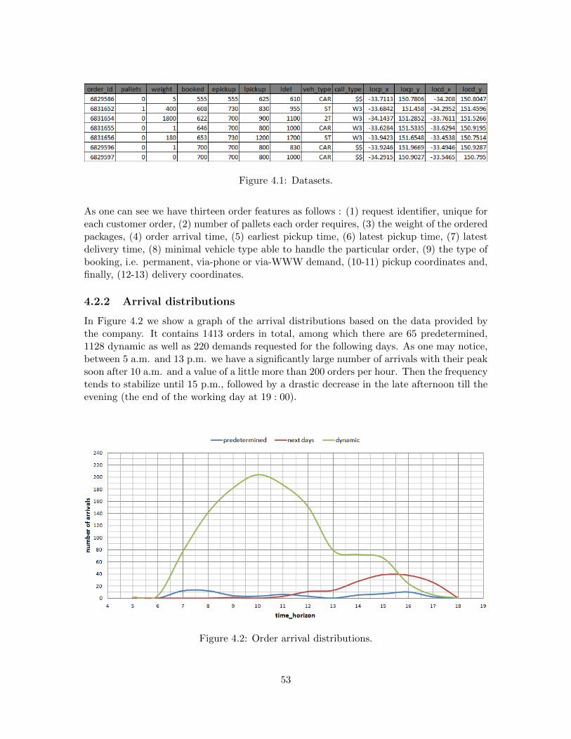
Figure 4.1: Datasets.

As one can see we have thirteen order features as follows : (1) request identifier, unique foreach customer order, (2) number of pallets each order requires, (3) the weight of the orderedpackages, (4) order arrival time, (5) earliest pickup time, (6) latest pickup time, (7) latestdelivery time, (8) minimal vehicle type able to handle the particular order, (9) the type ofbooking, i.e. permanent, via-phone or via-WWW demand, (10-11) pickup coordinates and,finally, (12-13) delivery coordinates.

4.2.2 Arrival distributions

In Figure 4.2 we show a graph of the arrival distributions based on the data provided bythe company. It contains 1413 orders in total, among which there are 65 predetermined,1128 dynamic as well as 220 demands requested for the following days. As one may notice,between 5 a.m. and 13 p.m. we have a significantly large number of arrivals with their peaksoon after 10 a.m. and a value of a little more than 200 orders per hour. Then the frequencytends to stabilize until 15 p.m., followed by a drastic decrease in the late afternoon till theevening (the end of the working day at 19 : 00).

Figure 4.2: Order arrival distributions.

53

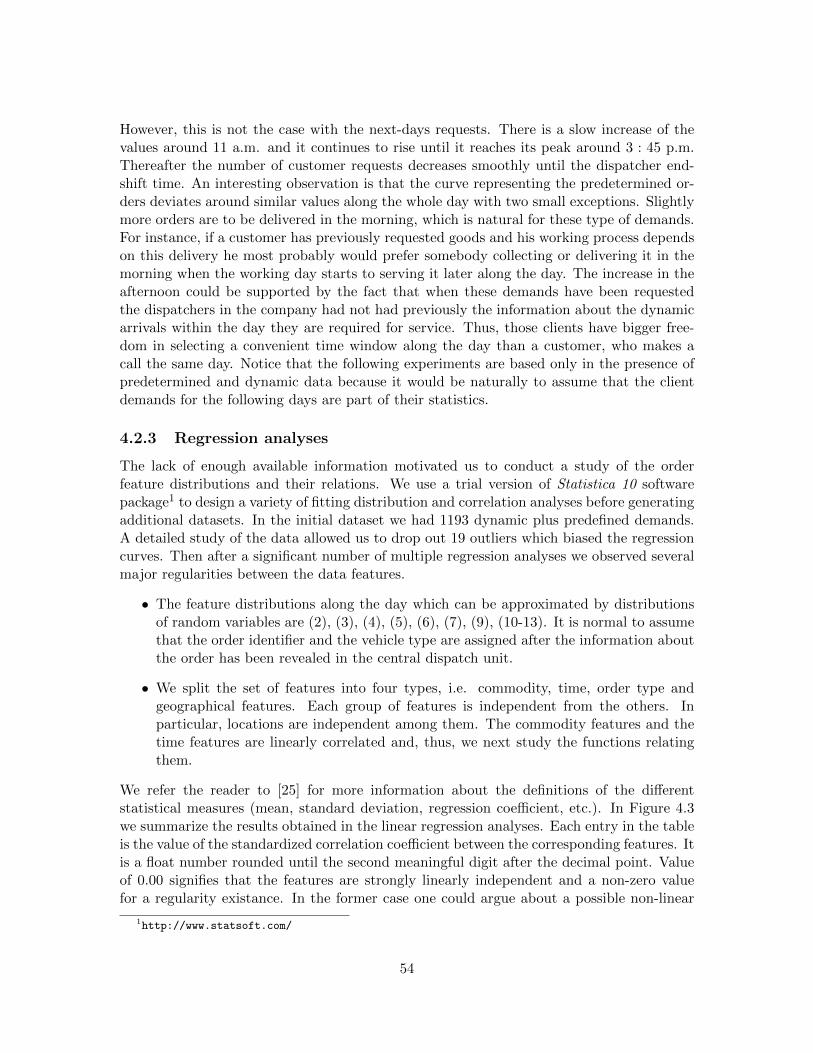
However, this is not the case with the next-days requests. There is a slow increase of thevalues around 11 a.m. and it continues to rise until it reaches its peak around 3 : 45 p.m.Thereafter the number of customer requests decreases smoothly until the dispatcher end-shift time. An interesting observation is that the curve representing the predetermined or-ders deviates around similar values along the whole day with two small exceptions. Slightlymore orders are to be delivered in the morning, which is natural for these type of demands.For instance, if a customer has previously requested goods and his working process dependson this delivery he most probably would prefer somebody collecting or delivering it in themorning when the working day starts to serving it later along the day. The increase in theafternoon could be supported by the fact that when these demands have been requestedthe dispatchers in the company had not had previously the information about the dynamicarrivals within the day they are required for service. Thus, those clients have bigger free-dom in selecting a convenient time window along the day than a customer, who makes acall the same day. Notice that the following experiments are based only in the presence ofpredetermined and dynamic data because it would be naturally to assume that the clientdemands for the following days are part of their statistics.

4.2.3 Regression analyses

The lack of enough available information motivated us to conduct a study of the orderfeature distributions and their relations. We use a trial version of Statistica 10 softwarepackage1 to design a variety of fitting distribution and correlation analyses before generatingadditional datasets. In the initial dataset we had 1193 dynamic plus predefined demands.A detailed study of the data allowed us to drop out 19 outliers which biased the regressioncurves. Then after a significant number of multiple regression analyses we observed severalmajor regularities between the data features.

• The feature distributions along the day which can be approximated by distributionsof random variables are (2), (3), (4), (5), (6), (7), (9), (10-13). It is normal to assumethat the order identifier and the vehicle type are assigned after the information aboutthe order has been revealed in the central dispatch unit.

• We split the set of features into four types, i.e. commodity, time, order type andgeographical features. Each group of features is independent from the others. Inparticular, locations are independent among them. The commodity features and thetime features are linearly correlated and, thus, we next study the functions relatingthem.

We refer the reader to [25] for more information about the definitions of the differentstatistical measures (mean, standard deviation, regression coefficient, etc.). In Figure 4.3we summarize the results obtained in the linear regression analyses. Each entry in the tableis the value of the standardized correlation coefficient between the corresponding features. Itis a float number rounded until the second meaningful digit after the decimal point. Valueof 0.00 signifies that the features are strongly linearly independent and a non-zero valuefor a regularity existance. In the former case one could argue about a possible non-linear

1http://www.statsoft.com/

54

connection between the respective features. However, this situation is refuted as well bythe conducted multivariate analyses. Next, the red-color decimal attributes show a strongcorrelation dependency amongst the time features. In particular, the earliest pickup, thelatest pickup and delivery times depend strongly on the arrival time. The latter result isnatural as these preferences are known only after a particular client states an order. Inaddition, it is likely that the latest times depend more on the earliest time than on thebooking time, which is confirmed by the higher values for these feature combinations. Wegive other piece of attention to the entries in green color, which stand for averagely positivelinear dependency between the order weight and the number of pallets it requires. Notethat the latter one is a discrete variable and, therefore, the value of the regression coefficientis hard to be interpreted as it is only defined for continuous stochastic samples. On theother hand this feature has enough distinctive values and, thus, we are pleased with theapproximation discovered. The reader is referred to [48] for more information about thedependency between two arbitrary random variables. Furthermore, we designed residualanalyses in order to improve the quality of the artificially generated datasets afterwards.

Figure 4.3: Regression matrix.

In order to uncover the process of generating the datasets in more details we next presenta general linear regression equation and discuss its components. By x and y we denote therespective predictor and dependant variables, by a and b the estimates of the real coefficientsobtained during the analyses and the last term, ε, represents the residual in these analyses.Usually, for large samples the error follows a normal distribution. Moreover, the coefficientshave a particular non-zero deviation, which approaching zero with higher values of theregression coefficient. We took all of these fine-grained observations when generating theorder tuples for our experiments.

y = a ∗ x+ b+ ε

4.2.4 Predictor distributions

In addition to the functional dependency results established above, we investigate in moredetail the distribution of the order arrival time and the order weight as being major sourcesimplying those regularities. The number of orders revealed during the day can be approx-imated by a non-homogenous and stationary Poisson process as in Figure 4.4 on the left.

55

On the horizontal axis the working hours are placed along the day, while on the vertical onethe cumulative number of arrivals for these periods. A nice consequence of this approxima-tion is that the order interarrival time follows an exponential distribution (see [49] for moredetails regarding this issue). However, this is not the case with the order weight feature,shown in Figure 4.4 on the right, which follows very steep Gamma distribution. Sligthlymore than 1000 orders are composed of less than a hundred kilograms each and all the restare distributed quite sparsely until a maximal value of 2000 kilograms. Recall, we removedsome of the observations, viz. so-called outliers, as they strongly biased the results obtainedregarding the regression between the weight and the pallets.

Figure 4.4: Arrivals and weight distributions.

4.2.5 Generated datasets

Here, we pinpoint some details about the creation of the additional datasets. Using thepreviously measured statistical results we created 330 datasets of orders, denoted as day1-day230 and pday100-pday200, which we describe next.

1. The files day101-day200 are used to test the performance of the dispatch rules beingimplemented. From now on we call every tuple within each of these datafiles a realorder.

2. The purpose of pday101-pday200 is to represent the stochastic model of the environ-ment for the datasets day101-day200. We refer to the individuals of this collectionof demands as seeming or ”fake” orders. In the process of creating these orders wealso take into account the descriptive statistics of the customer requests in day100-day200 as follows : pday101 is generated based on the statistics obtained for the daysday1-day100, pday102 on the distributional features for days day1-day101, and so on,

56

until the last dataset pday200, which is created using the descriptive numbers for daysday1-day199. In reality, the increase of the revealed information in the past days withrespect to the current date could help for a better prediction of the future demands.

3. The last thirty datasets, i.e. day201-230 will serve to assess the quality of the policieslearnt, as discussed in the experimental section of the next chapter.

Figure 4.5: Comparison of the original and the generated datasets.

In Figure 4.5 we compare the arrival distributions of the original information and a datasetobtained after we averaged the arrivals over the datafiles day101-day200. The histogram onthe left shows how much the two samples differ within each work hour, whereas the graphon the right gives a flavour about the similarity of their smooth distribution curves. Wealso report several descriptive statistics of the daily arrivals for all types of orders in Table4.1. The average number of real orders per dataset is 1192, which varies within the limits1074 and 1260. Between 12%-18% of them have been requested on previous days. Besidesthese numbers we have an average of 1183 ”fake” orders per day. We do not generate pre-requested seeming services because all of these are known at simulation time. The columnsmarked by a notation with index d are the statistics for the dynamic demands, whereasthose marked with p are the corresponding numbers for the known orders.

order type m σ min max mp σp minp maxp md σd mind maxd

real orders 1192 34 1074 1260 180 6 158 193 1012 29 907 1067

”fake” orders 1183 45 988 1274 1183 45 988 1274 0 0 0 0

Table 4.1: Real and seeming order statistics.

57

4.3 An Experimental Framework

A decision-support system in any area of the public or private sector should be carefullydesigned and must guarantee its efectiveness by giving qualified recommendations, whichrely on the overall current status. Usually such a system maintains a large number ofstatistics, which is a difficult task for the employees. On the other hand, the decisionsmade should be clear and easily understandable by the end-users. They also must not bemisleading or ambiguous as this would lead to mistakes when a final decision is to be made.The latter is of significant importance when a human life depends on such a supportedness.Although, this is not the case in our work, we are interested in verifying the quality of thedecisions made by the simple rules we implemented. In order to do so we first define a fewappropriate notions and notations, which we believe will help the reader to avoid a possibleconfusion later on. We also describe three pooling strategies under both scenarios, i.e. withand without the use of stochastic model.

4.3.1 Initial schedule

Let us denote all the orders executed in a particular day by O = {o1, . . . , on}. Part of thesedemands have been requested on some previous days, and therefore they are already knownin the morning when the dispatchers have started their shift. We denote these demands byI = {i1, . . . , ip}. At the beginning of the time horizon we produce a pickup and deliveryrouting and scheduling plan (PDRSP) PI for the set I. Also at the end of the working daywe create similar timetable for O, i.e. PO. The positions of the I-orders differ in PI andin PO. However, in the latter plan they are the desired ones as these are decided takinginto account all orders. Therefore, we are interested in a maximal matching between thepositions of the I-orders in both plans. However, in the morning of the working day wehave available only the set I, but not O. Nevertheless, we could predict how many orderswould arrive the same day using the past data statistics and in this way to improve thequality (with respect to the final plan) of the initial plan as follows : (1) generate a set ofadditional orders F , simulating the dynamic ones, (2) create a PDRSP PI∪F for F and I,and (3) project the set I in PI∪F .

4.3.2 Suboptimal schedule

During the heuristic evalution experiments we are concerned that each individual decisionabout a new order does not depend on possible wrong previous decisions. On the otherhand, at the end of the day we have at our disposal all the decisions for the past shift asif we knew them initially. Hence, for a particular dynamic time instant along the day wecould compare the dynamic heuristic decisions made regarding the new demands with thoseavailable at shift completion when an offline schedule is produced. The latter is done byusing the Indigo solver to create a schedule given a problem instance. It does so though acombination of heuristics which, given a problem specification, initially builds the vehicleassignments and then improves them using local search methodologies. At the end of thisprocess we have a visiting timetable for managing the fleet services. We call such a schedulesuboptimal plan.

58

4.3.3 Evaluation procedure

Let us think of a solution to a given ODPDP as a set of requests. We denote a suboptimalplan for the whole set O of n orders as S(O,n). We call the positions of the order requestsin this timetable suboptimal positions as they have been assigned under the assumption thatthe whole information is known in advance. Furthermore, let h ∈ H be an heuristic fromour repository. We would like to evaluate it in such a way that each individual decisionmade about a new customer is independent from the other past, current and future heuristicdecisions. A possibility to do that is the following : for ok ∈ O \ I we fix the orders in thesuboptimal plan S(O,n), which have arrived before the booking time tk of ok. We call thissubset of requests partial schedule or partial plan and we denote it by S(O,nk, tk), wherenk ≤ n is the number of orders arrived before tk. Then h makes a decision about where okcan be inserted and we compare that decision with the location of the same order in S(O,n).In this way, the decision made does not depend on possible wrong previous decisions as thepositions of the requests in S(O,nk, tk) are suboptimal. We must say that the decisionswe are dealing with are within the scope of vehicles. In other words, each decision simplyconcerns the vehicle that will serve the new loads. A more precise view would be to con-sider the precise positions along a vehicle route where the new requirements are positioned,but this approach would concentrate more on the local route features than the global ones,which are amongst our objectives. In this context, we consider that an heuristic decisionis correct if it corresponds to the vehicle that manages the particular order according toS(O,n). After making this comparison against the offline schedule S(O,n) we update thepartial plan S(O,nk, tk) by including the order ok in it.

In Figure 4.6 we depict the major procedure in our experimental setting. We start byfixing the known information, which is represented by the set I with p orders. The map-ping f : S × N → S represents this operation. It takes a solution S, a natural numbern0 (n0 ≤ n) and it returns a partial schedule for those n0 orders. Furthermore, withoutloss of generality we can assume that the dynamic orders O \ I = {o1, . . . , on−p} arrive insuccession (i.e. o1, o2 and so on until the last one on−p) and their arrival times are t1, t2,. . ., tn−p, respectively.

S(O,n)

S(O, p, t1) + o1

h1 . . . h8

0/1 . . . 0/1

S(O, p+ 1, t2) + o2

h1 . . . h8

0/1 . . . 0/1

. . . S(O,n− 1, tn−p) + on−p

h1 . . . h8

0/1 . . . 0/1

f f f

Figure 4.6: Evaluation procedure.

59

We have implemented eight dispatch rules and, hence, for each order ok ∈ O \ I every ruleshould make a decision. The latter is ranked as correct (1) or incorrect (0). Then the sameprocedure is activated for n0 + 1, n0 + 2, . . . , n−1 orders, respectively, until all the dynamicorders have been decided.

4.3.4 Request sequences

We now address request sequences and what we call a solution to a given ODPDP in termsof decisions. Recall, every working day in the company constitutes of finite knowledge aboutcustomer demands and, therefore, we are interested in finite request and decision sequences.

Definition 13 : (Request sequence) Let RO = {r1, . . . , r2∗n} be the set of requests for agiven set of orders O = {o1, . . . , on}. Then we call Rn = [r1, . . . , r2∗n] the request sequencecorresponding to RO. It cointains the requests from RO sorted by their arrival time.

Definition 14 : (Heuristic scheme) Let H be a repository of heuristics. Let alsoRn = [r1, r2, . . . , r2∗n] be a finite sequence of requests arriving in the system at the mo-ments t1, t2, . . ., t2∗n, respectively. Then a finite heuristic scheme to Rn is the decisionsequence dn = [d1, d2, . . . , dn], where dk ∈ H for k ∈ [1, n] is the decision made at timeinstant tk for managing the new order ok ∈ O.

Note that given a finite heuristic scheme there are | H | 2∗n instantiations of it. Thus wedefine the following notion of heuristic schedule.

Definition 15 : (Heuristic schedule) Let H be a repository of heuristics. Let also dn =[d1, d2, . . . , dn] is a finite heuristic scheme to the request sequence Rn = [r1, r2, . . . , r2∗n].Then a finite heuristic schedule to Rn is the heuristic sequence hn = [h1, h2, . . . , hn], wherehk for k ∈ [1, n] is a concrete heuristic from H (i.e. substitute dk for k ∈ [1, n] in dn by hk).

4.3.5 Solutions and partial solutions

The Indigo solver may produce a schedule when an input request sequence is given. Such aschedule not only assigns a finite heuristic solution to that sequence, but also contains ad-ditional information about the fleet timing at the client locations and details about vehiclerack-space availability. We capture this information with the following definitions.

Definition 16 : (Fleet schedule) Let Rn = [r1, . . . , r2∗n] be a request sequence and Hbe a repository of heuristics. Then we call the triple Sn = (hn,Rn, In) a fleet schedule(solution) to Rn, where hn is a finite heuristic schedule to Rn and the next two componentsconstitute a PDRSP Pn = (Rn, In) for Rn.

Recall, Rn contains the ordered vehicle request routes and In their itineraries. Each suchtimetable contains all the details about the fleet management for handling Rn and we callit schedule itinerary to Rn. Each unitary element rk in Rn is a request and ik in In is arequest itinerary. They are formalized as follows :

60

rk : < tk, qk, uk, [tke , tkl ], lk >

ik : < ak, wk, bk, sk, ek >,

where qk, uk, [tke , tkl ] and lk in the first tuple are, respectively, the pallets, the weight, the

time window and the location of rk. The second vector contains the features ak, wk, bk,sk, ek, which are the arrival, waiting, starting, service and leaving times at the location lk,respectively. Note that for each vehicle vj ∈ V , the route Rn

j = {rj1 , . . . , rjnj} ∈ Rn and its

itinerary Inj = {ij1 , . . . , ijnj} ∈ In are ordered sets. This observation allow us to unify them

with sequences of, respectively, requests [rj1 , . . . , rjnj] and unitary itineraries [ij1 , . . . , ijnj

].

Thus, the solution to a request sequence is a pair of heuristic schedule together with apickup and delivery routing and scheduling plan for managing this sequence. The mainidea behind the above definition is that each request sequence represents a routing problemand a solution to this instance contains two components. The first component represents avehicle allocation of the orders in the particular plan, whereas the second one expresses thefleet execution plan itself.

Recall that V = {v1, . . . , vm} is the set of vehicles and that each member vj of this set canbe assigned to exactly one visiting sequence. Also, recall, that any two vehicles vj1 , vj2 ∈ Vcannot have common assignments, i.e. they cannot process the same requests at any timepoint. Hence, one may be interested in the solution for a specific vehicle or even a vehicletype, which is expressed by the following definition.

Definition 17 : (Vehicle schedule) Let vj ∈ V be a vehicle, which according to thesolution Sn = (hn, Pn) to Rn processes the request sequence Rn

j = [rj1 , rj2 , . . . , rjr ] withj1 < j2 < . . . < jr. Then we call the heuristic schedule hnj = [h∗1, . . . , h

∗n] a projection of hn

onto the route of vj . Each element h∗k is defined as follows : (1) it is hk if k ∈ {j1, . . . , jr}and (2) ε (no decision is made about rk) otherwise. Then a schedule of vehicle vj is thetriple Sn

j = (hnj , Rnj , I

nj ).

As we mentioned at the beginning of Section 4.3.3, given a solution to a routing problemwe are interested in the projection of that schedule over some of the orders. Thus we nextdefine the notion of partial schedule or partial solution to a given request sequence.

Definition 18 : (Partial fleet schedule) Let Sn = (hn,Rn, In) be a solution to Rn =[r1, . . . , r2∗n]. Then the triple Sn,p = (hn,p,Rn,p, In,p) is called partial fleet schedule ora partial solution to Rn over the first p ∈ [1, n] orders. It is defined as follows : (1)hn,p = [h1, . . . , hp, ε, . . . , ε], where for each k ∈ [1, p] we have that hk ∈ hn and (2) Rn,p andIn,p are, respectively, the projections of Rn and In over the first p requests.

Note that Sn,p = (hn,p, Pn,p) is also a solution to the input sequence Rp = [r1, . . . , rp]. How-ever, it it not suboptimal solution to that request sequence. Rather than, it just containsinformation about the requests arrived by the time tp+1 when op+1 has occured. In theterms we used in Section 4.3.3 each position of a request in Sn,p is called suboptimal andSn,p = S(O, p, tp+1).

61

In order to avoid further confusions when we work with both types of solutions we willrefer to the firstly defined notion as a complete solution to a given request sequence. If nosuch ambiguity exists, we will keep refering it as just a solution to that sequence. In whatfollows, we define the notion of heuristic correctness, which serves as an evaluation measureof the dispatch rules from our repository.

4.3.6 Heuristic correctness

Here, we suggest several measures to evaluate the ”distance” of a local heuristic decisionwith respect to an offline local and global suboptimal solutions. Generally, we have an orderok ∈ O arrived in the moment tk, a suboptimal plan S(O,n) and a projection S(O,nk, tk)of it over the nk orders known before tk. Moreover, let H be the repository of the dispatchrules and HIndigo = {hIndigo} be the heuristic, whose result is obtained by the combinedefforts of the solver to assign a new order.

Definition 19 : (Precise vehicle measure) Let V = {v1, . . . , vm} be the consideredfleet. Then we call a precise valuation function the mapping f1 : V × V → {0, 1}, definedas follows :

• f1(vj , vk) = 1, if j = k

• f1(vj , vk) = 0, otherwise.

This measures assigns 1 only if the two arguments coincide and 0, otherwise. Although,the value can be zero, it might be the case that exists a suboptimal plan, which is some-how symmetric to the produced one (i.e. S(O,n)) and where the new demand is actuallyassigned a vehicle of the same type. Thus, we proceed by defining a vehicle type measurein order to break this kind of symmetry with respect to the type characteristic of the fleet.Note that in the latter case we capture a large set of suboptimal solutions.

Definition 20 : (Vehicle type measure) Let V = {v1, . . . , vm} be the considered fleet.Then we call a type valuation function the mapping f2 : V × V → {0, 1}, defined as follows:

• f2(vj , vk) = 1, if vj and vk are of the same type

• f2(vj , vk) = 0, otherwise.

The two measures above capture a large number of more or less identical suboptimal so-lutions. Apart from them one could also argue that exist a suboptimal solution where thenew order is handled by a vehicle, which has different, but still feasible type. The latterobservation could contribute to determine whether a particular rule has made a good deci-sion or not. Since in our fleet there is a large number of vehicles able to accommodate anynew demand we only consider those passing close to both the target and the destinationlocations of the new order. Therefore, we define a third measure to capture this kind ofsolution similarity.

62

Definition 21 : (Geographical type measure) Let V = {v1, . . . , vm} be the consideredfleet and oi ∈ O be an order. Then we call a geographical valuation function the mappingf3 : V × V → {0, 1}, defined as follows :

• f3(vj , vk) = 1, if vj and a vehicle, geographically close to vk with respect to oi are ofthe same type

• f3(vj , vk) = 0, otherwise.

All the measures f1, f2 and f3 give valuations of the dispatch rules from H with respectto a suboptimal plan produced at later moment within the working day. Next, using thenotion of valuation function we define the correctness of an heuristic decision.

Definitions 22 : (Heuristic correctness) Let h ∈ H be a dispatch rule, V = {v1, . . . , vm}be the fleet and f : V × V → {0, 1} be a valuation function. Also let in moment tk a neworder ok ∈ O arrives and S(O,nk, tk) be the partial plan for the orders known before tk.Then, if vk = h(S(O,nk, tk), ok), vIndigo = hIndigo(S(O,n), ok) and f(vk, v

Indigo) = 1, wecall that h is correct with respect to S(O,n), ok and the Indigo solver. Otherwise, we callthat decision incorrect.

4.4 Experimental Results

In this section we consider three pooling strategies, i.e. once-a-day, time-zones, fixed-time-span. For each of them we consider two scenarios, i.e. with and without simulating seemingneeds. We evaluate the heuristics performance within each scenario for every strategy. Re-call that time-zones and fixed-time-span strategies are represented by multiple time slices.The procedure depicted in Figure 4.6 assumes the availability of one suboptimal plan.However, one can argue that comparing against this plan is insufficient for a meaningfulheuristic ranking. Thus, at each time slice boundary in every setting we produced 5 subop-timal plans, against which we evaluate the correctness of each rule. The latter give us theability to rate the dispatch rules regarding the different valuation measures (precise, vehicletype and geographical) not only by assigning a boolean value to each of them, but a numberranging between 0 and 5. In addition, we report a set of descriptive statistics regarding theaverage individual heuristic cost per order, average heuristic cost per time slice, etc.. Allthese numbers allow us to decide which pooling strategy, among the presented, probablywill give the best performance in practice.

We present some notation we are going to use in order to give a more formal view in thefollowing sections. Let O be the set of n orders and T be the working time horizon. Thenfor a time slice boundary (time instant along the day) ti ∈ T we denote by On

≤i the set oforders arrived before ti, by On

i the set of orders arrived within the i-th time slice and byOn

>i the set of orders after ti. As in the different cases we need to distinguish the real andthe unreal (”fake”) demands we adopt the following notation for them : (1) by R we denotethe set of nR real demands and (2) by D the set of nD seeming orders.

63

4.4.1 Once-a-day strategy

This scenario presents a scheme in which we reoptimize once during the working day, viz.at the end of the shift. That is, T = [t0, t1] = [5:00, 19:00] or the entire dispacher shift,between 5:00 and 19:00, is one time slice. In addition, the only information available before5:00 are the predetermined customer demands I = {i1, . . . , ip} and we assume that the newdemands after 19:00 are collected for the subsequent days. Note that this does not meanthat no orders are served after this time. It might be the case that a vehicle has collected apackage and the delivery will be realized in an after-shift time. Also note that this poolingstrategy is not likely to be executed in practice due to the high dynamicity of the problemwe deal with and the large number of the arriving client demands. It is possible that duringthe day the accumulated number of wrong heuristic decisions is sufficiently large and leadto a bigger and bigger deviation from the desired final values. Although, this fact, we areinterested in calculating an heuristic performance baseline, to which we can compare therest of the pooling scenarios and, thus, once-a-day is the perfect candidate to do that.

Without Probabilistic Model In this case we consider only the presence of real cus-tomer demands. Then the setting can be expressed as follows :

(S(R, p, t0), R \ I, ∅), (S(R,nR), ∅, ∅),

where p is the number of real orders before t0 (i.e. 5:00). Note that the number of triplecorrespond to the number of time slice boundaries. The first component is a suboptimalor partial plan, the second one is the set of orders arrived within the considered time sliceand the third one is aimed to represent the seeming orders when incorporated. Thus, thedispatch rules are evaluated only within one interval (i.e. [t0, t1]).

With Probabilistic Model Here we consider the case when some seeming orders aresimulated and, hence, the scheme is the following :

(S(R ∪D, p+ nD, t0), R \ I,D), (S(R ∪D,nR + nD), ∅, ∅)

This time the number in R ∪D we fix the initial p real demands and all the unreal ones.As opposed to the previous case the third component of the first triple is non-empty. Thatis, it contains the set of all the seeming requirements arrived after t0. Also one can noticethat the first components differ. The reason for that is due to the fact that a suboptimalschedule is produced for both the real and unreal requirements, whereas in the previoussetting we consider only the set of real orders.

4.4.2 Time-zones strategy

As we mentioned above once-a-day scenario could serve as a good baseline to which onecan compare other realizations of the time slices ideology. Another benefit of it couldbe in case we deal with a problem which is characterized by a lower dynamicity of thearriving customer requests than ours. In this case the wrong dispatch decisions would beless and it is more likely to achieve a particular objective. Nevertheless, this is not thecase with the problem we deal with and, thus, we consider daily time zones, which split the

64

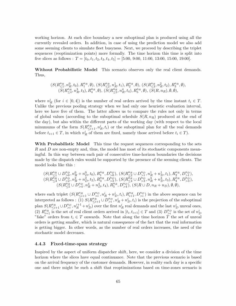
working horizon. At each slice boundary a new suboptimal plan is produced using all thecurrently revealed orders. In addition, in case of using the prediction model we also addsome seeming clients to simulate fleet busyness. Next, we proceed by describing the tripletsequences (reoptimization points) more formally. The time horizon this time is split intofive slices as follows : T = [t0, t1, t2, t3, t4, t5] = [5:00, 9:00, 11:00, 13:00, 15:00, 19:00].

Without Probabilistic Model This scenario observes only the real client demands.Thus,

(S(RnR≤1 , n

0R, t0), RnR

1 , ∅), (S(RnR≤2 , n

1R, t1), RnR

2 , ∅), (S(RnR≤3 , n

2R, t2), RnR

3 , ∅),(S(RnR

≤4 , n3R, t3), RnR

4 , ∅), (S(RnR≤5 , n

4R, t4), RnR

5 , ∅), (S(R,nR), ∅, ∅),

where niR (for i ∈ [0, 4]) is the number of real orders arrived by the time instant ti ∈ T .Unlike the previous pooling strategy when we had only one heuristic evaluation interval,here we have five of them. The latter allows us to compare the rules not only in termsof global values (according to the suboptimal schedule S(R,nR) produced at the end ofthe day), but also within the different parts of the working day (with respect to the localminumums of the form S(RnR

≤i+1, niR, ti) or the suboptimal plan for all the real demands

before ti+1 ∈ T , in which niR of them are fixed, namely those arrived before ti ∈ T ).

With Probabilistic Model This time the request sequences corresponding to the setsR and D are non-empty and, thus, the model has most of its stochastic components mean-ingful. In this way between each pair of consecutive time-horizon boundaries the decisionsmade by the dispatch rules would be supported by the presence of the seeming clients. Themodel looks like this :

(S(RnR≤1 ∪D

nD>0 , n

0R + n0

D, t0), RnR1 , DnD

>0 ), (S(RnR≤2 ∪D

nD>1 , n

1R + n1

D, t1), RnR2 , DnD

>1 ),

(S(RnR≤3 ∪D

nD>2 , n

2R + n2

D, t2), RnR3 , DnD

>2 ), (S(RnR≤4 ∪D

nD>3 , n

3R + n3

D, t3), RnR4 , DnD

>3 ),

(S(RnR≤5 ∪D

nD>4 , n

4R + n4

D, t4), RnR5 , DnD

>4 ), (S(R ∪D,nR + nD), ∅, ∅),

where each triplet (S(RnR≤i+1 ∪D

nD>i , n

iR + niD, ti), R

nRi+1, D

nD>i ) in the above sequence can be

interpreted as follows : (1) S(RnR≤i+1 ∪D

nD>i , n

iR +niD, ti) is the projection of the suboptimal

plan S(RnR≤i+1∪D

nD>i , n

i+1R +niD) over the first niR real demands and the last niD unreal ones,

(2) RnRi+1 is the set of real client orders arrived in [ti, ti+1] ∈ T and (3) DnD

>i is the set of niD”fake” orders from ti ∈ T onwards. Note that along the time horizon T the set of unrealorders is getting smaller, which is natural consequence of the fact that the real informationis getting bigger. In other words, as the number of real orders increases, the need of thestochastic model decreases.

4.4.3 Fixed-time-span strategy

Inspired by the aspect of uniform dispatcher shift, here, we consider a division of the timehorizon where the slices have equal continuance. Note that the previous scenario is basedon the arrival frequency of the customer demands. However, in reality each day is a specificone and there might be such a shift that reoptimizations based on time-zones scenario is

65

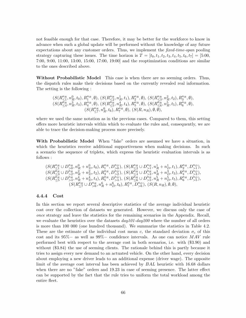
not feasible enough for that case. Therefore, it may be better for the workforce to know inadvance when such a global update will be performed without the knowledge of any futureexpectations about any customer orders. Thus, we implement the fixed-time-span poolingstrategy capturing these issues. The time horizon is T = [t0, t1, t2, t3, t4, t5, t6, t7] = [5:00,7:00, 9:00, 11:00, 13:00, 15:00, 17:00, 19:00] and the reoptimization conditions are similarto the ones described above.

Without Probabilistic Model This case is when there are no seeming orders. Thus,the dispatch rules make their decisions based on the currently revealed real information.The setting is the following :

(S(RnR≤1 , n

0R, t0), RnR

1 , ∅), (S(RnR≤2 , n

1R, t1), RnR

2 , ∅), (S(RnR≤3 , n

2R, t2), RnR

3 , ∅),(S(RnR

≤4 , n3R, t3), RnR

4 , ∅), (S(RnR≤5 , n

4R, t4), RnR

5 , ∅), (S(RnR≤6 , n

5R, t5), RnR

6 , ∅),(S(RnR

≤7 , n6R, t6), RnR

7 , ∅), (S(R,nR), ∅, ∅),

where we used the same notation as in the previous cases. Compared to them, this settingoffers more heuristic intervals within which to evaluate the rules and, consequently, we areable to trace the decision-making process more precisely.

With Probabilistic Model When ”fake” orders are assumed we have a situation, inwhich the heuristics receive additional supportiveness when making decisions. In sucha scenario the sequence of triplets, which express the heuristic evaluation intervals is asfollows :

(S(RnR≤1 ∪D

nR>0 , n

0R + n0

D, t0), RnR1 , DnD

>0 ), (S(RnR≤2 ∪D

nR>1 , n

1R + n1

D, t1), RnR2 , DnD

>1 ),

(S(RnR≤3 ∪D

nR>2 , n

2R + n2

D, t2), RnR3 , DnD

>2 ), (S(RnR≤4 ∪D

nR>3 , n

3R + n3

D, t3), RnR4 , DnD

>3 ),

(S(RnR≤5 ∪D

nR>4 , n

4R + n4

D, t4), RnR5 , DnD

>4 ), (S(RnR≤6 ∪D

nR>5 , n

5R + n5

D, t5), RnR6 , DnD

>5 ),

(S(RnR≤7 ∪D

nR>6 , n

6R + n6

D, t6), RnR7 , DnD

>6 ), (S(R,nR), ∅, ∅),

4.4.4 Cost

In this section we report several descriptive statistics of the average individual heuristiccost over the collection of datasets we generated. However, we discuss only the case ofonce strategy and leave the statistics for the remaining scenarios in the Appendix. Recall,we evaluate the heuristics over the datasets day101-day200 where the number of all ordersis more than 100 000 (one hundred thousand). We summarize the statistics in Table 4.2.These are the estimate of the individual cost mean c, the standard deviation σc of thiscost and its 95%− as well as 99%− confidence intervals. As one can notice MAV ruleperformed best with respect to the average cost in both scenarios, i.e. with ($3.90) andwithout ($3.84) the use of seeming clients. The rationale behind this is partly because ittries to assign every new demand to an actuated vehicle. On the other hand, every decisionabout employing a new driver leads to an additional expense (driver wage). The oppositelimit of the average cost interval has been achieved by BAL heuristic with 16.68 dollarswhen there are no ”fake” orders and 19.23 in case of seeming presence. The latter effectcan be supported by the fact that the rule tries to uniform the total workload among theentire fleet.

66

Without Model With Model

5-19:00 5-19:00

h c [$] σc 95%− 99%− c [$] σc 95%− 99%−MIN 3.99 4.43 [3.96,4.02] [3.95,4.03] 4.30 5.93 [4.26,4.34] [4.25,4.35]

BAL 16.68 7.23 [16.66,16.71] [16.65,16.72] 19.23 11.29 [19.19,19.26] [19.18,19.28]

SHIFT 9.45 4.65 [9.43,9.48] [9.42,9.49] 9.89 6.13 [9.86,9.93] [9.85,9.94]

CUR 7.07 4.22 [7.04,7.10] [7.03,7.11] 8.10 4.34 [8.06,8.14] [8.05,8.15]

GEO 13.04 8.76 [13.02,13.07] [13.01,13.08] 13.91 9.36 [13.87,13.94] [13.86,13.95]

IMM 9.42 4.95 [9.40,9.45] [9.39,9.46] 10.41 6.02 [10.37,10.44] [10.36,10.45]

MAV 3.84 3.84 [3.81,3.87] [3.80,3.88] 3.90 3.90 [3.86,3.93] [3.85,3.95]

RAND 10.38 5.69 [10.35,10.41] [10.34,10.42] 11.38 7.33 [11.35,11.42] [11.33,11.43]

Table 4.2: Once-a-day pooling strategy : cost statistics.

Thus, it is quite likely a new vehicle to be actuated, which leads to undesired costs for thedriver’s wage. Due to the large number of individuals in our experiments the length of theconfidence intervals vary only between 5 and 10 AUS cents. Therefore, we can be quiteconfident about the average individual heuristic cost. Even we can make an estimate ofthe overall final cost using the means in Table 4.2 as follows : (1) calculate the individualcost averaged over the heuristics, i.e. 9.23 and 10.14 for the cases of without and with theseeming model, respectively, and (2) if we expect 1000 orders within a given day, then theexpected cost for serving them should vary between 9230 and 10140 dollars. Note thatthe last are just benchmarks assuming that each rule has been applied an equal numberof times during the day. Another interesting observation is about the cost increase in caseof having simulated demands. The reason for that is due to the higher number of orders.For instance, a vehicle elapses the distance between two real demands, according to thesuboptimal plan for reals, cheaper than according to the suboptimal plan for the real andthe unreal requirements. The idea is that between two consecutive real errands in the latterplan there can be multiple ”fake” orders and, thus, the travel costs are higher.

4.4.5 Time performance

In what follows we briefly discuss the time performance of the implemented dispatch rules.In Table 4.3 we report the numbers (in miliseconds) obtained within the once-setting. Theyare averaged over all the evaluation data. In the case when we do not benefit from thestochastic model, the rules perform significantly faster. The reason is partly because wehave shorter vehicle routes as well as smaller number of active vehicles than in a case withunreal demands. However, in both cases the CUR rule needed quite a lot of time, whichis expected since every time an order arrives at the system this heuristic decides not onlywhere to assign it, but also how to rearrange the remaining demands. Among the rest ofthe rules we have that IMM is at the first place when there are no ”fake” orders, which canbe explained due to the attempts it makes to assign every new order as soon as possible.

67

However, in the situation with seeming errands IMM is outperformed by SHIFT heuristic,possibly due to the decreased overall waiting time at customer locations. In the latter casethere are less possibilities for the new demand to be inserted and, thus, the CPU timeneeded by SHIFT rule decreases. On the other ”edge” of the time scale (except CURrule) stands MIN dispatch heuristic with maximum values of 33.29 miliseconds in the firstline and 116.44 miliseconds in the second one.

model MIN BAL SHIFT CUR GEO IMM MAV RAND

no 33.29 27.69 10.73 ≥2∗104 12.52 9.15 27.97 18.27

yes 116.44 100.85 15.33 ≥3∗104 27.8 15.57 91.93 54.31

Table 4.3: Once-a-day pooling strategy : time performance.

As one can notice the rules give recommendations in a reasonable time with respect to thetime the particular demand is requested (the time the calling lasts). We believe that onecan conclude similar results in time-zones- and fixed-time-span-settings and, therefore, wedo not present these.

4.4.6 Correctness

The notion of heuristic correctness is schedule-dependent. That is, a given dispatch rulewill perform differently with respect to distinct suboptimal plans. Thus, for each time sliceboundary in each scenario (i.e. with and without the seeming model) and a pooling strategy(once, time-zones, fixed-time-span) we produced 5 suboptimal plans. Besides this issue foreach valuation function (precise f1, vehicle f2 and geographical f3 types) we investigatetwo kinds of comparisons. The first one is with respect to the local incomplete oracles,positioned at the time slice boundaries. They know the 5 plans at the respective time or,equivalently, some partial information about the real demands. The other type of measureis with respect to the complete oracle, who knows all information in advance, i.e. the 5suboptimal plans at the end of the day. The latter kind is more important as in practice itwould give us a real view on how many correct decisions have been made during the lastday. However, the former is also important because it would allow us to pursue local desiresbesides global ones. One may be interested in a learning process, whose goal is to achievesome desired total costs by following a policy which selects an action taking into accountboth global and local measures.

Global correctness

This section puts forward a comparison of the global results obtained during the experi-ments. In Tables 4.4, 4.5 and 4.6 we report the average values of (1) the precise hits for eachheuristic (the value of f1) and (2) the vehicle type plus the geographical type evaluationresults (f2 + f3) for both scenarios. i.e. with and without expected client needs (pday101-pday200). We accumulate the values of f2 and f3 since both of them concern compatiblevehicle types, however, we lose some more detailed information about the correct hits.

68

Without Model With Model

5-19:00 5-19:00

h f1 f2 + f3 f1 f2 + f3

MIN 293 674 265 703

BAL 6 403 2 450

SHIFT 38 577 39 654

CUR 581 874 575 910

GEO 88 625 77 650

IMM 75 616 43 661

MAV 303 666 281 698

RAND 101 571 86 615

Table 4.4: Once-a-day pooling strategy : global valuation statistics.

Without Model With Model

5-19:00 5-19:00

h f1 f2 + f3 f1 f2 + f3

MIN 347 591 273 628

BAL 5 388 2 399

SHIFT 48 551 45 593

CUR 615 731 597 652

GEO 89 554 80 582

IMM 78 581 46 616

MAV 360 581 291 614

RAND 113 525 89 554

Table 4.5: Time-zones pooling strategy : global valuation statistics.

Without Model With Model

5-19:00 5-19:00

h f1 f2 + f3 f1 f2 + f3

MIN 348 563 281 620

BAL 5 366 2 388

SHIFT 49 521 46 581

CUR 632 649 550 689

GEO 89 528 83 576

IMM 79 557 47 607

MAV 361 554 299 607

RAND 113 499 93 545

Table 4.6: Fixed-time-span pooling strategy : global valuation statistics.

69

The first observation we would like to discuss is regarding the decrease in the precise num-bers when the stochastic model is used. Note that the presence of seeming errands addsan additional workload to the overall fleet. Thus, when Indigo produces a suboptimal planfor this higher number of demands it may significantly disalocates the vehicles with respectto a situation, in which vehicles carry only real packages. Consequently, in the former casethe precise vehicle route is more likely to be mistakenly guessed by a heuristic. However,the benefit of the model is observed if one compares the type valuation measures (i.e. thecolumns 2 and 4 in the tables). When the predictor is in force the correct decisions re-garding the vehicle type are more. Hence, the model is useful to predict the least vehicletype to which a new order need to be assigned. This is advantageous as it restricts thefleet of vehicles to a proper subset. Another positive observation is that reoptimizing morethan once per day leads to an increase of the precise valuation indicators. Note that thesenumbers in time-zones pooling strategy are noticeably higher than in once scenario and arequite similar to fixed-time-span statistics. Hence, introducing few time slices is beneficial,while many of them do not improve much the statistics. As opposed to this, the vehicletype measures tend to decrease when multiple reoptimizations are performed.

We continue with an heuristic comparison within the different pooling strategies. The CURrule performed best regarding all the measures (f1, f2 and f3) in all strategies. The latter isexpected as Indigo applies a combination of heuristic approaches when placing the requests,while we are using simple heuristics to achieve that result. However, on the second and thirdplaces regarding the precise measure are MAV and MIN, respectively. MAV scores between303 and 361 correct hits when the model is not used, and between 281 and 299 otherwise.The numbers for MIN are similar with range of [293, 348] when seeming clients are absent,and [265, 281] otherwise. According to the vehicle type measure the results are not so dis-tinguishable. In all cases we have high numbers, however, some of them must be noticed.For instance, CUR achieves 874 correct hits in once-setting with the stochastic model and910 without using it. These values decrease when multiple time slices are used. At thesecond position in this setting is MIN with 674 and 703 regarding the different scenarios,followed by MAV with 666 and 698. In the other two settings most of the results are gettingfuzzy (with respect to f2 + f3).

BAL rule performed worst in all settings. The rationale behind this is partly because therule tries to distribute the current total workload and, thus, the probability of actuating anew vehicle is high. However, this is not among the invariants Indigo uses when it evaluatesthe overall current status and inserts a new errand. An interesting observation is that wecan view the hits each rule achieves as a measure of covering between our heuristics and themethods implemented in the oracle. From this perspective, it is possible that BAL heuristicperforms better with respect to another VRP solver.

4.4.7 Global vs. local correctness

At the beginning of Section 4.4.6 we mentioned a possibility of an heuristic evaluation withrespect to the local minimums. These are computed by incomplete oracles (regarding theentire information), positioned at the time slice boundaries (at moments when a reoptimiza-

70

tion is performed).In this section we compare the global with these local heuristic correctdecisions made in the different scenarios. Although, this comparison is only with respect tothe overall daily statistics, we refer the inquisitive reader to the Appendix where we reportmany more numbers regarding the different time slices. The last could be used to comparethe dispatch rules within a particular time slice rather than only a comparison based on theentire-day statistics.

Without Model With Model

5-19:00 5-19:00

h local global local global

MIN 661 591 709 628

BAL 296 388 380 399

SHIFT 436 551 582 593

CUR 658 731 723 652

GEO 850 554 868 582

IMM 487 581 598 616

MAV 660 581 704 614

RAND 545 525 627 554

Table 4.7: Time-zones pooling strategy : global vs. local statistics.

Without Model With Model

5-19:00 5-19:00

h local global local global

MIN 659 563 724 620

BAL 292 366 389 388

SHIFT 433 521 593 581

CUR 673 649 782 689

GEO 847 528 885 576

IMM 483 557 609 607

MAV 659 554 720 607

RAND 543 499 640 545

Table 4.8: Fixed-time-span pooling strategy : global vs. local statistics.

Note that we report the statistics only for the multiple-slice scenarios because when wereoptimize only once during the day the local minimum coincide with the global one and,thus, the values of the local and the global valuations coincide. In Tables 4.7 and 4.8 we givethe local and the global values for the accumulated vehicle type valuation function (f2 +f3)in both the time-zones- and fixed-time-span-strategies. As one can notice the numbers arequite fuzzy. Some of the rules perform better (MIN, GEO, MAV, RAND in both timehorizon divisions and in addition CUR in fixed-time-span setting) and other worse (BAL,SHIFT, IMM in time-zones and fixed-time-span, and CUR only in time-zones) with respect

71

to the global values. We believe this random behaviour is due to the constraints each ruleimposes when evaluates the current schedule and, thus, some of them benefit from the localand other from the global ”knowledge” about the demands. In addition, we underline thatGEO performed significantly better (more than 847 correct hits) with respect to the localminimums than the global ones. We believe this is because it considers features similar tothe ones Indigo does.

4.5 Summary

In conclusion we summarize our efforts in this chapter. We study the feature distributionsin the original dataset provided by the company and based on the statistics obtained wegenerated 330 datasets which suit our problem instance. Then we discuss some issues relatedto the quality of the Indigo solutions followed by the heuristic evaluation procedure we usedin all the three pooling strategies (once, time-zones and fixed-time-span). We proceed bydefining several notions extending our theoretical framework in Section 2.1. Among theseare solution and partial solution, which we use to formalize the different strategies. Werank the implemented heuristics according to three valuation measures, i.e. precise, vehicletype and geographical. Using these we define the notion of heuristic correctness used inthe evaluation settings thereafter. Each heuristic decision is compared with respect to tensuboptimal plans (5 with and 5 without ”fake” orders) produced at each time slice boundary.We report some major statistics in the main body of the thesis and present the rest in theAppendix. Among these are (1) the average individual cost each heuristic achieves whenassigning a new order, (2) the time performance of the rules and (3) their global and localcorrectness results. We conclude by presenting a comparison between the local and theglobal rule performances in terms of correct decisions.

72

Chapter 5

Learning Experiments

Learning is the engine of life.by Martin Aleksandrov

This chapter gives a flavor on how we can learn dispatch policies within the framework wework with. We start with a short introduction on machine learning approaches and addressrecently emerging adaptive dynamic programming, which overcomes some of the drawbacksin the classical setting.

The main goal of our work is to learn how heuristic decisions depend on fleet and currentschedule features, to be able, given the parameters of the vehicles and their routes, to decidewhich rule will perform best. Given the distribution of decisions based on the past data,there is no expert able to say which rule has better local influence on the final route realiza-tions at the end of the day, hence we learn exactly that distribution of heuristic decisions.As a learning instrument we used Artificial Neural Networks (ANNs) to approximate thedecision distribution density function for each time-horizon division setting, i.e. once-a-day,time-zones and fixed-time-span. Regarding selected features, we consider some that appearmore informative, such as the number of active vehicles, free capacity of the nearby vehicles,etc. We trained our ANNs on a hundred days of past data and, thereafter, we tested themon a disjoint collection of thirty distinct days.

We continue with the description of the recommendation system we designed and the dif-ferent dispatch policies implemented : MaxSumPG, MaxSumPLG, MinSumPG andMinSumPLG. Each one of them implements solutions, which we compare with theirsuboptimal variants produced by Indigo. As a measure of comparison we present variousstatistics such as the value of information, overall waiting time, etc.. Finally, we concludethis chapter with a summary of the results obtained.

5.1 Machine Learning

In the last decades, more and more practitioners are trying to automate the process ofcomputer comprehension and interpretation of texts, pictures, voice, etc. The reason for

73

that is partly because of the tremendously increasing amount of information, which needsto be reasoned about and, in addition, the unability for a human being to process such hugeinformation to achieve some desired and specific objectives. A machine learning programcan be defined as a computer program, which improves its performance at some task throughsome experience ([46]). Learning programs are used when humans are unable to code theirexpertise in a deterministic algorithm (e.g., speech recognition, medical diagnosis, etc.)or the solution to the problem instance changes in time (spam filters, forecast of energyconsumption, etc.), or even when human expertise does not exist (e.g., exploring scientificdomains, navigating a robot on Mars, etc.). Thus, the experience can be evaluated by anexpert in the domain or it can be represented as an open-interpretative. The former typeof learning is called supervised, while the latter unsupervised. Many efforts are made instudying the properties of the different learning mechanisms. Although, this is not amongstour goals, we underline that for having a good model one definitely needs enough data,representing the experience of the machine learning program. The more experienced theprogram is, the better results it produces when an unobserved individual is input to it. Inother words, the quality of the query answer strongly depends on the information.

5.2 Neural Network

Artificial Neural Network is a mathematical model intensively used in the field of ArtificialIntelligence. Its main goal is to simulate the neural dendrites in the human brain, albeit amain difference is that while the model has a particular structure and the ”cells” exchangeinformation synchronously, the neurons in the brain network are chaotically distributed andinteract asynchronously. Although, there are many specific applications of Neural Networks,the main goal behind the model is learning a particular unknown-in-advance and arbitraryfunction by presenting multiple examples of it to the net. For example, Holldobler et al.in 1999 ([30]) applied a 3-layered recurrent neural network in order to approximate thesemantics of a given propositional logic program. The latter can be characterized as afixed-point of a continuous function (immediate consequence operator) operating over theundelying program lattice. Another instance can be found in [53], where Riedmiller S. andRiedmiller M. investigate neural reinforcement approach to learn local dispatching policiesin production scheduling. They relate the process of achieving local objectives with thesatisfaction of global properties, which resulted in better scheduling specifications. Neuralnetworks are also applied in the area of network communications. In particular, when thedesired objective is maintaining the flow of information in the so-called network backbone(Wilde, 1998, [57]) or learning hybrid-protocols in wireless/cordless environments (Kojic etal., 2012, [39]). Although, there are many applications in networking, artificial intelligenceand production scheduling areas, we are not aware of significant neural research in logistics.The latter motivated us to use that particular model in order to learn the function, whichselects the right action to be executed whenever a new event happens, i.e. new orderoccurs. We do not present any detailed discussion on the architecture of the network weused. Instead, we view it as a black box, which ranks the heuristics according to thecurrent state. In Figure 5.1 one can obtain a flavour of how this mathematical model lookslike. There are three types of layers, i.e. input, hidden and output. Each layer containsa particular number of neurons. Between the layers there are links (synapses) through

74

which the neurons communicate. The numbers of the input and the output neurons aremanaged by the researcher and reflect, respectively, to the number of input and the outputarguments of the desired function. On the contrary, the number of the intermediate layers,the number of the neurons in each one of them and the level of coherence in the networkare application- and problem-dependent. A naive approach to determine these numbers isvia try-and-trial exhaustive procedure until the network converges appropriately. The lattercan be a difficult task until the desired setting is found. However, there is another kind ofneural learning, which overcomes this drawback of the original approach. Cascade trainingdiffers in the sense that it starts with an empty neural network and then adds neurons oneby one, while it trains the neural network. The main benefit of this approach is that you donot have to guess the number of hidden layers and neurons prior to training, but cascadetraining have also proved better at solving some problems. Another advantage is that eachtrained neuron can possess a different activation function (Braun and Riedmiller, 1993, [8]and Fahlman, 1988, [22]), which makes the network more adaptive than in the ordinarysetting.

i1

i2

...

in

h1

h2

...

hl

h1

h2

...

hs

. . .

o1

o2

...

om

Figure 5.1: Neural network general structure.

The basic idea of cascade training is that a number of candidate neurons are trained separatefrom the real network, then the most promising is inserted into the neural network. Then theoutput connections are trained. The process continues until the current network structureconverges for the specific problem instance. In our experiments we used cascade trainingto build 6 neural networks, viz. 2 for each pooling strategy. We will explain the differencewithin each pair of networks when we discuss the global and the local features in the nextsection. However, we underline that each pair has (1) one network with 11 input neurons(1 layer), 1 hidden neuron (10 layers) and 18 output neurons (1 layer), and (2) the otherone with 11 input neurons, 1 hidden neuron (10 layers) and 26 output neurons (1 layer).

75

5.3 Features, Datasets and System Scheme

This section presents the scheme under which we conducted the learning experiments. Wefirst present the learning features we considered. The process of selecting the right featureshas attracted many practitioners to investigate this matter. Many heuristic and exhaustiveapproaches have been implemented (Yu and Liu, [58], 2003, and Guyon and Elisseeff, [27],2003) in order to select the most informative characteristics. In fact, we did not devotea special attention to this process and simply present the set of features we selected asseemingly more appropriate. These are divided into order and schedule features. The orderfeatures are summarized in Table 5.1 :

Feature Domain Type

period of the day T [1,4] discrete

order number of pallets P [1,10] discrete

order weight W [1,10000] continuous

minimum vehicle type V [1,14] discrete

degree of dynamicity D [1,10] discrete

Table 5.1: Demand features.

These order features describe the new client demand. We believe that they are importantand heuristic decisions should partly depend on them. Otherwise, it might happen thatsignificantly different errands would be categorized similarly, which must be avoided. Forinstance, for two orders of 50 and 1500 kilograms, without differentiating the order weighta system would give wrong recommendations regarding the vehicles that could accommo-date the demands. Furthermore, we divided the time horizon into four periods, which arecharacterized with different fleet activity studied from the past data. We encode each suchperiod with feature 1). With feature 4) we introduce an ordering between the differentvehicle types and encode them with natural numbers, expressing the least type of vehicleable to accommodate the new requirements. The last feature captures the intensity of theparticular arrival moment and it forces the network to take it into account when a recom-mendation is produced.

In addition to the demand features, we consider the collection of current-schedule featuresreported in Table 5.2. These are computed together with the previous set of features andthey also depend on the characteristics of the arrived dynamic errand. For instance, if theweight of an unreserved demand is 500 kilograms we consider only those active vehicles,which can accommodate that commodity. Moreover, we leave out those active fleet mem-bers, which satisfy the quantitative description of the new order, but finish their shift beforethe earliest time of that demand. Recall, that the latter is a hard constraint and all thedrivers finishing their work earlier according to the current schedule would not be availableto service the new locations. The same reasoning is valid for the second triplet of features.They describe the members of the fleet, which are nearby with respect to the new locationsand at the same time able to handle the new client’s requests.

76

Feature Domain Type

number of active vehicles A [1, 192] discrete

free pallets capacity in the active vehicles FPA [0, 480] discrete

free weight capacity in the active vehicles FWA [1, 420962] continuous

number of close vehicles C [1, 192] discrete

free pallets capacity in the close vehicles FPC [0, 480] discrete

free weight capacity in the close vehicles FWC [1, 420962] continuous

Table 5.2: Schedule current features.

The first three schedule features describe the active fleet. However, as we have fixed-fleet size they also describe the inactive vehicles. Feeding the system with these values,it would probably recommend that an actuated vehicle is used and, the system wouldsomehow minimize the number of contracted drivers indirectly, until a moment, in whicha rule makes a decision to put a new vehicle on the road. The second group of featuresintegrates the knowledge about the nearby vehicles with respect the new locations into therecommending process. Of course, the final decision will depend on the implemented policyand the limitations imposed by the selected rule. In order to clarify the procedure describedso far Figure 5.2 shows schematically the recommendation system we designed.

o

S

F (o)

F (S) Artificial

Neural

Network

Policy

Update

Output

Features

Action

Figure 5.2: Recommendation system scheme.

The system is triggered every time a new order o arrives at the company. It also keepstrack of the current schedule S, which contains up-to-date fleet management information.Then it computes the set of demand features F (o) presented in Table 5.1 given the ordero. To obtain the set of schedule features F (S) (Table 5.2) the system needs to take intoaccount both the current vehicle timetable S and the errand o. Computed all these, theyare given as input values to the ANN, which produces an output vector of features. Atthis moment we just mention that the output features rank the dispatch rules according toparticular measures and, in addition, the system recommends a subset of the fleet, whosevehicles are appropriate to accommodate o. We will discuss these in the next section wherewe formalize the notion of a dispatch policy. Next, a predefined control selects a rule basedon this ranking, according to some policy (according to which the notion of the best action

77

differs). Once an action is chosen, an update operation follows, whose output is a newcurrent schedule. The latter will be used by the system as input parameter when the nextdemands arrive. The update consists of including o in S according to the recommendedaction (dispatch rule) and updating the timings at the unvisited customers on the selectedvehicle route as well as recalculating their costs and penalties.

More precisely, we next describe the most relevant parts of the scheme above, viz. learningthe rankings and selecting an action afterwards. Let I = (F (o), F (S)) be the vector of inputfeatures and let O be the vector of the output ones. Thus, ANN : I → O is a mappingrepresenting the function, approximated by the neural network, that maps the input vectorspace I into the output vector space O. We use a network to learn this mapping for eachpooling strategy, i.e. once-a-day, time-zones and fixed-time-span. Ideally, there would be anexpert able to deduce which rule will perform locally best so that the final costs are minimal.Due to the lack of such an oracle the output vector O is then given as argument to anothermapping π : O → A, which selects a final action to be executed. We call this mappinga dispatch policy. There can be many such guidelines through which we construct a finalsolution. Some of them are better than others as they control the fleet in a more reasonableway and achieve lower total costs. The best such mappings are called optimal dispatchpolicies. However, finding these can be a difficult task especially when the dimension of theoutput vector space O is large.

Learning datasets

The format of the datasets used for learning the mapping ANN are now presented. Beforethat we underline that we conduct two types of learning. One of them takes into account onlythe global valuations of the rules, while the other observes also the local ones. Therefore,we created two types of datasets for each learning approach. In Figure 5.3 one can seethe format of the feature vector representing the ”global” datasets. The first 11 values ineach row serve as inputs for the network. They represent the vector I of order and schedulefeatures. The remaining 18 features constitute the output feature vector O. There are threegroups of elements in it : (1) global precise heuristic (f1) value, (2) global type heuristicvalue (f2 + f3) and (3) vehicle type range (see Section 4.3.6). For each dispatch rule thereis a corresponding value in each of the first two groups. It stands for the evaluation of thatrule with respect to 10 suboptimal solutions produced at the end of the day and, thus, ittakes values between 0 and 10.

Figure 5.3: Global learning features.

The last two features express the minimal vehicle type according to those solutions, which isappropriate for the new order. The first is when the prediction model is not used, whereasthe second is when there are seeming demands. We decided to include these features as theywould allow us to fasten the action application procedure (the search for an appropriate

78

fleet candidate will be guided). In Figure 5.4 one can observe an example of a dataset tupleused during the second learning technique when we also learn the heuristic grades withrespect to the local minimums along the day. They are summarized in an additional groupof eight output features. The main idea of this approach is that each policy defined on topof both the local and global rule features will try to minimize not only the global objective,but also the local ones.

Figure 5.4: Global and local learning features.

More formally, let denote the precise features as hp, the type local features as hl, the typeglobal features as hg, the first vehicle minimal type as Tr and the second one as Tr+d. Thenthe output vector according to the first approach has the form O1 = (hp, hg, Tr, Tr+d) andO2 = (hp, hl, hg, Tr, Tr+d), otherwise.

5.4 Dispatch Policies

A policy, in general, is a mapping that, for a given a problem state, selects an appropriatecontrol action. The different policies are mostly compared using the objective values theyachieve. However, one can also use other measures, especially, when the problem in handhas multiple parameters. In the latter scenario more complicated evaluation criterion needsto be used in order to evaluate a particular policy.

In our experiments we first learn the dispatch rule ranking and then we apply a dispatchpolicy on top of it. Note that our notion of policy differs from the general one, however,they can be related in the following way : if p : S → A, ANN : S → O and π : O → Arepresent a policy, a neural network and a dispatch policy, then p = ANN ◦ π. In otherwords, a policy p is a composition of the mappings ANN and π, where S is the set ofall the problem states, which are described by the input vectors in I. A consequence ofthis is that different policies can be obtained when different neural networks are build orthe mapping π is changed. Regarding the neural network, we clarified earlier that for eachpooling strategy, viz. once, time-zones and fixed-time-span we built a separate network foreach of the learning types, i.e. ”global” and ”local” ones. Thus, in total we have 6 neuralnetworks capturing the specificities of the distinct horizon divisions. With respect to theaction-selecting mapping π we explore four ad-hoc variants of it, which we describe next.

5.4.1 Policy MaxSumPG

Let H be the repository of simple heuristics we implemented. The MaxPmaxG policy,denoted as πPG, selects the rule with highest total rank composed by the global precise andthe global type valuations returned by the neural network. Thus, if O = (hp, hg, Tr, Tr+d)is an output feature vector, then

79

πPG(O) = maxhi∈H

(hp(i) + hg(i))

Note that, selecting the rule with the maximum total sum of both measures does notnecessarily imply maximum with respect to some of them.

5.4.2 Policy MinSumPG

The previous policy aims at the maximum total heuristic rank. On the contrary, thefollowing policy πpg selects a rule with minimim total rank according to the global features.Thus, given an output vector O = (hp, hg, Tr, Tr+d), then

πpg(O) = minhi∈H

(hp(i) + hg(i))

5.4.3 Policy MaxSumPLG

This policy grades the heuristics taking into account not only the global, but also the localranks, leading to a decision distribution together with the vehicle type lower bounds. Theresult of pursing this policy leads to selecting actions in a distributed way, adopting anequal weight to each group of features, i.e. precise, local and global types. Then πPLG isdefined as follows :

πPLG(O) = maxhi∈H

(hp(i) + hl(i) + hg(i)),

,where O = (hp, hl, hg, Tr, Tr+d) is an output feature vector.

5.4.4 Policy MinSumPLG

As above we are interested in how worse one policy can be, this time taking into accountall the global and local features. The policy πplg can be described as follows :

πplg(O) = minhi∈H

(hp(i) + hl(i) + hg(i)),

Note that this pair of ”local” policies together with the pair of ”global” ones define rangesof many policies which can be implemented based on the heuristic rankings. Therefore, thecontrol mappings we implemented somehow provide bounds to the performance a policybased on these statistics can achieve.

5.5 Experimental Results

Online algorithms have received a significant systematic research attention because of theircomputational time properties. The idea arised when Sleator and Tarjan [54] suggestedto compare the implemented online algorithm with an optimal offline version. Then a fewyears later Karlin, Manasse, Rudolph and Sleator [37] coined the term competative analysis,which is a framework that allows to evaluate online algorithms. The heuristics implementedare, in fact, online deterministic algorithms, which take a small portion of an input order

80

sequence together with the current plan and output a set of recommendations. On the con-trary, their optimal versions would know the entire order sequence in advance when theymake a decision. The latter should naturally result in a better fleet schedule at the end ofthe day than those obtained incrementally, which do not know any future order input. Al-though we did not investigate the worst-case theoretical competitive ratios of the describedalgorithms, we do report their values of advanced information.

The results obtained using the recommendation system described previously with respectto the policies in our attention are shown in Figure 5.5. As one can notice, policy πplg(MinSumPLG) achieved the minimum final cost of 12 349.51 dollars for the entire fleetmanagement. This is approximately 33% more than an optimal vehicle control. However,the number of vehicles used following the ”winning” policy is almost 3 times the optimalnumber of vehicles needed to accommodate the same demands. Thus, a multiple-criteriontaking into account several parameters might be more appropriate. For instance, policyπPG (MaxSumPG) maintains more or less 30 vehicles more than in an optimal management,which is twice less than policy πplg.

Figure 5.5: Policy comparison in once pooling strategy.

Despite the lower number of contracted drivers, the price achieved by πPG-control is around7% more than by πplg. A possible justification for this result is the the fact that πplg leadsoften to the selection of rules which actuate new vehicles, possibly among the closest withrespect to the new locations. Therefore, the travel costs are less (2503.47 $), but the numberof vehicles is high. On the contrary, following policy πPG leads to selecting rules which arelikely to select already actuated vehicles. Thus, the number of active drivers is kept low,whereas the travel costs are increased (3653.52$ or 46%). Note that all policies tested lead

81

to a drastic decrease in the overall waiting times (the red row). That is, the drivers arekept busier than according to the optimal schedule. The best difference is achieved by thepolicy πPG with only 9 hours and 52 minutes of overall waiting time. However, 9% of thecustomers are unsatisfied due to late service at their locations. Notice that the policy πplgrealizes only 80 delays, which is approximately 3 times less than πPG, but the time spent inlateness is much higher (≈ 60 hours). This means that the system realizes less and largerdelays following πplg, whereas pursing πPG leads to many, but shorter late services. Thepolicy performing worst in this scenario is πpg. Its total cost is 20732 with many long delays(148), which leads to very high penalty (≈ 9089$). The last row in the Table 5.5 repre-sents the value of information gained applying each policy (see [41]). It is calculated usingthe costs achieved by an offline and an online algorithms over the same problem instance.For instance, policies πPG and πplg performed best with ratios of 13200.37−9192.46

13200.37 ≈ 0.3 and12349.51−9192.46

12349.51 ≈ 0.26, respectively.

The table in Figure 5.6 contains information about the active fleet management when πPG

(MaxSumPG) is applied. It is a distribution of the overall statistics achieved by this policywith respect to the vehicle types. Several interesting observations can be drawn from thattable. The first row describes the approximated starting times for each type of vehicle.That is, the company should contract some drivers for each vehicle type before the startingtime stated in the table. For instance, a motorbike is recommended to be on the road after8:43 in the morning, a two-tonne van at 13:15 in the afternon and the 14-tonne truck at17:41 in the late afternoon. The maximum number of vehicles (29) used are from type 1T(1 Tonne Tray). Thus, the cost for controlling them is the highest (≈ 4825$ or 36% of theentire cost) among all the types. The following red line contains the average numbers oforders each driver serves. These numbers range in the interval 11− 17, which is between 1and 7 orders less than an optimal control parametrized in Figure 5.5.

Figure 5.6: Fleet management under πPG policy.

Other interesting result is the driver’s active performance shown in the second row in red.

82

With the πPG policy the following types are intensively used : 1V (Large Van, ≈ 65h),1T (1 Tonne Tray, ≈ 114h), 2T (2 Tonne Tray, ≈ 62h) and 4T (4 Tonne Tray, ≈ 18h).However, this is not the case of an optimal management (shown right below in red) whichdistributed the overall workload much more uniformly. For instance, CAR (Car, ≈ 17h),SW (Station Wagon, ≈ 25h) and SV (Small Van, ≈ 13h) are used more than twice longer.This contributes for the lower final cost in the suboptimal plan, since the cost for runningthese vehicle types is less than the cost for running the most used by the policy πPG. Simi-lar results can also be noticed in the driver’s average active duration, where the maximumshifts are performed by the 1T-drivers, who are either serving or travelling towards a clientfor maximum of 4 hours. On the contrary, the maximal optimal shifts are between 4 and5 hours for CAR-, SW- and SV-drivers. On the other end of shift duration, are vehiclesof type MB (Motorbike), 8T (8 Tonne Tray), 12T (12 Tonne Tray) and 14T (14 TonneTray) with less than 1 hour shifts. Even the last two are only run for a few minutes, due toservicing only very few clients (2, 3 for instance). Therefore, we think that a better policywould assign (if possible) their jobs to vehicles of ”lower” type. This can be confirmed bythe suboptimal plan, whose results regarding the average driver’s active duration can beseen in the line below, and do policy does not use such large trucks (12T and 14T).

We continue by comparing the policy performance under time-zones pooling strategy shownin Figure 5.7. We have 5 time slices, when multiple unreserved demands arrive. The ideais that at each time-slice boundary there is complete reoptimization (that is rerouting andrescheduling) of the order information. For each time slice we show a report with the results,similar to the one above when we reoptimize only one time for the entire day. As above,MinSumPLG and MinSumPG used many vehicles in order to handle the multiple clientneeds, which led to lower objective costs. On the contrary, MaxSumPG and MaxSumPLGused much less vehicles to accommodate the same number of orders. The waiting time isreduced in all policies, especially when the latter policies are applied. Another interestingresult about the fleet management is the number of vehicles needed during the differentparts of the day (the line with red and orange colors). In the morning the dispatchersneed to contract between 29 (optimal schedule) and average of 43 drivers according to theMaxSumPG and MaxSumPLG, and 90 with respect to the MinSumPG and MinSumPLG.As the day progresses the need of more drivers emerges with the following distribution :(1) 9:00-11:00 : between 15 and 16 pursuing the ”maximal” policies, and approximately 31following the ”minimal” ones, (2) approximately 7 new contracts are needed between 11:00and 13:00 if MaxSumPG and MaxSumPLG are applied, and 15 − 19 otherwise, (3) evenless new contracts (4 − 5) in the early afternoon (13:00-15:00) according to MaxSumPGand MaxSumPLG and with respect to the others some of the drivers need to be sent home(between 27 − 33) and, finally, (5) at the end of the shift 3 − 4 more drivers are neededfollowing the ”maximal” policies and more drivers need to be sent home pursuing the”minimal” ones. All this information can be used to determine how many drivers needto be contracted before a particular time slice boundary and how many of them need tobe released from duty during the day. Besides these statistics one can observe that thevalue of information gained with respect to the optimal solutions decreases through theday, which is expected given the increased amount of information used by the heuristicsto make their decisions. More interestingly, we can see that in the afternoon (after 13:00)

83

Figure 5.7: Policy comparison in time-zones pooling strategy.

some of the policies outperform the cost produced by the solver. The last result can beexplained partly by the facts that Indigo is a complicated heuristic and, thus, sometimesit may be more appropriate to use a simpler method in order to decide where to include anew demand, especially if the degree of dynamism is not that large. Finally, we note thepossibility of using different policies within the different time slices; applying this strategywe can maintain the system parameters (e.g. number of vehicles, cost, waiting time) asdesired. A similar table concerning the fixed-time-span pooling strategy can be found in theAppendix.

84

5.6 Summary

In this chapter we began with some notes about Machine Learning in general, and thenfocusing on neural networks, the particular framework under which we conducted our ex-periments. We described the general structure of a neural network and explained how itis used throughout our research, and features that were considered. These include a set oforder and schedule features, each with a particular domain. Next, we showed and explainedthe structure of the recommendation system we designed together with the types of learn-ing datasets we used. Using it during our course of work we integrated 5 dispatch policiesbased on which different fleet schedules were produced for each pooling strategy (once, time-zones and fixed-time-span). Among these are MaxSumPG, MinSumPG, MaxSumPLG andMinSumPLG. The best results in terms of final costs were produced by MinSumPLG andby MaxSumPG when considering both number of used vehicles and total cost. Followingthese control mappings, the online system we developed achieves costs within 34-43% abovethose obtained with the offline one. In case of the time-zones pooling strategy our systemoutperformed Indigo within some of the time slices.

85

Chapter 6

Future Perspective

Every perspective is a reason to continue.by Martin Aleksandrov.

In this section we consider four future perspectives related with our research. The firstone presents the situation when we use multiple vehicles to process a given client demand.We discuss some of the relevant issues such as stores, meeting points, increased problemdynamics, etc..

The second possible extension affects the subject to include the traffic congestion underconsideration. In order to obtain more realistic model of the addressed problem it could beessential to consider a distribution of the vehicle motion within the considered area.

Next, we give a flavour of how hyper-heuristics can be implemented and what is the ben-efit of using them. These observe a repository of simple dispatching rules and capturehigher-order dependencies between them. The key idea is that a hyper-heuristic works ona heuristic search space and it processes sequences of simple heuristics in order to establishthe best subsequence combinations between these unitary rules.

Lastly, we discuss the subject of channel fleet management. In our work we considered allthe vehicles as available to one ”super” dispatcher, who controls them. However, in the realcase study the dispatchers manage different channels (subsets of the fleet) and it would bean interesting extension to our work to see what kind of research questions emerge in sucha scenario.

86

6.1 Cross-utilization

The modeled problem does not observe the possibility one package to be processed by morethan one vehicle. However, in reality, such a combined vehicle use might improve the qualityof the entire fleet schedule as well as it may help achieving lower costs at the end of theworking day. An errand calling within the dispatcher working time horizon, to be servedthe same day, can benefit from the multi-vehicle usage perspective. Thus, we could considera case where the very same load can be transferred once (or more times) between vehiclesfrom the fleet. In addition, a package can be stored at some location and later on to beload again by ensuring an on-time delivery or it can be transferred directly between vehicleracks.

Package transferring using stores An option to transfer a package between vehicles isto store it somewhere on the map and later on another vehicle to pickup it up from there.Once the transfer order and the pair of the exchange vehicles are decided, then the transfercan be simulated by two new requests. In order to consider some place as an appropriate fora temporary storage of loads the warehouse located there needs at least to be opened afterthe earliest time of the request considered for transfer. An advantage in this situation is thatthe locations of the warehouses are known in advance. Thus, we only need to decide whensuch an exchange would occur. In addition, the stores have fixed maximal capacities, whichusually are higher than the free space in any of the vehicles, for instance. Even further,the time windows at the store locations can be used to manage the fleet accordingly, whichwould allow for processing more short-distance, but higher-commodity services.

Direct package transferring In this case we could model the desired property usingthe notion of vehicle meeting points. The idea is to have common locations within vehicleroutes, where they can meet and exchange some goods. The latter can be represented asadditional pickup and delivery requests. However, this time they do not have to be assignedto the same vehicle. Rather than, one of the vehicles will deliver the demand to the meetingpoint and the other will pick it up from there within a tight time interval.

Nevertheless, the above proposal raises some interesting questions related to the modellingof these meeting points :

1. Is the transfer better than a direct service ?

2. If the transfer decision is made, how can we decide when and where to perform sucha package exchange ?

3. How far in advance we can decide the number of transfers for a given request ?

In order to answer 1) we need to be able to evaluate a particular transfer without actuallydoing it. Then we can compare this evaluation with the cost for direct service according tothe current schedule. The latter can be realized by a standart heuristic technique. Question2) requires to take into account several features of the current vehicle busyness. Amongthese can be an estimate of the future free vehicle space and a list of the locations throughwhich a vehicle is passing by. The first feature will help us in determining when the transfer

87

can be made, and the second where it can happen. Question 3) is related to the problemdynamics. Each transfer increases the dynamics of the addressed instance, and if manysuch exchanges are decided, that contribution is significant and undesired. Consequently,if we know in advance how many transfers are needed for a specific demand, then it wouldbe easier to handle that additional computational burden.

6.2 Traffic Congestion

The information about traffic condition is an important improvement if we want to shortenthe ”distance” between the real problem and our model. We believe that traffic congestioncan be modelled as a distribution of the travel time between any two locations within theconsidered geographical area with respect to the time line along the working day. The trafficin the main city area is, generally, more intensive than in the areas around it, i.e. regionalcenters. This difference can be expressed in the model, and a vehicle which intersects theboundary between two traffic-distinct areas will have its travel time computed accordingly.

6.3 Hyper-heuristics

During the learning experiments we investigate a situation when linear effects between thefeatures are present. However, it might be the case that additional higher-order depen-dencies exist. The study about these regularities could bring us closer to the desired exactsolution to the problem in hand. The recent literature addresses the emerging topic of usinghyper-heuristics in a sequentional decision-making processes (survey of the hyper-heuristics[9], production scheduling [10]). The key idea behind a hyper-heuristic is that it operatesover a repository of simple heuristics. That is, while the search over the problem statespace is conducted under the supervision of these unitary rules, a typical hyper-heuristicapproach tries to establish control over them by observing sequences of decisions represent-ing that search. During the second phase of our experiments we already consider such acontrol. Although, we currently select actions in an ad-hoc manner, the policy learning canbe improved if we observe additional higher-order heuristic interactions.

6.4 Channel fleet management

This thesis considers a case in which whenever a new order arrives all the vehicles areavailable to one ”super” dispatcher, who controls them. However, in the real case study thedispatchers control distinct channels which reflect on different subsets of the entire fleet.Each channel corresponds to a particular vehicles type range. In addition, the dispatcherscannot exchange information between each other. Thus, we can view the whole situationas a two-team game with incomplete knowledge. One team represents a ”super” customer,who generates the flow of order information implied by the clients and the other will be thedispatcher team. However, without an information exchange, the dispatchers do not seemto act like a team, they need to achieve a common objective, i.e. minimizing the overallfinal costs. An interesting question regarding this extension is the following : ”Should wesplit the number of known orders into proper sets according to the number of channels and

88

then construct suboptimal plans for each of the subsets OR we first construct a suboptimalplan for all the orders and then project it over the different channels ?”. In the formercase each dispatcher will have an available suboptimal schedule for his own channel andin the second one he will have a plan regarding his vehicles, but taking into account theinformation in the remaining channels. In the latter case the dispatchers do not explicitlyexchange information amongst them. Rather than some common information will be sharedimplicitly as being incorporated into the routes of his vehicles. It would be interesting tosee in which situation the dispatchers manage the fleet more reasonable.

89

Appendix A

Appendix References

The thesis titled ”Heuristics and Policies for Online Pickup and Delivery Problems” issupported by materials which clarify the details about the program implementations andcontain additional results obtained during the various experiments we designed. Thesesupplements are available through one of the following ways :

• http://centria.di.fct.unl.pt/∼admartin/

• aleksandrov.d.martin@gmail.com

• m.aleksandrov@fct.unl.pt

90

Bibliography

[1] E. Angelelli, M.W.P. Savelsbergh, and M.G. Speranza. Competitive analysis for dy-namic multi-period uncapacitated routing problems. Networks, 49(4):308–317, 2007.

[2] S. Anily and R. Hassin. The swapping problem. Networks, 22:419–433, 1992.

[3] P. Awasthi and T. Sandholm. Online stochastic optimization in the large: Applicationto kidney exchange. IJCAI’09 Proceedings of the 21st international jont conference onArtifical intelligence, 21:405–411, 2009.

[4] R. Baldacci. Recent advances in vehicle routing exact algorithms. Available at http:

//people.dii.uniroma2.it/OR%20Group/Baldacci.pdf., 2008.

[5] R. Baldacci, N. Christofides, and A. Mingozzi. An exact algorithm for the vehiclerouting problem based on the set partitioning formulation with additional cuts. Math-ematical Programming, 115:351–385, 2008.

[6] A. Beham, M. Kofler, S. Wagner, and M. Affenzeller. Agent-based simulation of dis-patching rules in dynamic pickup and delivery problems. Logistics and Industrial In-formatics, LINDI 2009, 2:1–6, 2009.

[7] G. Berbeglia, J. Gordeau, I. Gribovskaia, and G. Laporte. Static pickup and deliveryproblems: A classification scheme and survey. TOP, 1(15):1–31, 2007.

[8] H. Braun and M. Riedmiller. A direct adaptive method for faster backpropagationlearning: the rprop algorithm. IEEE International Conference on Neural Networks,1:586–591, 1993.

[9] E.K. Burke, M. Hyde, G. Kendall, G. Ochoa, E. Ozcan, and R. Qu. Hyper-heuristics:A survey of the state of the art. Computer Science Technical Report, 1(NOTTCS-TR-SUB-0906241418-2747), 2010.

[10] E.K. Burke, G. Ochoa, S. Petrovic, and A. Vazques-Rodrıguez. Dispatching rules forproduction scheduling: a hyper-heuristic landscape analysis. Evolutionary Computa-tion, 2009. CEC ’09. IEEE Congress, pages 1873–1880, 2009.

[11] B. Chandran and S. Raghavan. Modeling and solving the capacitated vehicle routingproblem on trees. The Vehicle Routing Problem: Latest Advances and New ChallengesOperations Research/Computer Science Interfaces, 43:239–261, 2008.

91

[12] N. Christofides, A. Mingozzi, and P. Toth. Exact algorithms for the vehicle routingproblem, based on spanning tree and shortest path relaxations. Mathematical Pro-gramming, 20(1):255–281, 1981.

[13] L. Chun-Mei. Pickup and delivery problem with stochastic travel times for semicon-ductor supply chains. AIP Conference Proceedings, 1368(1):197–200, 2011.

[14] J. Cordeau and G. Laporte. The dial-a-ride problem (darp): Variants, modeling issuesand algorithms. 4OR, 1:89–101, 2003.

[15] C. E. Cortes, A. Nunez, , and D. Saez. Hybrid adaptive predictive control for a dynamicpickup and delivery problem including traffic congestion. International Journal ofAdaptive Control and Signal Processing, 22(2):103–123, 2008.

[16] J. Cote, M. Gendreau, and J. Potvin. Large neighborhood search for the pickup anddelivery traveling salesman problem with multiple stacks. Networks, 60(1):19–30, 2012.

[17] G. B. Dantzig, R. D. Fulkerson, and Johnson S. Solution of a large-scale travelling-salesman problem. Operation Research, 2:393–410, 1954.

[18] M. Desrochers, J.K. Lenstra, and M.W.P. Savelsbergh. A classification scheme forvehicle routing and scheduling problems. European Journal of Operational Research,46:322–332, 1990.

[19] M. Dessouky and L. Quan. An exact algorithm for the multiple vehicle pickup anddelivery problem. Transportation Science, 38(4):503–514, 2004.

[20] G. Dong, Y. Kong, K.K. Lai, and J. Tang. An exact algorithm for vehicle routing andscheduling problem of free pickup and delivery service in flight ticket sales companiesbased on set-partitioning model. J Intell Manuf, 22:789–799, 2011.

[21] H. L. A. Emile and H. M. K. Jan. Simulated Annealing and Boltzmann machines -A Stochastic Approach to Combinatorial Optimization and Neural Computing. Wiley-Interscience series in discrete mathematics and optimization. Wiley, 1990.

[22] S. E. Fahlman. An empirical study of learning speed in back-propagation networks.Carnegie Mellon University, Computer Science Department, 88-162:17, 1988.

[23] L. Ganapathy, L. Priyanka, N. Sambandam, and P. Vachajitpan. Heuristic methods forcapacitated vehicle routing problem. The Vehicle Routing Problem: Latest Advancesand New Challenges Operations Research/Computer Science Interfaces, ThaiVCML,2009.

[24] M. Gendreau, F. Guertin, J. Potvin, and R. Seguin. Neighborhood search heuristicsfor a dynamic vehicle dispatching problem with pick-ups and deliveries. TransportationResearch Part C, 14(3):157–174, 2006.

[25] M. Golder and S. Golder. Random variables and probability functions. Available athttps://files.nyu.edu/mrg217/public/lecture5_handouts.pdf., 2005.

92

[26] I. Gribkovskaia and G. Laporte. One-to-many-to-one single vehicle pickup and deliveryproblems. Operations Research/Computer Science Interfaces Series, 43(2):359–377,2008.

[27] I. Guyon and A. Elisseeff. An introduction to variable and feature selection. TheJournal of Machine Learning Research, 3:1157–1182, 2003.

[28] H. Hernandez-Perez and J. Salazar-Gonzalez. The multi-commodity pickup-and-delivery travelling salesman problem. Available at http://hhperez.webs.ull.es/

BertinoroPDTSP.pdf., 2005.

[29] L. Holder. Np-completeness. Available at http://www.eecs.wsu.edu/~holder/

courses/CptS223/spr09/slides/npc.pdf., 2009.

[30] S. Holldobler, Y. Kalinke, and H. Storr. Approximating the semantics of logic programsby recurrent neural networks. Applied Intelligence, 11(1):45–58, 1999.

[31] L.M. Hvattum, G. Laporte, and A. Lokketangen. A branch-and-regret heuristic forstochastic and dynamic vehicle routing problems. Networks, 49(4):330–340, 2007.

[32] S. Ichoua, M. Gendreau, and J. Potvin. Exploiting knowledge about future demands forreal-time vehicle dispatching. TRANSPORTATION SCIENCE, 40(2):211–225, 2006.

[33] S. Irnich. A multi-depot pickup and delivery problem with a single hub and heteroge-neous vehicles. European Journal of Operational Research, 122(2):310–328, 2000.

[34] P. Jaillet, H. Mahmassani, and J. Yang. Real-time multi-vehicle truckload pick-up anddelivery problems. Transportation Science, 38(2):135–148, 2004.

[35] P. Jaillet and M. R. Wagner. Online vehicle routing problems: A survey. OperationsResearch/Computer Science Interfaces Series, 43(2):221–237, 2008.

[36] M. Johnson. Np-completeness of the travelling salesman problem. Available at http://www.dur.ac.uk/matthew.johnson2/teaching/tc/lectures/lecture8.pdf., 2009.

[37] A. R. Karlin, M. S. Manasse, L. Rudolph, and D. D. Sleator. Competitive snoopycaching. Algorithmica, 3:77–119, 1988.

[38] P. Kilby, P. Prosser, and P. Shaw. Dynamic vrps : A study of scenarios. Report APES,53, 1998.

[39] N. Kojic, I. Reljin, and B. Reljin. A neural networks-based hybrid routing protocol forwireless mesh networks. Sensors 2012, 12:7548–7575, 2012.

[40] L. Kopmanz, W.R. Pulleyblankx, T.K. Ralphsy, and Jr. L.E. Trotter. On the capaci-tated vehicle routing problem. INFORMS, 2001.

[41] R. Krishnamurti, G. Laporte, and S. Mitrovic-Minic. Double-horizon based heuris-tics for the dynamic pickup and delivery problem with time windows. TransportationResearch Part B, 38(7):669–685, 2004.

93

[42] G. Laporte. The vehicle routing problem : An overview of exact and approximatealgorithms. European Journal of Operational Research, 59:345–358, 1992.

[43] G. Laporte and S. Mitrovic-Minic. Waiting strategies for the dynamic pickup anddelivery problem with time windows. Transportation Research Part B, 38(7):635–655,2004.

[44] A. Larsen, O. Madsen, and M. Solomon. Partially dynamic vehicle routing modelsand algorithms. Journal of the Operational Research Society, 53:637–646, 2002.

[45] M. Mes, P. Schuur, and M. van der Heijden. Look-ahead strategies for dynamic pickupand delivery problems. OR Spectrum, 32(2):395–421, 2010.

[46] T. M. Mitchell. Machine learning. McGraw Hill series in computer science. McGraw-Hill, 1997.

[47] S. Mitrovic-Minic. Pickup and delivery problem with time windows: A survey. SFUCMPT TR, 12:669–685, 1998.

[48] J. Neslehova. On rank correlation measures for non-continuous random variables.Journal of Multivariate Analysis, 98(3):544–567, 2007.

[49] OpenCourseWare. Poisson processes. Available at http://ebookbrowse.com/gdoc.

php?id=284222304&url=502311512833ccb714d76b849a8283e3., 2011.

[50] S.N. Parragh, K.F. Doerner, and R.F. Hartl. A survey on pickup and delivery problemspart ii: Transportation between pickup and delivery locations. Journal fur Betrieb-swirtschaft, 58(2):81–117, 2008.

[51] H.N. Psaraftis. Dynamic vehicle routing problems. Vehicle Routing: Models and Stud-ies, B.L.Golden, A.A. Assad(Eds.):223–248, 1988.

[52] H.N. Psaraftis. A multi-commodity, capacitated pickup and delivery problem: Thesingle and two-vehicle cases. European Journal in Operation Research, 215(3):572–580,2011.

[53] S. C. Riedmiller and M. A. Riedmiller. A neural reinforcement learning approach tolearn local dispatching policies in production scheduling. In T. Dean, editor, IJCAI,pages 764–771. Morgan Kaufmann, 1999.

[54] D. Sleator and R. Tarjan. Amortized efficiency of list update and paging rules. Com-munications of the ACM, 28(2):202–208, 1985.

[55] M.R. Swihart and J.D. Papastavrou. A stochastic and dynamic model for the single-vehicle pick-up and delivery problem. European Journal of Operational Research,114(3):447–464, 1999.

[56] T. Vincenty. Direct and inverse solutions of geodesics on the ellipsoid with applicationof nested equations. Survey Review, 22(176):88–93, 1975.

94

[57] P. De Wilde. A neural network model of a communication network with informationservers. NEURAL COMPUTING : APPLICATIONS, 7(1):26–36, 1998.

[58] L. Yu and H. Liu. Feature selection for high-dimensional data: A fast correlation-basedfilter solution. In ICML’03, pages 856–863, 2003.

95