Heuristic Perceptions of the Income Tax:

Evidence and Implications for Debiasing∗

Alex Rees-Jones and Dmitry Taubinsky

November 2, 2016

Abstract

Using responses from an incentivized tax forecasting task, we estimate the prevalence of

previously discussed heuristics for simplifying tax forecasts (Liebman and Zeckhauser, 2004). We

�nd strong evidence for �ironing,� no evidence for �spotlighting,� and we identify the qualitative

features of the remaining misperceptions that are not captured by existing models. We then

embed these misperceptions in a standard model of income taxation and study a social planner's

decision to �nudge� taxpayers. We �nd that a social planner would not choose to correct the

misperceptions that we estimate because they are helpful in achieving progressive policy goals.

Keywords: income taxation, tax misperception, heuristics, nudges.

JEL Classi�cation Numbers: D03, H20, H30.

∗Rees-Jones: The Wharton School, University of Pennsylvania (E-mail: alre@wharton.upenn.edu). Taubinsky:Dartmouth and NBER (E-mail: dtaubinsky@gmail.com). We thank Doug Bernheim, Stefano DellaVigna, EmmanuelFarhi, Xavier Gabaix, Alex Gelber, Alex Imas, Damon Jones, Kyle Rozema, and seminar participants at the AEA An-nual Meetings, the JDMWinter Symposium, the Stanford Institute for Theoretical Economics, Cornell, UW-Madison,Santa Clara, and Wharton for helpful comments and advice. We thank Sargent Shriver and Linda Yao for excellentresearch assistance. We gratefully acknowledge research funding from the Pension Research Council/Boettner Centerfor Pension and Retirement Research at the Wharton School of the University of Pennsylvania, and from the UrbanInstitute. The opinions expressed in this paper are solely the authors', and do not necessarily re�ect the views of anyindividual or institution listed above.

When tax incentives are complex they might be misperceived, and these misperceptions might

lead to suboptimal behavior. As a result, it is often viewed as unfortunate that the U.S. tax

code�an incentive system relevant for many of our most �nancially consequential decisions�is so

notoriously complex (Slemrod and Bakija, 2008). Surveys of taxpayers demonstrate that many

have inaccurate beliefs about key tax parameters, and that the average beliefs typically exhibit bias

(Fujii and Hawley, 1988; Blaufus et al., 2013; Gideon, 2015). Studies of earnings behavior similarly

reveal patterns that would be unexpected if tax schedules were fully understood. Taxpayers modify

their income in response to professional advice about tax incentives (Chetty and Saez, 2013) and

in response to changes in lump sum transfers that do not a�ect marginal incentives (Liebman and

Zeckhauser, 2004; Feldman et al., 2016), but systematically fail to modify their income to account

for kinks in tax schedules (Saez, 2010; Chetty et al., 2013). Moreover, taxpayers appear to misreact

to reforms occurring in complex systems, as demonstrated in lab experiments (Abeler and Jäger,

2015) and in �eld studies of complicated changes to tax credits (Miller and Mumford, 2015). In

short, while there is substantial evidence that taxpayers have at least partial understanding of the

income tax,1 there is also evidence that their understanding of the tax code must be imperfect.

This mounting evidence of taxpayers' limitations poses a challenge for tax policy analysis.

Canonical evaluations of the social-welfare consequences of taxation assume that taxpayers optimize

conditional on a correct perception of the tax schedule.2 If taxpayers misperceive this schedule, what

are the consequences for social welfare? How should a social planner value interventions that reduce

misperceptions? Questions of this nature are inherent in long-standing political debates about the

harms of tax complexity, and are crucial for evaluating training interventions and �nudges.� How-

ever, quantitative empirical evaluations of these questions have not been provided by the existing

literature, as necessary inputs to this analysis were unavailable. To answer these questions, the

analyst must have detailed knowledge of the alternative schedule that taxpayers believe is in place.

This paper makes two contributions. First, we report the results of a large-scale experiment

designed to provide a complete characterization of taxpayers' misperception of their federal income

tax schedule. Our design allows a direct and non-parametric evaluation of bias in tax forecasts.

Furthermore, it allows us to distinguish between leading models of heuristic tax forecasting, to

estimate their prevalence, and to detect the remaining misperceptions not captured by these existing

models. Second, we explore the welfare consequences of our estimated misperceptions. We model a

social planner with redistributive preferences who taxes labor income for government spending. We

assume that consumers chose their labor income optimally, conditional on their tax schedule as they

understand it. In such an environment, the misperceptions that we estimate generate positive �scal

externalities and facilitate redistribution in quantitatively important ways. As a result, a social

planner with access to �nudges� that correct misperceptions would not choose to use them, thus

countering the folk wisdom that a misperceived tax code must be undesirable.

1See, e.g., the large literature on labor supply elasticities, recently reviewed in Chetty et al. (2011).2E.g., analyses in the tradition of Mirrlees (1971) and Saez (2001).

1

We administered our experiment in the tax season of 2015, recruiting 4,828 taxpayers to com-

plete a series of incentivized questions about the tax that would be owed by a hypothetical taxpayer.

This hypothetical taxpayer was constructed to be nearly identical to the experimental participant,

except that the hypothetical taxpayer's income was varied across questions. This design identi�es

misperceptions of the complete tax schedule, and how these misperceptions vary with the individ-

ual's average tax rate (ATR) and marginal tax rate (MTR). This allows us to directly and jointly

measure the prevalence of the �ironing� and �spotlighting� heuristics of Liebman and Zeckhauser

(2004), in which salient local properties of tax liability (the ATR and MTR, respectively) are used

to forecast both local and non-local tax amounts.

We �nd that, on average, taxpayers believe that the tax schedule is ��atter� than it truly is. Our

respondents overestimate the average tax rates of low-income �lers and underestimate the average

tax rates of high-income �lers.3 Moreover, in within-subject analysis we �nd that on average,

respondents systematically underestimate the steepness of their full tax schedule, and of the region

of the tax schedule closest to their own position.4

We then structurally decompose aggregate tax perceptions into the heuristics that generate

them. Our approach would not be feasible with datasets that contain only local tax perceptions,

but is identi�ed and well-powered when estimated from perceptions of the full tax schedule. We �nd

widespread adoption of the ironing heuristic�that is, an approximation of the tax schedule as linear,

with slope equal to one's own ATR. Estimates from our preferred speci�cations suggest that this

heuristic is adopted by 29-42% of tax �lers. Among the remaining tax �lers, we �nd that perceptions

of the tax schedule are still ��atter� than the truth, preserving some of the qualitative predictions

of ironing without being generated by over-reliance on the ATR. We estimate the prevalence of the

spotlighting heuristic�that is, an approximation of the tax schedule as linear, with slope equal to

one's own MTR�to be e�ectively zero, suggesting that this much-discussed heuristic is relatively

unimportant in this environment.

Our results are broadly robust to a variety of issues that arise in survey research. Our empirical

results are unchanged when analyzing taxpayers with comparatively high incentives for accurate tax

knowledge, such as the employed or those who complete their returns without outside assistance.

They are also robust to alternate assumptions about respondents' ability to disentangle federal

income taxes from other taxes that appear on pay stubs. They are robust to restrictions of the

3This result is consistent with the �ndings of Blaufus et al. (2013), who ask German respondents about incometax liability of unmarried German individuals who either have very high income (300,000 or 2,000,000 EUR) or lowincome (40,000 EUR or 10,000 EUR). Blaufus et al. (2013) �nd underestimation of the ATR faced by the very highincome individuals. This is also consistent with Gideon (2015), who reports on a survey question from the CognitiveEconomics Study that elicits taxpayers' perceptions of MTRs in the highest income tax bracket in the US, and �ndsunderestimation. Gideon (2015) also reports on the other two tax questions in the Cognitive Economics Study, whichelicit individuals' perceptions of their own marginal tax rates and average tax rates. Although overall underestimationof progressivity is not formally tested, a graphical summary of his results appears to be consistent our �nding.

4This result is consistent with Fujii and Hawley (1988), who conduct a survey that directly asks each individualabout his marginal tax rate and �nd underestimation of MTRs.

2

sample to those who do and do not perfectly resemble our hypothetical taxpayer. Finally, our

results are robust to alternative means of screening inattentive respondents and outlier forecasts.

In the second part of the paper, we analyze the implications of these mistaken perceptions

for social welfare. We show theoretically that a social planner would often avoid correcting the

misperceptions that we document. This is for two reasons. First, the social welfare loss due to

individual misoptimization is o�set by a �scal externality: the additional tax revenue raised due

to incorrect beliefs. Second, because ironing leads high-income consumers to underestimate tax

rates the most in absolute terms, correcting existing misperceptions with an un-targeted nudge

constitutes a regressive policy. Consequently, the planner's optimal level of misperceptions is non-

zero, and nudges that reduce biased behavior will not be utilized unless they can be applied in a

targeted manner to low-income tax �lers.

We examine the predicted impact of debiasing interventions in a simulation exercise and �nd

that the quantitative impact on welfare is substantial. Across a wide range of parameter values

for labor supply elasticities and the value of public funds, we �nd that the social planner would

willingly pay between 0.9 and 4.4% of total tax revenue to avoid eliminating these misperceptions.

While this range can be in�uenced by alternative modeling decisions, the qualitative presence of

large welfare losses persists across the many variants of modeling assumptions that we explore.

This paper relates and contributes to recent advances in model-based evaluation of nudges.

Economic evaluation of nudges, and the mistakes that nudges correct, has typically focused on

direct analysis of behavior. In such applications, it is taken as given that, e.g., healthier eating or

the cessation of smoking is desirable; and, therefore, nudges are evaluated according to their success

in achieving that goal. Recent papers have begun to explore more complete evaluations of the

welfare consequences of nudges, taking into account considerations such as the psychic costs of being

nudged (Allcott and Kessler, 2015), or the interactions of mistakes with broader economic goals.

For example, Chetty et al. (2009) consider the welfare consequences of average inattention to sales

taxes, and �nd that the reduction in distortion it induces can substantially reduce the e�ciency

costs of taxation.5 In applications beyond taxation, recent studies demonstrate that behavioral

frictions in health insurance markets can play a crucial role in combating adverse selection (Handel,

2013; Handel and Kolstad, 2015; Spinnewijn, Forthcoming; Handel et al., 2015), or moral hazard

(Baicker et al., 2015). In environments like these, nudges can be welfare-reducing despite their

elimination of individually harmful mistakes.6

The rest of this paper proceeds as follows. Section 2 describes the experiment designed to mea-

sure tax misperceptions. Section 3 presents our empirical results. Section 4 theoretically analyzes

the redistributive implications of the misperceptions we �nd, and presents simulated estimates of

5However, in our own recent work (Taubinsky and Rees-Jones, 2016) we document that the ine�cient sortinginduced by heterogeneous mistakes can substantially o�set this average e�ect.

6Relatedly, Bordalo et al. (2015) show how reminders can back�re by making some attributes of a decision overlysalient. This provides a psychological channel by which seemingly innocuous nudges can decrease the e�ciency ofconsumer choice.

3

the impact of debiasing policies. Section 5 concludes. Supplemental analyses are available in the

online appendices.

1 Experimental Design

We administered our experiment during the tax season of 2015. From March 15th through May

17th, subjects were recruited for a brief7 web survey hosted on the Qualtrics platform, with recruit-

ment targeting similar sample sizes in all weeks of this sampling window. Subject recruitment was

managed by ClearVoice Research, a market research company that maintains a large, national popu-

lation of subjects willing to take brief online surveys.8 Subjects were recruited based on demographic

data previously provided to ClearVoice, allowing us to generate a sample with demographics that

approximates the national age, income, and gender distribution found in the U.S. census records

(for tabulations of demographics in our sample and the census, see appendix table A1).

1.1 Experimental Protocol

The Qualtrics survey featured 4 modules. Screenshots of the full experiment are available in the

web appendix; we summarize the contents here.

Introductory Module: The �rst module elicited basic information about subjects' tax �ling

behavior in order to facilitate the creation of a similar hypothetical tax �ler in the forecasting

module. Subjects were asked if they had already �led their 2015 tax return; who completed (or

would complete) that tax return; their �ling status; their exemptions claimed; if they claimed the

standard or itemized deduction; their total income; if they �led each of schedule B through F; if

they used TurboTax or similar software; if they or their spouse were born before January 2, 1950;

and if they claimed the Earned Income Tax Credit.9 Additionally, subjects were asked their degree

of con�dence in the key parameters determining their tax: their �ling status, their exemptions,

their deduction status, and their income. Con�dence in these parameters was high. Given ratings

options of �very con�dent,� �somewhat con�dent,� and �not con�dent at all,� 96% of subjects were

�very con�dent� in their �ling status; 89% of subjects were �very con�dent� in their number of

exemptions; 90% of subjects were �very con�dent� in their deduction status; 71% of subjects were

�very con�dent� that their total income reported was within $1000 of being correct.

Forecasting Module: The primary questions were contained in the forecasting module. Sub-

jects were presented with a variant of the following prompt, describing a hypothetical taxpayer

whose �ling behavior was very similar to their own:10

7Median completion time: 16 minutes. Interquartile range: 11-25 minutes.8For other economic research making use of the ClearVoice panel, see Benjamin et al. (2014) or Taubinsky and

Rees-Jones (2016).9Subjects who claimed the Earned Income Tax Credit completed an additional brief battery of questions regarding

their understanding of this tax provision.10For subjects who had not yet completed their tax return, the verb tense was changed from past to future as

4

This next group of questions is about Fred, a hypothetical taxpayer who is very similar

to you. Fred is your age, and has a lifestyle similar to yours. Fred �led his 2014 Federal

Tax Return claiming [own exemptions] exemption(s) and [own status] �ling status, like

you did. Fred also claimed the standard deduction, like you did.11 However, Fred's tax

computation is particularly simple, since all of his taxable income comes from his annual

salary. He has no other sources of taxable income, and is not claiming additional credits

or deductions.

For the following questions, we will ask you to estimate the total federal income tax

Fred would have to pay for di�erent levels of total income. To help motivate careful

thought about these questions, we are providing a monetary reward for correct answers.

At the end of the survey, one of these questions will be chosen at random. If your answer

to that question is within $100 of the correct answer, $1 will be added to your survey

compensation.

Following this preamble, subjects made 16 forecasts of taxes due under di�erent amounts of income,

given the following prompt:

If Fred's total income for the year were $[X], the total federal income tax that he has to

pay would be:

The amounts of income substituted into the prompt above were drawn according to three sampling

schemes. Ten forecasts were drawn from what we refer to as the �primary sampling distribution.�

This is a range of income values spanning all but the top of the national income distribution, sam-

pling uniformly from $0 up to a point partially through the fourth tax bracket. This sampling

pattern di�ers by �ling status, leading us to present estimates separately by �ling status in some

of our analysis. Four forecasts were drawn uniformly from the �high-income sampling distribution,�

starting from the top of the primary income distribution and ranging to approximately $500,000.

Finally, two draws were included that guarantee the presence of some forecasts �close� to the re-

spondent's own income. One draw substituted the respondent's own reported income for X above,

while the second substituted in that income plus a random perturbation taking a value between 0

and 1000. When assessing respondents' knowledge of the tax schedule local to their own income,

we will restrict data to the �local distribution� consisting of these two forecasts as well as any of

the random forecasts that happen to fall in the respondent's own tax bracket. However, when we

are not assessing questions about local tax perceptions, we exclude these two forecasts to preserve

a random sampling structure.

Miscellaneous Questions: After the forecasting task, subjects faced a brief battery of mis-

cellaneous questions. These included an elicitation of the salience of their income tax, assessments

appropriate.11For �lers not claiming the standard deduction, this sentence read: �Unlike you, Fred claimed the standard

deduction.�

5

of their health and savings behaviors, an elicitation of their elasticity of charitable giving, the �big

three� �nancial literacy questions of Lusardi and Mitchell (2014), an attention check, and a test of

knowledge of their sales tax rate.

Incentives: On the �nal screen, one of the respondents' 16 tax forecasts was randomly selected

for incentivization. They were told the correct answer, reminded of their own answer, and awarded

the bonus payment if their response was within $100 of the truth.

1.2 Sample for Analysis and Dataset Preparation

In the course of our sampling period, we collected 4,828 complete responses. We exclude responses

according to several criteria. First, we exclude 5 responses with missing data on one or more of

the tax forecasts. Second, we exclude 73 responses from individuals forecasting either 0 tax or

100% tax for all forecasts, as we believe this reporting pattern indicates either misunderstanding

of the prompt or represents an attempt to quickly click through the survey without meaningfully

responding to questions. Third, we restrict our sample to individuals reporting income ranging from

zero to $250,000, excluding 117 respondents. Finally, we exclude 436 respondents who failed the

attention check included in the miscellaneous questions module. To limit the in�uence of extreme

tax forecasts, we conduct a rolling Winsorization of tax forecasts to the 1st and 99th percentile

values in each $10,000 income bin.

This set of restrictions results in a �nal sample of 4,197 respondents, and a total of 58,758

forecasts of tax liability for randomly drawn incomes. In section 2.3, we analyze the robustness of

our empirical results to these dataset construction decisions.

2 An Empirical Assessment of Tax Misperceptions

2.1 Reduced-Form Analysis of Aggregate Misperceptions

Graphical Summary of Perceived Schedules: To present an initial, non-parametric summary

of income tax perceptions, �gure 1 plots a kernel-smoothed estimate of individual tax forecasts

from our two primary �ling-status groups: single and married �ling jointly. The top plots present

estimates restricted to the data from the ten income draws of the primary sampling distribution.

The lower plots extend the support to include the four income draws from the high-income sampling

distribution.

The top two panels reveal several initial patterns. First, on average, the perceived tax schedule

is qualitatively similar to the true tax schedule, though it displays some systematic error. Over the

primary sampling range, respondents overestimate the tax burden by $678 (clustered s.e.: $185) on

average, or 3.2 percentage points (clustered s.e.: 0.003pp) in e�ective tax rates.

Second, and perhaps more importantly, these plots also demonstrate that the sign of the average

misperception depends on the amount of income that is being taxed. In both plots, the average

6

perceived tax schedule appears more linear than the true schedule, with a tendency towards over-

estimation of the tax burden for low amounts of income and underestimation of the tax burden for

high amounts of income. In the lower two plots of �gure 1, which expand the income support to

include high-income forecasts, this underestimation of taxes on high incomes becomes even more

pronounced. This pattern indicates a general underappreciation of the degree of progressivity in

the current U.S. tax code.

To explore the di�erences in perceived schedules as a function of respondents' own income, �gure

2 summarizes the forecasting bias across the tax schedule by income quartile. Presented are the

�tted values from an estimate of the regression model

(T̃ − T )i,f =∑∑

b,q

αb,q ∗ I(incomef ∈ binb) ∗ I(incomei ∈ quartileq) + εi,f .

In this regression, we predict the di�erence between the perceived tax (T̃ ) and the true tax (T ) for

person i's assessment of Fred scenario f on an income-quartile (denoted q) speci�c mean forecast

error for each $5,000 bin (denoted b).12 The primary pattern described above�overestimation of

low tax burdens and underestimation of high tax burdens�persists across all four income groups.

Despite this consistent pattern, tax perceptions are signi�cantly di�erent across income quartiles:

Wald tests reject the joint equality of the four income-quartile-speci�c estimates of α for each

income bin (all p-values <0.013).13 A key pattern revealed in the plots is that the �crossing point�

where overestimation turns to underestimation occurs at higher income values for higher income

respondents.

Testing for �Flattening� of Tax Schedules: Both �gures 1 and 2 provide visual demonstra-

tions of the key systematic misperception that will drive our theoretical analysis: underestimation

of the slope of the tax schedule. While both �gures indicate substantial overestimation of the taxes

due for the very lowest income amounts, this initial overestimation is gradually o�set by an un-

derestimation of the slope of the tax schedule. This is visually apparent in the ��attening� of the

estimated schedules in �gure 1, and in the negative slope of the bias functions in �gure 2. While

these visual demonstrations of this feature are intuitively compelling, we provide a more principled

statistical investigation of this feature in table 1.

To formally test for underestimation of the slope of the tax schedule, we estimate �xed-e�ect OLS

regression models of the form T̃i,f = βTi,f+νi+εi,f . The object of interest in this analysis is β, which

measures the scaling of the tax schedule implicit in the subjects' responses. By including respondent-

speci�c �xed e�ects (νi) we identify β from the e�ective slope of the tax schedule reported within-

subject. We test the null hypothesis of β = 1, the value that would be estimated if respondents

indicated a rate-of-increase of taxes consistent with the true tax schedule. An estimated value over

12Note that the estimation sample is restricted to cases with tax burdens in the range [0,55000).13Standard errors in the regression forming these estimates are clustered at the respondent level.

7

1 would indicate an implicit steepening of the schedule, and an estimated value under 1 would

indicate an implicit �attening.

The �rst panel of table 1 presents estimates of β derived from the 14 random draws of the primary

and high-income sampling distributions. The parameter estimate of 0.63 (clustered s.e.=0.010) indi-

cates substantial and statistically signi�cant underestimation of the steepness of the income tax. The

2nd-5th columns of the table provide estimates of this same parameter when the sample is restricted

to respondents in each of the four income quartiles. The pattern of underestimation of steepness is

present and strongly statistically signi�cant in all four groups. The degree of underestimation most

severe among the lowest-income respondents: estimates range from 0.55 (clustered s.e.=0.021) for

the lowest-income respondents to 0.78 (clustered s.e.=0.018) for the highest-income respondents.

The second panel identi�es β only o� of the primary income draws, and again demonstrates that

β < 1, with the di�erence increasing in the respondent's own income.

To test if the perception of �attening persists when considering marginal decisions local to

the respondent's own behavior, in the third panel we restrict the estimation sample to the �local

distribution,� consisting only of the two locally sampled income draws and any of the randomly

sampled income values that happen to fall in the same tax bracket as the respondent's income. Under

this restriction, the reduced-form analysis directly tests if people correctly perceive the marginal

tax rates that they face. We �nd that people underestimate the marginal tax rates in their own

tax-bracket(β = 0.81, clustered s.e.=0.042, p<0.001). When examining these estimates by income

quartile, we �nd that the e�ect remains statistically detectable for respondents in the top two income

quartiles. For respondents in the bottom two income quartiles, we cannot reject correct perception

of the local slope of the tax schedule. However, the standard errors of these estimates are su�ciently

large that we can not reject that these respondents underestimate (or overestimate) their MTRs by

a meaningful degree.

An interesting feature of the reduced form results is that while β is increasing in income in the

top two panels, it appears to be decreasing in income when using only local draws. We will show

below that these patterns are consistent with the models of heuristics that we estimate.

2.2 Disentangling Heuristic Use

What generates the misperceptions observed in the previous section? And more generally, how

do taxpayers form their forecasts of the tax consequences of di�erent actions? In this section, we

explore the possibility that taxpayers apply simplifying heuristics to to react to a complex, nonlinear

schedule. We focus our empirical analysis on the ironing and spotlighting heuristics of Liebman and

Zeckhauser (2004), and additionally quantify the features of remaining misperceptions not captured

by these existing models

De�ning Candidate Heuristics: We begin by formally de�ning our models of the heuristics

described in Liebman and Zeckhauser (2004), and present a simple illustration of these heuristics

8

in �gure 3.

The �rst heuristic, ironing, is applied by individuals who know the average tax rate they face,

and forecast tax liability by applying their average tax rate to all incomes. Using the ironing

heuristic, the forecasted tax at income z is given by T̃I(z|z∗, θ) = A(z∗|θ) ∗ z, where z∗ denotesthe individual's own income, θ denotes all individual-speci�c characteristics that determine the

applicable tax schedule, and A(z∗|θ) denotes the individual's average tax rate. Consistent with this

model, evidence of at least some improper reliance on average tax rates has been shown in both the

lab (de Bartolome, 1995) and the �eld (Feldman et al., 2016); furthermore, use of this heuristic has

been shown to extend to consumer perceptions of non-linear energy-pricing schedules (Ito, 2014).

This heuristic has the practical bene�t that it leads to reasonably accurate beliefs about the levels

of taxes when considering small deviations from one's current income. Thus for decisions about how

to budget one's annual income, this heuristic leads to minimal errors.

However, when applied to forecasts of non-local income amounts, this heuristic leads to overes-

timation of the tax burden for comparatively low incomes and underestimation of the tax burden

for comparatively high incomes, consistent with the qualitative patterns seen in �gure 1. Most

importantly, this heuristic leads to inaccurate beliefs about marginal tax rates: because the tax

schedule is convex, average tax rates are systematically smaller than marginal tax rates, and thus

the application of this heuristic generates a ��attening� of perceived schedules, consistent with the

patterns observed in the reduced form results. Moreover, because the di�erence between marginal

and average tax rates is largest for the top income quartiles, this heuristic is consistent with the

qualitative results in panel 3 of table 1. At the same time, because the ATR is higher for higher-

income individuals, the perception of marginal tax rates in tax brackets other than one's own will

be increasing in an individual's income, producing patterns consistent with panels 1 and 2 of table

1. We will demonstrate in section 3 that ironing leads to suboptimal labor supply decisions.

The second heuristic, spotlighting, is applied by individuals who know their own tax and own

marginal tax rate, and forecast tax liability by applying their marginal rate to the di�erence between

their own income and the income amount under consideration. Using the spotlighting heuristic, the

forecasted tax at income z is given by T̃S(z|z∗, θ) = T (z∗|θ)+MTR(z∗|θ) ∗ (z− z∗), where z∗ againdenotes the individuals own income, MTR(z∗|θ) denotes the marginal tax rate at that income, andT (z∗|θ) denotes the true tax due at that income. Within one's own tax bracket, this heuristic leads

to correct beliefs about the level and slope of the tax schedule; as a result, this heuristic is a good

short-cut to determining optimal labor supply decisions in the short-run. Formal study of the use

of this heuristic in tax settings has been limited, since these properties imply that the use of this

heuristic is hard to identify from local tax perceptions or from labor supply decisions. The forecasts

of this heuristic deviate from accurate tax forecasting only when considering income amounts outside

of the taxpayer's own tax bracket, at which point this heuristic leads to underestimation of tax rates

both for the comparatively rich and the comparatively poor. The aggregate patterns in the data

9

seem inconsistent with this heuristic. However, the reduced-form results cannot rule out that at

least some people may be relying on this heuristic, a quantitative question we turn to next.

Estimating Heuristic Propensity: To provide quantitative estimates of the propensity of

heuristic use, we estimate a structural model of misperceptions that incorporates these two heuris-

tics, as well as a residual misperceptions that cannot be accounted for by these heuristics. We

present results generated from two estimating equations:

T̃f,i = (1− γI − γS)T (zf,i|θi) + γI T̃I(zf,i|z∗i , θi) + γST̃S(zf,i|z∗i , θi) + εf,i (1)

T̃f,i = (1− γI − γS)(T (zf,i|θi) + r(T (zf,i|θi))) + γI T̃I(zf,i|z∗i , θi) + γST̃S(zf,i|z∗i , θi) + εf,i (2)

In these equations, T̃f,i denotes the forecasts of the taxes due by the hypothetical taxpayer. Individ-

ual respondents are indexed by i, and iterations of the hypothetical taxpayer question are indexed

by f . We model tax forecasts as a convex combination of three possible models of tax perceptions.

We include the ironing and spotlighting forecasts as de�ned above, each evaluated at the hypothet-

ical income assigned to Fred (zf,i), but using the average tax rate or marginal tax rate determined

by the respondents' own income (z∗i ). In equation (1), we estimate a model in which aggregate tax

forecasts are formed by a mixture of these two heuristics and the true tax liability (T (zf,i|θi)). Inequation (2), this latter term is augmented to T (zf,i|θi) + r(T (zf,i|θi)), denoting the true tax due

plus a residual misperception function. By including this term and estimating it with a �exible

functional form, we can separately identify our candidate heuristics from general misperceptions of

the tax schedule not attributed to the models de�ned above. In the estimates we present below, we

model the residual misperception function as a �fth order polynomial. Similar results are obtained

with any polynomial of orders 1 through 10 (see appendix table A2).

The dataset obtained from our experiment is unique in allowing us to estimate equations (1) and

(2). To see why, imagine that we had data on individual's beliefs about only their own MTRs or

ATRs�the perceptions typically identi�ed from observable marginal decisions. In such a setting, the

forecasts of the spotlighting model do not di�er from the true tax schedule, making it impossible to

identify spotlighting. Furthermore, the prediction of the ironing heuristic is a ��attening� of the local

tax schedule, but this feature could alternatively be generated by, e.g., a simple misunderstanding of

progressivity that is identical for both low-income and high-income consumers. A unique prediction

of ironing that can be tested with our experiment, however, is that holding �xed Fred's income, a

respondent's beliefs about the tax owed by Fred should be increasing in the survey respondent's

income, to a degree quantitatively determined by the mapping of incomes to average tax rates.

Spotlighting, in contrast, predicts that an individual's beliefs about Fred's tax liability will be

increasing in the individual's income if the individual's income is lower than Fred's, but decreasing in

10

the individual's income if the individual's income is higher than Fred's. These sharp and quantitative

predictions of ironing and spotlighting allow us to identify the propensity of each heuristic, and to

disentangle these heuristics from misperceptions of the tax schedule that are invariant to one's own

income.

Table 2 presents non-linear least squares estimates of the models (1) and (2), with standard

errors clustered at the respondent level. Columns 1 and 3 present estimates of model 1, whereas

columns 2 and 4 present estimates of model 2. Focusing �rst on the �rst two columns, which

restrict the estimation sample to only the 10 iterations of the primary sampling distribution, we

see that substantial weight is placed on forecasts of the ironing heuristic. In column 1, the point

estimate implies 21% weight on the ironing heuristic in the convex combination model. However,

the point estimate on the spotlighting forecast is negative 9%�outside the range of valid probability

values, and marginally signi�cantly so. We view the estimation of invalid probabilities for heuristic

propensity as evidence of model mispeci�cation, and a demonstration of the di�culty of inference

in this setting when non-income-dependent misperceptions are not accommodated.14 Illustrating

that point, when the residual misperception function is included in this estimation in column 2, this

odd result disappears. Weight on the spotlighting heuristics drops to what we view as a precisely

estimated zero, while weight on the ironing heuristic increases to 29%. The top panel of �gure 4

plots the estimate of the residual misperception function generated in column 2, and demonstrates

a systematic tendency to overestimate taxes across the entire primary sample distribution. The

contrast of columns 1 and 2 demonstrates the importance of allowing for residual misperceptions

when estimating the propensity of these heuristics: since these heuristics can change the level

of aggregate tax forecasts, their identi�cation can be confounded with level e�ects when residual

misperception is not accommodated.

In columns 3 and 4, we repeat the estimation exercise of columns 1 and 2 while additionally

including the high income sample of tax forecasts. In these speci�cations, we again �nd a high weight

on the ironing forecast (45% and 42% across the two models) and e�ectively zero weight on the

spotlighting forecast (-2% and -1%). Furthermore, the estimated residual misperception function

again exhibits a systematic overestimation of the tax burden across the primary sample range of

tax values: these residual misperceptions change to systematic underestimation of comparatively

large tax burdens, although this latter range of the distribution is imprecisely estimated due to the

sparse sampling pattern over high-income forecasts.

Individual-Level Estimates: The results of table 2 suggest that aggregate tax misperceptions

can be rationalized by placing signi�cant weight on the ironing forecast. This is perhaps most natu-

rally interpreted through a heterogeneous model in which some individuals have accurate beliefs (or

14To rationalize this result, and the confound introduced by excluding controls for residual misperceptions, recallthat we found systematic overestimation of the taxes due across the primary income distribution. This featureis not predicted by any of the forecasting rules included in model 1. Since the spotlighting heuristic generatesunderestimation of taxes due outside of one's own bracket, placing negative weight on this heuristic is a simple wayfor the model to approximate our �nding of systematic overestimation of tax levels.

11

accurate beliefs up to the perturbation of the residual misperception function) and some individuals

employ the ironing heuristic. In such a model, our estimated coe�cients may be interpreted as the

propensity of use for each of the candidate forecasting rules. However, in principle our results could

alternatively be rationalized by a homogeneous population all following a decision rule that places

some weight on the truth and some weight on the ironing heuristic. While we believe that such a

model would be di�cult to psychologically motivate, we present individual-level estimates of our

regression model to help distinguish between these possibilities.

To begin, we estimate tax perception model 1 at the individual level for each of the 3552

respondents facing a non-zero tax rate.15 Figure 5 plots a kernel-density estimate of the distribution

of estimated individual classi�cations.16 In general, this distribution is quite di�use. This is to be

expected, since estimating two parameters from only 14 tax forecasts would lead to a distribution of

point-estimates that is a convolution of both the true parameters but also substantial measurement

error. Notice, however, that the resulting estimates yield a sharply bimodal distribution, with

peaks of mass centered on pure ironers and pure �true tax� forecasters. While this analysis cannot

rule out the existence of some intermediate cases, this distribution is consistent with a substantial

population of pure ironers, in the sense intended by Liebman and Zeckhauser's (2004) presentation

of the heuristic.

We can also perform the same estimation exercise while restricting individual-level parameter

estimates to valid probabilities. To do so, we numerically optimize over a grid of probability values,

and assign individuals to the grid point that minimizes the mean squared error of their forecasts.

Table 3 presents the frequency of individual level estimates, and again we see strong support for the

existence of pure types. In this classi�cation approach, 34% of respondents are classi�ed as �true

tax� forecasters, 33% are classi�ed as pure ironing forecasters, 1% are classi�ed as pure spotlighters,

and the remainder are estimated at intermediate values.17

Summary: Taken together, our data provide substantial evidence of widespread use of the

ironing heuristic but provide little evidence of adoption of the spotlighting heuristic. While evi-

dence consistent with some use of ironing has been documented in the lab (de Bartolome, 1995)

and in the �eld (Liebman and Zeckhauser, 2004; Feldman et al., 2016) amongst individuals eligible

for certain tax credits, our elicitation of perceived tax schedules provides a uniquely direct test that

facilitates precise estimates of the prevalence of this heuristic. At the same time, our estimated

model establishes that there is more to misperceptions than the ironing and spotlighting heuris-

tics. A substantial portion of misperceptions occur through channels beyond these much discussed

heuristics, and appear most consistent with a systematic under-appreciation of the progressivity

15Notice that for individuals facing zero tax, the ironing and spotlighting heuristics yield the same forecast, andare thus not separately identi�ed.

16For plots of the marginal distributions of both the ironing and the spotlighting coe�cients, see appendix tablesA1 and A2.

17Similar results are obtained by repeating analogs of this exercise for the sets of model and data restrictions fromeach column of table 2. See appendix tables A3-A5.

12

of the tax code. In the remainder of this paper, after a discussion of robustness, we explore the

theoretical and quantitative consequences of the misperceptions that we estimate.

2.3 Robustness

Persistence of Heuristic Use and Exposure to Tax Decisions: While tax knowledge is im-

portant to all people for, e.g., determining which policies and politicians to support or for budgeting

spending, economic analyses often hinge on knowledge among speci�c groups: workers (in models

of labor-supply) or individuals completing their own tax returns (in models of compliance). In

appendix tables A6 through A10, we formally test for heuristic use among these speci�c groups.

We continue to �nd signi�cant prevalence of the ironing heuristic among both the employed and

the unemployed (see Appendix table A6), those who completed their own tax return and those who

did not (A7), those who use tax preparation software and those who do not (A8), and those who

completed the survey before or after tax day (A9). Furthermore, we �nd substantial prevalence of

the ironing heuristic among both �nancially literate and �nancially illiterate tax �lers, as classi�ed

by performance on the �Big Three� �nancial literacy measures (A10). In short, the incorrect percep-

tions we estimate appear pervasive across groups, and persists even among the most economically

interesting respondents in our sample.

Inclusion of Other Taxes: In practice, the federal income tax is not the only tax on income;

for most respondents, State taxes and FICA taxes also apply. Our experimental exercise speci�cally

asked respondents to make forecasts about their federal income tax; however, a confused respondent

could make forecasts that incorporate additional tax components. Since the inclusion of these extra

taxes increases both the aggregate MTR and ATR, the presence of confusion of this sort would render

our estimates of the degree of underestimation of the steepness of the tax schedule conservative.

Thus, this confusion cannot account for our central reduce-form results. Moreover, this confusion

could not account for our evidence of ironing, since it would not explain why for a �xed Fred income,

a respondent's estimate of Fred's tax liability is increasing in his own income.

However, such confusion could a�ect the actual point estimate of ironing, as well as our estimate

of the residual misperception function. To examine the sensitivity of estimates to these concerns,

we reestimate our primary heuristic model presented in table 2 under 3 alternative assumptions. In

each iteration, we reestimate table 2 assuming that the true tax, ATR, and MTR are all based on

an aggregate tax schedule that additionally includes FICA tax, state tax, or both.18

Results are presented in appendix tables B1-B3. In our preferred speci�cations (columns 2 and

4 of these tables), we �nd that our quantitative estimates of ironing and spotlighting propensities

are only minorly a�ected by these potential sources of confusion; however, when the residual mis-

18We approximate state tax liability by applying the state's tax schedule to the federal adjusted gross income. Notethat across states there are often small di�erences in the calculation of the tax base, which we necessarily abstractfrom due to data limitations. In analysis including state tax approximations, we exclude 34 responses that we areunable to match to a state.

13

perception function is not included, quantitative results are dramatically di�erent, and generally

implausible. This contrast demonstrates an advantage of our empirical approach. The apparent

misperception of tax amounts that would result from the contraindicated inclusion of additional

taxes takes a form that can be closely approximated by the residual misperception function (r(t)).

Absent the presence of a residual misperception function, this type of confusion could be incorrectly

attributed to heuristic forecasting; with a residual misperception function included, this class of

forecasting errors is correctly classi�ed as alternative phenomena.

Similarity of Actual and Hypothetical Tax Filers: Our experiment focused on a hypo-

thetical taxpayer, constructed to approximate the respondent. While the hypothetical taxpayer had

the same �ling status and number of exemptions as the respondent, he was built with intentionally

simple taxable behavior: only wage income, with no additional schedules, credits, or deductions.

This design element resolves an important di�culty present in other surveys of tax knowledge:

uncertainty about the complete details shaping tax liability. While this design does eliminate the

measurement error inherent from that lack of knowledge, and thus allows us to incentivize the fore-

casts, it has one undesirable feature: respondents with �ling behavior more complex than pure wage

income are making forecasts regarding a tax schedule that imperfectly approximates their own. Our

description of Fred precisely matches the returns submitted by 1357 (32%) of our respondents, and

the remaining 2840 respondents have some element of their tax return�such as schedule B-F, an

itemized deduction, or a claim to the EITC�that renders the approximation imperfect. In Ap-

pendix tables C1, C2, and C3, we conduct our main analyses restricted to both those respondents

whose simple tax return behavior that perfectly matches our description of Fred in the forecasting

exercise, as well as those with additional complexity. In both groups, we replicate the �attening of

perceived tax schedules, the presence of ironing, the lack of spotlighting, and the general shape of

the residual misperception function.

Importance of Data Restrictions: While most of our data restrictions described in section

1.2 are standard and a�ect few responses, two decisions might be viewed as non-standard and a�ect

larger groups.

First, note that we exclude 436 respondents (9% of our initial sample) who failed the attention

check included in the miscellaneous questions module. In appendix tables D1 and D2, we show that

our primary �ndings of �attening of tax schedules and the prevalence of ironing persist when these

respondents are reincluded. While this exclusion has little e�ect on the �nal results, we implement it

as a matter of principle. Prior to running analyses, we worried that forecasts of respondents that do

not carefully read instructions would necessarily be imperfect, and that the imperfection resulting

from their inattention would not generate an externally valid measurement of the misperceptions

of interest.

Second, we employ a Winsorization strategy as a means of controlling extreme forecasts. When

deploying a unconstrained-response survey to thousands of respondents, at least a small number of

14

wildly unreasonable forecasts are to be expected. To present an illustrative example, one respondent

indicated that the tax due for an income of $823 is $96,321, when in fact it is zero. Even if most

respondents have reasonably accurate tax perceptions, a small number of such extreme forecasts can

signi�cantly impact both parameter estimates and power. Furthermore, we believe the extremity

of such forecasts does not approximate any externally valid forecasting problem, but rather is

an indication of unusual confusion or experimental noncompliance. This motivated our choice to

Winsorize tax forecasts at the 1st and 99th percentiles forecasts within each $10,000 bin. As we

demonstrate in appendix tables D3-D6, alternative means of Winsorization have little impact on

our quantitative estimates. Furthermore, our basic results persist even with the complete omission

of outlier control, although estimates become notably less precise.

3 Implications for Social Welfare

In this section, we embed the misperceptions that we estimate in a standard model of labor supply

with heterogeneous and hidden skills in the tradition of Mirrlees (1971). We study whether a social

planner with redistributive motives would want to correct these misperceptions.

3.1 Model Set-Up and De�nitions

Economic Setting: Individuals have a utility function U(c, l) = G(c−ψ(l)), where c is consump-tion, l is labor, and ψ(l) is the disutility of labor. Each individual produces z = wl units of income

for every l units of labor, where the wage w is drawn from an atomless distribution F . We assume

ψ′(0) = 0 and limz→∞ψ′(z) =∞.

The government cannot observe skills w and is thus restricted to setting taxes T (z) as a function

of earnings z. For a given tax schedule T , we let z∗(w) denote the earnings choice of a type w individ-

ual. The social welfare function is given by�U(z∗(w)− T (z∗(w)), z∗(w)/w)dF + λ

�T (z∗(w))dF ,

subject to�T (z∗(w))dF ≥ 0, where λ is the marginal value of public funds. We let g(z) =

G′(z − T (z)− ψ(l))/λ denote the social marginal welfare weight at the current tax system.

Tax Perceptions and Labor Supply Choice: Let T̃w(z|z∗) be the perceived tax schedule of

a type w individual earning z∗. In our model, tax perceptions in�uence welfare through their e�ect

on labor-supply decisions. To close the model, we formalize the relationship between labor-supply

behavior and misperceptions through a solution concept we refer to as Misperception Equilibrium.

De�nition 1. Choice z∗(w) is a Misperception Equilibrium (ME), if z∗(w) ∈ argmax{U(z −T̃w(z|z∗(w)), z/w}.

The ME concept requires that z∗ is a �xed point of a decision process in which misperceptions

are driven by z∗, while at the same time z∗ is optimal given those misperceptions. The ME concept

is essentially a special-case of Berk-Nash equilibrium (Esponda and Pouzo, 2016) and, as such, can

15

be microfounded as a steady state of a dynamic process in which individuals follow a myopic best-

response strategy while learning through a misspeci�ed model.19 However, a fully dynamic model

would be impractically unwieldy in many applications, and inappropriate for the kinds of canonical

static labor supply models that we consider. We view our static solution concept as a tractable and

useful approximation to a more nuanced and dynamic psychological process.

To study the implications of our empirical �ndings using the ME framework, we put the following

structure on misperceptions T̃ :

Assumption A: T̃ (z′|z) = (1− γI − γr)T (z′) + γIA(z)z′ + γr

˜̃T (z′), where ˜̃T is everywhere �atter

than T .

Note that the functional form imposed by Assumption A corresponds to the functional form in the

empirical model:

T̃ (z′|z) = (1− γI)T (z′) + γr(˜̃T (z′)− T (z′)) + γIA(z)z

′

= (1− γI)(T (z′) + r(T (z′)

)+ γIA(z)z

′,

where r(T (z′)) = γr(˜̃T (z′)−T (z′))1−γI .20 For simplicity, we assume that γI and γr do not vary by earnings

ability w, an assumption that is consistent with our empirical results.

3.2 Implications for Behavior

Before moving on to studying implications for policy, we �rst show that ME choice is well-behaved

under assumption A, and can be tractably studied in optimal tax settings. Proofs of all propositions

are available in Appendix E.

Proposition 1. Suppose that T (z) is continuous and convex. Then

1. There exists a unique ME z∗.

2. z∗ is continuous and increasing in w.

3. z∗ is continuous and increasing in γI and γr.

19To formally embed our model in the Berk-Nash framework, we must re-interpret T̃ (z|z∗) as the mean of theindividual's belief, while allowing the individual to have a su�ciently di�use prior so that no outcomes are �surprises.�

20The �everywhere �atter� restriction approximates our estimated misperception function quite well; as predicted,the estimated perception of the marginal tax rate applied in our simulation is lower than the true marginal taxrate for 84% of �lers. The 16% of tax �lers who violate this assumption are all low-income members of the �rstand second tax bracket, and are in�uenced by the initial increasing portion of the residual misperception functionplotted in �gure 4. For these �lers, debiasing nudges are predicted to be unambiguously bene�cial: correcting theiroverly high estimate of their MTR increases labor supply, and thus generates additional government revenue whilesimultaneously correcting an optimization error. However, as will become clear in section 3.4, the e�ects of nudgeson the poor will generally be swamped by their e�ects on the rich.

16

Part 1 of the proposition states that there exists a unique ME as long as individuals believe that

the tax system is progressive. Part 2 of the proposition shows that the biases we study preserve the

monotonicity property of the standard model that higher wage workers choose to earn more.

Part 3 presents a key result, characterizing how these biases a�ect behavior. In the standard

model�assuming perfect tax perception�a lower marginal tax rate increases the return to labor,

and thus leads the taxpayer to work and earn more. The two forms of misperception captured under

Assumption A (measured by γI and γr) both create the misperception that marginal tax rates are

lower than they actually are, and thus analogously induce greater earnings. This result�that the

misperceptions we estimate induce higher earnings, and thus higher tax revenue�will be the key

channel through which our estimated misperceptions in�uence welfare calculations in the results

that follow.

3.3 Implications for Social Welfare

In this section we present our two key results summarizing the implications of debiasing for social

welfare, and then discuss the general intuition driving these results. For the sake of conciseness, we

state the results here for everywhere-di�erentiable tax functions T , which lead to earnings choices

z∗ that are everywhere di�erentiable in the model parameters. However, identical results can be

generated for misperceptions with a �nite number of points of discontinuity (with derivatives re-

placed by left and right derivatives where appropriate), and we provide these results in the proofs

in the appendix.

Proposition 2. Let (γ∗I , γ∗r ) be the values of (γI , γr) that maximize social welfare. Then max(γ∗I , γ

∗r ) >

0.

Proposition 2 illustrates a provocative tension faced by the social planner. If the social planner

were able to choose the parameters governing misperceptions, the planner would not chose to set

them to zero; that is, the social planner always has incentives to preserve at least some misperception.

To help develop intuitions for this result, and to extend these �ndings to situations where a

baseline level of misperceptions exist, we now characterize the social welfare consequences of �nudges�

applied to existing misperception levels. We introduce nudges to our model as an object, denoted

n, that changes individuals' perceptions: for example, by decreasing γr or γI parameters, and

thus, by Proposition 1, in�uencing earnings. For the general results here, we make no assumptions

about which individuals are a�ected more or less by the nudge. This formulation of a nudge can

alternatively be used to characterize the e�ects of increasing taxpayer bias, for example by increasing

γr or γI parameters. We consider both of these cases in the results below.

Proposition 3. 1. If dz∗(w)dn < 0 for all w then

dW

dn/λ ≤

�dz∗(w)

dn

(T ′(z∗(w))(1− g(z∗(w))

)dF (w) (3)

17

Moreover, if∣∣∣dz∗(w)dn

∣∣∣ is nondecreasing in w and E[g(z)] ≤ 1, then

dW

dn/λ ≤ 0

2. If dz∗(w)dn > 0 for all w then

dW

dn/λ ≥

�dz∗(w)

dn

(T ′(z∗(w))(1− g(z∗(w))

)dF (w) (4)

Moreover, if dz∗(w)dn is nondecreasing in w and E[g(z)] ≤ 1, then

dW

dn/λ ≥ 0

This proposition shows that for the kinds of biases that we study, it is possible to generate appro-

priate bounds that are expressed solely in terms of how behavior responds to the nudge in question

and the policy-maker's social preferences (given by the social marginal welfare weights). Assuming

that behavior is biased by the misperceptions we have documented, the conditions of part 1 of the

proposition (dz∗(w)dn < 0) represent a debiasing nudge, and equation 3 presents an upper bound for

the bene�t of this nudge. Analogously, the conditions of part 2 of the proposition represent a nudge

that exacerbates the mistake caused by our estimated misperceptions, and equation 4 provides a

lower bound on the welfare bene�t of this nudge. These formulations demonstrate that, while exact

quantitative estimates of γr and γI are needed to point-identify the welfare e�ects, informative

bounds can be constructed based only on the qualitative features formalized in Assumption A.

Using these bounds, we can sign the e�ect of the nudge under two additional assumptions: that

the nudge has a larger absolute e�ect on higher ability (and thus higher-income) consumers (∣∣∣dz∗(w)dn

∣∣∣is nondecreasing in w) and that the marginal value of public funds is not too small (E[g(z)] ≤ 1).

Under these assumptions, an analog of proposition 2 is obtained when considering deviations from

preexisting misperception levels: nudges that reduce bias harm social welfare on the margin, and

nudges that exacerbate bias help social welfare on the margin.

Propositions 2 and 3 are driven by a similar intuition. The social welfare e�ect of nudging a

particular person earning z∗ at wage w is given by

g(z∗) · ( τ̃w − T ′︸ ︷︷ ︸Misperceived MTR

)dz∗

dn+

dz∗

dnT ′︸ ︷︷ ︸

Fiscal externality

(5)

where τ̃w is the perceived marginal tax rate for the biased person. There is a simple �price metric�

interpretation for τ̃w−T ′: if this person were rational, τ̃w−T ′ is the amount by which his marginal

tax rate would have to decrease for him to choose the same labor that he chooses when biased.21

21See Lockwood and Taubinsky (2015) for analogous results�making use of the price-metric approach�about

18

This term, therefore, is a money-metric measure of the cost of individual misoptimization, which

the social planner weights according to the individual's social marginal welfare weight g(z). But

balanced against this individual welfare cost is a �scal externality. As established in proposition

1, the misperceptions we estimate would induce the taxpayer to work too much, and thus pay

more in taxes. When the social planner �nudges away� these misperceptions, tax revenue�and

thus the funding for public goods�falls. Note, however, that nudging an individual for whom

g(z∗)(τ̃w − T ′) > T ′ actually increases social welfare, and thus it is not generally true that all

possible nudges lower social welfare.

The assumptions imposed to derive unambiguous signs on nudge e�ects are both intuitive and

relatively weak. The �rst assumption�that∣∣∣dz∗(w)dn

∣∣∣ is increasing in w�will typically hold in en-

vironments with constant elasticities and with with smooth and convex tax schedules. Use of the

ironing heuristic implies that higher-income consumers will have larger misperceptions of marginal

tax rates than lower income consumers. As a result, a nudge that reduces taxpayers' tendency to use

the ironing heuristic will have a larger absolute impact on the misperceptions of the comparatively

rich. If the structural elasticity of labor supply with respect to the marginal tax rate is constant

(or increasing) across the income distribution�as is commonly assumed�then this implies that

higher-income taxpayers are more responsive to a marginal change in their perceived tax rates in

absolute terms. Thus, under the assumption of constant elasticities and constant proportional e�ects

of the nudge,∣∣dz∗dn

∣∣ would increase very steeply in w and satisfy the restrictions of the proposition.

Applying this line of logic, the necessary inequality may be expected to hold so long as the poor

are not signi�cantly more elastic than the rich, and so long as the e�ects of nudges aren't extremely

well-targeted to the poor.22

The second assumption�that E[g(z)] ≤ 1�is e�ectively a requirement that the marginal value

of public funds (λ) is su�ciently large. In our model, misperceptions generate extra tax revenue,

and that tax revenue is applied to public funds. If public funds are not valued, this extra tax revenue

is not valued, and thus the preservation of misperceptions is not valued. While this does suggest

that bias-reducing nudges may be bene�cial in situations where government spending is extremely

ine�ective, we note that the condition E[g(z)] > 1 necessarily implies that the social planner cannot

view the tax schedule as optimal, and thus this condition can only be violated in out-of-equilibrium

behavior.

3.4 Simulating the E�ects of Debiasing Nudges

To move beyond qualitative results and gain a better understanding of magnitudes, we now study the

quantitative impact of a nudge that completely corrects the misperceptions that we have measured.

commodity taxation in the presence of redistributive motives and nonlinear income taxes.22An important caveat to this logic is that the monotonicity assumption on

∣∣∣ dz∗dn

∣∣∣ is necessarily violated near kinks

in a tax schedule. However, to the extent that there is little bunching at kink points (Saez, 2010), the assumption isstill �approximately� true, with this violation having little e�ect on the �nal calculations.

19

While we do not believe such an e�ective nudge literally exists, this thought experiment serves as

a means of quantifying the aggregate welfare costs of the misperceptions we have observed.

In the formal implementation of this thought experiment, we parameterize individual utility

according to the functional form U(z) = log(z−T (z)− (z/w)1+k

1+k ), a utility model used across several

classic papers in public �nance (e.g., Atkinson 1990; Diamond 1998; Saez 2001).23 In this model,

assuming correct tax perceptions, the labor supply elasticity is determined by 1k . When tax rates are

misperceived, the elasticity with respect to wages must be augmented by the term 1−T̃ ′1−T ′ , which takes

an average value of 1.01 in our data�thus, while the formal calculation of elasticity is not identical,

quantitatively the di�erence is negligible. In simulations, we will vary the parameter k across values

from 1 to 5, capturing elasticities ranging from approximately 0.2 to 1. In a recent meta-analysis

of labor-supply elasticity estimates, Chetty et al. (2011) report microeconomic estimates ranging

from 0.26 to 0.82 (across di�erent labor supply elasticity concepts and methods of inference), with

a preferred estimated of the intensive-margin Hicksian elasticity of 0.33. Our range of k values

spans this range, and our midpoint of k = 3 approximately corresponds to Chetty et al.'s preferred

estimate.

Contingent on these parameters, we calculate the implied wage parameter for each experimental

subject. Under the assumption that observed behavior is a ME, an individual's wage parameter

can be calculated according to the equation w = ( zk

1−T̃ ′ )1

1+k . Since this calculation depends on the

individual's perceived marginal tax rate T̃ , we forecast this value at the individual level based on

the model estimated in column 4 of table 2. With these estimated values, we then re-solve the

individual's utility maximization problem contingent on the true tax schedule and their estimated

wage parameter, calculate total government revenue under both the biased and debiased regimes,

and calculate social welfare under the assumption that all government revenue funds a public good

with marginal value λ. We conduct simulations across three alternative values of λ, benchmarking

this parameter against the marginal utility of a dollar for di�erent members of our experimental

population. In the �low λ� simulations, we set λ to be equal to the 10th percentile of marginal

utilities in our population. In the �high λ� simulations, we set λ to be equal to the 90th percentile

of marginal utilities in our population. As an intermediate case, we set λ to be equal to the 50th

percentile of marginal utilities in our population.

Table 4 presents the results of these simulations. The �rst column shows that across the range

of considered elasticities, the impact of debiasing on total government revenue is substantial. Cor-

recting the misperceptions we estimate, and thereby decreasing earnings by increasing the perceived

marginal tax rate, is forecasted to reduce total revenue by 1.0-4.4%. When accounting for the full

welfare e�ects of a debiasing nudge�balancing the lost tax revenue against the elimination of indi-

vidual optimization errors�we �nd that total welfare losses are substantial. In the last 3 columns

23Our quantiative results are robust to alternative assumptions on the strength of redistributive preferences. SeeAppendix Table A11 for a reproduction of table 4 conducted by replacing the log utility with alternative CRRAparameters.

20

of the table, we quantify the welfare e�ect of a full debiasing nudge by calculating the amount of

government revenue the social planner would pay to avoid it. This amount ranges from a minimum

of 0.9% in the most inelastic speci�cations to a maximum of 4.4% in the most elastic speci�cations.

3.4.1 Robustness of Welfare Estimates

Integrating State Taxes and FICA: A weakness of the analysis presented in Table 4 is that

it abstracts from the reality that optimal labor supply decisions should additionally depend on

taxes paid through other channels. For completeness, we thus perform the same exercise while

additionally accounting for taxes collected through state income taxes and FICA.24 Including these

features in the simulation requires assumptions regarding the baseline level of misperception of

these taxes, and the e�ect of the nudge of their perception. We consider two boundary cases. At

one extreme, we consider a situation in which these components are already correctly understood

and thus a nudge has no in�uence on their perception. Under this assumption, we �nd that the

inclusion of additional taxes has minimal e�ect on our quantiative estimates. Complete debiasing

is estimated to reduce federal tax revenue by 1.1-4.9%, and the social planner would pay 1.0-4.9%

of current government revenue to avoid implementing the nudge. At the other extreme, we consider

a situation where State and FICA taxes are completely ignored prior to the nudge, but the nudge

completely corrects their misperception. Under this assumption, the nudge debiases a substantially

greater misunderstanding of the tax code than previously considered, and thus we�are e�ects are

signi�cantly in�ated. Complete debiasing is estimated to reduce federal tax revenue by 5.6-23.1%,

and the social planner would pay 2.5-21.7% of current government revenue to avoid implementing

this nudge.We believe these dramatic social welfare losses overstate the true e�ect�both because

we do not believe State Income Tax and FICA are fully ignored,�and we do not insist that debi-

asing nudges for the federal income tax must necessarily completely debias misperceptions of other

taxes. However, this contrast of assumptions provide a reasonable approximation of the best-case

and worst-case debiasing scenarios when additional taxes are included, and demonstrate that the

estimates in table 4 are conservative. For full results, see Appendix table B4.

Locally Estimated Tax Perceptions: In our simulation exercise we assign perceptions of

marginal tax rates according the the estimated model in column 4 of table 2. This model is estimated

based on subjects' global knowledge of the tax schedule. As an alternative speci�cation, we may

substitute the estimates of marginal tax rates based on the locally estimated parameters presented

in the bottom panel of table 1. Results of this exercise are presented in Appendix table A12.

Across these two approaches, estimated welfare losses from complete debiasing range from to 1.5 to

8.0% of total revenue, and are systematically higher than the estimates derived from our heuristic

misperception model.

24As previously noted in footnote 18, we approximate state tax liability by applying the state's tax schedule to thefederal adjusted gross income. In analysis including state tax approximations, we exclude 34 responses that we areunable to match to a state.

21

Omission of Very-High-Income Filers: Due to our sampling structure, our within-sample

income distribution closely approximates U.S. income distribution, with the caveat of being trun-

cated at $250,000. This truncation is not innocuous for welfare estimates. While �lers above

this income threshold account for only 2% of tax returns, they pay 46% of all federal income tax

revenue.25 Their exclusion in�uences our estimates in two important ways.

First, notice that if top tax �lers exhibit the underestimation of marginal tax rates documented in

this paper, the welfare losses associated with debiasing nudges become more dramatic. As illustrated

in equation 5, the social planner down-weights individual taxpayers' misoptimization costs by their

social marginal welfare weights, which are typically assumed to tend to zero for su�ciently rich �lers.

The welfare-relevant consequence of debiasing a top-2-percent �ler would therefore be entirely driven

by the �scal externality component of the equation, guaranteeing that this taxpayers' individual

contribution to the welfare e�ect of the nudge would be negative (this point is further explored

in the following two sections). We believe that our focus on within-sample analysis provides the

most principled and conservative approach to approximating welfare costs, as it does not rely on

untested assumptions that the absolute richest �lers exhibit the same misperceptions measured in

our population. However, if they do, their e�ect would serve to accentuate the welfare costs.

Second, however, notice that in several of our calculations in table 4, we benchmark revenue

losses or welfare e�ects against total government revenue. The lack of top-2-percent tax �lers in

our sample would naturally lead our within-sample revenue forecasts to underestimate true total

revenue. Since the omitted range of returns pays 46% of total taxes, rescaling columns 2-4 of table

4 by 0.54 corrects for their omitted revenue. This correction rescales the welfare costs of Panel A

to range from 0.5-2.5% of total revenue, still representing a large welfare loss compared to common

interventions.

3.4.2 Who Do Nudges Really Help?

Having established that the social welfare losses to universal debiasing would be large, we now show

that a signi�cant reason for this is that the nudge is highly regressive. We do this by calculating,

for each person, the equivalent variation in income that would induce the same change in utility

as the debiasing nudge does, and we normalize it by the per capita loss of tax revenue due to the

nudge. Importantly, such money metric approaches enable transparent comparisons between the

e�ects of di�erent types of policy instruments�both in terms of their progressivity and in terms

of how e�ciently they raise public funds. In a standard model with optimizing agents, the e�ects

of any local tax reform can be decomposed into two e�ects: the impact on public funds and the

mechanical e�ect on each taxpayers' total wealth.26 The progressivity of the tax reform can then

be judged by the wealth e�ects on the rich vs. the poor, per unit change in the public funds. Our

25See https://www.irs.gov/uac/soi-tax-stats-individual-income-tax-returns#prelim.26The envelope theorem ensures that it is not necessary to track how changes in taxpayers' behavior a�ect their

utility.

22

equivalent variation metric provides us with an analogous decomposition that can be compared to

the e�ects of any tax reform, in a way that enables a transparent judgment about which is more

progressive.

In �gure 6 we present a local-polynomial estimate of the ratio of the EV of bias reduction to

per-capita revenue loss.27 Focusing �rst on this value for the lowest income �lers, we see that this

ratio takes values of essentially zero; for the poor, the individual bene�t from debiasing is negligible

in comparison to the per-capita loss of public funds. In contrast, for individuals exceeding income

of approximately $175,000, the ratio takes values exceeding 1; for the rich, the individual bene�t

from debiasing is greater than the per-capita loss of public funds. In this sense, the nudge policy

is clearly regressive: it uses costly public funds to e�ectively make the rich richer, while generating

virtually no bene�t to the poor. A converse of this statement is that the biases that we estimate

help make the tax burden more progressive: they help the government collect tax revenue in such

a way that the incidence falls more heavily on the rich than on the poor.

The intuition for this result derives from equation 5 above, which decomposed the individual

social welfare e�ect into the misoptimization and �scal externality components. The degree of

misoptimization is determined by the di�erence between perceived and actual marginal tax rates.

For individuals adopting the ironing heuristic, these deviations are comparatively small when earned

income is low. However, once the amount of income crosses into higher tax brackets, ironing forecasts

and true tax burdens can di�er substantially. In short, tax misperceptions have little e�ect on those

with low tax burdens; however, for those with large tax burdens, tax misperceptions generate

signi�cant individual misoptimization cost and signi�cant �scal externalities.

3.4.3 Implications for Targeted Debiasing

Given that an untargeted nudge is extraordinarily regressive, we now examine whether a more

socially desirable policy could be constructed by applying the nudge in a targeted manner. In

�gure 7, we plot the individual contribution to total social welfare loss from debiasing taxpayers of

di�erent incomes, according to the assumptions about the social planner's preferences imposed by

our model.

The �gure shows that when income is comparatively low, both mistakes and �scal externalities

are small in magnitude. As a result, the marginal contribution of debiasing a low-income individual

has a near-negligible contribution to social welfare. As progressively higher-income �lers are con-

sidered, the welfare loss of debiasing becomes more signi�cant in magnitude. As discussed in the

prior section, these high-income individuals have signi�cantly biased forecasts, which generates a

27Note that for a �xed tax schedule, the value of of this ratio takes a single value for each point on the incomedistribution, and thus the e�ective averaging that occurs through a local polynomial estimate would be unnecessary.However, in the U.S. tax system, individuals at the same income level face di�erent tax schedules due to di�erencesin �ling status, number of exemptions, and other relevant inputs. Our local polynomial results may be interpreted asassessing the relevant ratio averaged across the empirical joint distribution of income and schedule-relevant parame-ters.

23

comparatively large �scal externality. However, when applying a social welfare function with pref-

erences for redistribution, the individual welfare loss shouldered by the rich is heavily discounted by

their low social marginal welfare weight. The social welfare impact of debiasing these individuals is

therefore e�ectively entirely determined by the consequent �scal externalities. As a result, debiasing

each high-income �ler generates social welfare losses exceeding $1,000..

While theoretical considerations point to the possibility of welfare gains from targeted debiasing

of the poor, these analyses suggest that the welfare gains of such policies are extremely small in

magnitude when compared to the welfare losses of untargeted policies.

4 Discussion

A rapidly growing literature has suggested that heuristics and biases can meaningfully in�uence the

implementation of income taxes.28 We contribute to this literature by combining a precise measure-

ment of misperceptions of income tax schedules with a theoretical framework for evaluating these

misperceptions' welfare consequences. We �nd that the welfare consequences of these mispercep-

tions are dramatic: debiasing would lead to substantial reductions in both tax revenue and social

welfare, and the incidence of these changes would be highly regressive. These considerations would

lead a social planner to avoid corrective nudges.

While we have focused our theoretical analysis on policies directly designed to correct misper-

ceptions, we believe that some of the most practical implications of these results arise from their

interaction with policies that indirectly resolve confusion. Debates on large-scale tax policy changes

often involve suggestions of substantial simpli�cation of the bracket structure, at times taken to

the extreme of suggesting a ��at tax.� While such alternative policies have obvious direct e�ects

on the progressivity of the tax system, our results imply that they would have important indirect

e�ects through the policy change's interaction with misperceptions. If it were the case that these

simpli�ed structures naturally reduced or eliminated misperceptions of marginal rates, their imple-

mentation would inherently involve giving up the �free� redistribution currently occurring because

of people's misunderstanding of the tax code. Our simulations suggest that this e�ect is meaningful

in magnitude.

While we have focused on the implications of our empirical estimates for debiasing, our �ndings

can also provide quantitative guidance to the recent work of Farhi and Gabaix (2015), who study

the implications of misperceptions for optimal tax design.29 We caution, however, that applying

our empirical estimates to questions of optimal schedule design requires important, and potentially

strong, assumptions. In order to solve for the optimal schedule, the analyst requires knowledge not

28E.g., Spicer and Hero (1985); McCa�ery and Baron (2006); Rees-Jones (2014); Engström et al. (2015); Lockwoodand Taubinsky (2015); Lockwood (2015); Kessler and Norton (2016); Benzarti (2016).

29For related analysis, combined with empirical measurement of tax biases based on subjective well-being data, seeGerritsen (2016).

24

only of the current structure of misperceptions, but also of how misperceptions would change if the

tax schedule were perturbed. The models of ironing and spotlighting heuristics that we estimate

are parsimonious theories of how individuals will perceive a tax schedule, and readily map new

tax schedules to predicted patterns of misperception. In contrast, we have neither theoretical nor

empirical guidance on how our estimated residual misperceptions would react to changes in the

tax schedule. We leave the important challenge of theoretically grounding our estimated residual

misperceptions for future research.

Moving beyond applications speci�c to the design of optimal tax policy, we highlight that our

empirical estimates are broadly relevant to our understanding of tax incentives. When analyzing

decisions to adopt tax-preferred behaviors, to invest in human capital in the hopes of raising future

wages, or to make �nancial investments that will only accrue at a future date, our experimental

design provides a reasonably unique view into the non-local tax perceptions that should shape such

decisions.

As a �nal note, we wish to caution readers against a particular interpretation of our primary

theoretical results: that debiasing tax nudges should never be used. We emphasize that our evalu-

ation of nudges is focused on correcting misperceptions of the tax rates induced by the schedule on

wage income. We have abstracted from misunderstanding regarding various other components of the

schedule, such as the take up of credits and deductions. Particularly for the poor, failure to optimize

along these dimensions is costly (Currie, 2006). For example, the Earned Income Tax Credit is the

largest cash transfer program for low-income U.S. families. But despite it's importance as a redis-

tributive instrument, substantial fractions of eligible claimants fail to request their credit, and those

who are eligible often demonstrate confusion about the incentives the EITC induces (Liebman, 1998;

Romich and Weisner, 2000). While naturally occurring variation in knowledge demonstrates some

responsivity to the EITC's incentives (Chetty et al., 2013), interventions to nudge program partic-

ipation often have limited e�ects (Chetty and Saez, 2013; Bhargava and Manoli, 2015). We believe

that continued e�orts to intervene in these environments are worthwhile, and our results suggest

that these e�orts are likely to be better for social welfare than nudges that resolve misperception of

the federal income tax schedule itself.

References

Abeler, Johannes and Simon Jäger, �Complex Tax Incentives,� American Economic Journal: Economic

Policy, 2015, 7 (3), 1�28.

Allcott, Hunt and Judd Kessler, �The Welfare E�ects of Nudges: A Case Study of Energy Use SocialComparisons,� Working Paper, 2015.

Atkinson, Anthony Barnes, �Public Economics and the Economic Public,� European Economic Review,1990, 34 (2-3), 225�248.

25

Baicker, Katherine, Sendhil Mullainathan, and Josh Schwartzstein, �Behavioral Hazard in HealthInsurance,� Working Paper, 2015.

Benjamin, Daniel J., Ori He�etz, Miles S. Kimball, and Nichole Szembrot, �Beyond Happinessand Satisfaction: Toward Well-Being Indices Based on Stated Preference,� American Economic Review,September 2014, 104 (9), 2698�2735.

Benzarti, Youssef, �How Taxing Is Tax Filing? LEaving Money on the Table Because of Hassel Costs,�Working Paper, 2016.

Bhargava, Saurabh and Day Manoli, �Psychological Frictions and the Incomplete Take-Up of SocialBene�ts: Evidence from an IRS Field Experiment,� American Economic Review, 2015, 105 (11), 3489�3529.

Blaufus, Kay, Jonathan Bob, Jochen Hundsdoerfer, Christian Siela�, Dirk Kiesewetter, and

Joachim Weimann, �Perception of Income Tax Rates: Evidence from Germany,� European Journal of

Law and Economics, 2013, 40 (3), 457�478.

Bordalo, Pedro, Nicola Gennaioli, and Andrei Shleifer, �Memory, Attention, and Choice,� Working

Paper, 2015.

Chetty, Raj, Adam Guren, Day Manoli, and Andrea Weber, �Are Micro and Macro Labor Sup-ply Elasticities Consistent? A Review of Evidence on the Intensive and Extensive Margins,� American

Economic Review, May 2011, 101 (3), 471�475.

, Adam Looney, and Kory Kroft, �Salience and Taxation: Theory and Evidence,� American Economic

Review, 2009, 99 (4), 1145�1177.

and Emmanuel Saez, �Teaching the Tax Code: Earnings Responses to an Experiment with EITCRecipients,� American Economic Journal: Applied Economics, 2013, 5 (1), 1�31.

, John N Friedman, and Emmanuel Saez, �Using Di�erences in Knowledge across Neighborhoods toUncover the Impacts of the EITC on Earnings,� American Economic Review, 2013, 103 (7), 2683�2721.

Currie, Janet, �The Take-Up of Social Bene�ts,� in Alan J. Auerbach, David Card, and John M. Quigley,eds., Public Policy and the Income Distribution, Russell Sage Foundation, 2006, pp. 80�148.

de Bartolome, Charles A. M., �Which Tax Rate do People Use: Average or Marginal?,� Journal of PublicEconomics, 1995, 56 (1), 79�96.

Diamond, Peter A, �Optimal Income Taxation: An Example with a U-shaped Pattern of Optimal MarginalTax rates,� American Economic Review, 1998, 88 (1), 83�95.

Engström, Per, Katarina Nordblom, Henry Ohlsson, and Annika Persson, �Tax Compliance andLoss Aversion,� American Economic Journal: Economic Policy, November 2015, 7 (4), 132�164.

Esponda, Ignacio and Demian Pouzo, �Berk-Nash Equilibrium: A Framework for Modeling Agents withMisspeci�ed Agents�� Econometrica, 2016, 84 (3), 1093�1130.

Farhi, Emmanuel and Xavier Gabaix, �Optimal Taxation with Behavioral Agents,� NBER Working

Paper No. 21524, 2015.

Feldman, Naomi E., Peter Katuscak, and Laura Kawano, �Taxpayer Confusion: Evidence from theChild Tax Credit,� American Economic Review, 2016, 106 (3), 807�835.

Fujii, Edwin T and Cli�ord Hawley, �On the Accuracy of Tax Perceptions,� The Review of Economics

and Statistics, 1988, 70 (2), 344�347.

26

Gerritsen, Aart, �Optimal Taxation When People Do Not Maximize Well-Being,� Journal of Public Eco-

nomics, 2016, pp. �.

Gideon, Michael, �Do Individuals Perceive Income Tax Rates Correctly?,� Public Finance Review, 2015.

Handel, Ben, Jon Kolstad, and Johannes Spinnewijn, �Information Frictions and Adverse Selection:Policy Interventions in Health Insurance Markets,� Working Paper, 2015.

Handel, Benjamin R, �Adverse Selection and Inertia in Health Insurance Markets: When Nudging Hurts,�The American Economic Review, 2013, 103 (7), 2643�2682.

and Jonathan T Kolstad, �Health Insurance for �Humans�: Information Frictions, Plan Choice, andConsumer Welfare,� American Economic Review, 2015, 105 (8), 2449�2500.

Ito, Koichiro, �Do Consumers Respond to Marginal or Average Price? Evidence from Nonlinear ElectricityPricing,� American Economic Review, February 2014, 104 (2), 537�563.

Kessler, Judd and Michael Norton, �Tax Aversion and Labor Supply,� Journal of Economic Behavior

and Organization, 2016, 123, 15�28.

Liebman, Je�rey B., �The Impact of the Earned Income Tax Credit on Incentives and Income Distri-bution,� in �Tax Policy and the Economy, Volume 12� NBER Chapters, National Bureau of EconomicResearch, Inc, June 1998, pp. 83�120.

and Richard Zeckhauser, �Schmeduling,� Working Paper, 2004.

Lockwood, Benjamin, �Optimal Income Taxation with Present Bias,� Working Paper, 2015.

Lockwood, Benjamin B. and Dmitry Taubinsky, �Regressive Sin Taxes,� Working Paper, 2015.

Lusardi, Annamaria and Olivia S. Mitchell, �The Economic Importance of Financial Literacy: Theoryand Evidence,� Journal of Economic Literature, 2014, 52 (1), 5�44.

McCa�ery, Edward and Jonathan Baron, �Thinking about Tax,� Psychology, Public Policy, and Law,2006, 12, 106�135.

Miller, Benjamin and Kevin Mumford, �The Salience of Complex Tax Changes: Evidence From theChild and Dependent Care Credit Expansion,� National Tax Journal, 2015, 68 (3), 477�510.

Mirrlees, James A, �An Exploration in the Theory of Optimum Income Taxation,� The Review of Economic

Studies, 1971, pp. 175�208.

Rees-Jones, Alex, �Loss Aversion Motivates Tax Sheltering: Evidence from U.S. Tax Returns,� Working

Paper, 2014.

Romich, Jennifer L. and Thomas Weisner, �How Families View and Use the EITC: Advance Paymentversus Lump Sum Delivery,� National Tax Journal, 2000, 53 (4), 1245�1266.

Saez, Emmanuel, �Using Elasticities to Derive Optimal Income Tax Rates,� The Review of Economic

Studies, 2001, 68 (1), 205�229.

, �Do Taxpayers Bunch at Kink Points?,� American Economic Journal: Economic Policy, 2010, 2 (3),180�212.

Slemrod, Joel and Jon Bakija, Taxing Ourselves, 4th Edition: A Citizen's Guide to the Debate over

Taxes, 1 ed., Vol. 1, The MIT Press, 2008.

Spicer, Michael W. and Rodney E. Hero, �Tax Evasion and Heuristics: A Research Note,� Journal ofPublic Economics, 1985, 26 (2), 263�267.

27

Spinnewijn, Johannes, �Heterogeneity, Demand for Insurance and Adverse Selection,� American Economic

Journal: Economic Policy, Forthcoming.

Taubinsky, Dmitry and Alex Rees-Jones, �Attention Variation and Welfare: Theory and Evidence froma Tax Salience Experiment,� NBER Working Paper No. 22545, 2016.

Villas-Boas, J. Miguel, �Comparative Statics of Fixed Points,� Journal of Economic Theory, 2016, 73,183�198.

28

Figure 1: Local-Polynomial Approximations of the Perceived Tax Schedule

Notes: This �gure presents local-polynomial approximations of the perceived relationship betweenthe income earned and taxes owed. Results are plotted separately for single and married-�ling-jointly tax �lers, as incomes considered in the forecasting task were drawn from �ling-status-speci�cdistributions. The �rst row of �gures presents estimates derived from the primary samplingdistribution, while row two additionally incorporates perceptions of the high-income samplingdistribution. Bandwidth: 10,000. Degree of polynomial: 2. Kernel: Epanechnikov.

29

Figure 2: Bias in Tax Perceptions, by Respondents' Income Quartile

Notes: This �gure plots the average bias in tax forecasts as a function of the true tax owedby the hypothetical tax payer. To explore how misperceptions of the tax schedule varydepending on the forecasters' own income, we plot this relationship separately by the in-come quartile of the respondent. Presented are the estimated coe�cients from the regression(T̃ − T )i,f =

∑∑b,q αb,q ∗ I(incomef ∈ binb) ∗ I(incomei ∈ quartileq) + εi,f , predicting average bias

conditional on income quartile and the true tax owed, rounded into $5,000 bins.

30

Figure 3: Ironing and Spotlighting Heuristics

Notes: This �gure presents an illustration of the ironing and spotlighting heuristics applied to ageneric convex schedule. When using these heuristics, the taxpayer linearizes the convex scheduleaccording to parameters local to his own position on the schedule, indicated by the red dot. Underthe ironing heuristic, the taxpayer forecasts by applying his average tax rate at all points, resultingin the observed secant line. Under the spotlighting heuristic, the taxpayer forecasts by applyinghis marginal tax rate to the change in income that would occur, resulting in the observed tangentline.

31

Figure 4: Estimates of Residual Tax Misperception

Notes: This �gure plots the residual misperception functions estimated in columns 2 and 4 oftable 2. These estimates indicate systematic overestimation of the taxes due when true taxesare comparatively small. For su�ciently large tax liabilities, this bias reverses into systematicunderestimation of the taxes due.

32

Figure 5: Individual-Speci�c Estimates of Heuristic Propensity

Notes: This table presents a kernel-density estimate of the joint distribution of individual-speci�cironing and spotlighting parameters, as estimated in the exercise described in section 2.2.Bandwidth: .2. Kernel: Gaussian.

33

Figure 6: Consequences of Debiasing Across Income Distribution

Notes: This table presents local polynomial estimates that summarize the regressivity of a fullydebiasing nudge. For each taxpayer, we calculate the equivalent variation in income that wouldlead the biased taxpayer to have the same utility level as achieved by becoming debiased. We plotthe ratio of this EV measure to the per capita government revenue loss that occurs with a fulldebiasing policy. When this ratio takes a value over 1, the individual may be considered a netbene�ciary of this policy. As illustrated in this �gure, a full debiasing policy is highly attractive tothe rich, but not the poor. Bandwidth: 5000. Kernel: Epanechnikov.

34

Figure 7: Individual Contribution to Social Welfare Across Income Distribution

Notes: This table presents local polynomial estimates of individual contribution to the socialwelfare loss of full debiasing, conditional on the taxpayer's income. For each taxpayer, we calculate(Uopti − U biasedi − λ(T opti − T biasedi ))/λ. This quanti�es that individual's contribution to the totalsocial welfare loss that occurs when implementing a full debiasing policy, measured in units ofdollars spent on the public good. Social welfare calculations correspond to the models estimated intable 4 for elasticity parameter k = 3. Bandwidth: 5000. Kernel: Epanechnikov.

35

Table 1: Testing for �Flattening� of the Tax Schedule

All Incomes Income QuartilesPooled 1 2 3 4

Estimation Sample: Primary and High-Income Sampling Distributions

Scale of slope (β) 0.63*** 0.55*** 0.55*** 0.62*** 0.78***(0.010) (0.021) (0.021) (0.019) (0.018)

P-value of H0: β = 1 0.000 0.000 0.000 0.000 0.000Respondents 4197 1002 1066 1060 1069Forecasts 58758 14028 14924 14840 14966

Estimation Sample: Primary Sampling Distribution

Scale of slope (β) 0.82*** 0.71*** 0.77*** 0.80*** 0.94***(0.013) (0.030) (0.030) (0.026) (0.023)

P-value of H0: β = 1 0.000 0.000 0.000 0.000 0.006Respondents 4197 1002 1066 1060 1069Forecasts 41970 10020 10660 10600 10690

Estimation Sample: Local Draws

Scale of slope (β) 0.81*** 1.06*** 1.11*** 0.84*** 0.78***(0.042) (0.243) (0.115) (0.058) (0.053)

P-value of H0: β = 1 0.000 0.794 0.339 0.005 0.000Respondents 4197 1002 1066 1060 1069Forecasts 17938 2978 4042 5371 5547

Notes: Standard errors, clustered by respondent, in parentheses. Presented are coe�cients fromOLS �xed-e�ect regressions of the form T̃i,f = β∗Ti,f+νi+εi,f . The coe�cient β can be interpretedas a scaling of the slope induced by the true tax schedule, where estimated values less than 1 indicatea ��attening� of the tax schedule. Two-sided Wald-test p-values, testing the hypothesis that β = 1,are presented below each regression. * p < 0.10, ** p < 0.05, *** p < 0.01.

36

Table 2: Parameter Estimates of Heuristic-Perception Model

(1) (2) (3) (4)

γI : weight on ironing forecast 0.21*** 0.29*** 0.45*** 0.42***(0.037) (0.052) (0.048) (0.095)

γS : weight on spotlighting forecast -0.09* -0.02 -0.02 -0.01(0.050) (0.057) (0.062) (0.076)

Residual misperception function included No Yes No YesHigh-income forecasts included No No Yes YesRespondents 4197 4197 4197 4197Forecasts 41970 41970 58758 58758

Notes: Standard errors, clustered by respondent, in parentheses. Presented are non-linear leastsquares estimates of ironing and spotlighting propensity. The estimated residual misperceptionfunction from columns 2 and 4 is plotted in �gure 4. * p < 0.10, ** p < 0.05, *** p < 0.01.

37

Table 3: Classi�cation of Individuals to Ironing Parameters

Weight on Spotlighting Heuristic

0% 10% 20% 30% 40% 50% 60% 70% 80% 90% 100% Total

WeightonIroningHeuristic 0% 1205 62 30 34 33 38 44 30 28 38 56 1598

10% 29 14 11 3 6 3 4 6 13 15 0 10420% 27 4 4 4 1 3 1 2 21 0 0 6730% 25 13 5 1 2 4 5 31 0 0 0 8640% 23 12 5 2 4 1 34 0 0 0 0 8150% 18 11 3 2 3 38 0 0 0 0 0 7560% 22 10 11 2 41 0 0 0 0 0 0 8670% 28 12 6 46 0 0 0 0 0 0 0 9280% 22 12 64 0 0 0 0 0 0 0 0 9890% 29 81 0 0 0 0 0 0 0 0 0 110100% 1155 0 0 0 0 0 0 0 0 0 0 1155Total 2583 231 139 94 90 87 88 69 62 53 56 3552

Notes: This table presents the distribution of individual-level classi�cations of heuristic-use pa-rameters for all respondents with positive tax liability. For each respondent, we compared their14 tax forecasts to the forecast of the model ˜Tf,i = (1 − γI − γS)T (zf,i|θi) + γI T̃I(zf,i|z∗i , θi) +γST̃S(zf,i|z∗i , θi) + εf,i, corresponding to the model of column 3 of table 2. We calculated this fore-cast for the grid of values of (γI , γS) indicated in the table above, and assigned each respondentto the parameter values which minimized the mean squared error of the di�erence. Analogs of thistable applying the restrictions of the other columns of table 2 yield similar results (see appendixtables A3-A5).

38

Table 4: Welfare Analysis of Debiasing Policy

Elasticity Lost Govt. Net Welfare Loss (%)

Parameter Revenue (%) Low λ � High λ(k) λ = U ′10 λ = U ′50 λ = U ′90

Elasticity→ 1 4.4 4.1 4.3 4.4

2 2.3 2.2 2.3 2.33 1.6 1.5 1.5 1.64 1.2 1.1 1.2 1.25 1.0 0.9 0.9 0.9

Notes: This table summarizes the simulation exercises described in section 3.4. Each row sum-marizes the social welfare consequences of fully debiasing our experimental sample, under the as-sumption that perceptions of tax rates are determined by the estimated model in column 4 oftable 2. The �rst column presents the parameter governing elasticity in our assumed utility model:

U(z) = log(z − T (z) − (z/w)1+k

1+k ). The second column presents the loss of tax revenue that resultsfrom full debiasing, expressed as a percentage of baseline tax revenue. The �nal three columnspresent estimates of the full welfare e�ect of debiasing under alternative assumptions on the cost ofpublic funds, expressed as the percentage of tax revenues that a social planner would pay to avoida full-debiasing nudge.

39

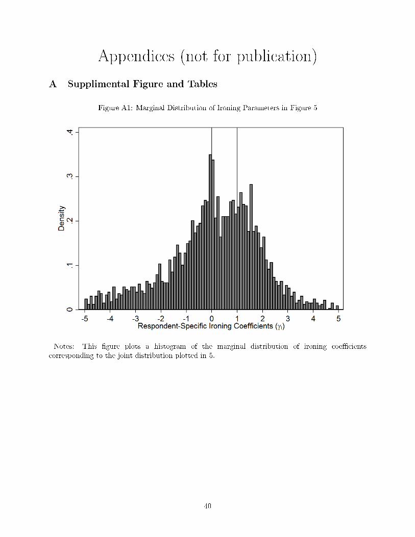
Appendices (not for publication)

A Supplimental Figure and Tables

Figure A1: Marginal Distribution of Ironing Parameters in Figure 5

Notes: This �gure plots a histogram of the marginal distribution of ironing coe�cientscorresponding to the joint distribution plotted in 5.

40

Figure A2: Marginal Distribution of Spotlighting Parameters in Figure 5

Notes: This �gure plots a histogram of the marginal distribution of spotlighting coe�cientscorresponding to the joint distribution plotted in 5.

41

Table A1: Demographics of Sample Compared to Census Data

In-sample distribution Census distribution

Gender

Male 49% 49%Female 51% 51%

Age

18-44 39% 48%45-64 44% 35%65+ 17% 17%

Income

Under $15,000 16% 12%$15,000 to $24,999 12% 10%$25,000 to $34,999 11% 10%$35,000 to $49,999 15% 13%$50,000 to $74,999 19% 17%$75,000 to $99,999 13% 12%$100,000 to $149,999 10% 14%$150,000 to $200,999 3% 6%$200,000 + 1% 6%

Notes: This table presents tabulations of the gender, age, and income distributions reported in oursample for analysis, compared against the distributions reported in the census. Age distributionscondition on being 18+.Source: http://www.census.gov/prod/cen2010/briefs/c2010br-03.pdf andhttps://www.census.gov/data/tables/2016/demo/income-poverty/p60-256.html.

42

Table A2: Parameter Estimates of Heuristic-Perception Model: Alt. Degrees of Polynomial

(1) (2) (3) (4)

γI : weight on ironing forecast 0.28*** 0.40*** 0.29*** 0.42***(0.052) (0.094) (0.052) (0.095)

γS : weight on spotlighting forecast 0.01 0.02 -0.00 -0.00(0.055) (0.075) (0.056) (0.076)

Degree of r(t) polynomial 1 1 2 2

γI : weight on ironing forecast 0.29*** 0.42*** 0.29*** 0.42***(0.052) (0.095) (0.052) (0.095)

γS : weight on spotlighting forecast -0.01 -0.01 -0.02 -0.01(0.057) (0.076) (0.057) (0.076)

Degree of r(t) polynomial 3 3 4 4

γI : weight on ironing forecast 0.29*** 0.42*** 0.30*** 0.43***(0.052) (0.095) (0.052) (0.095)

γS : weight on spotlighting forecast -0.02 -0.01 -0.02 -0.01(0.057) (0.076) (0.057) (0.076)

Degree of r(t) polynomial 5 5 6 6

γI : weight on ironing forecast 0.30*** 0.43*** 0.30*** 0.43***(0.052) (0.095) (0.052) (0.095)

γS : weight on spotlighting forecast -0.02 -0.01 -0.02 -0.01(0.057) (0.076) (0.057) (0.076)

Degree of r(t) polynomial 7 7 8 8

γI : weight on ironing forecast 0.30*** 0.43*** 0.30*** 0.43***(0.052) (0.095) (0.052) (0.095)

γS : weight on spotlighting forecast -0.02 -0.01 -0.02 -0.01(0.057) (0.076) (0.057) (0.076)

Degree of r(t) polynomial 9 9 10 10

High-income forecasts included No Yes No YesRespondents 4197 4197 4197 4197Forecasts 41970 58758 41970 58758

Notes: Standard errors, clustered by respondent, in parentheses. This table reproduces the estimatesfrom columns 2 and 4 of table 2, while varying the degree of the polynomial used to approximateresidual misperception. * p < 0.10, ** p < 0.05, *** p < 0.01.

43

Table A3: Classi�cation of Individuals to Ironing Parameters

Weight on Spotlighting Heuristic

0% 10% 20% 30% 40% 50% 60% 70% 80% 90% 100% Total

WeightonIroningHeuristic 0% 1407 55 35 23 20 22 16 19 17 31 41 1686

10% 58 10 7 1 2 1 3 4 1 21 0 10820% 36 11 2 4 3 3 0 3 12 0 0 7430% 39 6 2 1 3 2 3 19 0 0 0 7540% 38 12 4 1 1 4 21 0 0 0 0 8150% 20 8 4 5 2 28 0 0 0 0 0 6760% 27 16 5 7 24 0 0 0 0 0 0 7970% 36 13 13 35 0 0 0 0 0 0 0 9780% 29 18 59 0 0 0 0 0 0 0 0 10690% 34 91 0 0 0 0 0 0 0 0 0 125100% 1054 0 0 0 0 0 0 0 0 0 0 1054Total 2778 240 131 77 55 60 43 45 30 52 41 3552

Notes: This table presents the distribution of individual-level classi�cations of heuristic-use pa-rameters for all respondents with positive tax liability. For each respondent, we compared their10 primary-sample tax forecasts to the forecast of the model ˜Tf,i = (1 − γI − γS)T (zf,i|θi) +γI T̃I(zf,i|z∗i , θi)+γST̃S(zf,i|z∗i , θi)+ εf,i. We calculated this forecast for the grid of values of (γI , γS)indicated in the table above, and assigned each respondent to the parameter values which minimizedthe mean squared error of the di�erence.

44

Table A4: Classi�cation of Individuals to Ironing Parameters

Weight on Spotlighting Heuristic

0% 10% 20% 30% 40% 50% 60% 70% 80% 90% 100% Total

WeightonIroningHeuristic 0% 1101 84 72 70 77 56 42 26 14 24 28 1594

10% 28 13 13 11 4 8 6 8 5 10 0 10620% 26 11 5 13 7 6 10 7 12 0 0 9730% 30 8 11 4 9 2 6 18 0 0 0 8840% 24 19 9 8 7 8 15 0 0 0 0 9050% 25 16 13 9 11 29 0 0 0 0 0 10360% 34 19 17 10 28 0 0 0 0 0 0 10870% 36 24 19 45 0 0 0 0 0 0 0 12480% 39 21 68 0 0 0 0 0 0 0 0 12890% 49 88 0 0 0 0 0 0 0 0 0 137100% 977 0 0 0 0 0 0 0 0 0 0 977Total 2369 303 227 170 143 109 79 59 31 34 28 3552

Notes: This table presents the distribution of individual-level classi�cations of heuristic-use pa-rameters for all respondents with positive tax liability. For each respondent, we compared their10 primary-sample tax forecasts to the forecast of the model ˜Tf,i = (1 − γI − γS)(T (zf,i|θi) +r̂(T (zf,i|θi))) + γI T̃I(zf,i|z∗i , θi) + γST̃S(zf,i|z∗i , θi) + εf,i, where r̂ represents the �tted residual mis-perception function estimated in column 2 of table 2. We calculated this forecast for the grid ofvalues of (γI , γS) indicated in the table above, and assigned each respondent to the parameter valueswhich minimized the mean squared error of the di�erence.

45

Table A5: Classi�cation of Individuals to Ironing Parameters

Weight on Spotlighting Heuristic

0% 10% 20% 30% 40% 50% 60% 70% 80% 90% 100% Total

WeightonIroningHeuristic 0% 1134 94 44 39 42 30 29 17 26 12 20 1487

10% 26 17 11 8 11 10 4 7 9 9 0 11220% 31 14 6 8 6 1 5 7 9 0 0 8730% 31 11 7 3 2 3 2 19 0 0 0 7840% 33 11 8 5 3 4 22 0 0 0 0 8650% 26 16 14 8 7 17 0 0 0 0 0 8860% 28 20 13 7 25 0 0 0 0 0 0 9370% 40 30 18 25 0 0 0 0 0 0 0 11380% 42 30 57 0 0 0 0 0 0 0 0 12990% 57 79 0 0 0 0 0 0 0 0 0 136100% 1143 0 0 0 0 0 0 0 0 0 0 1143Total 2591 322 178 103 96 65 62 50 44 21 20 3552

Notes: This table presents the distribution of individual-level classi�cations of heuristic-use param-eters for all respondents with positive tax liability. For each respondent, we compared their 14 taxforecasts to the forecast of the model ˜Tf,i = (1−γI−γS)(T (zf,i|θi)+r̂(T (zf,i|θi)))+γI T̃I(zf,i|z∗i , θi)+γST̃S(zf,i|z∗i , θi) + εf,i, where r̂ represents the �tted residual misperception function estimated incolumn 4 of table 2. We calculated this forecast for the grid of values of (γI , γS) indicated inthe table above, and assigned each respondent to the parameter values which minimized the meansquared error of the di�erence.

46

Table A6: Parameter Estimates of Heuristic-Perception Model: Robustness to Employment Status

Restricted to unemployed respondents

γI : weight on ironing forecast 0.25∗∗∗ 0.31∗∗∗ 0.54∗∗∗ 0.53∗∗∗

(0.064) (0.090) (0.073) (0.136)

γS : weight on spotlighting forecast -0.11 -0.06 -0.12 -0.13(0.089) (0.098) (0.093) (0.110)

Residual misperception function included No Yes No YesHigh-income forecasts included No No Yes YesRespondents 1685 1685 1685 1685Forecasts 16850 16850 23590 23590

Restricted to employed respondents

γI : weight on ironing forecast 0.18∗∗∗ 0.28∗∗∗ 0.39∗∗∗ 0.34∗∗∗

(0.045) (0.065) (0.063) (0.130)

γS : weight on spotlighting forecast -0.10∗ 0.01 0.04 0.07(0.056) (0.068) (0.083) (0.105)

Residual misperception function included No Yes No YesHigh-income forecasts included No No Yes YesRespondents 2512 2512 2512 2512Forecasts 25120 25120 35168 35168

Notes: Standard errors, clustered by respondent, in parentheses. This table reproduces the analysisof table 2, restricting the sample to employed or unemployed respondents. * p < 0.10, ** p < 0.05,*** p < 0.01.

47

Table A7: Parameter Estimates of Heuristic-Perception Model: Robustness to Who Completed TaxReturn

Restricted to respondents who completed their own tax return

γI : weight on ironing forecast 0.12∗∗ 0.20∗∗∗ 0.34∗∗∗ 0.30∗∗

(0.050) (0.066) (0.061) (0.124)

γS : weight on spotlighting forecast -0.04 0.03 0.06 0.08(0.065) (0.073) (0.077) (0.098)

Residual misperception function included No Yes No YesHigh-income forecasts included No No Yes YesRespondents 2301 2301 2301 2301Forecasts 23010 23010 32214 32214

Restricted to respondents who did not complete their own tax return

(1) (2) (3) (4)

γI : weight on ironing forecast 0.31∗∗∗ 0.39∗∗∗ 0.57∗∗∗ 0.57∗∗∗

(0.054) (0.081) (0.077) (0.144)

γS : weight on spotlighting forecast -0.15∗ -0.05 -0.12 -0.12(0.077) (0.089) (0.102) (0.120)

Residual misperception function included No Yes No YesHigh-income forecasts included No No Yes YesRespondents 1896 1896 1896 1896Forecasts 18960 18960 26544 26544

Notes: Standard errors, clustered by respondent, in parentheses. This table reproduces the analysisof table 2, restricting the sample to respondents who did, or did not, complete their own tax return.* p < 0.10, ** p < 0.05, *** p < 0.01.

48

Table A8: Parameter Estimates of Heuristic-Perception Model: Robustness to Use of Tax Prepara-tion Software

Restricted to respondents who used tax preparation software

γI : weight on ironing forecast 0.19∗∗∗ 0.28∗∗∗ 0.36∗∗∗ 0.41∗∗∗

(0.052) (0.075) (0.064) (0.135)

γS : weight on spotlighting forecast -0.07 0.00 0.08 0.05(0.064) (0.075) (0.081) (0.105)

Residual misperception function included No Yes No YesHigh-income forecasts included No No Yes YesRespondents 2242 2242 2242 2242Forecasts 22420 22420 31388 31388

Restricted to respondents who did not use tax preparation software

(1) (2) (3) (4)

γI : weight on ironing forecast 0.20∗∗∗ 0.31∗∗∗ 0.50∗∗∗ 0.42∗∗∗

(0.055) (0.074) (0.079) (0.144)

γS : weight on spotlighting forecast -0.08 0.02 -0.08 -0.06(0.075) (0.085) (0.104) (0.121)

Residual misperception function included No Yes No YesHigh-income forecasts included No No Yes YesRespondents 1590 1590 1590 1590Forecasts 15900 15900 22260 22260

Notes: Standard errors, clustered by respondent, in parentheses. This table reproduces the analysisof table 2, restricting the sample to respondents who did, or did not, use tax preparation software.365 respondents who did not know if tax preparation software was used are excluded. * p < 0.10,** p < 0.05, *** p < 0.01.

49

Table A9: Parameter Estimates of Heuristic-Perception Model: Di�erences by Survey Date

Restricted to responses on or before tax day

(1) (2) (3) (4)

γI : weight on ironing forecast 0.23∗∗∗ 0.30∗∗∗ 0.40∗∗∗ 0.33∗∗

(0.054) (0.075) (0.073) (0.134)

γS : weight on spotlighting forecast -0.06 0.03 0.08 0.12(0.074) (0.086) (0.094) (0.112)

Residual misperception function included No Yes No YesHigh-income forecasts included No No Yes YesRespondents 2080 2080 2080 2080Forecasts 20800 20800 29120 29120

Restricted to responses after tax day

(1) (2) (3) (4)

γI : weight on ironing forecast 0.19∗∗∗ 0.29∗∗∗ 0.48∗∗∗ 0.52∗∗∗

(0.051) (0.071) (0.063) (0.135)

γS : weight on spotlighting forecast -0.12∗ -0.05 -0.11 -0.13(0.067) (0.076) (0.082) (0.104)

Residual misperception function included No Yes No YesHigh-income forecasts included No No Yes YesRespondents 2117 2117 2117 2117Forecasts 21170 21170 29638 29638

Notes: Standard errors, clustered by respondent, in parentheses. This table reproduces the analysisof table 2, restricting the sample by the time period when the respondent completed the survey. *p < 0.10, ** p < 0.05, *** p < 0.01.

50

Table A10: Parameter Estimates of Heuristic-Perception Model: Di�erences by Financial Literacy

Restricted to �nancially literate respondents

(1) (2) (3) (4)

γI : weight on ironing forecast 0.02 0.26∗∗∗ 0.18∗∗∗ 0.34∗∗∗

(0.040) (0.059) (0.060) (0.108)

γS : weight on spotlighting forecast -0.11∗∗ -0.02 0.12 0.03(0.049) (0.061) (0.082) (0.095)

Residual misperception function included No Yes No YesHigh-income forecasts included No No Yes YesRespondents 1899 1899 1899 1899Forecasts 18990 18990 26586 26586

Restricted to �nancially illiterate respondents

(1) (2) (3) (4)

γI : weight on ironing forecast 0.39∗∗∗ 0.23∗∗∗ 0.76∗∗∗ 0.36∗∗

(0.062) (0.087) (0.073) (0.150)

γS : weight on spotlighting forecast -0.18∗∗ -0.06 -0.28∗∗∗ -0.08(0.083) (0.091) (0.091) (0.114)

Residual misperception function included No Yes No YesHigh-income forecasts included No No Yes YesRespondents 2298 2298 2298 2298Forecasts 22980 22980 32172 32172

Notes: Standard errors, clustered by respondent, in parentheses. This table reproduces the analysisof table 2, restricting the sample by respondents' �nancial literacy classi�cation. Respondentsare coded if they answered all of the Lusardi and Mitchell �Big Three� �nancial literacy questionscorrectly; otherwise, they are classi�ed as �nancially illiterate. * p < 0.10, ** p < 0.05, *** p < 0.01.

51

Table A11: Welfare Analysis of Debiasing Policy: Simulation with Alternative CRRA Utility

Panel A: CRRA parameter = 0.5

Elasticity Lost Govt. Net Welfare Loss (%)

Parameter Revenue (%) Low λ � High λ(k) λ = U ′10 λ = U ′50 λ = U ′90

Elasticity→ 1 4.4 4.1 4.2 4.3

2 2.3 2.2 2.2 2.33 1.6 1.5 1.5 1.54 1.2 1.1 1.1 1.25 1.0 0.9 0.9 0.9

Panel B: CRRA parameter = 2

Elasticity Lost Govt. Net Welfare Loss (%)

Parameter Revenue (%) Low λ � High λ(k) λ = U ′10 λ = U ′50 λ = U ′90

Elasticity→ 1 4.4 4.0 4.4 4.4

2 2.3 2.1 2.3 2.33 1.6 1.4 1.5 1.64 1.2 1.1 1.1 1.25 1.0 0.9 0.9 1.0

Notes: This table reproduces the analysis of table 4, but generalizes the ln utility component toCRRA preferences of di�ering parameters governing redistributive preferences.

52

Table A12: Welfare Analysis of Debiasing Policy: Simulation with Locally Estimated Misperceptions

Panel A: Applying Full-Sample Estimate

Elasticity Lost Govt. Net Welfare Loss (%)

Parameter Revenue (%) Low λ � High λ(k) λ = U ′10 λ = U ′50 λ = U ′90

Elasticity→ 1 8.2 7.1 7.8 8.0

2 4.3 3.8 4.0 4.23 2.9 2.6 2.8 2.94 2.2 1.9 2.1 2.25 1.8 1.6 1.7 1.8

Panel B: Applying Quartile-Speci�c Estimates

Elasticity Lost Govt. Net Welfare Loss (%)

Parameter Revenue (%) Low λ � High λ(k) λ = U ′10 λ = U ′50 λ = U ′90

Elasticity→ 1 7.8 6.8 7.4 7.7

2 4.1 3.6 3.9 4.13 2.8 2.5 2.7 2.84 2.1 1.9 2.0 2.15 1.7 1.5 1.6 1.7

Notes: This table reproduces the analysis of table 4, but assumes that taxpayers apply the locallyestimated �attening parameter (bottom panel of table 1) rather than the heuristic forecasting model.The top panel applies the estimate of column 1, and the bottom panel applies the quartile-speci�cestimates of columns 2-5.

53

B In�uence of the Inclusion of Additional Taxes

Figure B1: Estimates of Residual Tax Misperception: Assuming Respondents Included FICA Taxin Forecasts

Notes: This �gure plots the residual misperception functions estimated in columns 2 and 4 of tableB1.

54

Figure B2: Estimates of Residual Tax Misperception: Assuming Respondents Included State Taxin Forecasts

Notes: This �gure plots the residual misperception functions estimated in columns 2 and 4 of tableB2.

55

Figure B3: Estimates of Residual Tax Misperception: Assuming Respondents Included State andFICA Tax in Forecasts

Notes: This �gure plots the residual misperception functions estimated in columns 2 and 4 of tableB3.

56

Table B1: Parameter Estimates of Heuristic-Perception Model: Assuming Respondents IncludedFICA Tax in Forecasts

(1) (2) (3) (4)

γI : weight on ironing forecast 0.88∗∗∗ 0.32∗∗∗ 1.04∗∗∗ 0.55∗∗∗

(0.046) (0.065) (0.048) (0.098)

γS : weight on spotlighting forecast -0.24∗∗∗ -0.03 -0.38∗∗∗ -0.12(0.063) (0.072) (0.065) (0.081)

Residual misperception function included? No Yes No YesHigh-income forecasts included No No Yes YesRespondents 4197 4197 4197 4197Forecasts 41970 41970 58758 58758

Notes: Standard errors, clustered by respondent, in parentheses. This table reproduces the estimatesof table 2, but calculates the true tax, ATR, and MTR to include FICA taxes. Estimated residualmisperception functions are plotted in Appendix Figure B1. * p < 0.10, ** p < 0.05, *** p < 0.01.

57

Table B2: Parameter Estimates of Heuristic-Perception Model: Assuming Respondents IncludedState Tax in Forecasts

(1) (2) (3) (4)

γI : weight on ironing forecast 0.48∗∗∗ 0.22∗∗∗ 0.78∗∗∗ 0.35∗∗∗

(0.032) (0.045) (0.040) (0.077)

γS : weight on spotlighting forecast -0.16∗∗∗ -0.02 -0.28∗∗∗ -0.05(0.044) (0.051) (0.052) (0.065)

Residual misperception function included? No Yes No YesHigh-income forecasts included No No Yes YesRespondents 4163 4163 4163 4163Forecasts 41630 41630 58282 58282

Notes: Standard errors, clustered by respondent, in parentheses. This table reproduces the estimatesof table 2, but calculates the true tax, ATR, and MTR to include State taxes. Estimated residualmisperception functions are plotted in Appendix Figure B2. * p < 0.10, ** p < 0.05, *** p < 0.01.

58

Table B3: Parameter Estimates of Heuristic-Perception Model: Assuming Respondents IncludedState and FICA Tax in Forecasts

(1) (2) (3) (4)

γI : weight on ironing forecast 1.10∗∗∗ 0.24∗∗∗ 1.30∗∗∗ 0.45∗∗∗

(0.039) (0.054) (0.039) (0.079)

γS : weight on spotlighting forecast -0.38∗∗∗ -0.03 -0.60∗∗∗ -0.13∗

(0.054) (0.061) (0.053) (0.067)

Residual misperception function included? No Yes No YesHigh-income forecasts included No No Yes YesRespondents 4163 4163 4163 4163Forecasts 41630 41630 58282 58282

Notes: Standard errors, clustered by respondent, in parentheses. This table reproduces the estimatesof table 2, but calculates the true tax, ATR, and MTR to include both State and FICA taxes.Estimated residual misperception functions are plotted in Appendix Figure B3. * p < 0.10, **p < 0.05, *** p < 0.01.

59

Table B4: Welfare Analysis of Debiasing Policy

Panel A: State + FICA Taxes Perfectly Perceived Before and After Nudge

Elasticity Lost Govt. Net Welfare Loss (%)

Parameter Revenue (%) Low λ � High λ(k) λ = U ′10 λ = U ′50 λ = U ′90

Elasticity→ 1 4.9 4.6 4.8 4.9

2 2.6 2.4 2.5 2.63 1.8 1.7 1.7 1.74 1.3 1.3 1.3 1.35 1.0 1.0 1.1 1.1

Panel B: State + FICA Taxes Ignored Before Nudge, Perfectly Perceived After

Elasticity Lost Govt. Net Welfare Loss (%)

Parameter Revenue (%) Low λ � High λ(k) λ = U ′10 λ = U ′50 λ = U ′90

Elasticity→ 1 22.7 9.1 16.9 21.5

2 12.8 5.6 9.7 12.13 8.9 4.0 6.8 8.54 6.8 3.1 5.2 6.45 5.5 2.5 4.3 5.2

Notes: This table reproduces the analysis of table 4 under two alternative treatments of Stateand FICA taxes. In both panels, we include both State taxes and FICA taxes when calculatingthe actual tax burden, although we model these as externally imposed taxes, with revenue notcontrolled by our social planner. In the simulations reported in the top panel, we assume thattaxpayers correctly perceive State and FICA taxes both before and after the nudge: prior to thenudge, tax misperceptions are limited to the federal income tax. In the simulations reported in thebottom panel, we assume that taxpayers completely ignore State and FICA taxes before the nudge,but correctly account for them after the nudge.

60

C In�uence of Similarity to Fred

Figure C1: Estimates of Residual Tax Misperception: Respondents with Simple Tax Returns

Notes: This �gure plots the residual misperception functions estimated in columns 2 and 4 of thetop panel of table C3.

61

Figure C2: Estimates of Residual Tax Misperception: Respondents with Complex Tax Returns

Notes: This �gure plots the residual misperception functions estimated in columns 2 and 4 of thebottom panel of table C3.

62

Table C1: Testing for �Flattening� of the Tax Schedule: Robustness to Similarity with HypotheticalFiler (Similar Filers)

All Incomes Income QuartilesPooled 1 2 3 4

Estimation sample: Primary and High-Income Sampling Distributions

Scale of slope (β) 0.56*** 0.52*** 0.53*** 0.58*** 0.74***(0.018) (0.030) (0.032) (0.039) (0.057)

P-value of H0: β = 1 0.000 0.000 0.000 0.000 0.000Respondents 1357 441 446 322 148Forecasts 18998 6174 6244 4508 2072

Estimation sample: Primary Sampling Distribution

Scale of slope (β) 0.77*** 0.72*** 0.76*** 0.74*** 0.93***(0.027) (0.049) (0.050) (0.054) (0.072)

P-value of H0: β = 1 0.000 0.000 0.000 0.000 0.301Respondents 1357 441 446 322 148Forecasts 13570 4410 4460 3220 1480

Estimation sample: Local Draws

Scale of slope (β) 0.78*** 0.99*** 1.11*** 0.82*** 0.70***(0.077) (0.166) (0.200) (0.084) (0.130)

P-value of H0: β = 1 0.005 0.970 0.596 0.028 0.022Respondents 1357 441 446 322 148Forecasts 5489 1318 1749 1634 788

Notes: Standard errors, clustered by respondent, in parentheses. Presented are coe�cients fromOLS �xed-e�ect regressions of the form T̃i,f = β∗Ti,f+γi+εi,f . The coe�cient β can be interpretedas a scaling of the slope induced by the true tax schedule, where estimated values less than 1 indicatea ��attening� of the tax schedule. Two-sided Wald-test p-values, testing the hypothesis that β = 1,are presented below each regression. * p < 0.10, ** p < 0.05, *** p < 0.01.

63

Table C2: Testing for �Flattening� of the Tax Schedule: Robustness to Similarity with HypotheticalFiler (Dissimilar Filers)

All Incomes Income QuartilesPooled 1 2 3 4

Estimation sample: Primary and High-Income Sampling Distributions

Scale of slope (β) 0.66*** 0.58*** 0.57*** 0.63*** 0.78***(0.012) (0.028) (0.028) (0.021) (0.018)

P-value of H0: β = 1 0.000 0.000 0.000 0.000 0.000Respondents 2840 561 620 738 921Forecasts 39760 7854 8680 10332 12894

Estimation sample: Primary Sampling Distribution

Scale of slope (β) 0.84*** 0.71*** 0.78*** 0.82*** 0.94***(0.015) (0.038) (0.037) (0.028) (0.024)

P-value of H0: β = 1 0.000 0.000 0.000 0.000 0.010Respondents 2840 561 620 738 921Forecasts 28400 5610 6200 7380 9210

Estimation sample: Local Draws

Scale of slope (β) 0.81*** 1.18** 1.11*** 0.85*** 0.80***(0.049) (0.578) (0.137) (0.075) (0.058)

P-value of H0: β = 1 0.000 0.757 0.408 0.040 0.000Respondents 2840 561 620 738 921Forecasts 12449 1660 2293 3737 4759

Notes: Standard errors, clustered by respondent, in parentheses. Presented are coe�cients fromOLS �xed-e�ect regressions of the form T̃i,f = β∗Ti,f+γi+εi,f . The coe�cient β can be interpretedas a scaling of the slope induced by the true tax schedule, where estimated values less than 1 indicatea ��attening� of the tax schedule. Two-sided Wald-test p-values, testing the hypothesis that β = 1,are presented below each regression. * p < 0.10, ** p < 0.05, *** p < 0.01.

64

Table C3: Parameter Estimates of Heuristic-Perception Model: Robustness to Similarity with Hy-pothetical Filer

Restricted to respondents with simple tax returns

γI : weight on ironing forecast 0.29*** 0.46*** 0.61*** 0.56***(0.098) (0.145) (0.104) (0.210)

γS : weight on spotlighting forecast -0.18 -0.21 -0.17 -0.17(0.147) (0.153) (0.133) (0.156)

Residual misperception function included No Yes No YesHigh-income forecasts included No No Yes YesRespondents 1357 1357 1357 1357Forecasts 13570 13570 18998 18998

Restricted to respondents with complex tax returns

γI : weight on ironing forecast 0.18*** 0.23*** 0.39*** 0.33***(0.040) (0.059) (0.053) (0.110)

γS : weight on spotlighting forecast -0.08 0.05 0.02 0.05(0.048) (0.058) (0.069) (0.088)

Residual misperception function included No Yes No YesHigh-income forecasts included No No Yes YesRespondents 2840 2840 2840 2840Forecasts 28400 28400 39760 39760

Notes: Standard errors, clustered by respondent, in parentheses. This table reproduces the analysisof table 2, restricting the sample to respondents who do (or do not) have the same simple tax �lingbehavior that was speci�ed in our scenarios. Estimated residual misperception functions are plottedin appendix tables C1 and C2. * p < 0.10, ** p < 0.05, *** p < 0.01.

65

D Robustness to Data Cleaning Decisions

Table D1: Testing for �Flattening� of the Tax Schedule: Including Respondents Who Failed Atten-tion Check

All Incomes Income QuartilesPooled 1 2 3 4

Estimation Sample: Primary and High-Income Sampling Distributions

Scale of slope (β) 0.61*** 0.52*** 0.55*** 0.61*** 0.76***(0.010) (0.019) (0.020) (0.019) (0.017)

P-value of H0: β = 1 0.000 0.000 0.000 0.000 0.000Respondents 4633 1159 1167 1149 1158Forecasts 64862 16226 16338 16086 16212

Estimation Sample: Primary Sampling Distribution

Scale of slope (β) 0.81*** 0.69*** 0.76*** 0.79*** 0.93***(0.013) (0.029) (0.030) (0.026) (0.023)

P-value of H0: β = 1 0.000 0.000 0.000 0.000 0.003Respondents 4633 1159 1167 1149 1158Forecasts 46330 11590 11670 11490 11580

Estimation Sample: Local Draws

Scale of slope (β) 0.84*** 0.99*** 1.09*** 0.82*** 0.84***(0.065) (0.221) (0.110) (0.056) (0.084)

P-value of H0: β = 1 0.016 0.977 0.424 0.002 0.051Respondents 4633 1159 1167 1149 1158Forecasts 19675 3436 4419 5788 6032

Notes: Standard errors, clustered by respondent, in parentheses. Presented are coe�cients fromOLS �xed-e�ect regressions of the form T̃i,f = β∗Ti,f+γi+εi,f . The coe�cient β can be interpretedas a scaling of the slope induced by the true tax schedule, where estimated values less than 1 indicatea ��attening� of the tax schedule. Two-sided Wald-test p-values, testing the hypothesis that β = 1,are presented below each regression. * p < 0.10, ** p < 0.05, *** p < 0.01.

66

Table D2: Parameter Estimates of Heuristic-Perception Model: Including Respondents Who FailedAttention Check

(1) (2) (3) (4)

γI : weight on ironing forecast 0.21*** 0.29*** 0.44*** 0.39***(0.040) (0.056) (0.047) (0.094)

γS : weight on spotlighting forecast -0.09* 0.00 0.01 0.04(0.051) (0.058) (0.059) (0.074)

Residual misperception function included No Yes No YesHigh-income forecasts included No No Yes YesRespondents 4633 4633 4633 4633Forecasts 46330 46330 64862 64862

Notes: Standard errors, clustered by respondent, in parentheses. This table reproduces the estimatesof table 2 after including subjects who failed the attention check in the estimation sample.* p < 0.10,** p < 0.05, *** p < 0.01.

67

Table D3: Testing for �Flattening� of the Tax Schedule: Winsorized at 5pct and 95pct forecastvalues

All Incomes Income QuartilesPooled 1 2 3 4

Estimation Sample: Primary and High-Income Sampling Distributions

Scale of slope (β) 0.59*** 0.50*** 0.51*** 0.58*** 0.75***(0.008) (0.016) (0.015) (0.015) (0.015)

P-value of H0: β = 1 0.000 0.000 0.000 0.000 0.000Respondents 4197 1002 1066 1060 1069Forecasts 58758 14028 14924 14840 14966

Estimation Sample: Primary Sampling Distribution

Scale of slope (β) 0.77*** 0.64*** 0.69*** 0.75*** 0.91***(0.010) (0.021) (0.021) (0.020) (0.018)

P-value of H0: β = 1 0.000 0.000 0.000 0.000 0.000Respondents 4197 1002 1066 1060 1069Forecasts 41970 10020 10660 10600 10690

Estimation Sample: Local Draws

Scale of slope (β) 0.76*** 0.82*** 1.01*** 0.81*** 0.74***(0.035) (0.084) (0.071) (0.033) (0.045)

P-value of H0: β = 1 0.000 0.032 0.919 0.000 0.000Respondents 4197 1002 1066 1060 1069Forecasts 17938 2978 4042 5371 5547

Notes: Standard errors, clustered by respondent, in parentheses. Presented are coe�cients fromOLS �xed-e�ect regressions of the form T̃i,f = β∗Ti,f+γi+εi,f . The coe�cient β can be interpretedas a scaling of the slope induced by the true tax schedule, where estimated values less than 1 indicatea ��attening� of the tax schedule. Two-sided Wald-test p-values, testing the hypothesis that β = 1,are presented below each regression. * p < 0.10, ** p < 0.05, *** p < 0.01.

68

Table D4: Testing for �Flattening� of the Tax Schedule: Winsorized to 0-100% tax rates

All Incomes Income QuartilesPooled 1 2 3 4

Estimation Sample: Primary and High-Income Sampling Distributions

Scale of slope (β) 0.63*** 0.56*** 0.55*** 0.62*** 0.78***(0.010) (0.021) (0.020) (0.019) (0.017)

P-value of H0: β = 1 0.000 0.000 0.000 0.000 0.000Respondents 4197 1002 1066 1060 1069Forecasts 58758 14028 14924 14840 14966

Estimation Sample: Primary Sampling Distribution

Scale of slope (β) 0.83*** 0.72*** 0.78*** 0.80*** 0.95***(0.013) (0.030) (0.030) (0.026) (0.022)

P-value of H0: β = 1 0.000 0.000 0.000 0.000 0.021Respondents 4197 1002 1066 1060 1069Forecasts 41970 10020 10660 10600 10690

Estimation Sample: Local Draws

Scale of slope (β) 0.82*** 1.10*** 1.13*** 0.84*** 0.79***(0.044) (0.230) (0.113) (0.055) (0.056)

P-value of H0: β = 1 0.000 0.677 0.268 0.005 0.000Respondents 4197 1002 1066 1060 1069Forecasts 17938 2978 4042 5371 5547

Notes: Standard errors, clustered by respondent, in parentheses. Presented are coe�cients fromOLS �xed-e�ect regressions of the form T̃i,f = β∗Ti,f+γi+εi,f . The coe�cient β can be interpretedas a scaling of the slope induced by the true tax schedule, where estimated values less than 1 indicatea ��attening� of the tax schedule. Two-sided Wald-test p-values, testing the hypothesis that β = 1,are presented below each regression. * p < 0.10, ** p < 0.05, *** p < 0.01.

69

Table D5: Testing for �Flattening� of the Tax Schedule: No Winsorization

All Incomes Income QuartilesPooled 1 2 3 4

Estimation Sample: Primary and High-Income Sampling Distributions

Scale of slope (β) 0.67*** 0.56*** 0.58*** 0.69*** 0.84***(0.027) (0.033) (0.034) (0.086) (0.042)

P-value of H0: β = 1 0.000 0.000 0.000 0.000 0.000Respondents 4197 1002 1066 1060 1069Forecasts 58758 14028 14924 14840 14966

Estimation Sample: Primary Sampling Distribution

(1) (2) (3) (4) (5)

Scale of slope (β) 0.88*** 0.74*** 1.06*** 0.76*** 0.94***(0.058) (0.131) (0.215) (0.047) (0.026)

P-value of H0: β = 1 0.043 0.048 0.776 0.000 0.020Respondents 4197 1002 1066 1060 1069Forecasts 41970 10020 10660 10600 10690

Estimation Sample: Local Draws

Scale of slope (β) 0.44 1.65*** 0.86** -0.19 0.60**(0.318) (0.593) (0.429) (1.200) (0.250)

P-value of H0: β = 1 0.081 0.270 0.744 0.323 0.109Respondents 4197 1002 1066 1060 1069Forecasts 17938 2978 4042 5371 5547

Notes: Standard errors, clustered by respondent, in parentheses. Presented are coe�cients fromOLS �xed-e�ect regressions of the form T̃i,f = β∗Ti,f+γi+εi,f . The coe�cient β can be interpretedas a scaling of the slope induced by the true tax schedule, where estimated values less than 1 indicatea ��attening� of the tax schedule. Two-sided Wald-test p-values, testing the hypothesis that β = 1,are presented below each regression. * p < 0.10, ** p < 0.05, *** p < 0.01.

70

Table D6: Parameter Estimates of Heuristic-Perception Model: Alt. Winsorizations

Winsorized at the 5th and 90th percentile forecast

γI : weight on ironing forecast 0.30*** 0.32*** 0.54*** 0.46***(0.027) (0.041) (0.036) (0.072)

γS : weight on spotlighting forecast -0.06* 0.00 -0.06 -0.02(0.033) (0.039) (0.046) (0.057)

Winsorized at 0% and 100% of income

γI : weight on ironing forecast 0.20*** 0.29*** 0.45*** 0.43***(0.037) (0.052) (0.047) (0.092)

γS : weight on spotlighting forecast -0.08 -0.01 -0.02 -0.02(0.050) (0.057) (0.062) (0.075)

No Winsorization

γI : weight on ironing forecast 0.06 0.27 0.30*** 0.56**(0.119) (0.245) (0.083) (0.234)

γS : weight on spotlighting forecast -0.15 -0.02 0.08 -0.06(0.146) (0.214) (0.099) (0.148)

Residual misperception function included No Yes No YesHigh-income forecasts included No No Yes YesRespondents 4197 4197 4197 4197Forecasts 41970 41970 58758 58758

Notes: Standard errors, clustered by respondent, in parentheses. This table reproduces theanalysis of table 2 under alternative treatments of outliers. * p < 0.10, ** p < 0.05, *** p < 0.01.

E Proofs

Proof of Proposition 1 Assume that G(u) = u; which is without loss of generality since monotonic

transformations of utility functions preserve behaviors.

Part 1. Let Bw(z′) denote the optimal choice of z by an individual facing tax schedule T̃ (z|z′). Note

the following:

1. Bw(z′) is uniquely de�ned since T̃ (z|z′) is convex. The convexity of T̃ (z|·) follows by assumption A

combined with the assumption that T (z) is convex.

2. Bw(z′) is guaranteed to be continuous in z′ because T̃ (z|z′) is continuous in z′ and (c−ψ(z/w))−T̃ (z|z′)

is strictly concave in z.

3. Bw(z′) is decreasing in z′. This is because assumption A and the assumption that T (z) is convex

guarantee that the perceived marginal tax rates are increasing in z′.

4. Bw(0) > 0, since the assumption that ψ(0) = 0 guarantees that the optimal choice of z is interior for any

perceived tax schedule. Also, Bw(z′) < z′ for large enough z′ by the assumption that limz→∞ ψ′(z) =

∞.

71

The above four facts show that Bw(z′) is a continuous and decreasing function with Bw(0) > 0 and Bw(z) < z

for large enough z. A basic application of the intermediate value theorem establishes that this function must

intersect the 45-degree line exactly once.

Part 2. Continuity follows immediately since c−ψ(z/w)− T̃ (z|z′) is continuous w and is strictly concave

in z. Next, note that for any z1 > z2 and z′,(c− ψ(z1/w)− T̃ (z1|z′)

)−(c− ψ(z2/w)− T̃ (z2|z′)

)is strictly

increasing in w because ψ is convex. The statement in the proposition is thus a standard comparative static

on �xed points (see, e.g., Villas-Boas, 2016). Moreover, z∗ will be strictly increasing in w if it is interior.

Part 3. Continuity follows immediately since T̃ is continuous in γI and γr, and since c−ψ(z/w)− T̃ (z|z′)is strictly concave in z. Next, it follows immediately by assumption A that for z1 > z2, T (z1|z′)−T (z2|z′) isdecreasing in γI and γr. Thus, for any z1 > z2 and z

′,(c− ψ(z1/w)− T̃ (z1|z′)

)−(c− ψ(z2/w)− T̃ (z2|z′)

)is strictly increasing in γI and γr. The result then follows as in Part 2. �

An observation: It is useful to note that convexity of T plays two important roles in the proof of

Proposition 1. First, it ensures that the individual's optimization problem is convex, and thus that Bw is

single-valued. In particular, this then ensures that Bw has a closed graph, a property that would not hold

for all possible T . Second, convexity of T ensures that Bw is a decreasing function. If T were concave,

however, Bw would be an increasing function; and more generally, Bw could be increasing in some regions

and decreasing in others for some tax schedules T . Existence and uniqueness are thus not guaranteed for all

possible T . To ensure existence, the ME concept would need to be extended to allow for �mixed strategies.�

Proof of Proposition 2 We denote by d+z∗

dγI:= limε→0

z∗(γI+|ε|)−z∗(γI)|ε| the right derivative. We prove

proposition 2 without assuming that T is not everywhere di�erentiable�that is, we allow T to have kink

points. We only make the assumption that the distribution w of types is smooth, and thus that not all

consumers are at kink points.

We show that ddγ I

W |γI=0,γr=0 > 0, from which the result follows. Let τ̃w(z) < T ′(z∗(w)) denote the

individual's perceived marginal tax rate. By de�nition, 1− ψ′/w = τ̃w.

=

�G′ · (1− ψ′/w − T ′)d+z

∗

dγIdF + λ

�d+z

∗

dγIT ′dF

=

�G′ · (τ̃w − T ′)dF + λ

�d+z

∗

dγIT ′dF

Now when γI = γr = 0, τ̃w = T ′ for all w; that is, consumers perceive tax rates correctly by de�nition.

Thus ddγ I

W |γI=0,γr=0 = λ� d+z

∗

dγIT ′dF . The result follows by part 3 of proposition 1, which shows that

earnings are increasing in γI , and are strictly increasing for consumers who are not at kink points, and thusd+z

∗

dγI> 0 for a positive measure of consumers.�

Proof of Proposition 3. More generally, we prove the results by replacing dz∗

dn with d+z∗

dn in part 1,

and replacing it with d−z∗

dn in part 2. To keep the proof concise we abuse notation slightly and use dz∗

dn to

denote the appropriate left or right derivative.

Analogously to the proof of Proposition 2, we can write

72

d

dnW /λ =

�g(z) · (1− ψ′/w − T ′)dz

∗

dndF +

�dz∗

dnT ′dF

=

�dz∗

dnT ′ (1− g(z∗)) dF +

�g(z)τ̃w

dz∗

dndF (6)

Since τ̃w ≥ 0, the term�g(z)τ̃w

dz∗

dn in equation (6) positive when dz∗

dn is positive and negative when dz∗

dn

is negative. Thus the term in equation (6) is less than (greater than)�dz∗

dn T′ (1− g(z∗)) dF when dz∗

dn is

positive (negative). Moreover, note that

�dz∗

dnT ′ (1− g(z∗)) dF = − Cov

[dz∗

dnT ′, g(z∗)

]+ E

[dz∗

dnT ′]E [1− g(z∗)]

Now Cov[dz∗

dn T′, g(z∗)

]is non-negative when dz∗

dn is decreasing in w, and is non-positive when dz∗

dn is in-

creasing in w. Similarly, E[dz∗

dn T′]E [1− g(z∗)] is non-positive (non-negative) when E[g(z∗)] ≤ 1 and dz∗

dn is

non-positive (non-negative) for all w. This proves that when∣∣∣dz∗dn ∣∣∣ is increasing in w, � dz∗

dn T′ (1− g(z∗)) dF

negative (positive) if dz∗

dn is negative (positive) for all w.�

73