Heuristic Optimization Methods in Econometrics∗

M. Gilli† P. Winker‡

October 21, 2007

∗We are indebted to M. Meyer, G. di Tollo, and three anonymous referees for valuablecomments on preliminary drafts. Both authors gratefully acknowledge financial support fromthe EU Commission through MRTN-CT-2006-034270 COMISEF.

†Department of Econometrics, University of Geneva and Swiss Finance Institute, Switzer-land

‡Department of Economics, University of Giessen, Germany

1

Contents

1 Traditional numerical versus heuristic optimization methods 31.1 Optimization in econometrics . . . . . . . . . . . . . . . . . . . . 31.2 Optimization heuristics . . . . . . . . . . . . . . . . . . . . . . . . 41.3 An uncomplete collection of applications . . . . . . . . . . . . . . 71.4 Structure and instructions for use of the chapter . . . . . . . . . . 8

2 Heuristic optimization 92.1 Basic concepts . . . . . . . . . . . . . . . . . . . . . . . . . . . . . 92.2 Trajectory methods . . . . . . . . . . . . . . . . . . . . . . . . . . 11

2.2.1 Threshold methods (TM) . . . . . . . . . . . . . . . . . . 112.2.2 Tabu search (TS) . . . . . . . . . . . . . . . . . . . . . . . 12

2.3 Population based methods . . . . . . . . . . . . . . . . . . . . . . 122.3.1 Genetic algorithm (GA) . . . . . . . . . . . . . . . . . . . 132.3.2 Ant colonies (AC) . . . . . . . . . . . . . . . . . . . . . . . 132.3.3 Differential evolution (DE) . . . . . . . . . . . . . . . . . . 142.3.4 Particle Swarm Optimization (PS) . . . . . . . . . . . . . 15

2.4 Hybrid meta-heuristics . . . . . . . . . . . . . . . . . . . . . . . . 162.4.1 Basic characteristics of meta-heuristics . . . . . . . . . . . 172.4.2 Scheme for possible hybridization . . . . . . . . . . . . . . 182.4.3 An example: Memetic algorithms (MA) . . . . . . . . . . . 20

3 Stochastics of the solution 213.1 Optimization as stochastic mapping . . . . . . . . . . . . . . . . . 213.2 Convergence of heuristics . . . . . . . . . . . . . . . . . . . . . . . 233.3 Convergence of optimization based estimators . . . . . . . . . . . 26

4 General guidelines for the use of optimization heuristics 274.1 Implementation . . . . . . . . . . . . . . . . . . . . . . . . . . . . 284.2 Presentation of results . . . . . . . . . . . . . . . . . . . . . . . . 34

5 Selected applications 365.1 Model selection in VAR models . . . . . . . . . . . . . . . . . . . 365.2 High breakdown point estimation . . . . . . . . . . . . . . . . . . 38

6 Conclusions 42

2

1 Traditional numerical versus heuristic

optimization methods

1.1 Optimization in econometrics

Before introducing heuristic optimization methods and providing an overviewof some applications in econometrics, we have to motivate the use of such anoptimization paradigm in econometrics. Obviously, optimization is at the core ofeconometric applications to real data sets, e.g., in model selection and parameterestimation. Consequently, econometrics is a field with a long tradition in applyingthe most up to date optimization techniques.

Maybe the most widely used technique is least squares estimation for linear mod-els. The optimization problem in this case results in a system of linear equationswhich can be solved by standard techniques from linear algebra. However, incase of ill-conditioned matrices, e.g., due to very high multicolinearity, or hugemodels, even this simple model might pose some numerical problems.

A more demanding class of optimization problems stems from general maximumlikelihood estimation. As long as the likelihood function can be considered asbeing globally convex, efficient numerical methods are available to solve the op-timization problem. However, in this class of models, the number of notoriouscases with flat likelihood functions or functions with several local optima is al-ready quite substantial. Even a conceptually simple estimation problem such asGARCH(1,1) might sometimes result in a likelihood function which does not al-low for the successful application of standard numerical approximation algorithmssuch as BHHH (Jerrell and Campione, 2001; Doornik and Ooms, 2003; Maringerand Winker, 2006). Some more examples will be discussed at the end of thissection and in Section 5 together with the application of optimization heuristics.

Furthermore, there exist problem instances, e.g., in model selection, where tra-ditional numerical methods cannot be applied at all due to the discretenessof the search space (Winker, 2000; Winker and Maringer, 2004; Maringer andMeyer, 2006). Again, discrete optimization problems might be categorized ac-cording to whether they can be easily solved, e.g., by simple enumeration of asmall number of potential solutions, or not. In the latter case, the high inherentcomplexity of the problem might be a binding constraint to any deterministic ap-proach. For an example of proven high complexity see the aggregation problemstudied by Chipman and Winker (2005).

The few examples listed above and some more provided below just representan indication for the increasing number of modelling and estimation problemsin econometrics, which do not satisfy the necessary conditions for a guaranteedconvergence of traditional optimization methods. For such problem instances,

3

the unreflecting application of standard methods might fail to provide sensibleresults. Unfortunately, for many applications of this type, there does not exista simple way to find out whether a result provided by a standard method is asensible one.

Thus, how can applied econometric work deal with the situation of optimizationproblems, which are highly complex from a computational point of view? The firstapproach would be to ignore the problem and to apply standard methods as if noproblems did exist. Although this approach is certainly not advisable, it can oftenbe observed in applications either due to ignorance about the real complexity ofthe optimization problem or due to a priori beliefs that the solution obtained by astandard method might nevertheless be useful in these cases. Second, one mighttry to simplify the specification or estimation problem until traditional methodscan be applied successfully to the simplified problem. This option often had tobe chosen in the past as a compromise due to a lack of computational resources.However, using this way out one sacrifices the potential gains resulting from theuse of the more complex – and, hopefully, more adequate – model and risks insteadto rely on a simplified – and, consequently, misspecified – problem formulation.In fact, the rapid increase in computing power allows the almost routinely use ofoptimization heuristics, which is the third – and often best – option.

As there is no free lunch in optimization either, this solution also comes at somecost. In fact, one trades away a deterministic solution for a stochastic one. Fortu-nately enough, econometricians are used to think in terms of stochastic outcomesand might take into account this additional source of randomness. Given that thisaspect has been covered only marginally in reports on successful applications ofoptimization heuristics, the present contribution will provide an extended analy-sis on the implications of the additional stochastic component resulting from theuse of heuristics for econometric analysis in Section 3.

1.2 Optimization heuristics

Before introducing a few more examples of optimization problems which cannotbe tackled by classical methods, but might be suitable for the successful applica-tion of heuristics, the term “heuristic” or heuristic optimization method shouldbe defined. Obviously, heuristic optimization methods differ from classical tools,but what exactly should we call an optimization heuristic?

Often the term heuristic is linked to algorithms mimicking some behavior foundin nature, e.g., the principle of evolution through selection and mutation (geneticalgorithms), the annealing process of melted iron (simulated annealing) or the selforganization of ant colonies (ant colony optimization). In fact, a large number ofheuristics results from such analogies extending to the “great deluge algorithm”introduced by Dueck (1993). An overview of some of these and other heuristics

4

as well as an attempt for their classification will be provided in Section 2.

Here, we follow a slightly more general definition of “heuristic” based on theproperties of an algorithm (Winker and Maringer, 2007, p. 107). First, a heuristicshould be able to provide high quality (stochastic) approximations to the globaloptimum at least when the amount of computational resources spent on a singlerun of the algorithm or on repeated runs is increased. Second, a well behavedheuristic should be robust to changes in problem characteristics, i.e. should notfit only a single problem instance, but the whole class. Also, it should not be toosensitive with regard to tuning the parameters of the algorithm or changing someconstraints on the search space. In fact, these requirements lead to the third one,namely that a heuristic should be easily implemented to many problem instances,including new ones. Finally, despite of its name, a heuristic might be stochastic,but should not contain subjective elements.

Given the above definition of heuristics, one of their major advantages consistsin the fact that their application does not rely on a set of strong assumptionsabout the optimization problem. In fact, for the implementation of most of thealgorithms discussed in the following, it is sufficient to be able to evaluate theobjective function for a given element of the search space. It is not necessary toassume some global property of the objective function, nor is it necessary to beable to calculate derivatives. In particular, several heuristics also allow to tacklediscrete optimization problems or are even tailor made for this class of problems.On the other side, heuristics do not produce high-quality (or even exact) solutionswith certainty, but rather stochastic approximations. However, when traditionalmethods fail, heuristics might still work in providing satisfying approximations.

Meanwhile, heuristic optimization tools have been used for some time in econo-metrics. Below we will provide a non exhaustive overview of typical applications.Some applications will be presented in more detail in Section 5. Nevertheless,the use of optimization heuristics for tackling highly complex problems cannotbe considered yet as a well established part of econometric methodology. Whileseveral reasons might be relevant for this situation, three arguments appear tobe most important:

1. Lack of knowledge about the real inherent complexity of optimization prob-lems resulting in an inappropriate application of standard methods.

2. Lack of access to well documented implementations of heuristics. In fact,the increasing number of different heuristics and hybrids might rather con-fuse a potential user.

3. Difficulties in dealing with the stochastic nature of optimization resultsobtained by means of heuristics, e.g., in an estimation setting.

The first constraint is obviously highly problem specific. For discrete optimization

5

problems, complexity theory might help to check whether it might be expectedthat a problem can be tackled by classical approaches.1 However, for discreteoptimization problems in econometrics, not many results of this type are avail-able so far. We are solely aware of a proof of NP-completeness for the optimalaggregation problem studied by Chipman and Winker (2005) in Winker (2001,pp. 261ff). For optimization problems on a continuous search space, the classi-cal methods of complexity theory cannot be easily applied.2 A formal analysisof complexity might become quite involved and, consequently, is often beyondthe scope of applied econometrics. Therefore, a more heuristic approach is oftenused, namely grid search or restarting an optimization algorithm for differentstarting values. If this results in different values of the objective function, thisfinding might be taken as an indication of an optimization problem which is notwell behaved enough for a standard deterministic algorithm. A slightly more gen-eral approach consists in using the implementation of an optimization heuristicto produce a benchmark. Running both, a standard algorithm and a heuristic,dominance of the heuristic in terms of solution quality is a clear indicator fornon adequacy of the classical tool. Unfortunately, a similar conclusion cannotbe drawn in the other direction, i.e. even if the classical method dominates theheuristic, this does not proof that the problem is adequate for being solved byclassical techniques.

It might be easier to deal with the second issue, i.e. the access to heuristics,guidelines for the selection of a specific heuristic and their implementation. Tothis end, Section 2 will provide an overview of some of the most commonly usedheuristics and a classification including hybrid algorithms. Furthermore, Sec-tion 4 introduces guidelines for a proper implementation of heuristics and forreporting the results obtained with a specific implementation. Given that thecode of the core part of any optimization heuristic hardly exceeds a few lines,these guidelines together with a growing number of successful implementationsmight reduce the barrier to own applications.

With regard to the third issue, we do not think that we have to convince statis-ticians and econometricians about the rationality and feasibility of dealing withstochastic outcomes. However, by providing both, a formal framework and anempirical approach for the analysis of the randomness introduced by the applica-tion of heuristics in an econometric analysis, we might clarify the issues relatedto this argument. Section 3 will cover these topics which have not been consid-ered so far in econometric applications of optimization heuristics to the best ofour knowledge with the exception of the contributions by Maringer and Winker(2006) and Fitzenberger and Winker (2007).

1For a short introduction to complexity issues see Winker (2001, pp. 50ff).2In the context of maximum likelihood estimation problems, asymptotic theory might allow

to construct asymptotic tests for a global maximum (Gan and Jiang, 1999).

6

1.3 An uncomplete collection of applicationsof optimization heuristics in econometrics

The first applications of optimization heuristics in econometrics have been toproblems with a continuous search space. One of the pioneering applications hasbeen the study by Goffe et al. (1994). The authors apply an implementation of thesimulated annealing heuristic to a set of test problems including switching regres-sion, solving a rational expectation model, estimation of a frontier cost functionand estimating the parameters of an artificial neural network. They demonstratethat using the optimization heuristic can improve the results both with regardto the best result out of a series of runs and with regard to the distribution ofoutcomes over this series. The switching regression problem considered by Goffeet al. (1994) has been analyzed by Dorsey and Mayer (1995) using both geneticalgorithms and simulated annealing. Both Goffe et al. (1994) and Dorsey andMayer (1995) reported results which improved the original solution proposed byMaddala and Nelson (1974). Nevertheless, the stochastic nature of the heuristicsbecomes quite obvious for this application as mentioned by Jerrell and Cam-pione (2001) who repeated the application using genetic algorithms, evolutionstrategies, simulated annealing and a hybrid of the Nelder-Mead simplex andthe simulated annealing algorithm. In fact, although all algorithms provide goodresults compared to the original solution, the algorithms never reproduced thesame result for different runs.

Brooks and Morgan (1995) describe the application of simulated annealing (SA)to some low dimensional problems including the estimation of univariate normalmixtures. They find that SA performs better than classical algorithms.3

Jerrell and Campione (2001) discuss applications to a complex GARCH model.This problem is also considered by Adanu (2006) using among other methodsgenetic algorithms and differential evolution and by Maringer and Winker (2006)using the threshold accepting heuristic. While Jerrell and Campione (2001) juststate that the algorithms do not converge repeatedly to the same value, Maringerand Winker (2006) provide an analysis of this stochastic component. The formalframework for such an approach is introduced in Section 3.

Other recent applications of optimization problems to continuous estimationproblems in econometrics include fitting piecewise linear threshold autoregressivemodels (Baragona et al., 2004), maximum likelihood estimation for thresholdvector error correction models (Yang et al., 2007), estimation of the parame-ters of stochastic ordinary differential equations (Alcock and Burrage, 2004), andcalculating joint confidence bands for VAR and VEC models (Staszewska, 2007).

About the same time when the first applications to continuous estimation prob-lems have been presented, Winker (1995) proposed the application of the thresh-

3Hawkins et al. (2001) use differential evolution for a similar problem.

7

old accepting heuristic for model selection in VAR models. More recently, heuris-tics have been repeatedly applied in the context of model selection. For example,Brooks et al. (2003) consider model selection and parameter estimation for dif-ferent classes of models by means of simulated annealing, Acosta-Gonzalez andFernandez-Rodrıguez (2007) and Kapetanios (2007, 2007) use different heuris-tics for selecting variables and instruments in regression models, Winker andMaringer (2004) extend the approach from Winker (1995, 2000) to VEC models,i.e. for modelling partially nonstationary time series, while Maringer and Meyer(2006) consider model selection and parameter estimation in the logistic smoothtransition autoregressive (LSTAR) model.

Further discrete optimization problems in econometrics which have been tackledby optimization heuristics include the identification of outliers (Baragona et al.,2001) or the estimation of censored quantile regression (Fitzenberger and Winker,2007).

Within the framework of econometric modelling many more problems are likelyto be solved efficiently using heuristic optimization methods. Among these prob-lems we have the expectation maximization (EM) introduced by Dempster et al.(1977) or the estimation of the parameters of a mixture of distributions such asa hidden Markov model, to mention a few. In principle, any problem in statis-tics and econometrics, which exhibits a high inherent complexity and cannot besolved with standard methods, is a candidate for the application of optimizationheuristics. A full enumeration of all such problems being beyond the scope ofthis chapter, the examples provided might still provide an idea about their varietyand omnipresence.

1.4 Structure and instructions for use of the chapter

This chapter is organized as follows. First, Section 2 will provide an overview ofoptimization heuristics which are used or might be used for econometric applica-tions. Besides presenting several heuristics, this section also aims at classifyingthem. The following Section 3 is devoted to the issue of the additional ran-domness introduced to econometric modelling and estimation problems by anyoptimization heuristic. We will provide a formal framework for the analysis ofthese effects and demonstrate how they can be communicated in real applications.Section 4 aims at providing some key information for readers being interested inimplementing their own heuristic to a specific econometric optimization problem.Although these guidelines focus on the threshold accepting heuristic, most of thearguments and all general comments on presenting results apply to other heuris-tics as well. In order to see the methods work, Section 5 provides a more detaileddescription of two specific applications, one with a discrete search space, thesecond one for a continuous parameter space related to an estimation problem.

8

For the reader primarily interested to learn how to implement a specific opti-mization heuristic, we recommend to have a short look at the specific subsectionof the following section, and then to skip to Section 4. To obtain further detailsin the context of an actual implementation, the two examples in Section 5 mightbe helpful. Depending on whether the problem under study has a discrete orcontinuous search space, the reader might concentrate on Subsection 5.1 or 5.2,respectively. When the choice of an appropriate heuristic is also relevant, Sec-tion 2 should be covered completely. Section 3 will become relevant once anefficient implementation has been obtained if the complexity of the problem isfound to high. Typically, this is indicated by differing results when restartingthe algorithm with different initializations of the random number generator andimproving (mean) results when increasing the number of iterations/generations.

2 Heuristic optimization

Heuristic optimization methods are essentially computational and therefore theyhave been naturally introduced following the development of electronic comput-ing devices. First contributions go back to Bock (1958) and Croes (1958) whodeveloped procedures to solve the traveling salesman problem, but the most sig-nificant advances in the domain have been made in the late 1980s and 1990swhen the main techniques have been introduced. However, only very recently,desktop computers have reached the necessary performance to make the use ofthese methods really appealing.

It is beyond the scope of this introduction to present an overview of all the opti-mization heuristics developed during the last two decades. Osman and Laporte(1996) provide an extensive bibliography; see also Winker (2001, ch. 5). The nextsection will introduce the general concepts of optimization heuristics and providea classification of the numerous existing variants and combinations. It should benoted that there does not exist a unique or generally accepted way of classify-ing optimization algorithms and heuristics. Nevertheless, the classification mighthelp to identify methods which share common features and might be subject tosimilar strong and weak points.

2.1 Basic concepts

Optimization heuristics, which are sometimes also labeled approximation meth-ods, are generally divided into two broad classes, constructive methods also calledgreedy algorithms and local search methods. Greedy algorithms construct the so-lution in a sequence of locally optimum choices (Cormen et al., 1990, p. 329).We are interested in the second class. For long local search was not considered

9

as a mature technique and it is only recently that the method enjoys increasinginterest. Some reasons for the resurgence of these methods are in particular thedramatic increase in computational resources, the ease of implementation andtheir flexibility as well as their successful application to many complex real-worldproblems. Also, recently more emphasis has been put to consider the solutionsobtained with these tools as point estimates and, consequently, to provide infor-mation about their distribution. This contributes to a better understanding ofthe quality of a solution produced by heuristic methods. We will consider thisaspect in more detail in section 3.

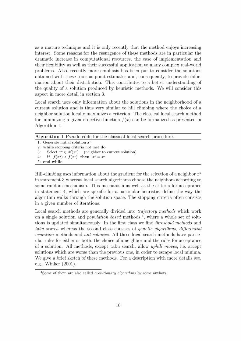
Local search uses only information about the solutions in the neighborhood of acurrent solution and is thus very similar to hill climbing where the choice of aneighbor solution locally maximizes a criterion. The classical local search methodfor minimizing a given objective function f(x) can be formalized as presented inAlgorithm 1.

Algorithm 1 Pseudo-code for the classical local search procedure.1: Generate initial solution xc

2: while stopping criteria not met do

3: Select xn ∈ N (xc) (neighbor to current solution)4: if f(xn) < f(xc) then xc = xn

5: end while

Hill-climbing uses information about the gradient for the selection of a neighbor xn

in statement 3 whereas local search algorithms choose the neighbors according tosome random mechanism. This mechanism as well as the criteria for acceptancein statement 4, which are specific for a particular heuristic, define the way thealgorithm walks through the solution space. The stopping criteria often consistsin a given number of iterations.

Local search methods are generally divided into trajectory methods which workon a single solution and population based methods,4, where a whole set of solu-tions is updated simultaneously. In the first class we find threshold methods andtabu search whereas the second class consists of genetic algorithms, differentialevolution methods and ant colonies. All these local search methods have partic-ular rules for either or both, the choice of a neighbor and the rules for acceptanceof a solution. All methods, except tabu search, allow uphill moves, i.e. acceptsolutions which are worse than the previous one, in order to escape local minima.We give a brief sketch of these methods. For a description with more details see,e.g., Winker (2001).

4Some of them are also called evolutionary algorithms by some authors.

10

2.2 Trajectory methods

The definition of neighborhood is central to these methods and generally dependson the problem under consideration. Finding efficient neighborhood functionsthat lead to high quality local optima can be challenging. For some guidelineson how to construct neighborhoods see Section 4.1. We consider three differenttrajectory methods.5 Jacobson and Yucesan (2004) present an approach for auniform treatment of these methods under the heading of generalized hill climbingalgorithms.

2.2.1 Threshold methods (TM)

The following two methods define the maximum slope for up-hill moves in thesucceeding iterations. The first method uses a probabilistic acceptance criterion,while the maximum threshold is deterministic for the second.

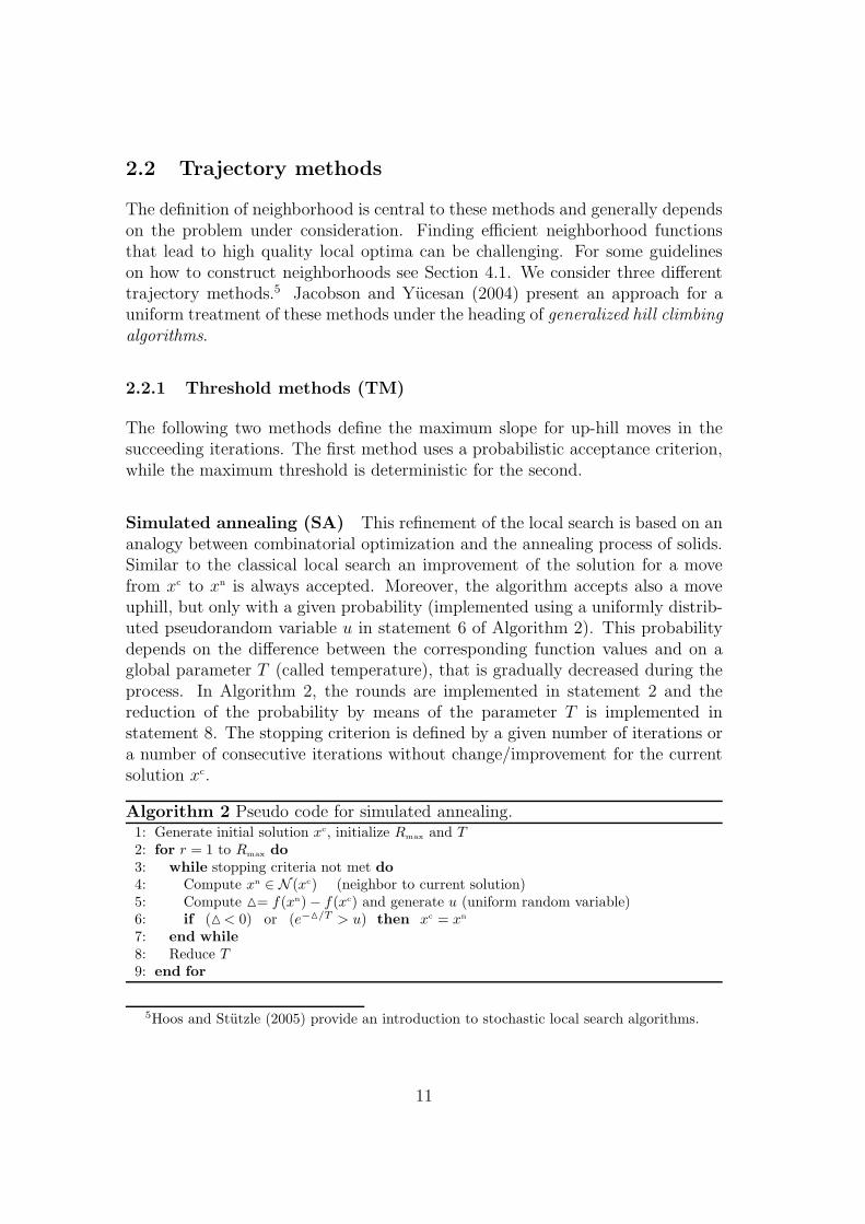
Simulated annealing (SA) This refinement of the local search is based on ananalogy between combinatorial optimization and the annealing process of solids.Similar to the classical local search an improvement of the solution for a movefrom xc to xn is always accepted. Moreover, the algorithm accepts also a moveuphill, but only with a given probability (implemented using a uniformly distrib-uted pseudorandom variable u in statement 6 of Algorithm 2). This probabilitydepends on the difference between the corresponding function values and on aglobal parameter T (called temperature), that is gradually decreased during theprocess. In Algorithm 2, the rounds are implemented in statement 2 and thereduction of the probability by means of the parameter T is implemented instatement 8. The stopping criterion is defined by a given number of iterations ora number of consecutive iterations without change/improvement for the currentsolution xc.

Algorithm 2 Pseudo code for simulated annealing.1: Generate initial solution xc, initialize Rmax and T

2: for r = 1 to Rmax do

3: while stopping criteria not met do

4: Compute xn ∈ N (xc) (neighbor to current solution)5: Compute = f(xn) − f(xc) and generate u (uniform random variable)6: if ( < 0) or (e−/T > u) then xc = xn

7: end while

8: Reduce T

9: end for

5Hoos and Stutzle (2005) provide an introduction to stochastic local search algorithms.

11

Threshold accepting (TA) This method, suggested by Dueck and Scheuer(1990), is a deterministic analog of simulated annealing where the sequence oftemperatures T is replaced by a sequence of thresholds τ . As for SA, thesethreshold values typically decrease to zero while r increases to Rmax. Algorithm 2becomes then

if < τ then xc = xn

and in statement 8 we reduce the threshold τ instead of the temperature T .6

2.2.2 Tabu search (TS)

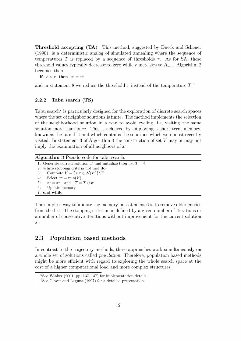
Tabu search7 is particularly designed for the exploration of discrete search spaceswhere the set of neighbor solutions is finite. The method implements the selectionof the neighborhood solution in a way to avoid cycling, i.e, visiting the samesolution more than once. This is achieved by employing a short term memory,known as the tabu list and which contains the solutions which were most recentlyvisited. In statement 3 of Algorithm 3 the construction of set V may or may notimply the examination of all neighbors of xc.

Algorithm 3 Pseudo code for tabu search.1: Generate current solution xc and initialize tabu list T = ∅2: while stopping criteria not met do

3: Compute V = x|x ∈ N (xc)\T4: Select xn = min(V )5: xc = xn and T = T ∪ xn

6: Update memory7: end while

The simplest way to update the memory in statement 6 is to remove older entriesfrom the list. The stopping criterion is defined by a given number of iterations ora number of consecutive iterations without improvement for the current solutionxc.

2.3 Population based methods

In contrast to the trajectory methods, these approaches work simultaneously ona whole set of solutions called population. Therefore, population based methodsmight be more efficient with regard to exploring the whole search space at thecost of a higher computational load and more complex structures.

6See Winker (2001, pp. 137–147) for implementation details.7See Glover and Laguna (1997) for a detailed presentation.

12

2.3.1 Genetic algorithm (GA)

These technique has been initially developed by Holland (1975).8 Genetic al-gorithms imitate the evolutionary process of species that sexually reproduce.Thus, genetic algorithms might be considered the prototype of a population basedmethod. New candidates for the solution are generated with a mechanism calledcrossover which combines part of the genetic patrimony of each parent and thenapplies a random mutation. If the new individual, called child, inherits goodcharacteristics from his parents it will have a higher probability to survive. Thefitness of the child and parent population is evaluated in function survive (state-ment 10) and the survivors can be formed either by the last generated individualsP ′′, P ′′ ∪ fittest fromP ′, only the fittest from P ′′ or the fittest from P ′ ∪ P ′′.

Algorithm 4 Pseudo code for genetic algorithms.1: Generate initial population P of solutions2: while stopping criteria not met do

3: Select P ′ ⊂ P (mating pool), initialize P ′′ = ∅ (set of children)4: for i = 1 to n do

5: Select individuals xa and xb at random from P ′

6: Apply crossover to xa and xb to produce xchild

7: Randomly mutate produced child xchild

8: P ′′ = P ′′ ∪ xchild

9: end for

10: P = survive(P ′, P ′′)11: end while

The genetic algorithm first accepts a set of solutions (statement 3) and thenconstructs a set of neighbor solutions (statements 4–10, Algorithm 4). In general,a predefined number of generation provides the stopping criterion.

2.3.2 Ant colonies (AC)

This heuristic, first introduced by Colorni et al. (1992a, 1992b) imitates the wayants search for food and find their way back to their nest. First an ant exploresits neighborhood randomly. As soon as a source of food is found it starts totransport food to the nest leaving traces of pheromone on the ground which willguide other ants to the source. The intensity of the pheromone traces dependson the quantity and quality of the food available at the source as well as from thedistance between source and nest, as for a short distance more ants will travelon the same trail in a given time interval. As the ants preferably travel alongimportant trails their behavior is able to optimize their work. Pheromone trailsevaporate and once a source of food is exhausted the trails will disappear andthe ants will start to search for other sources.

8For a more comprehensive introduction to GA see Reeves and Rowe (2003).

13

For the heuristic, the search area of the ant corresponds to a discrete set fromwhich the elements forming the solutions are selected, the amount of food isassociated with an objective function and the pheromone trail is modeled withan adaptive memory.

Algorithm 5 Pseudo code for ant colonies.1: Initialize pheromone trail2: while stopping criteria not met do

3: for all ants do

4: Deposit ant randomly5: while solution incomplete do

6: Select next element in solution randomly according to pheromone trail7: end while

8: Evaluate objective function and update best solution9: end for

10: for all ants do Update pheromone trail (more for better solutions) end for

11: end while

2.3.3 Differential evolution (DE)

Differential evolution is a population based heuristic optimization technique forcontinuous objective functions which has been introduced by Storn and Price(1997). The algorithm updates a population of solution vectors by addition,substraction and crossover and then selects the fittest solutions among the originaland updated population.

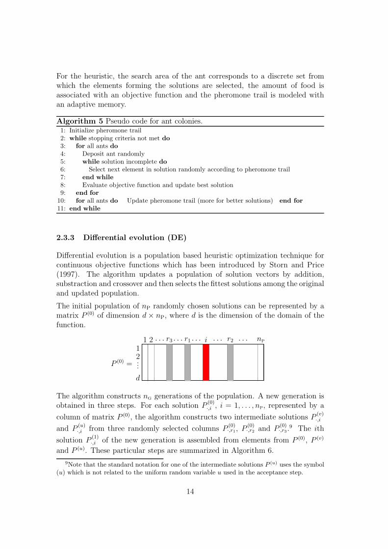
The initial population of nP randomly chosen solutions can be represented by amatrix P (0) of dimension d× nP, where d is the dimension of the domain of thefunction.

12...

d

P (0) =

1 2 · · · r3 · · · r1 · · · i · · · r2 · · · nP

The algorithm constructs nG generations of the population. A new generation isobtained in three steps. For each solution P

(0)·,i , i = 1, . . . , nP, represented by a

column of matrix P (0), the algorithm constructs two intermediate solutions P(v)·,i

and P(u)·,i from three randomly selected columns P

(0)·,r1, P

(0)·,r2 and P

(0)·,r3.

9 The ith

solution P(1)·,i of the new generation is assembled from elements from P (0), P (v)

and P (u). These particular steps are summarized in Algorithm 6.

9Note that the standard notation for one of the intermediate solutions P (u) uses the symbol(u) which is not related to the uniform random variable u used in the acceptance step.

14

Algorithm 6 Differential evolution.1: Initialize parameters nP, nG, F and CR

2: Initialize population P(1)j,i , j = 1, . . . , d, i = 1, . . . , nP

3: for k = 1 to nG do

4: P (0) = P (1)

5: for i = 1 to nP do

6: Generate r1, r2, r3 ∈ 1, . . . , nP, r1 6= r2 6= r3 6= i

7: Compute P(v)·,i = P

(0)·,r1

+ F× (P(0)·,r2

− P(0)·,r3

)8: for j = 1 to d do

9: if u < CR then P(u)j,i = P

(v)j,i else P

(u)j,i = P

(0)j,i

10: end for

11: if f(P(u)·,i ) < f(P

(0)·,i ) then P

(1)·,i = P

(u)·,i else P

(1)·,i = P

(0)·,i

12: end for

13: end for

The parameter F in statement 7 determines the length of the difference of twovectors and thus controls the speed of shrinkage in the exploration of the domain.The parameter CR together with the realization of the uniform random variableu ∼ U(0, 1) in statement 9 determines the crossover, i.e. the probability for el-

ements from P(0)·,i and P

(v)·,i to form P

(u)·,i .10 These two parameters are problem

specific. Suggested values are F = 0.8, CR = 0.8 and nP = 10 d for the popu-lation size. For these values the algorithm generally performs well for a largerange of problems. In statement 9 it is important to make sure that at least onecomponent of P

(u)·,i comes from P

(v)·,i , i.e. ∃j such that P

(u)j,i = P

(v)j,i .

2.3.4 Particle Swarm Optimization (PS)

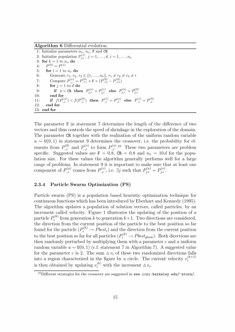
Particle swarm (PS) is a population based heuristic optimization technique forcontinuous functions which has been introduced by Eberhart and Kennedy (1995).The algorithm updates a population of solution vectors, called particles, by anincrement called velocity. Figure 1 illustrates the updating of the position of aparticle P

(k)i from generation k to generation k+1. Two directions are considered,

the direction from the current position of the particle to the best position so farfound for the particle (P

(k)i → Pbest i) and the direction from the current position

to the best position so far for all particles (P(k)i → Pbestgbest). Both directions are

then randomly perturbed by multiplying them with a parameter c and a uniformrandom variable u ∼ U(0, 1) (c.f. statement 7 in Algorithm 7). A suggested valuefor the parameter c is 2. The sum vi of these two randomized directions fallsinto a region characterized in the figure by a circle. The current velocity v

(k+1)i

is then obtained by updating v(k)i with the increment vi.

10Different strategies for the crossover are suggested in www.icsi.berkeley.edu/∼storn/.

15

P(k)i

v(k)i

Pbest i

Pbestgbest

vi

P(k+1)i

v(k+1)i

Figure 1: Updating the position of a particle P(k)i with velocity v

(k)i .

Algorithm 7 summarizes the particular steps for the updating of the populationof nP particles in nG succeeding generations.

Algorithm 7 Particle swarm.1: Initialize parameters nP, nG and c

2: Initialize particles P(0)i and velocity v

(0)i , i = 1, . . . , nP

3: Evaluate objective function Fi = f(P(0)i ), i = 1, . . . , nP

4: Pbest = P (0), Fbest = F , Gbest = mini(Fi), gbest = argmini(Fi)5: for k = 1 to nG do

6: for i = 1 to nP do

7: vi = c u (Pbest i − P(k−1)i ) + c u (Pbestgbest − P

(k−1)i )

8: v(k)i = v(k−1)+ vi

9: P(k)i = P

(k−1)i + v

(k)i

10: end for

11: Evaluate objective function Fi = f(P(k)i ), i = 1, . . . , nP

12: for i = 1 to nP do

13: if Fi < Fbest i then Pbest i = P(k)i and Fbest i = Fi

14: if Fi < Gbest then Gbest = Fi and gbest = i

15: end for

16: end for

2.4 Hybrid meta-heuristics

In a general framework optimization heuristics are also called meta-heuristics11

which can be considered as a general skeleton of an algorithm applicable to awide range of problems. A meta-heuristic may evolve to a particular heuristicwhen it is specialized to solve a particular problem. Meta-heuristics are madeup by different components and if components from different meta-heuristicsare assembled we obtain a hybrid meta-heuristic. This allows us to imagine alarge number of new techniques. The construction of hybrid meta-heuristics is

11Apart this section, we do not follow this convention, but use the term heuristic synony-mously.

16

motivated by the need to achieve a good tradeoff between the capabilities of aheuristic to explore the search space and the possibility to exploit the experienceaccumulated during the search.12

In order to get a more compact view of the possibilities and types of hybrid meta-heuristics one can imagine, we will present a short and informal classification ofthe different meta-heuristics, describe the basic characteristics of the differentcomponents and give examples of hybrid approaches.13

2.4.1 Basic characteristics of meta-heuristics

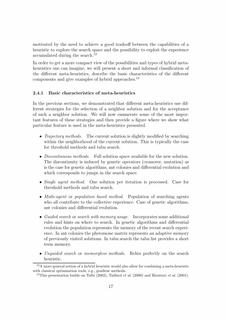
In the previous sections, we demonstrated that different meta-heuristics use dif-ferent strategies for the selection of a neighbor solution and for the acceptanceof such a neighbor solution. We will now enumerate some of the most impor-tant features of these strategies and then provide a figure where we show whatparticular feature is used in the meta-heuristics presented.

• Trajectory methods. The current solution is slightly modified by searchingwithin the neighborhood of the current solution. This is typically the casefor threshold methods and tabu search.

• Discontinuous methods. Full solution space available for the new solution.The discontinuity is induced by genetic operators (crossover, mutation) asis the case for genetic algorithms, ant colonies and differential evolution andwhich corresponds to jumps in the search space.

• Single agent method. One solution per iteration is processed. Case forthreshold methods and tabu search.

• Multi-agent or population based method. Population of searching agentswho all contribute to the collective experience. Case of genetic algorithms,ant colonies and differential evolution.

• Guided search or search with memory usage. Incorporates some additionalrules and hints on where to search. In genetic algorithms and differentialevolution the population represents the memory of the recent search experi-ence. In ant colonies the pheromone matrix represents an adaptive memoryof previously visited solutions. In tabu search the tabu list provides a shortterm memory.

• Unguided search or memoryless methods. Relies perfectly on the searchheuristic.

12A more general notion of a hybrid heuristic would also allow for combining a meta-heuristicwith classical optimization tools, e.g., gradient methods.

13This presentation builds on Talbi (2002), Taillard et al. (2000) and Birattari et al. (2001).

17

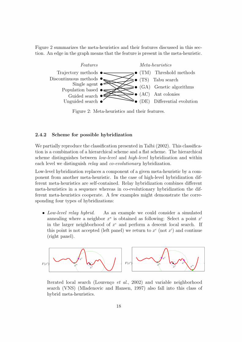
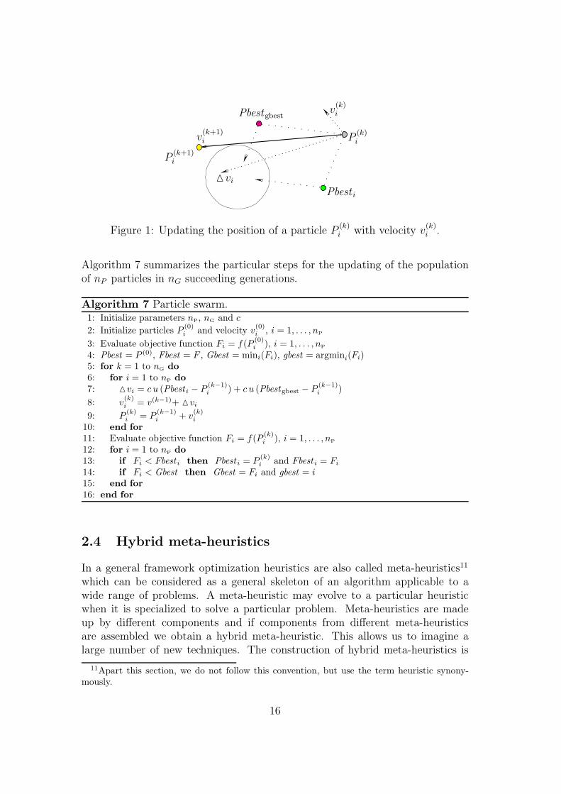
Figure 2 summarizes the meta-heuristics and their features discussed in this sec-tion. An edge in the graph means that the feature is present in the meta-heuristic.

Features Meta-heuristics

Trajectory methods

Discontinuous methodsSingle agent

Population based

Guided searchUnguided search

(TM) Threshold methods

(TS) Tabu search

(GA) Genetic algorithms

(AC) Ant colonies

(DE) Differential evolution

Figure 2: Meta-heuristics and their features.

2.4.2 Scheme for possible hybridization

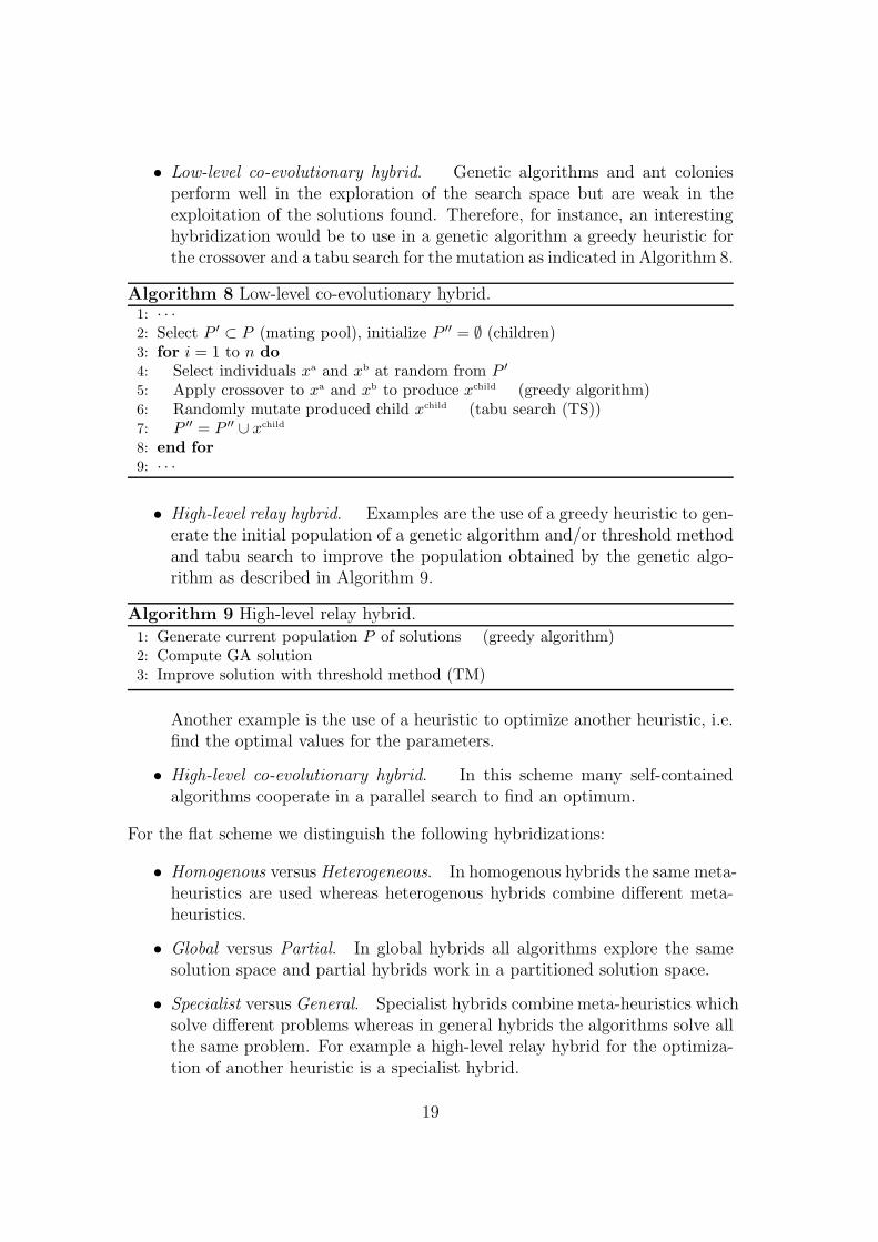
We partially reproduce the classification presented in Talbi (2002). This classifica-tion is a combination of a hierarchical scheme and a flat scheme. The hierarchicalscheme distinguishes between low-level and high-level hybridization and withineach level we distinguish relay and co-evolutionary hybridization.

Low-level hybridization replaces a component of a given meta-heuristic by a com-ponent from another meta-heuristic. In the case of high-level hybridization dif-ferent meta-heuristics are self-contained. Relay hybridization combines differentmeta-heuristics in a sequence whereas in co-evolutionary hybridization the dif-ferent meta-heuristics cooperate. A few examples might demonstrate the corre-sponding four types of hybridizations:

• Low-level relay hybrid. As an example we could consider a simulatedannealing where a neighbor xn is obtained as following: Select a point xi

in the larger neighborhood of xc and perform a descent local search. Ifthis point is not accepted (left panel) we return to xc (not xi) and continue(right panel).

xc

F (xc)

xi

xn

xc

F (xc)

xi

xn xi

xn

Iterated local search (Lourenco et al., 2002) and variable neighborhoodsearch (VNS) (Mladenovic and Hansen, 1997) also fall into this class ofhybrid meta-heuristics.

18

• Low-level co-evolutionary hybrid. Genetic algorithms and ant coloniesperform well in the exploration of the search space but are weak in theexploitation of the solutions found. Therefore, for instance, an interestinghybridization would be to use in a genetic algorithm a greedy heuristic forthe crossover and a tabu search for the mutation as indicated in Algorithm 8.

Algorithm 8 Low-level co-evolutionary hybrid.1: · · ·2: Select P ′ ⊂ P (mating pool), initialize P ′′ = ∅ (children)3: for i = 1 to n do

4: Select individuals xa and xb at random from P ′

5: Apply crossover to xa and xb to produce xchild (greedy algorithm)6: Randomly mutate produced child xchild (tabu search (TS))7: P ′′ = P ′′ ∪ xchild

8: end for

9: · · ·

• High-level relay hybrid. Examples are the use of a greedy heuristic to gen-erate the initial population of a genetic algorithm and/or threshold methodand tabu search to improve the population obtained by the genetic algo-rithm as described in Algorithm 9.

Algorithm 9 High-level relay hybrid.

1: Generate current population P of solutions (greedy algorithm)2: Compute GA solution3: Improve solution with threshold method (TM)

Another example is the use of a heuristic to optimize another heuristic, i.e.find the optimal values for the parameters.

• High-level co-evolutionary hybrid. In this scheme many self-containedalgorithms cooperate in a parallel search to find an optimum.

For the flat scheme we distinguish the following hybridizations:

• Homogenous versus Heterogeneous. In homogenous hybrids the same meta-heuristics are used whereas heterogenous hybrids combine different meta-heuristics.

• Global versus Partial. In global hybrids all algorithms explore the samesolution space and partial hybrids work in a partitioned solution space.

• Specialist versus General. Specialist hybrids combine meta-heuristics whichsolve different problems whereas in general hybrids the algorithms solve allthe same problem. For example a high-level relay hybrid for the optimiza-tion of another heuristic is a specialist hybrid.

19

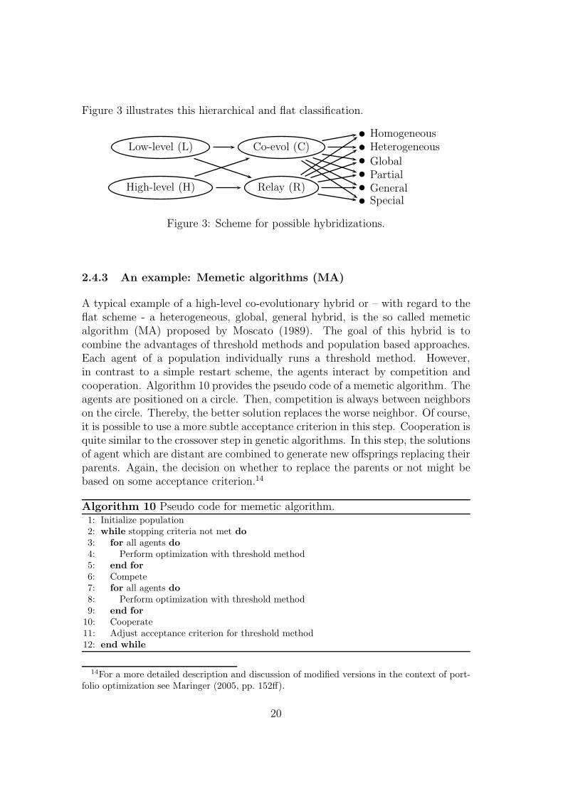
Figure 3 illustrates this hierarchical and flat classification.

HomogeneousHeterogeneous

GlobalPartialGeneralSpecial

Co-evol (C)

Relay (R)

Low-level (L)

High-level (H)

Figure 3: Scheme for possible hybridizations.

2.4.3 An example: Memetic algorithms (MA)

A typical example of a high-level co-evolutionary hybrid or – with regard to theflat scheme - a heterogeneous, global, general hybrid, is the so called memeticalgorithm (MA) proposed by Moscato (1989). The goal of this hybrid is tocombine the advantages of threshold methods and population based approaches.Each agent of a population individually runs a threshold method. However,in contrast to a simple restart scheme, the agents interact by competition andcooperation. Algorithm 10 provides the pseudo code of a memetic algorithm. Theagents are positioned on a circle. Then, competition is always between neighborson the circle. Thereby, the better solution replaces the worse neighbor. Of course,it is possible to use a more subtle acceptance criterion in this step. Cooperation isquite similar to the crossover step in genetic algorithms. In this step, the solutionsof agent which are distant are combined to generate new offsprings replacing theirparents. Again, the decision on whether to replace the parents or not might bebased on some acceptance criterion.14

Algorithm 10 Pseudo code for memetic algorithm.1: Initialize population2: while stopping criteria not met do

3: for all agents do

4: Perform optimization with threshold method5: end for

6: Compete7: for all agents do

8: Perform optimization with threshold method9: end for

10: Cooperate11: Adjust acceptance criterion for threshold method12: end while

14For a more detailed description and discussion of modified versions in the context of port-folio optimization see Maringer (2005, pp. 152ff).

20

3 Stochastics of the solution

Given the dominating classical optimization paradigm, it is not too surprisingthat the analysis of the results obtained by optimization heuristics concentrateson the probability to obtain the global optimum. In fact, some optimization al-gorithms allow to derive quite general convergence results as will be describedin Subsection 3.2. However, for practical implementations, it might be more in-teresting to know the relationship between computational resources spent andthe quality of the solution obtained.15 Furthermore, often it is less the conver-gence of the objective function one is interested in, but, e.g., the convergenceof the parameters estimated by optimizing the objective function. This aspectwill be discussed in Subsection 3.3. Before turning to convergence issues, westart by providing a formal framework for the analysis of the results obtained byoptimization heuristics.

3.1 Optimization as stochastic mapping

Whenever repeated applications of an optimization method do not generate iden-tical results, we have to deal with this type of stochastics, which is different fromthe stochastics resulting from random sampling. For the optimization heuristicsintroduced in the previous section, the generation of an initial solution (popula-tion), the selection of candidate solutions in each search step and sometimes alsothe acceptance decision are responsible for this type of randomness. It shouldbe noted that the use of classical methods might also generate additional ran-domness, e.g., when using randomly generated starting values. In both cases, i.e.independent from the classification as classical or heuristic method, the outcomeof a single run of the optimization procedure has to be interpreted as a randomdrawing from some a priori unknown distribution.

From the point of view of an applied econometrician, this additional randomnessmight be considered as a rather unwelcome feature of optimization heuristicsas compared to standard optimization tools. However, a classical tool mightwell provide a deterministic solution which might be far away from the optimalsolution if it is applied to a problem which does not meet the requirements forthe method to converge to the global optimum. In such a situation, it is evidentthat a stochastic approximation to the true optimum might be preferable to abad deterministic result. Furthermore, econometricians are well trained in dealingwith the stochastics resulting from random sampling. Therefore, it seems sensiblealso to consider the stochastics of the outcome of optimization heuristics in somemore detail.

Let ψψψI,r denote the result of a run r = 1, . . . , nRestarts of an optimization heuristic

15For an example, see Brooks and Morgan (1995, p. 243).

21

H for a given problem instance with objective function f . Thereby, I denotesa measure of the computational resources spent for a single run, e.g., numberof local search steps for a local search heuristic or number of generations for agenetic algorithm. The value of the objective function obtained in run r amountsto f(ψψψI,r). This value can be interpreted as a random drawing from a distri-bution DH

I (µI , σI , . . .). It is assumed that the expectation and variance of thisdistribution exist and are finite.

Although, for most optimization heuristics H , specific knowledge about the dis-tribution DH

I (µI , σI , . . .) is very limited for most applications,16 some generalproperties of the distribution can be derived. First, for minimization problems,the distribution will be left censored at the global minimum of f denoted by fmin

in the following. Second, with increasing amount of computational resources I,the distribution should shift left and become less dispersed, i.e. µI′ ≤ µI andσI′ ≤ σI for all I ′ > I. Finally, for those applications, where asymptotical con-vergence in probability can be proven, the distribution becomes degenerate as Itends to infinity. It is beyond the scope of this contribution to develop a the-ory for DH

I . Some ideas on how to build such a theory for the case of localsearch heuristics like simulated annealing and threshold accepting can be foundin the convergence results presented by Aarts and Korst (1989) and Althofer andKoschnik (1991).17 A modelling approach for finite I is presented by Jacobsonet al. (2006).

Applying an optimization heuristic repeatedly to the same problem instancemakes it possible to calculate the empirical distribution function of f(ψψψI,r),r = 1, . . . , nRestarts. This distribution function can be used to assess propertiesof DH

I and to estimate its empirical moments. In particular, lower quantiles willbe of highest interest as estimates of the best solutions which might be expectedin an application to a minimization problem. Furthermore, extreme value theorymight be used to obtain estimates of the unknown global minimum (Husler etal., 2003). Finally, repeating the exercise for different amounts of computationalresources I might allow estimation of an empirical rate of convergence.

Figure 4 presents results from an application of the threshold accepting heuristicto the problem of lag structure selection in VAR models.18 Some details of thethreshold accepting implementation are presented in Section 5.1 below. The up-per left plot exhibits the empirical distribution functions of the objective function(Bayesian information criterion) for different values of I (from right to left forI = 100, 500, 1000, 5000, 10000). As theoretically expected, the distributionsmove left (µI is decreasing) and become steeper (σI is decreasing) with I grow-

16Pure random sampling might be an exception for problems with well-defined and easy tomodel search space.

17See also Rudolph (1997) and Reeves and Rowe (2003).18For a discussion of VAR models – model selection and estimation – see Lutkepohl (2007)

in this volume.

22

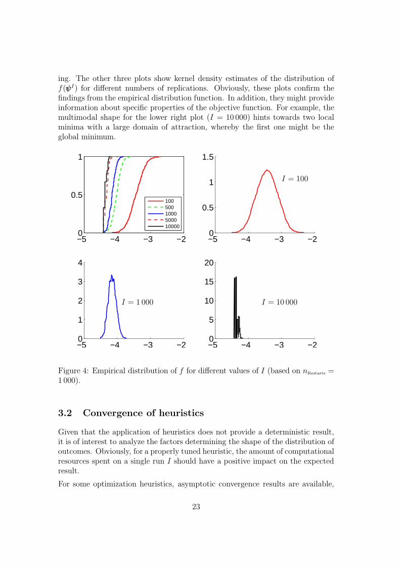
ing. The other three plots show kernel density estimates of the distribution off(ψψψI) for different numbers of replications. Obviously, these plots confirm thefindings from the empirical distribution function. In addition, they might provideinformation about specific properties of the objective function. For example, themultimodal shape for the lower right plot (I = 10 000) hints towards two localminima with a large domain of attraction, whereby the first one might be theglobal minimum.

−5 −4 −3 −20

0.5

1

1005001000500010000

−5 −4 −3 −20

0.5

1

1.5

−5 −4 −3 −20

1

2

3

4

−5 −4 −3 −20

5

10

15

20

I = 100

I = 1 000 I = 10 000

Figure 4: Empirical distribution of f for different values of I (based on nRestarts =1 000).

3.2 Convergence of heuristics

Given that the application of heuristics does not provide a deterministic result,it is of interest to analyze the factors determining the shape of the distribution ofoutcomes. Obviously, for a properly tuned heuristic, the amount of computationalresources spent on a single run I should have a positive impact on the expectedresult.

For some optimization heuristics, asymptotic convergence results are available,

23

e.g., simulated annealing (Aarts and Korst, 1989), threshold accepting (Althoferand Koschnik, 1991), and genetic algorithm (Reeves and Rowe, 2003, pp. 111ff).These results can be interpreted in the formal framework introduced in the pre-vious subsection. Although the results indicate that µI and σI decrease as Itends to infinity, they do not provide quantitative information, e.g., on the rateof convergence. Hence, further research is required regarding these convergenceproperties.

In the following, we will present the results for threshold accepting obtained byAlthofer and Koschnik (1991) as an example. Similar reasoning might apply forother convergent heuristics. The empirical assessment also focuses on thresholdaccepting, but, again, the approach might be used for other heuristics as well.

First, it has to be noted that the results depend on a number of assumptionsregarding the problem instance. In particular, the objective function has tosatisfy certain conditions, and the search space has to be connected, i.e. it shouldbe possible to reach any point of the search space from any given starting point byperforming local search steps. Second, the results are existence results. Althoferand Koschnik (1991) prove that there exist suitable parameters for the thresholdaccepting implementation such that the global optimum of the objective functioncan be approximated at arbitrary accuracy with any fixed probability close toone by increasing the number of iterations. Unfortunately, finding the suitableparameter values is a different task.

Under the assumptions just mentioned and formalized in Althofer and Koschnik(1991), the following convergence result is obtained: For any given δ > 0 andε > 0, there exists a number of iterations I(δ, ε) such that for any replicationr = 1, . . . , nRestarts

P(|f(ψψψI,r) − fmin| < ε) > 1 − δ , (1)

where fmin denotes the global minimum of the objective function. When con-sidering only the best out of nRestarts replications, a smaller number of iterationsmight be sufficient for given values of δ and ε.

Although such a global convergence result might be considered a prerequisitefor considering an optimization heuristic in an econometric context, it is not asufficient property. In fact, at least two points deserve further attention. First,given that it is not realistic to spend an unlimited amount of computationalresources, it is of interest to know at which rate µI converges to fmin and σI

converges to zero as I tends to infinity. So far, we are not aware of any theoreticalresults on this issue, but we will discuss some empirical results in the following.Second, as long as σI is not zero, i.e. typically for any finite value of I, anydeviation in fitting the global minimum of the objective function is linked to anerror in the approximation of a specific estimator. The following subsection willprovide some arguments on this issue.

24

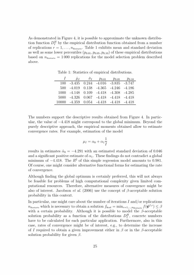
As demonstrated in Figure 4, it is possible to approximate the unknown distribu-tion function DH

I by the empirical distribution function obtained from a numberof replications r = 1, . . . , nRestarts. Table 1 exhibits mean and standard deviationas well as some lower percentiles (p0.01, p0.05, p0.10) of these empirical distributionsbased on nRestarts = 1 000 replications for the model selection problem describedabove.

Table 1: Statistics of empirical distributions.

I µI σI p0.01 p0.05 p0.10

100 -3.435 0.244 -4.016 -3.835 -3.747500 -4.019 0.138 -4.365 -4.246 -4.186

1000 -4.148 0.109 -4.418 -4.308 -4.2855000 -4.326 0.067 -4.418 -4.418 -4.418

10000 -4.359 0.054 -4.418 -4.418 -4.418

The numbers support the descriptive results obtained from Figure 4. In partic-ular, the value of −4.418 might correspond to the global minimum. Beyond thepurely descriptive approach, the empirical moments obtained allow to estimateconvergence rates. For example, estimation of the model

µI = α0 + α11

I

results in estimates α0 = −4.291 with an estimated standard deviation of 0.046and a significant positive estimate of α1. These findings do not contradict a globalminimum of −4.418. The R2 of this simple regression model amounts to 0.981.Of course, one might consider alternative functional forms for estimating the rateof convergence.

Although finding the global optimum is certainly preferred, this will not alwaysbe feasible for problems of high computational complexity given limited com-putational resources. Therefore, alternative measures of convergence might bealso of interest. Jacobson et al. (2006) use the concept of β-acceptable solutionprobability in this context.

In particular, one might care about the number of iterations I and/or replicationsnRestarts which is necessary to obtain a solution fbest = minr=1,...,nRestarts

f(ψψψI,r) ≤ βwith a certain probability. Although it is possible to model the β-acceptablesolution probability as a function of the distributions DH

I , concrete numbershave to be calculated for each particular application. Furthermore, also in thiscase, rates of convergence might be of interest, e.g., to determine the increaseof I required to obtain a given improvement either in β or in the β-acceptablesolution probability for given β.

25

Typically, an optimization heuristic is applied repeatedly to the same probleminstance. Therefore, the result reported will correspond to the best out of nRestarts

replications, also called restarts. Obviously, the expected value for this bestresult will be better than for a single run. Extreme value analysis might be usedto derive results on the distribution in this situation. Then, the results of theanalysis might be used to derive an optimal number of restarts. For some ideason this issue from the application point of view see the paragraph on restarts inSection 4.1 below.

Given that optimization heuristics start playing a more important role in econo-metrics, we argue that further research on these and similar aspects of theirapplication is highly relevant and urgently needed.

3.3 Convergence of optimization based estimators

When optimization heuristics are applied to estimation problems like, e.g., cen-sored quantile regression or (augmented) GARCH models, the stochastics of theoptimization algorithm interferes with the stochastics of the estimators. Weprovide a formal description of this inference and demonstrate that, at least as-ymptotically, this interference favors the application of optimization heuristics.In fact, it is possible to derive joint convergence results.

Let us assume that the sample size T grows to infinity and that the theoreticalestimator ψψψT will converge to its “true” value ψψψ in probability. We consider theimplementation of a convergent heuristic, i.e. we might assume that the heuristicconverges in probability to the global optimum corresponding to ψψψT with I goingto infinity. Furthermore, we assume that the search space for ψψψT is a compactset and that the estimation function is continuous.19 Then, given δ > 0 andε > 0 it is possible to choose the number of iterations I as a function of T, δ, andε such that the estimate obtained using the heuristic ψψψI

T satisfies the followinginequality:

P(|ψψψIT − ψψψT | < ε) > 1 − δ . (2)

Combining this result with the convergence in probability of the estimator, oneobtains a joint convergence result: There exists a function I(T ) for the number

of iterations such that the estimate ψψψI(T )T converges in probability to the true

parameter vectorψψψ. Although this result is not precise with regard to the choice ofI(T ), it bears some promises in cases where classical methods might not converge

to ψψψT . For a more detailed description see Fitzenberger and Winker (2007) andMaringer and Winker (2006).

As for the objective function itself, the convergence of parameter estimates might

19In passing note that these conditions are sufficient for the following results to hold but notnecessary. One can probably obtain the results under much weaker assumptions.

26

be improved when considering the best result (with regard to f) out of a numberof nRestarts restarts of the optimization heuristic. The analysis of this effect bymeans of extreme value theory is a topic of current research.

4 General guidelines for the use of optimization

heuristics

The first questions to be answered for a specific application is whether to use anoptimization heuristic at all and if so, which one to employ. Unfortunately, bothquestions do not allow for a general answer. Obviously, when a problem is knownto be computational complex, e.g., due to several local minima, we recommendto apply an optimization heuristic as a benchmark for classical optimization pro-cedures. Whenever the application of the heuristic generates better results atleast for some replications, this is a clear indication for the use of such methods.Then, a more careful implementation analysis should follow. In fact, given agrowing availability of code for some optimization heuristics on different softwareplatforms, their use as a benchmark might become more standard.

The second choice is with regard to the heuristic itself. One selection can bebased on the properties of the search space and the objective function givenas some heuristics like DE are not well suited to tackle discrete optimizationproblems or problems with noise in the objective function. Another motivationfor a specific optimization heuristic consists in previous (own) experience witha method for problems exhibiting similar characteristics. Finally, we argue thatone should start with a simple general heuristic before turning to more problemspecific hybrids.

Irrespective of the specific method chosen, any implementation of the algorithmspresented in Section 2 needs particular attention with respect to a number ofdetails, a task which is generally left to the user. For instance in the case ofa trajectory method the neighborhood solution should be easy to generate, thedefinition of the neighborhood should not be too large and the topology of theobjective function not too flat. Population based methods or evolutionary algo-rithms perform in each iteration a mechanism of co-operation and a mechanism ofself-adaption. In a genetic algorithm information is exchanged among individu-als during crossover which can be considered as co-operation, while mutation is aself-adaptation process. It is then important that pertinent information is trans-mitted during co-operation. The combination of two equivalent parent solutionsshould not produce an offspring that is different from the parents. The preserva-tion of the diversity in the population is also very important for the efficiency ofthe algorithm.

Rather than covering the details of a large variety of methods this section aims

27

at providing some basic principles for the successful adaptation of heuristics indifficult optimization problems. We present these principles for the thresholdaccepting algorithm with its particularly simple structure.

We consider a minimization problem on a subset Ω of Rk:

minx∈Ω

f(x) Ω ⊂ Rk . (3)

For applications to discrete optimization problems see, e.g., Section 5.1.

4.1 Implementation

The implementation of the threshold accepting algorithm involves the definitionof the objective function, the neighborhood and the threshold sequence. Moreoverone has to specify the number of restarts nRestarts,

20 the number of rounds nRounds

in which the threshold is reduced to zero and the number of steps nSteps thealgorithm searches neighbor solutions for a given value τr of the threshold. Then,the number of iterations per restart is given by I = nRounds × nSteps.

Objective function and constraints

Local search essentially proceeds in successive evaluations and comparisons ofthe objective function and therefore the performance of the heuristic cruciallydepends on its fast calculation. To improve this performance, the objectivefunction should, whenever possible, be locally updated, i.e. the difference ∆ =f(xn) − f(xc) between the value of the objective function for a current solutionxc and a neighbor solution xn should be computed directly by updating f(xc)and not by computing f(xn) from scratch. If possible, local updating will alsoimprove the performance of population based algorithms. However, local updat-ing requires a detailed analysis of the objective function. In the fields of statisticsand econometrics, we are only aware of the applications to experimental designby Fang et al. (2003) and Fang et al. (2005) making use of local updating.

We use the classical traveling salesman problem from operations research to de-scribe the idea of local updating. The problem consists in finding a tour ofminimum length going through a given number of cities. Starting with somerandom tour, a local modification is given by exchange the sequence of two citiesin the tour. Obviously, the length of the new tour has not to be calculated fromscratch, but can be obtained from the length of the previous tour by subtractingthe length of the removed links and adding the length of the new links. Thespeed up will be considerable as soon as the number of cities becomes large.

20Algorithm 12 below provides the pseudo code for the implementation with restarts.

28

In the presence of constraints the search space Ω is a subspace Ω ⊂ Rk. The

generation of starting and neighbor solutions which are elements of Ω mightbe difficult, in particular if Ω is not connected. Therefore, R

k should be used assearch space and a penalty term added to the objective function if x 6∈ Ω. In orderto allow the exploration of the whole search space, the penalty term is usually setat small values at the beginning of an optimization run. It is increased with thenumber of rounds to rather high values at the end of the run to guarantee thatthe final solution is a feasible one. If expressed in absolute terms, these scheme ofpenalty terms has to be adjusted for every application. Alternatively, one mightuse relative penalty terms allowing for more general implementations.

The handling of constraints is also an issue in population based algorithms unlessall operators can be constructed in a way to guarantee that only feasible solutionscan result.

Neighborhood definition

The objective function should exhibit local behavior with regard to the closerneighborhood, denoted N (x), of a solution x. This means that for elementsxn ∈ N (x), the objective function should be closer to f(x) than for randomlyselected points xr. Of course, there is a trade-off between large neighborhoods,which guarantee non-trivial projections and small neighborhoods with a real localbehavior of the objective function.

For real valued variables, a straightforward definition of the neighborhood is givenby means of ε-spheres

N (xc) = xn|xn ∈ Rk and ‖xn − xc‖ < ε ,

where ‖ · ‖ denotes the Euclidian metric. In the case of a discrete search space,one might use the Hamming metric instead (Hamming, 1950). A drawback ofthis definition in the Euclidian case is that the generation of elements in N (xc)might be computational costly. A simpler method consists in considering hyper-rectangles, possibly only in a few randomly selected dimensions, i.e. to selectrandomly a subset of elements xc

i , i ∈ J ⊂ 1, 2, . . . , k for which ‖xni − xc

i‖ < ε.For many applications a choice with #J = 1, i.e. where we modify a singleelement of xc, works very well.

Threshold sequence

The theoretical analysis of the threshold accepting algorithm in Althofer andKoschnik (1991) does not provide a guideline on how to choose the thresholdsequence. In fact, for a very small problem, Althofer and Koschnik (1991, p. 194)even show that the optimal threshold sequence is not monotonically decreasing.

29

Nevertheless, for applications in econometrics, two simple procedures seem toprovide useful threshold sequences. First, one might use a linear schedule de-creasing to zero over the number of rounds. Obviously, for this sequence, onlythe first threshold value is subject to some parameter tuning. Second, one mightexploit the local structure of the objective function for a data driven generationof the threshold sequence.

A motivation for this second approach can be provided for a finite search space.In this case, only threshold values corresponding to the difference of the objec-tive function values for a pair of neighbours are relevant. Given the number ofelements in real search spaces, it is not possible to calculate all these values. In-stead, one uses a random sample from the distribution of such local differences.This procedure can also be applied to the cases of infinite and continuous searchspaces.

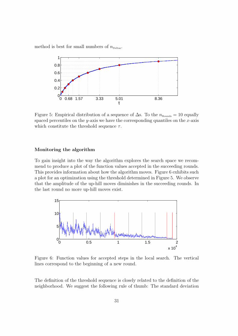
Algorithm 11 provides the details of the procedure. On starts with a randomlyselected point xc ∈ Ω, chooses a randomly selected neighbour xn ∈ N (xc) andcalculates the absolute value of the difference in the objective function ∆ =|f(xc) − f(xn)|. Next, xc is replaced by xn and the steps are repeated a certainnumber of times nDeltas ≥ nRounds. The resulting empirical distribution of ∆s isshown in Figure 5. For very large values of the threshold, the search procedureresembles closely a pure random search. Thus, it is often useful to consider only alower quantile of the empirical distribution function. Then, based on the nRounds

smallest ∆s, the threshold sequence can be computed as proposed by Winkerand Fang (1997) and used in several applications afterwards. It is given by thequantiles corresponding to a vector of equidistant percentiles Pi = (nRounds −i)/nRounds, i = 1, . . . , nRounds. Figure 5 also provides the threshold sequence τ fornRounds = 10 for the application presented in Section 5.2 below.

Algorithm 11 Generation of threshold sequence.1: Randomly choose xc ∈ Ω2: for i = 1 to nDeltas do

3: Compute xn ∈ N (xc) and ∆i = |f(xc) − f(xn)|4: xc = xn

5: end for

6: Compute empirical distribution F of ∆i, i = 1, . . . , nSteps

7: Compute threshold sequence τr = F−1(

nRounds−r

nRounds

)

, r = 1, . . . , nRounds

Instead of considering the local changes of the objective function ∆ along a paththrough the search space as described in Algorithm 11, one might consider severalrestarts to produce different trajectories of shorter length, or – in the limit –generate all xc randomly. Obviously, when letting nDeltas tend to infinity, allthree methods should provide the same approximation to the distribution of localchanges of the objective function. However, we do not have clear evidence which

30

method is best for small numbers of nDeltas.

0 0.68 1.57 3.33 5.01 8.360

0.2

0.4

0.6

0.8

1

τ

Figure 5: Empirical distribution of a sequence of ∆s. To the nRounds = 10 equallyspaced percentiles on the y-axis we have the corresponding quantiles on the x-axiswhich constitute the threshold sequence τ .

Monitoring the algorithm

To gain insight into the way the algorithm explores the search space we recom-mend to produce a plot of the function values accepted in the succeeding rounds.This provides information about how the algorithm moves. Figure 6 exhibits sucha plot for an optimization using the threshold determined in Figure 5. We observethat the amplitude of the up-hill moves diminishes in the succeeding rounds. Inthe last round no more up-hill moves exist.

0 0.5 1 1.5 2

x 104

0

5

10

15

Figure 6: Function values for accepted steps in the local search. The verticallines correspond to the beginning of a new round.

The definition of the threshold sequence is closely related to the definition of theneighborhood. We suggest the following rule of thumb: The standard deviation

31

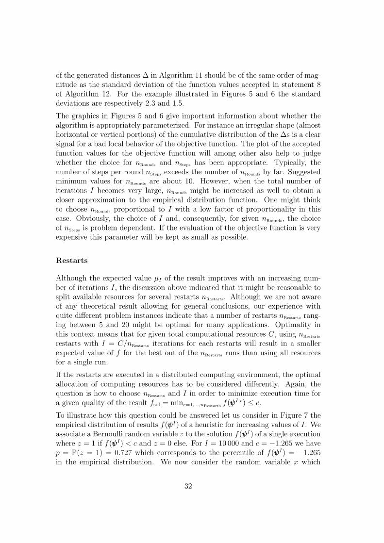
of the generated distances ∆ in Algorithm 11 should be of the same order of mag-nitude as the standard deviation of the function values accepted in statement 8of Algorithm 12. For the example illustrated in Figures 5 and 6 the standarddeviations are respectively 2.3 and 1.5.

The graphics in Figures 5 and 6 give important information about whether thealgorithm is appropriately parameterized. For instance an irregular shape (almosthorizontal or vertical portions) of the cumulative distribution of the ∆s is a clearsignal for a bad local behavior of the objective function. The plot of the acceptedfunction values for the objective function will among other also help to judgewhether the choice for nRounds and nSteps has been appropriate. Typically, thenumber of steps per round nSteps exceeds the number of nRounds by far. Suggestedminimum values for nRounds are about 10. However, when the total number ofiterations I becomes very large, nRounds might be increased as well to obtain acloser approximation to the empirical distribution function. One might thinkto choose nRounds proportional to I with a low factor of proportionality in thiscase. Obviously, the choice of I and, consequently, for given nRounds, the choiceof nSteps is problem dependent. If the evaluation of the objective function is veryexpensive this parameter will be kept as small as possible.

Restarts

Although the expected value µI of the result improves with an increasing num-ber of iterations I, the discussion above indicated that it might be reasonable tosplit available resources for several restarts nRestarts. Although we are not awareof any theoretical result allowing for general conclusions, our experience withquite different problem instances indicate that a number of restarts nRestarts rang-ing between 5 and 20 might be optimal for many applications. Optimality inthis context means that for given total computational resources C, using nRestarts

restarts with I = C/nRestarts iterations for each restarts will result in a smallerexpected value of f for the best out of the nRestarts runs than using all resourcesfor a single run.

If the restarts are executed in a distributed computing environment, the optimalallocation of computing resources has to be considered differently. Again, thequestion is how to choose nRestarts and I in order to minimize execution time fora given quality of the result fsol = minr=1,...,nRestarts

f(ψψψI,r) ≤ c.

To illustrate how this question could be answered let us consider in Figure 7 theempirical distribution of results f(ψψψI) of a heuristic for increasing values of I. Weassociate a Bernoulli random variable z to the solution f(ψψψI) of a single executionwhere z = 1 if f(ψψψI) < c and z = 0 else. For I = 10 000 and c = −1.265 we havep = P(z = 1) = 0.727 which corresponds to the percentile of f(ψψψI) = −1.265in the empirical distribution. We now consider the random variable x which

32

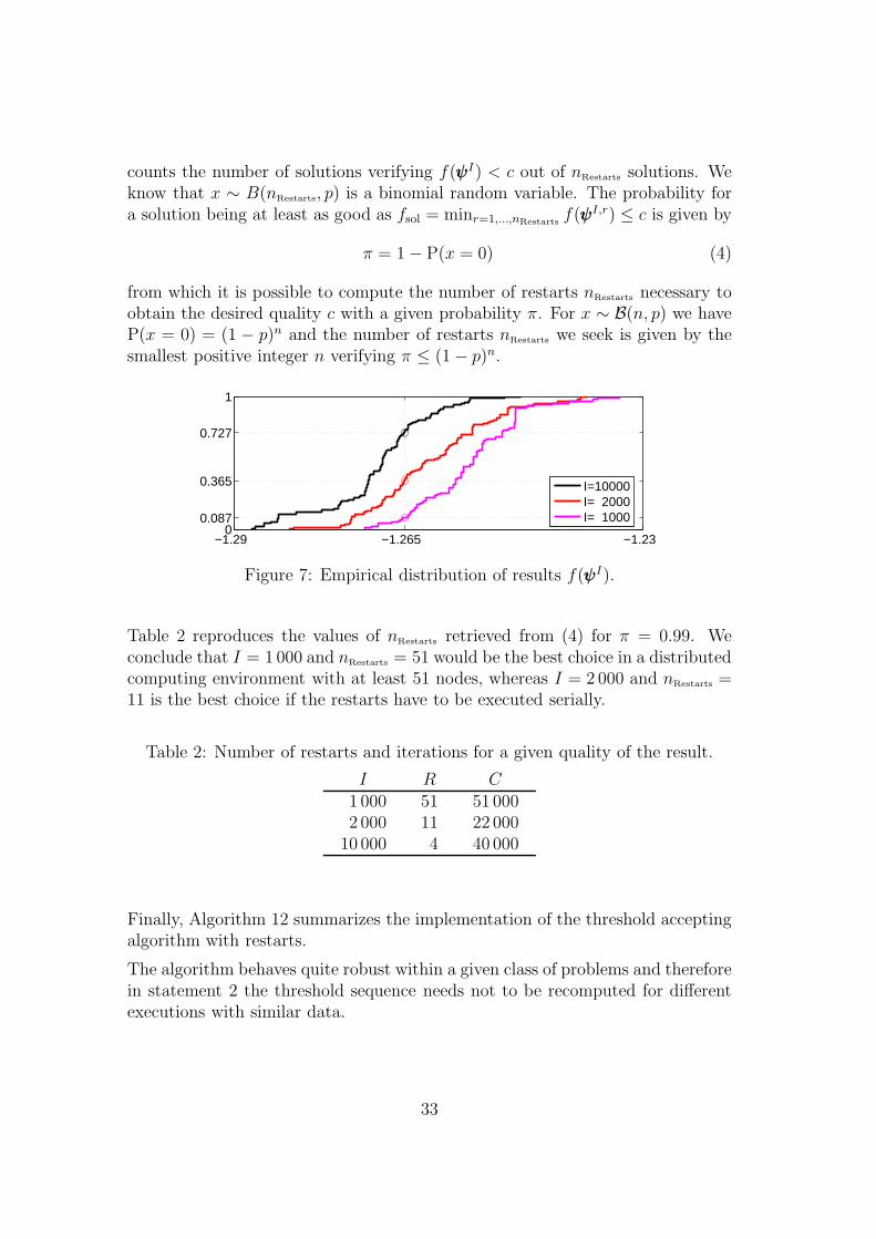
counts the number of solutions verifying f(ψψψI) < c out of nRestarts solutions. Weknow that x ∼ B(nRestarts, p) is a binomial random variable. The probability fora solution being at least as good as fsol = minr=1,...,nRestarts

f(ψψψI,r) ≤ c is given by

π = 1 − P(x = 0) (4)

from which it is possible to compute the number of restarts nRestarts necessary toobtain the desired quality c with a given probability π. For x ∼ B(n, p) we haveP(x = 0) = (1 − p)n and the number of restarts nRestarts we seek is given by thesmallest positive integer n verifying π ≤ (1 − p)n.

−1.29 −1.265 −1.230

0.087

0.365

0.727

1

I=10000I= 2000I= 1000

Figure 7: Empirical distribution of results f(ψψψI).

Table 2 reproduces the values of nRestarts retrieved from (4) for π = 0.99. Weconclude that I = 1 000 and nRestarts = 51 would be the best choice in a distributedcomputing environment with at least 51 nodes, whereas I = 2 000 and nRestarts =11 is the best choice if the restarts have to be executed serially.

Table 2: Number of restarts and iterations for a given quality of the result.

I R C1 000 51 51 0002 000 11 22 000

10 000 4 40 000

Finally, Algorithm 12 summarizes the implementation of the threshold acceptingalgorithm with restarts.

The algorithm behaves quite robust within a given class of problems and thereforein statement 2 the threshold sequence needs not to be recomputed for differentexecutions with similar data.

33

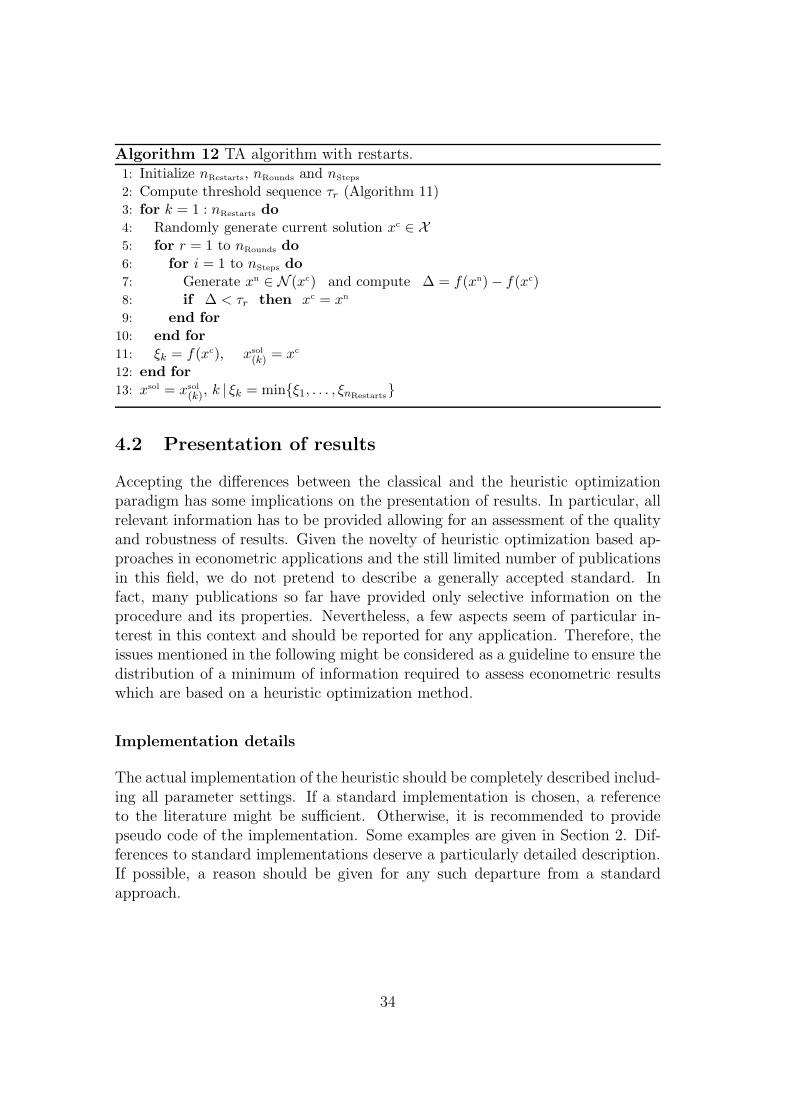
Algorithm 12 TA algorithm with restarts.1: Initialize nRestarts, nRounds and nSteps

2: Compute threshold sequence τr (Algorithm 11)3: for k = 1 : nRestarts do

4: Randomly generate current solution xc ∈ X5: for r = 1 to nRounds do

6: for i = 1 to nSteps do

7: Generate xn ∈ N (xc) and compute ∆ = f(xn) − f(xc)8: if ∆ < τr then xc = xn

9: end for

10: end for

11: ξk = f(xc), xsol

(k) = xc

12: end for

13: xsol = xsol

(k), k | ξk = minξ1, . . . , ξnRestarts

4.2 Presentation of results

Accepting the differences between the classical and the heuristic optimizationparadigm has some implications on the presentation of results. In particular, allrelevant information has to be provided allowing for an assessment of the qualityand robustness of results. Given the novelty of heuristic optimization based ap-proaches in econometric applications and the still limited number of publicationsin this field, we do not pretend to describe a generally accepted standard. Infact, many publications so far have provided only selective information on theprocedure and its properties. Nevertheless, a few aspects seem of particular in-terest in this context and should be reported for any application. Therefore, theissues mentioned in the following might be considered as a guideline to ensure thedistribution of a minimum of information required to assess econometric resultswhich are based on a heuristic optimization method.

Implementation details

The actual implementation of the heuristic should be completely described includ-ing all parameter settings. If a standard implementation is chosen, a referenceto the literature might be sufficient. Otherwise, it is recommended to providepseudo code of the implementation. Some examples are given in Section 2. Dif-ferences to standard implementations deserve a particularly detailed description.If possible, a reason should be given for any such departure from a standardapproach.

34

Pretesting

Typically, a preliminary test phase is run for choosing appropriate parameter val-ues for the heuristic. Preferably, this testing phase should follow some structuredapproach, e.g., a grid search over some parameter values. The approach followedshould be documented. In any case, it is relevant to report the number of runsin this preliminary phase as they will have an impact on the quality of the finaloutcomes.

Computational resources

Authors should always clearly indicate how much computational resources havebeen spent for each of the results presented. In general, stochastic algorithms willbe run repeatedly on a single problem instance. Then, the number of restartsand the number of iterations (generations) per restart should be indicated. Fur-thermore, information on the distribution of the results (in terms of values of theobjective function and/or other variables of interest, e.g., parameter estimates)should be provided. This might be done using standard statistics such as mean,variance and quantiles if only a small number of restarts has been considered, orby density plots similar to the example provided in Figure 4 in Section 3.1.

Rate of convergence

As long as an implementation of a heuristic does not provide the global opti-mum with probability close to one, an increase in computational resources spent(iterations/generations, restarts) should improve (expected) results. Since notheoretical results are available with regard to this convergence speed, empiricalinformation is highly valuable. It might be provided by some graphical presen-tation or an econometric estimate of the rate of convergence as presented for anexample in Section 3.2.

Generality of results

Finally, for comparison with other methods, results on a single problem instanceare not sufficient. Either multiple real problem instances should be discussed ora Monte Carlo simulation study should be conducted. In case of a Monte Carloanalysis, problem instances might be constructed in a way to allow for a responsesurface analysis of the results. Again, detailed information on the setup has tobe provided.

35

5 Selected applications

The selected applications presented in the following subsections are not meant topresent a complete analysis of the implementation of heuristics and the resultsobtained. Given the page constraint, they should rather provide an illustrationof some of the issues addressed in the previous sections, while not all of therequirements mentioned in Section 4.2 can be met.

The first example describes the discrete problem of model selection in VAR mod-els with an implementation of the threshold accepting heuristic. This examplehas been used to illustrate the stochastic dimension of working with optimizationheuristics in Section 3. The second example compares implementations of thresh-old accepting and differential evolution for the continuous optimization problemstemming from high breakdown point estimation.

5.1 Model selection in VAR models

A p-dimensional vector autoregressive process Xt is given by

Xt =

K∑

k=1

ΓΓΓkXt−k + εεεt , (5)

where εεεtiid∼ N(0,ΣΣΣ). The matrices ΓΓΓk provide the autoregression coefficients. In

the following, we assume that all component time series in Xt are stationary.For a more detailed treatment of this type of multivariate time series models,estimation issues and interpretation of results, the reader is referred to Lutkepohl(2007) in this volume.

Here, we assume that a maximum lag length K0 can be derived either fromeconomic theory or from some rule of thumb based on the number of availableobservations. Then, for a given realization of the process (X1, . . . ,XT ), the modelselection problem consists in identifying K along with those elements of ΓΓΓk, k =1, . . . , K, which are non zero in the process (5). Consequently, the search spacecan be described by the set Ω = 0, 1p2×K0, where a zero corresponds to aparameter constraint to be zero, and a one to a parameter to be estimated freely.

For this model selection problem, different objective functions can be considered.Information criteria represent one standard approach by weighting model fit (asmeasured by the determinant of the fitted residuals covariance matrix Σ) againstthe number of non zero parameters l. For the application presented in this sub-section, the Bayesian or Schwarz information criterion BIC = ln |Σ| + l lnT/Tis used (Schwarz, 1978). However, using a different information criterion doesnot require any change of the implementation besides replacing the objectivefunction.

36

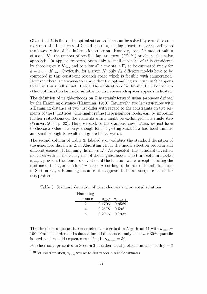
Given that Ω is finite, the optimization problem can be solved by complete enu-meration of all elements of Ω and choosing the lag structure corresponding tothe lowest value of the information criterion. However, even for modest valuesof p and K0, the number of possible lag structures (2p2×K0) precludes this naiveapproach. In applied research, often only a small subspace of Ω is consideredby choosing only Kmax and to allow all elements in ΓΓΓk to be estimated freely fork = 1, . . . , Kmax. Obviously, for a given K0 only K0 different models have to becompared in this constraint research space which is feasible with enumeration.However, there is no reason to expect that the optimal lag structure in Ω happensto fall in this small subset. Hence, the application of a threshold method or an-other optimization heuristic suitable for discrete search spaces appears indicated.

The definition of neighborhoods on Ω is straightforward using ε-spheres definedby the Hamming distance (Hamming, 1950). Intuitively, two lag structures witha Hamming distance of two just differ with regard to the constraints on two ele-ments of the Γ matrices. One might refine these neighborhoods, e.g., by imposingfurther restrictions on the elements which might be exchanged in a single step(Winker, 2000, p. 92). Here, we stick to the standard case. Then, we just haveto choose a value of ε large enough for not getting stuck in a bad local minimaand small enough to result in a guided local search.

The second column of Table 3, labeled σ∆N exhibits the standard deviation ofthe generated distances ∆ in Algorithm 11 for the model selection problem anddifferent choices of Hamming distances ε.21 As expected, this standard deviationincreases with an increasing size of the neighborhood. The third column labeledσaccepted provides the standard deviation of the function values accepted during theruntime of the algorithm for I = 5 000. According to the rule of thumb discussedin Section 4.1, a Hamming distance of 4 appears to be an adequate choice forthis problem.

Table 3: Standard deviation of local changes and accepted solutions.

Hammingdistance σ∆N σaccepted

2 0.1706 0.95694 0.2578 0.59616 0.2916 0.7932

The threshold sequence is constructed as described in Algorithm 11 with nSteps =100. From the ordered absolute values of differences, only the lower 30%-quantileis used as threshold sequence resulting in nRounds = 30.

For the results presented in Section 3, a rather small problem instance with p = 3

21For this simulation, nSteps was set to 500 to obtain reliable estimates.

37

andK = 3 has been considered. The problem instance exhibits different lag struc-tures for the three equations and “holes” such that the standard approach cannotresult in a proper model selection. The model selection procedure is applied tosimulated data from this process of length T = 100. For the optimization, we setK0 = 5.

When considering a single realization of the process, we find that the overall bestsolution is found 4 times for I = 500 iterations, 18 times for I = 1 000, 217times for I = 5 000 and 332 times for I = 10 000 iterations when consideringnRestarts = 1 000 restarts. At the same time, the mean relative deviation from thisbest solution decreases from 22% for I = 100 to 1.3% for I = 10 000 iterations.Given the low number of observations of the realization of the process, it shouldnot be expected that the model with the lowest value of the information criterionfound by the heuristic corresponds to the true data generating process. Theheuristic just delivers the best or at least a good approximation for the givenrealization.

Of course, a test of the properties of the presented application has to be basedon a much larger set of different model structures and realizations for a givenmodel structure. However, this is beyond the present contribution. More detailson model selection in VAR models including a much more comprehensive setof simulations can be found in Winker (2001, Ch. 12). A generalization of theapproach to non stationary time series, i.e. in a VEC modelling context is pre-sented by Winker and Maringer (2004) using a model selection criterion proposedby Chao and Phillips (1999) for (co)integrated series and the estimator proposedby Ahn and Reinsel (1990).22 According to their findings, adequate modelling ofthe autoregressive part of the model, e.g., by means of optimization heuristics,might have a strong impact on the correct identification of long run relationships.

5.2 High breakdown point estimation

We consider23 the linear regression model

yi =[

xi1 · · · xip

]

θ1...θp

+ ǫi i = 1, . . . , n (6)

where θ ∈ Rp are the parameters and ǫ ∼ N(0, σ2I) is the disturbance vector. The

breakdown point of an estimator is defined as the smallest percentage of conta-mination in the data that may cause the estimator to be affected by an arbitrary

22Bauer and Wagner (2002) propose an alternative estimator which might also be used inthe context of model selection for (co)integrated time series.

23Builds on a presentation given by M. Gilli and A. Marazzi at the 3rd IASC World conferencein Limassol, Cyprus, 28–31 October 2005.

38

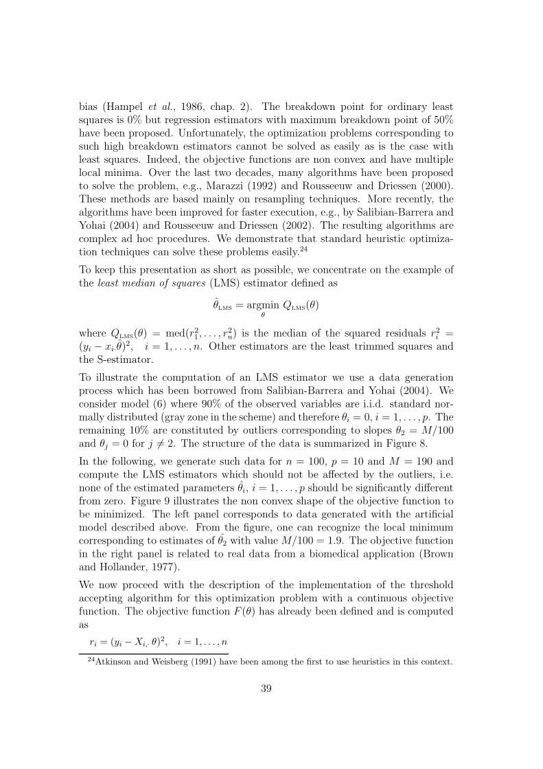
bias (Hampel et al., 1986, chap. 2). The breakdown point for ordinary leastsquares is 0% but regression estimators with maximum breakdown point of 50%have been proposed. Unfortunately, the optimization problems corresponding tosuch high breakdown estimators cannot be solved as easily as is the case withleast squares. Indeed, the objective functions are non convex and have multiplelocal minima. Over the last two decades, many algorithms have been proposedto solve the problem, e.g., Marazzi (1992) and Rousseeuw and Driessen (2000).These methods are based mainly on resampling techniques. More recently, thealgorithms have been improved for faster execution, e.g., by Salibian-Barrera andYohai (2004) and Rousseeuw and Driessen (2002). The resulting algorithms arecomplex ad hoc procedures. We demonstrate that standard heuristic optimiza-tion techniques can solve these problems easily.24

To keep this presentation as short as possible, we concentrate on the example ofthe least median of squares (LMS) estimator defined as

θLMS = argminθ

QLMS(θ)

where QLMS(θ) = med(r21, . . . , r

2n) is the median of the squared residuals r2

i =(yi − xi·θ)

2, i = 1, . . . , n. Other estimators are the least trimmed squares andthe S-estimator.

To illustrate the computation of an LMS estimator we use a data generationprocess which has been borrowed from Salibian-Barrera and Yohai (2004). Weconsider model (6) where 90% of the observed variables are i.i.d. standard nor-mally distributed (gray zone in the scheme) and therefore θi = 0, i = 1, . . . , p. Theremaining 10% are constituted by outliers corresponding to slopes θ2 = M/100and θj = 0 for j 6= 2. The structure of the data is summarized in Figure 8.

In the following, we generate such data for n = 100, p = 10 and M = 190 andcompute the LMS estimators which should not be affected by the outliers, i.e.none of the estimated parameters θi, i = 1, . . . , p should be significantly differentfrom zero. Figure 9 illustrates the non convex shape of the objective function tobe minimized. The left panel corresponds to data generated with the artificialmodel described above. From the figure, one can recognize the local minimumcorresponding to estimates of θ2 with value M/100 = 1.9. The objective functionin the right panel is related to real data from a biomedical application (Brownand Hollander, 1977).

We now proceed with the description of the implementation of the thresholdaccepting algorithm for this optimization problem with a continuous objectivefunction. The objective function F (θ) has already been defined and is computedas

ri = (yi − Xi,· θ)2, i = 1, . . . , n

24Atkinson and Weisberg (1991) have been among the first to use heuristics in this context.

39

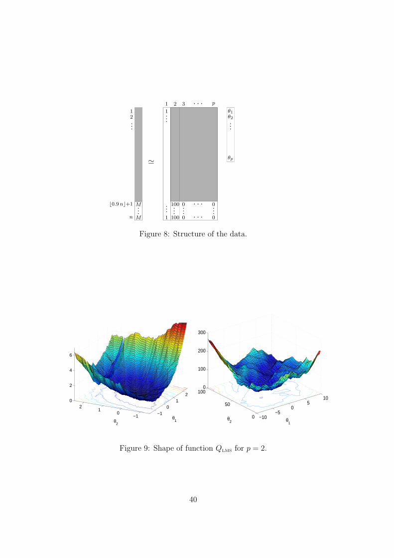
M...M

12...

⌊0.9 n⌋+1

n

≃

1...

...1

100...100

1 2 3 · · · p

0...0

0· · · ...0· · ·

θ1

θ2

...

θp

Figure 8: Structure of the data.

−10

12

−10

12

0

2

4

6

θ1θ

2

−10−5

05

10

0

50

1000

100

200

300

θ1

θ2

Figure 9: Shape of function QLMS for p = 2.

40

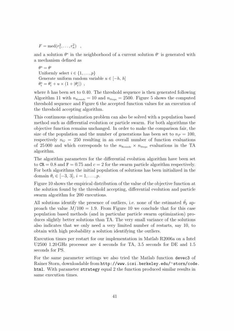
F = med(r21, . . . , r

2n) ,

and a solution θn in the neighborhood of a current solution θc is generated witha mechanism defined as

θn = θc

Uniformly select i ∈ 1, . . . , pGenerate uniform random variable u ∈ [−h, h]θn

i = θc

i + u × (1 + |θc

i |) ,

where h has been set to 0.40. The threshold sequence is then generated followingAlgorithm 11 with nRounds = 10 and nSteps = 2500. Figure 5 shows the computedthreshold sequence and Figure 6 the accepted function values for an execution ofthe threshold accepting algorithm.

This continuous optimization problem can also be solved with a population basedmethod such as differential evolution or particle swarm. For both algorithms theobjective function remains unchanged. In order to make the comparison fair, thesize of the population and the number of generations has been set to nP = 100,respectively nG = 250 resulting in an overall number of function evaluationsof 25 000 and which corresponds to the nRounds × nSteps evaluations in the TAalgorithm.

The algorithm parameters for the differential evolution algorithm have been setto CR = 0.8 and F = 0.75 and c = 2 for the swarm particle algorithm respectively.For both algorithms the initial population of solutions has been initialized in thedomain θi ∈ [−3, 3], i = 1, . . . , p.

Figure 10 shows the empirical distribution of the value of the objective function atthe solution found by the threshold accepting, differential evolution and particleswarm algorithm for 200 executions.

All solutions identify the presence of outliers, i.e. none of the estimated θ2 ap-proach the value M/100 = 1.9. From Figure 10 we conclude that for this casepopulation based methods (and in particular particle swarm optimization) pro-duces slightly better solutions than TA. The very small variance of the solutionsalso indicates that we only need a very limited number of restarts, say 10, toobtain with high probability a solution identifying the outliers.

Execution times per restart for our implementation in Matlab R2006a on a IntelU2500 1.20GHz processor are 4 seconds for TA, 3.5 seconds for DE and 1.5seconds for PS.

For the same parameter settings we also tried the Matlab function devec3 ofRainer Storn, downloadable from http://www.icsi.berkeley.edu/∼storn/code.

html. With parameter strategy equal 2 the function produced similar results insame execution times.

41

0.25 0.3 0.35 0.4 0.450

0.5

1

PS DE TA

Figure 10: Empirical distribution of the value of the objective function of 200solutions for TA, DE and PS.

6 Conclusions

In this contribution, the use of optimization heuristics in econometrics is moti-vated by the fact that many optimization problems in econometrics cannot bedealt with adequately using classical tools. Instead of simplifying the model,searching for alternative work arounds or using highly specified algorithms, wepropose to employ general optimization heuristics.

The chapter provides an overview of some of the most commonly used optimiza-tion heuristics in fields close to econometrics, e.g., in statistics and finance. Fur-thermore, a classification of the basic algorithms and possible hybrids providesa base for selection of algorithms which might be most suitable for a specificproblem instance.

In traditional applications of optimization heuristics in operations research, engi-neering and related fields, the inherent randomness of the results does not seemto play a major role. However, econometricians appear to be very anxious aboutthis stochastic component. Therefore, a formal approach is proposed to deal withthis additional source of randomness in the context of econometric applications.Obviously, our contribution provides only a few preliminary insights and mightpoint towards issues deserving additional research. Nevertheless, the results pre-sented indicate that it might be possible to include the randomness stemmingfrom the application of optimization heuristics in the usual econometric analysis.

Another major obstacle to a more widespread use of optimization heuristics ap-pears to be that few standard applications are available and most algorithmsrequire some parameter tuning for a specific problem instance. In a chapter de-voted to implementation issues, we tried to summarize our (limited) knowledgeabout these issues and to provide guidelines to the potential user of such meth-ods. According to our understanding, it is equally important for a more generaluse of the heuristic methods that authors and editors become more careful aboutthe presentation of the results. Again, we presented some guidelines without

42

claiming that they represent a complete set.

The chapter is complemented by the short description of two applications ineconometrics, one for a discrete optimization problem in model selection and thesecond for a continuous optimization problem. The results indicate that thesemethods represent a valuable extension of the econometrician’s toolbox when itcomes to model and estimate slightly more complex problems than standard linearleast squares. We are confident that given their performance, the methods willbecome a standard tool once a common standard for presentation and evaluationof the results and their randomness has been developed and is generally accepted.

References

Aarts, E. and J. Korst (1989). Simulated Annealing and Boltzmann Machines. J.Wiley and Sons. Chichester.

Acosta-Gonzalez, E. and F. Fernandez-Rodrıguez (2007). Model selection via ge-netic algorithms illustrated with cross-country growth data. Empirical Eco-nomics 33, 313–337.

Adanu, K. (2006). Optimizing the GARCH model – an application of two globaland two local search methods. Computational Economics 28, 277–290.

Ahn, S.K. and G.C. Reinsel (1990). Estimation for partially nonstationary mul-tivariate autoregressive models. Journal of the American Statistical Associ-ation 85(411), 813–823.

Alcock, J. and K. Burrage (2004). A genetic estimation algorithm for parametersof stochastic ordinary differential equations. Computational Statistics andData Anylsis 47(2), 255–275.

Althofer, I. and K.-U. Koschnik (1991). On the convergence of threshold accept-ing. Applied Mathematics and Optimization 24, 183–195.

Atkinson, A.C. and S.W. Weisberg (1991). Simulated annealing for the detectionof multiple outliers using least squares and least median of squares fitting.In: Directions in robust statistics and diagnostics, Part I (W.A.Stahel andS.W. Weisberg, Ed.). Springer-Verlag. New York.

Baragona, R., F. Battaglia and C. Calzini (2001). Genetic algorithms for the iden-tification of additive and innovation outliers in time series. ComputationalStatistics & Data Analysis 37(1), 1–12.

43

Baragona, R., F. Battaglia and D. Cucina (2004). Fitting piecewise linear thresh-old autoregressive models by means of genetic algorithms. ComputationalStatistics & Data Analysis 47, 277–295.

Bauer, D. and M. Wagner (2002). Estimating cointegrated systems using subspacealgorithms. Journal of Econometrics 111, 47–84.

Birattari, M., L. Paquete, T. Stutzle and K. Varrentrap (2001). Classificationof metaheuristics and design of experiments for the analysis of components.Technical Report AIDA-2001-05. Intellektik, Technische Universitat Darm-stadt, Germany.

Bock, F. (1958). An algorithm for solving “traveling salesman” and related net-work optimization problems. 14th ORSA meeting, St. Louis.

Brooks, S.P. and B.J.T. Morgan (1995). Optimization using simulated annealing.The Statistician 44(2), 241–257.

Brooks, S.P., N. Friel and R. King (2003). Classical model selection via simulatedannealing. Journal of the Royal Statistical Society Series B 65, 503–520.

Brown, B.W. and M. Hollander (1977). Statistics: A Biomedical Introduction.Wiley. New York.

Chao, J.C. and P.C.B. Phillips (1999). Model selection in partially nonstation-ary vector autoregressive processes with reduced rank structure. Journal ofEconometrics 91, 227–271.

Chipman, J. S. and P. Winker (2005). Optimal aggregation of linear time seriesmodels. Computational Statistics and Data Analysis 49(2), 311–331.

Colorni, A., M. Dorigo and V. Manniezzo (1992a). Distributed optimization byant colonies. In: Proceedings of the First European Conference on Artifi-cial Life (ECAL-91) (F.J. Varela and P. Bourgine, Ed.). The MIT Press.Cambridge MA. pp. 134–142.

Colorni, A., M. Dorigo and V. Manniezzo (1992b). An investigation of someproperties of an ant algorithm. In: Parallel problem solving from nature,Vol 2. (R. Manner and B. Manderick, Ed.). North-Holland. Amsterdam.pp. 509–520.

Cormen, T.H., C.E. Leiserson and R.L. Rivest (1990). Introduction to Algorithms.MIT Electrical Engineering and Computer Science. MIT Press. Cambridge.

Croes, G.A. (1958). A method for solving traveling salesman problems. OperationsResearch 6, 791–812.

44

Dempster, A.P., N.M. Laird and D.B. Rubin (1977). Maximum likelihood fromincomplete data via the EM algorithm. J. Roy. Statist. Soc. Ser. B 39, 1–38.

Doornik, J.A. and M. Ooms (2003). Multimodality in the GARCH regressionmodell. Technical Report 2003-W20. University of Oxford. Oxford.

Dorsey, B. and W.J. Mayer (1995). Genetic algorithms for estimation problemswith multiple optima, nondifferentiability and other irregular features. Jour-nal of Business and Economic Statistics 13, 53–66.

Dueck, G. (1993). New optimization heuristics: The great-deluge algorithm andthe record-to-record travel. Journal of Computational Physics 13, 53–66.

Dueck, G. and T. Scheuer (1990). Threshold accepting: A general purpose algo-rithm appearing superior to simulated annealing. Journal of ComputationalPhysics 90, 161–175.

Eberhart, R.C. and J. Kennedy (1995). A new optimizer using particle swarmtheory. In: Proceedings of the Sixth International Symposium on Microma-chine and Human Science. Nagoya, Japan. pp. 39–43.

Fang, K.-T., D. Maringer, Y. Tang and P. Winker (2005). Lower bounds andstochastic optimization algorithms for uniform designs with three or fourlevels. Mathematics of Computation 75(254), 859–878.

Fang, Kai-Tai, Xuan Lu and P. Winker (2003). Lower bounds for centered andwrap–around l2–discrepancies and construction of uniform designs by thresh-old accepting. Journal of Complexity 19, 692–711.

Fitzenberger, B. and P. Winker (2007). Improving the computation of censoredquantile regressions. Computational Statistics & Data Analysis 52(1), 88–108.

Gan, L. and J. Jiang (1999). A test for global maximum. Journal of the AmericanStatistical Association 94(447), 847–854.

Glover, F. and M. Laguna (1997). Tabu Search. Kluwer Academic Publishers.Boston, MA.

Goffe, W.L., G.D. Ferrier and J. Rogers (1994). Global optimization of statisticalfunctions with simulated annealing. Journal of Econometrics 60(1-2), 65–99.

Hamming, R.W. (1950). Error detecting and error correcting codes. Bell SystemTechnical Journal 29, 147–160.

Hampel, F.R., E.M. Ronchetti, P.J. Rousseeuw and W.A. Stahel (1986). RobustStatistics: The Approach based on Influence Functions. Wiley. New York.

45

Hawkins, D.S., D.M. Allen and A.J. Stromberg (2001). Determining the numberof components in mixtures of linear models. Computational Statistics & DataAnalysis 38(1), 15–48.

Holland, J.H. (1975). Adaptation in Natural and Artificial Systems. The Univer-sity of Michigan Press. Ann Arbor, MI.

Hoos, H.H. and T. Stutzle (2005). Stochastic Local Search: Foundations andApplications. Elsevier. Amsterdam.

Husler, J., P. Cruz, A. Hall and C.M. Fonseca (2003). On optimization andextreme value theory. Methodology and Computing in Applied Probability5, 183–195.

Jacobson, S.H. and E. Yucesan (2004). Global optimization performance mea-sures for generalized hill climbing algorithms. Journal of Global Optimization29, 173–190.

Jacobson, S.H., S.N. Hall and L.A. McLay (2006). Visiting near-optimal solu-tions using local search algorithms. In: COMPSTAT 2006, Proceedings inComputational Statistics (Alfredo Rizzi and Maurizio Vichi, Ed.). Physica.Heidelberg. pp. 471–481.

Jerrell, M.E. and W.A. Campione (2001). Global optimization of econometricfunctions. Journal of Global Optimization 20(3-4), 273–295.

Kapetanios, G. (2007). Variable selection in regression models using nonstan-dard optimisation of information criteria. Computational Statistics & DataAnalysis 52(1), 4–15.

Kapetanios, George (2006). Choosing the optimal set of instruments from largeinstrument sets. Computational Statistics & Data Analysis 51(2), 612–620.

Lourenco, H.R., O. Martin and T. Stutzle (2002). Iterated local search. In: Hand-book of Metaheuristics (F. Glover and G. Kochenberger, Ed.). Vol. 57 of In-ternational Series in Operations Research and Management Science. KluwerAcademic Publishers. Norwell, MA. pp. 321–353.

Lutkepohl, H. (2007). Econometric analysis with vector autoregressive models.In: Handbook of Computational Econometrics (E. Konthoghiorghes et al.,Eds.). Elsevier. Amsterdam. p. forthcomming.

Maddala, G.S. and F.D. Nelson (1974). Maximum likelihood methods for modelsof markets in disequilibrium. Econometrica 42(6), 303–317.

Marazzi, A. (1992). Algorithms, Routines and S-functions for Robust Statistics.Wadsworth & Brooks/Cole.

46

Maringer, D. (2005). Portfolio Management with Heuristic Optimization.Springer. Dordrecht.

Maringer, D. and M. Meyer (2006). Smooth transition autoregressive models –new approaches to the model selection problem. Technical Report WP010-06. University of Essex. Colchester.

Maringer, D. and P. Winker (2006). The convergence of optimization basedGARCH estimators: Theory and application. In: COMPSTAT 2006, Pro-ceedings in Computational Statistics (Alfredo Rizzi and Maurizio Vichi, Ed.).Physica. Heidelberg. pp. 483–494.

Mladenovic, N. and P. Hansen (1997). Variable neighborhood search. Computersand Operations Research 34, 1097–1100.

Moscato, P. (1989). On evolution, search, optimization, genetic algorithms andmartial arts: Towards memetic algorithms. Technical report. Caltech.

Osman, I. H. and G. Laporte (1996). Metaheuristics: A bibliography. Annals ofOperations Research 63, 513–623.

Reeves, C.R. and J.E. Rowe (2003). Genetic Algorithms – Principles and Per-spectives. Kluwer. Boston.

Rousseeuw, P.J. and K. Van Driessen (2000). An algorithm for positive-breakdown regression based on concentration steps. In: Data Analysis:Scientific Modeling and Practical Application (W. Gaul, O. Opitz andM. Schader, Ed.). Springer-Verlag. Berlin. pp. 335–346.

Rousseeuw, P.J. and K. Van Driessen (2002). Computing LTS regression for largedata sets. Estadistica 54, 163–190.

Rudolph, G. (1997). Convergence Properties of Evolutionary Algorithms. Kovac.Hamburg.

Salibian-Barrera, M. and V.J. Yohai (2004). A fast algorithm for S-regressionestimates. Technical report. University of British Columbia.

Schwarz, G. (1978). Estimating the dimension of a model. The Annals of Statistics6, 461–464.

Staszewska, A. (2007). Representing uncertainty about response paths: The useof heuristic optimisation methods. Computational Statistics & Data Analysis52(1), 121–132.

Storn, R. and K. Price (1997). Differential evolution – a simple and efficientheuristic for global optimization over continuous spaces. Journal of GlobalOptimization 11, 341–359.

47

Taillard, E.D., L.M. Gambardella, M. Gendreau and J-Y. Potvin (2000). Adap-tive memory programming: A unified view of metaheuristics. European Jour-nal of Operational Research 135, 1–16.

Talbi, E-G. (2002). A taxonomy of hybrid metaheuristics. Journal of Heuristics8, 541–564.

Winker, P. (1995). Identification of multivariate AR-models by threshold accept-ing. Computational Statistics and Data Analysis 20(9), 295–307.

Winker, P. (2000). Optimized multivariate lag structure selection. ComputationalEconomics 16, 87–103.

Winker, P. (2001). Optimization Heuristics in Econometrics: Applications ofThreshold Accepting. Wiley. Chichester.

Winker, P. and D. Maringer (2004). Optimal lag structure selection in VARand VEC models. In: New Directions in Macromodeling (A. Welfe, Eds.).Elsevier. Amsterdam. pp. 213–234.

Winker, P. and D. Maringer (2007). The threshold accepting optimisation algo-rithm in economics and statistics. In: Optimisation, Econometric and Finan-cial Analysis (E. J. Kontoghiorghes and C. Gatu, Ed.). Vol. 9 of Advancesin Computational Management Science. Springer. Berlin. pp. 107–125.

Winker, P. and Kai-Tai Fang (1997). Application of threshold accepting to theevaluation of the discrepancy of a set of points. SIAM Journal on NumericalAnalysis 34, 2028–2042.

Yang, Z., Z. Tian and Z. Yuan (2007). GSA-based maximum likelihood estimationfor threshold vector error correction model. Computational Statistics & DataAnalysis 52(1), 109–120.

48