Heterogeneous Convergence - Emory University

Heterogeneous Convergence

Andrew T. Young a,, Matthew J. Higgins b, Daniel Levy c

a College of Business and Economics, West Virginia University

Morgantown, WV 26505, USA

b College of Management, Georgia Institute of Technology Atlanta, GA 30308, USA

c Department of Economics, Bar-Ilan University Ramat-Gan 52900, ISRAEL

Department of Economics, Emory University Atlanta, GA 30322, USA

and RCEA, University of Bologna

Rimini, ITALY ______________________________________________________________________________________ Abstract We use U.S. county-level data containing 3,058 cross-sectional observations and 41 conditioning variables to study economic growth and explore possible heterogeneity in growth determination across 32 individual states. Using a 3SLS-IV estimation method, we find that all statistically significant convergence rates (for 32 individual states) are above 2 percent, with an average of 8.1 percent. For 7 states the convergence rate can be rejected as identical to at least one other state’s convergence rate with 95 percent confidence. Convergence rates are negatively correlated with initial income. The size of government at all levels of decentralization is either unproductive or negatively correlated with growth. Educational attainment has a non-linear relationship with growth. The size of the finance, insurance and real estate, and entertainment industries are positively correlated with growth, while the size of the education industry is negatively correlated with growth. Heterogeneity in the effects of balanced growth path determinants across individual states is harder to detect than in convergence rates.

JEL Codes: O40, O11, O18, O51, R11, H50, H70

Key Words: Economic Growth, Conditional Convergence, County Level Data _________________________________________________________________________

We thank Steven Durlauf, Jordan Rappaport and Jerry Thursby for helpful comments and suggestions. We are grateful to Jordan Rappaport for kindly sharing with us data and computer codes. The second author acknowledges financial assistance from a National Science Foundation IGERT Fellowship. All remaining errors are our own.

Corresponding author: [email protected]

1

1. Introduction

Empirical studies of conditional convergence implicitly assume that all economies

have identically-structured growth processes and, therefore, it is meaningful to estimate a

single rate of convergence for them. See, for example, Barro and Sala-i-Martin (1991,

1992), Mankiw et al. (1992), Islam (1995), and Caselli et al. (1996). However, Evans

(1998) and Brock and Durlauf (2001) emphasize that this assumption is not plausible for

most data sets because "countries surely have different technologies, preferences,

institutions, market structures, government policies, etc" (Evans, 1998, p. 296). These

can represent important structural differences.1

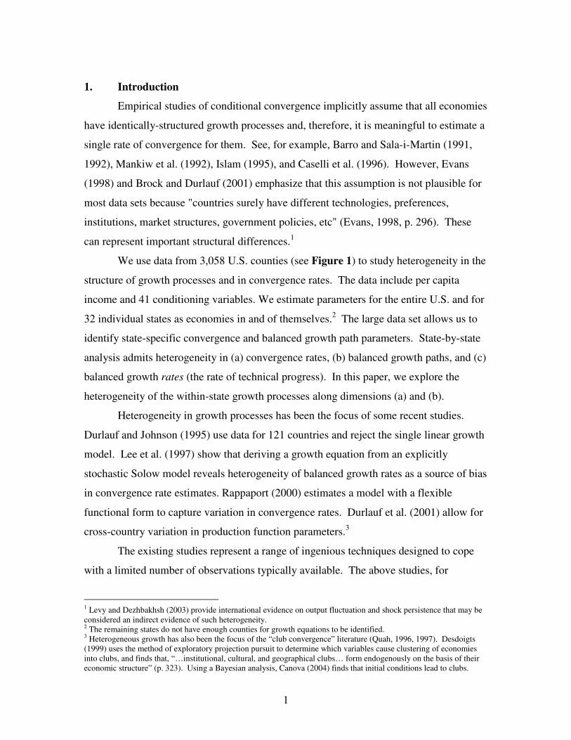
We use data from 3,058 U.S. counties (see Figure 1) to study heterogeneity in the

structure of growth processes and in convergence rates. The data include per capita

income and 41 conditioning variables. We estimate parameters for the entire U.S. and for

32 individual states as economies in and of themselves.2 The large data set allows us to

identify state-specific convergence and balanced growth path parameters. State-by-state

analysis admits heterogeneity in (a) convergence rates, (b) balanced growth paths, and (c)

balanced growth rates (the rate of technical progress). In this paper, we explore the

heterogeneity of the within-state growth processes along dimensions (a) and (b).

Heterogeneity in growth processes has been the focus of some recent studies.

Durlauf and Johnson (1995) use data for 121 countries and reject the single linear growth

model. Lee et al. (1997) show that deriving a growth equation from an explicitly

stochastic Solow model reveals heterogeneity of balanced growth rates as a source of bias

in convergence rate estimates. Rappaport (2000) estimates a model with a flexible

functional form to capture variation in convergence rates. Durlauf et al. (2001) allow for

cross-country variation in production function parameters.3

The existing studies represent a range of ingenious techniques designed to cope

with a limited number of observations typically available. The above studies, for

1 Levy and Dezhbakhsh (2003) provide international evidence on output fluctuation and shock persistence that may be

considered an indirect evidence of such heterogeneity. 2 The remaining states do not have enough counties for growth equations to be identified. 3 Heterogeneous growth has also been the focus of the “club convergence” literature (Quah, 1996, 1997). Desdoigts

(1999) uses the method of exploratory projection pursuit to determine which variables cause clustering of economies

into clubs, and finds that, “…institutional, cultural, and geographical clubs… form endogenously on the basis of their

economic structure” (p. 323). Using a Bayesian analysis, Canova (2004) finds that initial conditions lead to clubs.

2

example, depart from the convergence literature by innovating primarily along the lines

of econometric specification. The present paper uses new data as its primary innovation.

Given our unusually large data set covering the entire U.S., we are able to explore

heterogeneity in convergence rates across the U.S. and amongst the majority of its states

without the need of any special econometric method for capturing the heterogeneity.

Besides the large number of observations and conditioning variables, our county

data offer several advantages. A single institution collects the data, ensuring uniformity

of variable definitions. There is no exchange rate variation between the counties and the

price variation across counties is smaller than across countries, reducing the potential

errors-in-variables bias (Bliss, 1999).4 Importantly, counties within a given state form a

sample with geographical homogeneity and a shared state government. To a great extent

the states are ready-made “clubs” within which we would expect convergence. The large

data set allows us to study inter-state heterogeneity, while the intra-state homogeneity

gives as much assurance of a correct specification as can realistically be hoped for.

Lastly of note is the relative homogeneity of U.S. counties as a whole. If we find

economically important heterogeneity of growth processes across states, then surely we

can infer that as much, or (likely) more, heterogeneity exists across countries.

Following Higgins et al. (2006) we use a cross-sectional variant of a 3SLS-IV

approach first developed by Evans (1997b) for estimating the growth equations. Evans

(1997b) and Caselli et al. (1996) show that data must satisfy highly implausible

conditions for OLS estimators to be consistent. Caselli et al. suggest a panel GMM

method that differences out omitted variable bias and uses instruments to alleviate

endogeneity concerns. This method, however, is useful if there are enough time series

observations after differencing. In our data, most of the conditioning variables come

from the U.S. Census and, therefore, are collected only at 10 year intervals. Our data’s

appeal lies in the exceptionally large cross-sectional dimension and, therefore, a cross-

sectional estimation technique appears more appropriate.5

We find significant heterogeneity in the state-level convergence rates. Across the

4 These virtues are also embodied in state-level data used by Barro and Sala-i-Martin (1991) and Evans (1997a). State-

level data, however, sacrifices the large number of observations we have. A full 29 of our states have counties

numbering more than 50 (the number of U.S. states) each. 5 Evans (1997a) develops a panel data variant of his method and applies it to U.S. state and international data, obtaining

convergence rate estimates of 16 and 6 percent, respectively.

3

32 states, 3SLS point estimates range from 3.8 percent (California) to 15.6 percent

(Louisiana), with an average of 8.1 percent. The 95 percent confidence intervals

associated with these estimates are narrow; heterogeneity cannot be merely dismissed on

grounds of statistical uncertainty. We find a statistically significant, but small, negative

partial correlation between the convergence rate and initial income, suggesting that

(initially) poorer states are not facing relatively poor convergence potentials. We also

find that the size of government at all levels of decentralization is either unproductive or

negatively correlated with growth. Educational attainment has a non-linear relationship

with growth. The size of the finance, insurance and real estate, and the entertainment

industries are positively correlated with growth, while the size of the education service

sector is negatively correlated with growth. Finally, heterogeneity in the effects of

balanced growth path determinants across U.S. states is harder to detect than in

convergence rates.

The paper is organized as follows. Section 2 discusses the model and the 3SLS

method; section 3 describes the data; section 4 studies heterogeneity in the convergence

rates; section 5 focuses on balanced growth path determinants; section 6 discusses model

uncertainty; and section 7 concludes.

2. The Model and 3SLS Estimation Procedure

The basic specification used in growth regressions arises from the neoclassical

growth model.6 The growth model implies that,

(2.1) )1(ˆ)0(ˆ)(ˆ * BtBt eyeyty −− −+=

where y is the log of income per effective unit of labor, t denotes the time, and B is a

nonlinear function of various parameters (preference parameters, population growth rate,

etc). B governs the speed of adjustment to the steady state, *y . From (2.1) it follows that

the average growth rate of income per unit of labor between dates 0 and T is,

6 A derivation of the baseline specification is provided by Barro and Sala-i-Martin (1992).

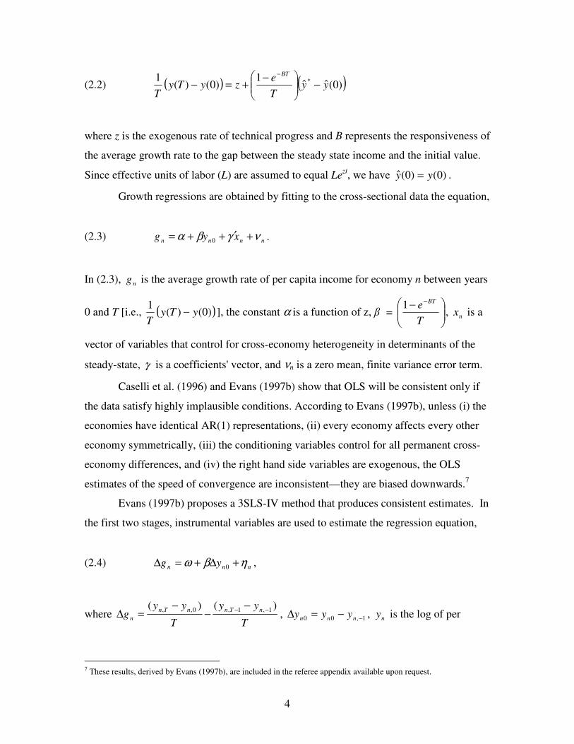
4

(2.2) ( ) ( ))0(ˆˆ1

)0()(1 *

yyT

ezyTy

T

BT

−

−+=−

−

where z is the exogenous rate of technical progress and B represents the responsiveness of

the average growth rate to the gap between the steady state income and the initial value.

Since effective units of labor (L) are assumed to equal Lezt, we have )0()0(ˆ yy = .

Growth regressions are obtained by fitting to the cross-sectional data the equation,

(2.3) nnnn xyg νγβα +′++= 0 .

In (2.3), ng is the average growth rate of per capita income for economy n between years

0 and T [i.e., ( ))0()(1

yTyT

− ], the constant α is a function of z, β =

− −

T

e BT1, nx is a

vector of variables that control for cross-economy heterogeneity in determinants of the

steady-state, γ is a coefficients' vector, and νn is a zero mean, finite variance error term.

Caselli et al. (1996) and Evans (1997b) show that OLS will be consistent only if

the data satisfy highly implausible conditions. According to Evans (1997b), unless (i) the

economies have identical AR(1) representations, (ii) every economy affects every other

economy symmetrically, (iii) the conditioning variables control for all permanent cross-

economy differences, and (iv) the right hand side variables are exogenous, the OLS

estimates of the speed of convergence are inconsistent—they are biased downwards.7

Evans (1997b) proposes a 3SLS-IV method that produces consistent estimates. In

the first two stages, instrumental variables are used to estimate the regression equation,

(2.4) nnn yg ηβω +∆+=∆ 0 ,

where T

yy

T

yyg

nTnnTn

n

)()( 1,1,0,, −− −−

−=∆ , 1,00 −−=∆ nnn yyy , ny is the log of per

7 These results, derived by Evans (1997b), are included in the referee appendix available upon request.

5

capita income for county n, ω and β are parameters, and nη is the error.8 ,9

As

instruments we use the lagged (1969) values of all nx variables except Metro, Per-Capita

Water Area, and Per-Capita Land Area.10

Given our sample period, we define:

∆gn =(y

n,1998 − yn,1970)

T−

(yn,1997 − y

n,1969)

T.

Next, we use *β , the estimate from (2.4), to construct the variable

(2.5) 0

*

nnn yg βπ −= .

In the third stage, we use the OLS to regress nπ on the vector nx , which consists of the

potential determinants of the balanced growth path levels. That is,

(2.6) nnn x εγτπ ++= ,

where τ and γ are parameters and εn is the error term. This regression yields a consistent

estimator, γ*.11

Also note that in principle τ is the same as the OLS α: it is an estimate of

the exogenous rate of technical progress, z, or the balanced growth rate.

Thus, to briefly summarize the 3SLS procedure we use, in the first two stages, it

differences out any uncontrolled form of heterogeneity to eliminate omitted variable bias

8 An immediate concern with the use of (2.4) is the reliance on the information from the single difference in the level of

income (1969 to 1970) to explain the difference in average growth rates over overlapping time periods (1969 to 1997

and 1970 to 1998). Given that the growth determination is a stochastic process, the potential problem is basically one

of a high noise to signal ratio. We are relying on large degrees of freedom to alleviate this problem and identify the

convergence rates. Indeed, as reported below, we obtain statistically significant convergence rate estimates for the full

sample as well as for all 32 individual states. 9 As Evans (1997b) shows, the derivation of this equation depends on the assumption that the xn variables are constant

during the time frame considered, allowing them to be differenced out. Since the difference is only over a single year

and these are variables representing broad demographic trends, this does not seem to be unwarranted. To make sure

that this did not introduce significant omitted variable bias into our estimations, we ran the IV regression for the full

U.S. sample with differenced values of all conditioning variables included as regressors. The point estimate of β from

the modified IV fell within the 95 percent confidence interval of the Evans IV method estimate. If β estimates are not

significantly affected then neither are the third stage results (see below). 10 See the data appendix for details and Table 1 for the list of the conditioning variables. 11 Technically speaking, γ is not the partial effects of xn variables on the heights of the balanced growth paths. Those

partial effects are functions of β and γ. However, if the neoclassical growth hypothesis is true (β < 0), then signs of

elements of γ will be the same as those of the partial effects of given xn elements. Assuming that β is identical across

economies, the size of γ elements relative to one another expresses the magnitude of the partial effects relative to one

another. Thus, while γ* does not allow for precise quantitative statements about the effects of given variables on

balanced growth paths, it does allow for statements about the sign of such effects, and how important those effects are

relative to each other.

6

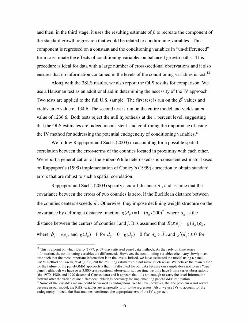
and then, in the third stage, it uses the resulting estimate of β to recreate the component of

the standard growth regression that would be related to conditioning variables. This

component is regressed on a constant and the conditioning variables in “un-differenced”

form to estimate the effects of conditioning variables on balanced growth paths. This

procedure is ideal for data with a large number of cross-sectional observations and it also

ensures that no information contained in the levels of the conditioning variables is lost.12

Along with the 3SLS results, we also report the OLS results for comparison. We

use a Hausman test as an additional aid in determining the necessity of the IV approach.

Two tests are applied to the full U.S. sample. The first test is run on the β* values and

yields an m value of 134.6. The second test is run on the entire model and yields an m

value of 1236.6. Both tests reject the null hypothesis at the 1 percent level, suggesting

that the OLS estimates are indeed inconsistent, and confirming the importance of using

the IV method for addressing the potential endogeneity of conditioning variables.13

We follow Rappaport and Sachs (2003) in accounting for a possible spatial

correlation between the error-terms of the counties located in proximity with each other.

We report a generalization of the Huber-White heteroskedastic-consistent estimator based

on Rappaport’s (1999) implementation of Conley’s (1999) correction to obtain standard

errors that are robust to such a spatial correlation.

Rappaport and Sachs (2003) specify a cutoff distance d , and assume that the

covariance between the errors of two counties is zero, if the Euclidean distance between

the counties centers exceeds d . Otherwise, they impose declining weight structure on the

covariance by defining a distance function 2)200/(1)( ijij ddg −= , where ijd is the

distance between the centers of counties i and j. It is assumed that ijijji dgE ρεε )()( = ,

where jiij ee=ρ , and 1)( =ijdg for 0=ijd , 0)( =ijdg for ddij > , and 0)( ≤′ijdg for

12 This is a point on which Barro (1997, p. 37) has criticized panel data methods. As they rely on time series

information, the conditioning variables are differenced. However, the conditioning variables often vary slowly over

time such that the most important information is in the levels. Indeed, we have estimated the model using a panel-

GMM method of Caselli, et al. (1996) but the resulting estimates did not make much sense. We believe the main reason

for the failure of the panel-GMM approach is that it is ill-suited for our data because our sample does not form a “true

panel”: although we have over 3,000 cross-sectional observations, over time we only have 3 time series observations

(the 1970, 1980, and 1990 decennial Census data) and it appears that it is not enough to carry the level-information

forward after the variables are differenced, which is necessary for implementing panel-GMM estimation. 13 Some of the variables we use could be viewed as endogenous. We believe, however, that the problem is not severe

because in our model, the RHS variables are temporally prior to the regressors. Also, we use IVs to account for the

endogeneity. Indeed, the Hausman test confirmed the appropriateness of the IV approach.

7

ddij ≤ .

Thus, we assume that the covariance between the error terms drops quadratically

as the distance between the counties increases to km200=d . These standard errors are

used in calculating the confidence intervals reported under the CR (Conley-Rappaport)

column in Tables 2–5. In sum, we present three estimates: OLS, CR-OLS, and 3SLS.14

3. U.S. County-Level Data

We follow Rappaport (2005), Rappaport and Sachs (2003), and Higgins et al.

(2006) in using U.S. county level data in this project. Besides the large number of

observations, the use of county level data offers several advantages. First, counties, even

though they function under respective state laws, are still their own politically defined

areas. Counties have their own governance and legal structure and have the ability to tax

and provide varying levels of public services. Most state constitutions, for example Ohio,

explicitly allow municipalities and local governments to create laws as long as they do

not conflict with existing state laws. This is no different than the ability of states to pass

laws as long as they do not conflict with national laws.

Second, people specifically choose counties to move into based on local tax rates,

the quality of public schools and provision of other pubic services. This is clearly the

case in most metro-regions. For example, in Atlanta people might choose to move into

Cobb and Gwinnett counties from Fulton County (which houses the City of Atlanta) due

to lower taxes and the higher quality of the pubic school systems. These decisions are

ones that can not be detected when using, for example, metro statistical areas (MSAs) as

the unit of analysis, which is common in the regional and urban economics literature (see

for example, Agrawal and Cockburn, 2003; Barkley, 1988; Barkley et al., 2006; Cooke,

2002; Jaffe et al., 1993; Zucker et al., 1998).

Third, a single institution collects the data, ensuring uniformity of variable

definitions. The majority of our data comes from the Bureau of Economic Analysis

14 The OLS and the CR-OLS point estimates are the same; only the standard errors differ. The actual significance of the

CR correction appears to vary across the U.S. states. According to the figures in Tables 3–5, the CR standard errors are

usually lower than the OLS standard errors. But sometimes they are not different than, or are even higher than, the OLS

standard errors, which is consistent with Conley’s (1999) conclusion that spatial correlation does not necessarily

increase the standard errors. We note that the CR correction was not implemented within the 3SLS framework because

the statistical properties of the resulting estimators are not known.

8

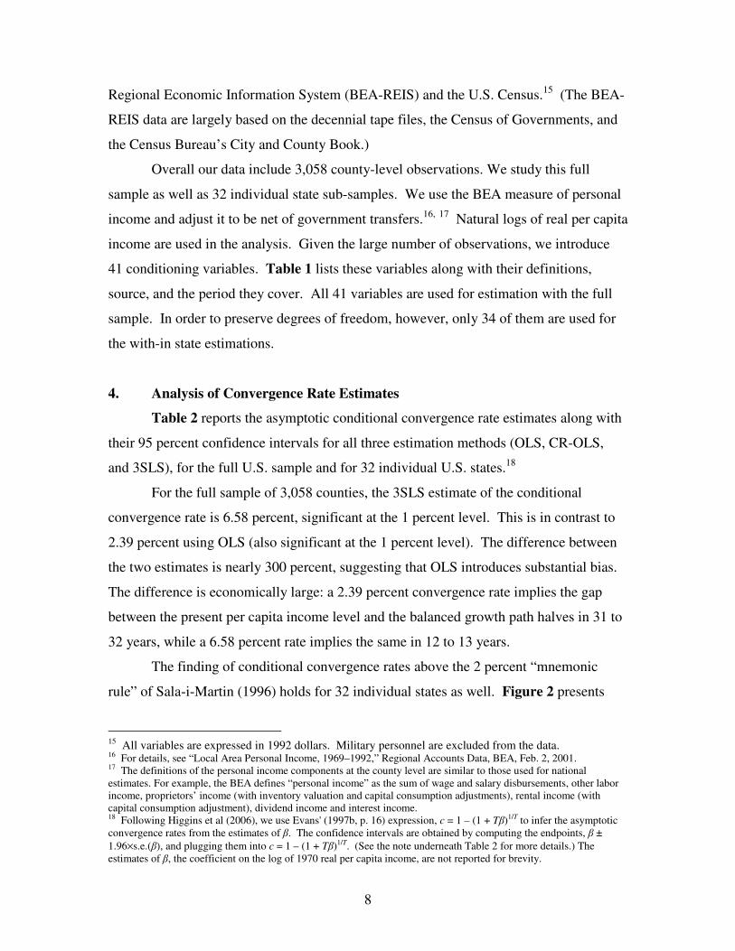
Regional Economic Information System (BEA-REIS) and the U.S. Census.15

(The BEA-

REIS data are largely based on the decennial tape files, the Census of Governments, and

the Census Bureau’s City and County Book.)

Overall our data include 3,058 county-level observations. We study this full

sample as well as 32 individual state sub-samples. We use the BEA measure of personal

income and adjust it to be net of government transfers.16,

17

Natural logs of real per capita

income are used in the analysis. Given the large number of observations, we introduce

41 conditioning variables. Table 1 lists these variables along with their definitions,

source, and the period they cover. All 41 variables are used for estimation with the full

sample. In order to preserve degrees of freedom, however, only 34 of them are used for

the with-in state estimations.

4. Analysis of Convergence Rate Estimates

Table 2 reports the asymptotic conditional convergence rate estimates along with

their 95 percent confidence intervals for all three estimation methods (OLS, CR-OLS,

and 3SLS), for the full U.S. sample and for 32 individual U.S. states.18

For the full sample of 3,058 counties, the 3SLS estimate of the conditional

convergence rate is 6.58 percent, significant at the 1 percent level. This is in contrast to

2.39 percent using OLS (also significant at the 1 percent level). The difference between

the two estimates is nearly 300 percent, suggesting that OLS introduces substantial bias.

The difference is economically large: a 2.39 percent convergence rate implies the gap

between the present per capita income level and the balanced growth path halves in 31 to

32 years, while a 6.58 percent rate implies the same in 12 to 13 years.

The finding of conditional convergence rates above the 2 percent “mnemonic

rule” of Sala-i-Martin (1996) holds for 32 individual states as well. Figure 2 presents

15

All variables are expressed in 1992 dollars. Military personnel are excluded from the data. 16 For details, see “Local Area Personal Income, 1969–1992,” Regional Accounts Data, BEA, Feb. 2, 2001. 17 The definitions of the personal income components at the county level are similar to those used for national

estimates. For example, the BEA defines “personal income” as the sum of wage and salary disbursements, other labor

income, proprietors’ income (with inventory valuation and capital consumption adjustments), rental income (with

capital consumption adjustment), dividend income and interest income. 18 Following Higgins et al (2006), we use Evans' (1997b, p. 16) expression, c = 1 – (1 + Tβ)1/T to infer the asymptotic

convergence rates from the estimates of β. The confidence intervals are obtained by computing the endpoints, β ±

1.96×s.e.(β), and plugging them into c = 1 – (1 + Tβ)1/T. (See the note underneath Table 2 for more details.) The

estimates of β, the coefficient on the log of 1970 real per capita income, are not reported for brevity.

9

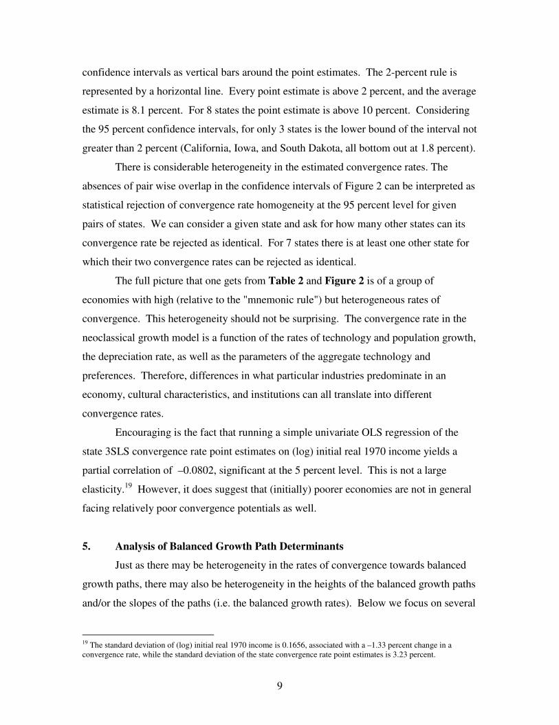
confidence intervals as vertical bars around the point estimates. The 2-percent rule is

represented by a horizontal line. Every point estimate is above 2 percent, and the average

estimate is 8.1 percent. For 8 states the point estimate is above 10 percent. Considering

the 95 percent confidence intervals, for only 3 states is the lower bound of the interval not

greater than 2 percent (California, Iowa, and South Dakota, all bottom out at 1.8 percent).

There is considerable heterogeneity in the estimated convergence rates. The

absences of pair wise overlap in the confidence intervals of Figure 2 can be interpreted as

statistical rejection of convergence rate homogeneity at the 95 percent level for given

pairs of states. We can consider a given state and ask for how many other states can its

convergence rate be rejected as identical. For 7 states there is at least one other state for

which their two convergence rates can be rejected as identical.

The full picture that one gets from Table 2 and Figure 2 is of a group of

economies with high (relative to the "mnemonic rule") but heterogeneous rates of

convergence. This heterogeneity should not be surprising. The convergence rate in the

neoclassical growth model is a function of the rates of technology and population growth,

the depreciation rate, as well as the parameters of the aggregate technology and

preferences. Therefore, differences in what particular industries predominate in an

economy, cultural characteristics, and institutions can all translate into different

convergence rates.

Encouraging is the fact that running a simple univariate OLS regression of the

state 3SLS convergence rate point estimates on (log) initial real 1970 income yields a

partial correlation of –0.0802, significant at the 5 percent level. This is not a large

elasticity.19

However, it does suggest that (initially) poorer economies are not in general

facing relatively poor convergence potentials as well.

5. Analysis of Balanced Growth Path Determinants

Just as there may be heterogeneity in the rates of convergence towards balanced

growth paths, there may also be heterogeneity in the heights of the balanced growth paths

and/or the slopes of the paths (i.e. the balanced growth rates). Below we focus on several

19 The standard deviation of (log) initial real 1970 income is 0.1656, associated with a –1.33 percent change in a

convergence rate, while the standard deviation of the state convergence rate point estimates is 3.23 percent.

10

conditioning variables. In our regressions, their coefficients indicate their effects on the

average growth rate of per capita income indirectly via the height of the balanced growth

paths. Given that height, the average growth rate increases (if higher) or decreases (if

lower) as a result of the distance of per capita income from the balanced growth path and

the convergence effect towards that path.20

The variables we focus on are grouped into public sector size variables,

educational attainment variables, and industry composition variables. In each case we

focus on 3SLS estimates. We discuss the results for the entire sample, and to address

potential cross-state heterogeneity, for individual states as well.

i. Size of the Public Sector

Does government foster or hinder economic growth? A large literature explores

this question in a cross-section of countries.21

These studies use government expenditure

variables to capture the size and scope of government. We, in contrast, use the percent of

a county’s population employed by the federal, state and local governments, which offer

certain advantages over expenditure variables. First, the three separate measures allow us

to explore how the link between the public sector and growth varies at three levels of

decentralization. Second, the separate measures can help to alleviate problems of

interpreting coefficients when externalities exist. For example, the local government

variable should be nearly immune to spill-over effects.

Our employment variables complement the expenditure variables used in previous

studies because employment variables can be interpreted as a stock of government

activities producing a flow of services, while government expenditures are the flow of

services. While previous studies directly account for government expenditure, our

employment variables directly account for the extent to which government is involved in

20 If conditional convergence were to be rejected, then these coefficients might be interpreted as influences on

economies’ balanced growth rates. However, since we report results only for states where 3SLS convergence rates

were statistically significant, conditioning variable coefficient estimates can be interpreted as effects on the height of

balanced growth paths throughout this paper. 21 Barro (1991) and Folster and Henrekson (2001) find that a large public sector is growth hindering. Easterly and

Rebelo (1993) find that public investments in transportation and communication accelerate economic growth, but that

links between growth and other fiscal variables are fragile. Evans and Karras (1994) report that government activities,

except education services, are either unproductive or affect growth negatively in a cross-section of the U.S states.

11

the economy, i.e. the percent of labor force activities directed by government.22

Also,

whereas expenditure measures can provide useful differentiation of roles of government,

our variables provide another differentiation of roles, those associated with federal

government versus those of state and local governments.

Table 3 summarizes the results. In the full sample, we find a negative and

statistically significant relationship between the percent of the population employed by

government and the growth rate. Furthermore, the negative effect does not diminishing

at more decentralized levels. The coefficients for the federal, state and local variables are

–0.0226, –0.0163, and –0.0204 respectively (all significant at the 1 percent level).23

Considering the individual states, we see that in vast majority of the cases, there is

no statistically significant relationship between the three government employment

variables and growth. Federal government employment coefficient is statistically

significant in four states, the state government in five states, and the local government in

six states. Of these 15 statistically significant coefficient estimates, 11 are negative and

four positive. The positive coefficients are obtained in North Dakota (for all three

government employment variables) and in Kansas (for the local government variable).

For all three variables we find some heterogeneity. Focusing on cases with

negative coefficients, the statistically significant federal, state, and local government

estimates range from –0.0917 (Missouri) to –0.1368 (Idaho), from –0.0422 (North

Carolina) to –0.0729 (Colorado), and from –0.0431 (Minnesota) to –0.1792 (Louisiana),

respectively.

In sum, we find a negative relationship between the size of government and the

rate of economic growth when we consider the entire U.S. For 30 of the 32 individual

states analyzed here, government at all levels of decentralization has either no

statistically-discernable effects, or worse yet, has negative effects, which is similar to the

findings reported by Evans and Karras (1994). As such, discernable differences between

22 Obviously, expenditure and involvement are not mutually exclusive. Government expends wages so that labor is

involved in government activities. As well, government expenditures are part of market demand and, therefore,

influence the allocation of resources in the private sector. 23 Besides the public sector hindering economic growth via distortions of incentives and diversion of resources, another

possibility is that non-government wage growth simply outpaces government wage growth. We looked at wage data

for the 1970-1998 period. At the state and federal level, government wage growth outpaced non-government wage

growth in approximately 45 percent of counties. At the local level, government wages grew faster in over 70 percent of

counties. These differences do not appear strong enough to drive the federal and state estimates, and would work

against the local estimates.

12

“good” versus “bad” governments across states cannot be detected (the possible

exception being North Dakota with its positive and significant coefficients for each level

of government employment).

ii. Educational Attainment

Our data include 8 measures of educational attainments. We focus on four: the

percent of the population with (a) 9 to11 years of education, (b) high school diploma, (c)

some college education, and (d) bachelor degree or more. Table 4 reports the 3SLS

coefficient estimates for these variables.

Consider the percent of the population with at least 9 years of education, but less

than a high school degree. For the full sample the coefficient is –0.0204, significant at

the 1 percent level. This seems sensible, implying that the greater percentage of

population without the skills necessary to obtain a high school diploma, the lower the

balanced growth path. Passing that threshold, the coefficient for the population achieving

a high school diploma has an estimate of 0.0091, also significant at the 1 percent level.

More surprisingly, the coefficient for the percent of the population with some

college education is negative and insignificant. Compare this to the coefficient on the

percent of the population with a bachelor degree or more: 0.0701, significant at the 1

percent level. A possible interpretation of this result concerns the opportunity cost of

education: college education increases individual skills but it is costly (foregone wages).

The results may imply that a complete college education represents a positive net return

to individuals, while the net return on a 2-year degree is questionable. Kane and Rouse

(1995) and Surette (1997) report that the estimated return to 2-year degrees is positive

and equals about 4-6 percent and 7-10 percent, respectively. Neither of these studies uses

county-level data, however. In addition, these studies do not take into account the social

return, which our results presumably do. Both studies look at costs (tuition, wages

forgone, experience forgone, etc.) and benefits (wage premiums) while we consider the

effect of educational attainment on the average growth of an economy over a 30-year

period. What we might be detecting in our results, therefore, is a questionable social

return to associate degrees. This is a potentially important finding for policy-makers

because, as Kane and Rouse (1995, p.600n) note, “Twenty percent of Federal Pell Grants,

13

10 percent of Guaranteed Student Loans, and over 20 percent of state expenditures for

postsecondary education, go to community colleges.”

In all four categories we can detect some heterogeneity across states. For the “9

to 11 years” variable, there are 6 statistically significant coefficient estimates, ranging

from –0.0544 (Texas) to 0.1323 (Colorado). A possible explanation for the positive

coefficients may concern compulsory education laws. The variable may include students

who would not have pursued a high school education given their druthers but were forced

to. There is an opportunity cost forced on rather-be-truant individuals and also a direct

cost on school system to deal with them. If individuals are pushed through the school

system while not receiving the benefits of education, they forego the productive

opportunities available and absorb resources that could have been spent on willing

students. The data, however, is silent on this as each of the 6 states has roughly similar

age spans of compulsion.

Some heterogeneity is also detected across the “high school diploma” variable

coefficients. Of the 6 statistically significant coefficients, one is negative (Mississippi),

while the remaining five are positive ranging from 0.0474 (Kentucky) to 0.1085

(Idaho).24

For the some college education variable, the statistically significant coefficient

estimates are all positive and range from 0.0390 (Texas) to 0.1493 (North Dakota).

Finally, for the bachelor degree or more variable, we have 11 statistically significant

coefficients, all positive, ranging from 0.0743 (Ohio) to 0.1764 (Tennessee).

In sum, of the four educational attainment variables, the “bachelor degree or

more” variable appears to be the most robust and economically the most important.

iii. Industry Composition Effects

Our data include 16 industry-level variables, measuring the percent of the

population employed in the given industry. Here we focus on three industry categories

that have significant estimated effects for the full sample: (a) finance, insurance and real

24 A reasonable explanation for this heterogeneity might be that schools are better in some states than others. This can

be informally tested by comparing average scholastic aptitude test (SAT) scores from the states with negative

coefficient estimates to those with positive coefficient estimates. It turns out however, that Mississippi has SAT

average scores neither exceptionally high nor low relative to the other five states. This argument assumes that the

predominant portion of the population with high school degrees obtained their diplomas in the considered state. For

entire states, this seems a priori plausible but not certain.

14

estate, (b) educational services, and (c) entertainment and recreational services. The

coefficients estimates for these variables are summarized in Table 5.

a. Finance, Insurance and Real Estate Services

We find positive correlation between the percent of the population employed in

finance, insurance and real estate services and economic growth in the full sample. The

coefficient estimate is 0.0731, significant at the 1 percent level. This might be a

reflection of the link between financial intermediation and economic growth. Rousseau

and Wachtel (1998) report similar findings and Greenwood and Jovanovic (1990) and

King and Levine (1993) offer theoretical models predicting this link.

We find qualitative, as well as quantitative, heterogeneity across individual states.

For 6 states, coefficient estimates are statistically significant. For Louisiana the estimate

is negative, for which we have no explanation. For five states, the coefficient estimate is

positive, ranging from 0.1292 (Illinois) to 0.6835 (North Dakota).

b. Educational Services

The percent of the population providing education services is negatively

correlated with growth in the full sample, with a point estimate of –0.0445, but it is not

significant statistically. For individual states, we find six cases of statistically significant

coefficients, all negative, ranging from –0.1407 (Illinois) to –0.4666.

A possible reason for the negative relation might be that the benefits of education

provided in a county are not entirely internalized by the county itself. We find a positive

correlation between some measures of human capital stocks and growth in section 5.ii,

but the correlation is silent as to where the stocks are accumulated. For example,

students may attend a college in one county but then move to another county as they join

the workforce.25

Higgins et al (2006) report that this negative association is particularly

strong in metro counties. This is consistent with an externality argument in that a large

25 Another explanation could be a bureaucratic over-expansion of the public school systems. This is explored by

Marlow (2001) for California districts, and finds that an increase in the number of teachers has no statistically

significant effect on SAT scores or dropout rates, while an increase in the size of administrative staff increases the SAT

scores and decreases dropout rates.

15

proportion of colleges and universities are in metro areas, but many students leave the

metro areas upon graduation.

c. Entertainment and Recreational Services

The estimated effect of the percent of the population employed in entertainment

and recreation industries is positive and significant in the full sample with the point

estimate of 0.0166. This effect is important because entertainment and recreation

services comprise an increasingly large segment of the U.S. economy (Costa, 1997).

Seven states have statistically significant coefficients, and all seven are positive,

ranging from 0.1751 (California) to 0.9807 (Mississippi).26

This positive correlation

might be capturing the attraction of economic activity to counties with gambling casinos

and professional sport teams (NHL, MLB, NFL, and NBA), as reported by Walker and

Jackson (1998), Eadington (1999), and Siegfried and Zimbalist (2000).

6. Model Uncertainty

Growth theories are silent as to which independent variables belong in growth

regressions. In response to these sensitivity issues, Leamer (1983, 1985) proposes an

extreme bound analysis to identify “robust” empirical relations. For a specific variable of

interest, the extreme bounds of the distribution of the associated coefficient estimate are

calculated as a range from the smallest to the largest value the coefficient can take given

all possible combinations of the remaining independent variables taken 3 at a time. If the

two bounds have differing signs, then the variable is labeled as fragile.

Levine and Renelt (1992), employing a version of Leamer’s extreme bound

analysis, show that cross-country regression results are sensitive to small changes in the

set of conditioning variables. In fact they show that very few variables are robustly

related to growth. More recently, Sala-i-Martin et al. (2004) introduce an alternative

method, Bayesian Averaging of Classical Estimates (BACE), to test the robustness of 67

independent variables. They find 18 variables significantly and robustly partially

correlated with long term economic growth, with one of the stronger findings relating to

26 The finding that California has the lowest point estimate is counter to what “common belief” would suggest that the

home of Hollywood would be one where entertainment industry fostered economic growth.

16

the initial level of real GDP per capita.

In order to determine whether any of our results are model dependent, we

replicate Levine and Renelt’s implementation of Leamer’s extreme bound analysis on our

main variables of interest for the full sample: initial level of real per capita income;

federal government employment; state government employment; local government

employment; 9-11 years of education; high school diploma; some college education;

bachelor degree or higher; finance, insurance and real estate; educational services; and,

entertainment and recreational services.27

It should be noted that while Sala-i-Martin et

al. (2004) consider 67 independent variables, very few of them overlap with our 41

independent variables. The same applies for the variables considered by Levine and

Renelt (1992). The main reason for this is the level of analysis; we are focusing on

county-level variables whereas they are focusing on national/international-level variables.

Of the 11 variables for which we conduct an extreme bound analysis, all of them

except state government employment, high school diploma, some college education, and

educational services are robustly related to economic growth. The two extreme bounds

for these other four variables (state government employment, high school diploma, some

college education and educational services), while significant at least at the 5 percent

level, have opposite signs which suggests these variables are “fragile”.

Overall our results differ from the previous work studying the robustness of

empirical findings. Unlike Levine and Renelt (1992) who find very few variables

robustly related to growth, the majority of our variables our robustly related. This could

be because the variables available at the county-level for the U.S. are, in principle, better

indicators of growth determinants than the variables available for cross-country samples.

Alternatively, the quality and comparability of data across counties may make our

variables more effective at capturing growth effects in practice. While making inferences

about international growth experiences from the data of a single country is perilous, the

robustness of our results suggests that results from county-level data may be able to make

contributions to understanding more than just the U.S. experience.

27

Levine and Renelt’s implementation of Leamer’s methodology is available in Stata 9.0 using the “eba”

command.

17

7. Conclusions

We use over 3,000 U.S. county-level data on 41 socio-economic variables to

explore the variation in growth determination and income convergence across the U.S.

states. We employ a consistent 3SLS estimation procedure that does not bias

convergence rate estimates downward.

Convergence across the U.S. averages nearly 7 percent per year—higher than the

2 percent normally found with OLS. Across 32 individual states, estimated convergence

rates are above 2 percent with an average of 8.1 percent. For 30 states the convergence

rate is above 2 percent with 95 percent confidence. We find substantial heterogeneity in

individual state convergence rates. For 7 states the convergence rate can be rejected as

identical to at least one other state’s convergence rate with 95 percent confidence.

The high convergence rates are encouraging in the sense that, given proper

policies to induce and support balanced growth paths, laggard economies can close the

gap relatively quickly. Also encouraging is the fact that the partial correlation between

convergence rates and initial income is negative. However, when one considers the

heterogeneity in convergence rate estimates across U.S. states, one suspects that the

heterogeneity in convergence rates across countries is likely more pronounced. Since

most cross-country empirical studies estimate a single convergence rate, the possibility of

individual laggard economies with poor convergence prospects cannot be ruled out.

In examining the determinants of balanced growth path heights, we find that

government at all levels of decentralization is either unproductive or perhaps even worse,

is negatively correlated with economic growth. Educational attainment of a population

has a non-linear relationship with economic growth: growth is positively related to high-

school degree attainment, unrelated to obtaining some college education, and then

positively related to four-year or more degree attainment. Also, finance, insurance and

real estate industry and entertainment industry are positively correlated with growth,

while education industry is negatively correlated with growth. However, heterogeneity in

the effects of balanced growth path determinants across individual states is harder to

detect than heterogeneity of convergence rates.

We should note that our convergence rate estimates are ultimately, based on a

specification from the neoclassical growth model. That model is of a closed economy

18

and convergence is a phenomenon based entirely on diminishing returns to accumulated

capital—specifically capital accumulated from the economy’s own savings.28

However,

across U.S. counties, especially within a given state, there is considerable capital

mobility. Perfect capital mobility would predict immediate equalization of returns and

instantaneous convergence, but convergence rates less than 100 percent may still obtain

for open economies in the presence of adjustment costs to capital as well as imperfect

capital markets (Levy, 2000 and 2004). Barro et al. (1995) demonstrate that gradual

convergence will occur under partial capital mobility because “borrowing is possible to

finance accumulation of physical capital, but not accumulation of human capital” (p.

104). If human capital accounts for a large share of income (Barro and Sala-i-Martin,

1992, and Mankiw et al, 1992 suggest about one half), that can lead to gradual

convergence.29

These assumptions would imply (gradual) conditional convergence, and represent

factors that would place reality somewhere between the convergence rate of a closed

economy and the instant convergence of an open economy with perfect capital markets.

Our estimates represent the effective convergence rates associated with that reality, or

those realities specific to given states and, as such, an additional source of heterogeneity.

Some readers have questioned the applicability of the neoclassical growth model

to the U.S. counties. We agree that the model may not be the most suitable framework

for thinking about growth in U.S. counties given their extraordinary degree of openness.

Rappaport (1999, 2004, 2005, and 2006) proposes a way around this problem by offering

a version of the model for studying local growth, where by “local” is meant small open

economic units comprising a larger entity, such as counties comprising the U.S. The

distinguishing characteristic of small open economies such as U.S. counties is the

extraordinary mobility of labor. The question, then, is how does labor mobility affect

convergence? Rappaport (1999, 2005) expands the model by allowing labor mobility and

28 This can include both physical and, in the case of the augmented Solow model (Mankiw et al, 1992), human capital. 29 At the state level, there is evidence that even financing of physical capital from one state to another is not perfect.

Driscoll (2004) finds that state-specific variation in deposits has a large effect on state-specific loans. The intuition is

that some firms that do not regard bank loans and forms of direct finance as perfect substitutes and out-of-state bank

lending is not prevalent. U.S. Federal regulation, until recently, restricted out-of-state bank lending and, even as late as

1994, more than 70 percent of bank assets were in the control of within-state entities (Berger et al, 1995).

19

finds that the model predicts conditional convergence, which is what we find here.30

Future research could explore interactions of initial income and educational

attainment in a more systematic way. Further, questions of the type explored here could

be addressed using similar kind of county or district level data from other countries.

30 Further, Rappaport (1999, 2005) finds that that convergence can either be accelerated (by a positive effect of out-

migration on wages) or slowed (by a resultant disincentive for capital accumulation) depending on relative changes in

marginal products. Rappaport's (2005) analysis suggests that at low levels of income the later effect dominates.

20

Data Appendix: Measurement of Per Capita Income

Because of the critical importance of the income variable for the study of growth

and convergence, we want to address its measurement in some detail. Two options were

available to us for the construction of the county-level per capita income variable: (1)

Census Bureau database, and (2) BEA-REIS database.

Income information collected by the Census Bureau for states and counties is

prepared decennially from the “long-form” sample conducted as part of the overall

population census (BEA, 1994). This money income information is based on the self-

reported values by Census Survey respondents. An advantage of the Census Bureau’s

data is that they are reported and recorded by place of residence. These data, however, are

available only for the “benchmark” years, i.e., the years in which the decennial Census

survey is conducted.

The second source for this data, and the one chosen for this project, is personal

income as measured by the Bureau of Economic Analysis (BEA).1 The definitions that

are used for the components of personal income for the county estimates are essentially

the same as those used for the national estimates. For example, the BEA defines

“personal income” as the sum of wage and salary disbursements, other labor income,

proprietors’ income (with inventory valuation and capital consumption adjustments),

rental income (with capital consumption adjustment), personal dividend income and

personal interest income. (BEA, 1994) “Wage and salary disbursements’ are

measurements of pre-tax income paid to employees. “Other labor income” consists of

payments by employers to employee benefit plans. “Proprietors’ income” is divided into

two separate components—farm and non-farm. Per capita income is defined as the ratio

of this personal income measure to the population of an area.

The BEA’s estimates of personal income reflect the revised national estimates of

personal income that resulted from the 1991 comprehensive revision and the 1992 and

1993 annual revisions of the national income and product accounts. The revised national

estimates were incorporated into the local area estimates of personal income as part of a

comprehensive revision in May 1993. In addition, the estimates incorporate source data

1 The data and their measurement methods are described in detail in “Local Area Personal Income, 1969–1992” published by the BEA under the Regional Accounts Data, February 2, 2001.

21

that were not available in time to be used in the comprehensive revisions.2

The BEA compiles data from several different sources in order to derive this

personal income measure. Some of the data used to prepare the components of personal

income are reported and recorded by place of work rather than place of residence.

Therefore, the initial estimates of these components are on a place-of-work basis.

Consequently, these initial place-of-work estimates are adjusted so that they will be on a

place-of-residence basis and so that the income of the recipients whose place of residence

differs from their place of work will be correctly assigned to their county of residence.

As a result, a place of residence adjustment is made to the data. This adjustment is

made for inter-county commuters and border workers utilizing journey-to-work (JTW)

data collected by Census. For the county estimates, the income of individuals who

commute between counties is important in every multi-county metropolitan area and in

many non-metropolitan areas. The residence adjustment estimate for a county is

calculated as the total inflows of the income subject to adjustment to county i from

county j minus the total outflows of the income subject to adjustment from county i to

county j. The estimates of the inflow and outflow data are prepared at the Standard

Industrial Classification (SIC) level and are calculated from the JTW data on the number

of wage and salary workers and on their average wages by county of work for each

county of residence from the Population Census.

Given the data constraints, it was necessary to use an interpolation procedure for

some variables.3 In this study we cover the 1970–1998 period. However, in order to

implement the Evans’ (1997a, 1997b) 3SLS estimation method as described in section 2,

we needed to have available data values for 1969 and 1997. We used a linear

interpolation method to generate these missing observations. It should be noted that none

of the data relating to income and population variables were generated by this method, as

they were available from BEA-REIS on a yearly basis for the entire period covered. The

Census data variables, which were available in 1970, 1980 and 1990, were interpolated in

order to generate the 1969, 1997, and 1998 values.

2 For details of these revisions, see “Local Area Personal Income: Estimates for 1990–92 and Revisions to the Estimates for 1981–91,” Survey of Current Business 74 (April 1994), 127–129. 3 Given the cross-section nature of our data, the use of interpolation does not cause problems of the type reported by Dezhbakhsh and Levy (1994) in their study of periodic properties of interpolated time series.

22

References

Agrawal, Ajay, Ian Cockburn (2003), “The Anchor Tenant Hypothesis: Exploring the Role of Large, Local, R&D Intensive Firms in Regional Innovation Systems,” International Journal of Industrial Organization 21, 1227–1253.

Barkley, David (1988), “The Decentralization of High-Technology Manufacturing to Nonmetropolitan

Areas,” Growth and Change, 13–30. Barkley, David, Mark Henry, Dohee Lee (2006), “Innovative Activity in Rural Areas,” Unpublished

working paper, Clemson University, Department of Applied Economics and Statistics. Barro, Robert J. (1991), “Economic Growth in a Cross Section of Countries,” Quarterly Journal of

Economics 106, 407–443. Barro, Robert J. (1997), Determinants of Economic Growth: A Cross-Country Empirical Study

(Cambridge, MA: MIT Press). Barro, Robert J., Mankiw, N. Gregory and Sala-Martin, Xavier (1995), “Capital Mobility in Neoclassical

Models of Growth,” American Economic Review 85, 103–115. Barro, Robert J. and Sala-I-Martin, Xavier (1991), “Convergence across States and Regions,” Brookings

Papers on Economic Activity 1, 107–158. Barro, Robert J. and Sala-i-Martin, Xavier (1992), “Convergence,” Journal of Political Economy 100,

223–251. Berger, A.N., Kashyap, Anil K. and Hannan, T.H. (1995), “The Transformation of the U.S. Banking

Industry: What a Long, Strange Trip It’s Been,” Brookings Papers on Economic Activity 2, 55–218.

Bliss, Christopher (1999), “Galton’s Fallacy and Economic Convergence,” Oxford Economic Papers 51,

4–14. Brock, William A. and Steven N. Durlauf (2001), “Growth Empirics and Reality,” World Bank Economic

Review 15, 229–272. Canova, Fabio (2004), “Testing for Convergence Clubs in Income Per Capita: A Predictive Density

Approach,” International Economic Review 45, 49–77. Caselli, Francesco, Esquivel, Gerardo and Lefort, Fernando (1996), “Reopening the Convergence Debate:

A New Look at Cross-Country Growth Empirics,” Journal of Economic Growth 1, 363–389. Colorado Department of Education, “Title 22, Colorado Revised Statutes: Education Article 33: School

Attendance Law of 1963 Section 104.” Conley, Timothy J. (1999), “GMM Estimation with Cross Sectional Dependence,” Journal of

Econometrics 92, 1–45. Cooke, Phillip (2002), “Regional Innovation Systems: General Findings and Some Evidence from

Biotechnology Clusters,” Journal of Technology Transfer 27, 133–145. Costa, Dora L. (1997), “Less of a Luxury: The Rise of Recreation since 1888,” NBER Working Paper No.

6054, June.

23

Desdoigts, Alan (1999), “Patterns of Economic Development and the Formation of Clubs,” Journal of Economic Growth 4, 305–330.

Dezhbakhsh, Hashem and Daniel Levy (1994), “Periodic Properties of Interpolated Time Series,”

Economics Letters 44, 221–228. Driscoll, John C. (2004), “Does Bank Lending Affect Output? Evidence from the U.S. States,” Journal of

Monetary Economics 51, 451–471. Durlauf, Steven N. and Paul A. Johnson (1995), “Multiple Regimes and Cross-Country Growth Behavior,”

Journal of Applied Econometrics 10, 365–384. Durlauf, Steven N., Andros Kourtellos, and Artur Minkin (2001), “The Local Solow Growth Model,”

European Economic Review 45, 928–940. Eadington, William R. (1999). “The Economics of Casino Gambling,” Journal of Economic Perspectives

13, 173–192. Easterly, William and Sergio Rebelo (1993), “Fiscal Policy and Economic Growth,” Journal of Monetary

Economics 32, 417–458. Evans, Paul (1997a), “How Fast Do Economies Converge?” Review of Economics and Statistics 36, 219–

225. Evans, Paul (1997b), “Consistent Estimation of Growth Regressions,” unpublished manuscript, available at

http://economics.sbs.ohiostate.edu/pevans/pevans.html. Evans, Paul (1998), “Using Panel Data to Evaluate Growth Theories,” International Economics Review

39, 295–306. Evans, Paul and Georgios Karras (1994), “Are Government Activities Productive? Evidence from a Panel of

U.S. States” Review of Economics and Statistics 76, 1–11. Folster, Stefan and M. Henrekson (2001), “Growth Effects of Government Expenditure and Taxation in

Rich Countries,” European Economic Review 45, 1501–1520. Greenwood, Jeremy and Boyan Jovanovic (1990), “Financial Development, Growth, and the Distribution

of Income,” Journal of Political Economy 98, 1076–1107. Higgins, Matthew, Daniel Levy and Andrew T. Young (2006), “Growth and Convergence across the U.S:

Evidence from County-Level Data,” Review of Economics and Statistics 88(4), 671–681. Higgins, Matthew, Andrew T. Young, Daniel Levy (2009), “Federal, State and Local Governments:

Evaluating their Separate Roles in US Growth,” Public Choice 139, 493–507. Islam, Nazrul (1995), “Growth Empirics: A Panel Data Approach,” Quarterly Journal of Economics 110,

1127–1170. Jaffe, Adam, Manuel Trajtenberg, Rebecca Henderson (1993), “Geographic Localization of Knowledge

Spillovers as Evidenced by Patent Citations,” The Quarterly Journal of Economics 108(3), 577–598.

Kane, Thomas J. and Cecilia E. Rouse (1995), “Labor-Market Returns to Two- and Four-Year College,”

American Economic Review 85, 600–614.

24

King, Robert G. and Ross Levine (1993), “Finance and Growth: Schumpeter May be Right,” Quarterly Journal of Economics 108, 717–737.

Leamer, Edward (1983), “Let’s Take the Con out of Econometrics,” American Economic Review 73(1),

31–43. Leamer, Edward (1985), “Sensitivity Analysis Would Help,” American Economic Review 75(3), 308–313. Lee, Kevin, M. Hashem Pesaran and Ron Smith (1997), “Growth and Convergence in a Multi-Country

Empirical Stochastic Growth Model,” Journal of Applied Econometrics 12, 357–384. Levine, Ross and D. Renelt (1992), “A Sensitivity Analysis of Cross-Country Growth Regressions,”

American Economic Review 82, 942–963. Levy, Daniel (2000), “Investment-Saving Co-Movement and Capital Mobility: Evidence from Century

Long U.S. Time Series” Review of Economic Dynamics 3, 100–136. Levy, Daniel (2004), “Is the Feldstein-Horioka Puzzle Really a Puzzle?” in Aspects of Globalization:

Macroeconomic and Capital Market Linkages in the Integrated World Economy, edited by Christopher Tsoukis, George M. Agiomirgianankis, and Tapan Biswas (London: Kluwer Academic Publishers), 49–66.

Levy, Daniel and H. Dezhbakhsh (2003), “International Evidence on Output Fluctuation and Shock

Persistence,” Journal of Monetary Economics 50, 1499–1530. Mankiw, N. Gregory, David Romer, and David N. Weil (1992), “A Contribution to the Empirics of

Economic Growth,” Quarterly Journal of Economics 107, 407–437. Marlow, Michael L. (2001), “Bureaucracy and Student Performance in U.S. Public Schools,” Applied

Econometrics 33, 1314–1350. Quah, Danny T. (1996), “Twin Peaks: Growth and Convergence in Models of Distributional Dynamics,”

Economic Journal 106, 1045–1055. Quah, Danny T. (1997), “Empirics for Growth and Distribution: Stratification, Polarization, and

Convergence Clubs,” Journal of Economic Growth 2, 27–59. Rappaport, Jordan (1999), “Local Growth Empirics,” CID W.P. #23, Harvard University. Rappaport, Jordan (2000), “Is the Speed of Convergence Constant?” Working Paper No. 00-10, Federal

Reserve Bank of Kansas City. Rappaport, Jordan (2004), “Why Are Population Flows so Persistent?” Journal of Urban Economics 56,

554–580. Rappaport, Jordan (2005), “How Does Labor Mobility Affect Income Convergence?” Journal of

Economic Dynamics and Control 29, 567–581. Rappaport, Jordan (2006), “Moving to Nice Weather,” Regional Science and Urban Economics,

forthcoming. Rappaport, Jordan and Jeffrey D. Sachs (2003), “The United States as a Coastal Nation,” Journal of

Economic Growth 8, 5–46.

25

Rousseau, Peter L. and Paul Wachtel (1998), “Financial Intermediation and Economic Performance: Historical Evidence from Five Industrialized Countries,” Journal of Money, Credit and Banking 30, 657–678.

Sala-i-Martin, Xavier X. (1996), “Regional Cohesion: Evidence and Theories of Regional Growth and

Convergence,” European Economic Review 40, 1325–1352. Sala-i-Martin, Xavier, Gernot Doppelhofer, Ronald Miller (2004), “Determinants of Long-Term Growth: A

Bayesian Averaging of Classical Estimates (BACE) Approach,” American Economic Review 94(4), 813–835.

Shaffer, Sherrill (2006), “Establishment Size by Sector and County-Level Economic Growth,” Small

Business Economics 26, 145–154. Siegfried, John and Andrew Zimbalist (2000), “The Economics of Sports Facilities and Their

Communities,” Journal of Economic Perspectives 14, 95–114. Surette, Brian J. (1997), “The Effects of Two-Year College on the Labor Market and Schooling

Experiences of Young Men,” Board of the Governors of the Federal Reserve System, Finance and Economic Discussion Series, No. 1997/44.

U.S. Department of Education (1999–2000), National Center for Education Statistics, Schools and Staffing

Survey, 1999–2000. Tables 1.01 and 2.01. U.S. Department of Education (2001), Digest of Education Statistics, Table 151. U.S. Department of Education (2001), Digest of Education Statistics, Table 137. Walker, Douglas M. and John D. Jackson (1998), “New Goods and Economic Growth,” Review of

Regional Studies 28, 47–69 Young, Andrew T., Matthew J. Higgins, Daniel Levy (2008), “Sigma Convergence vs. Beta Convergence:

Evidence from U.S. County-Level Data,” Journal of Money, Credit and Banking 40, 1083–1093. Zucker, Lynne, Michael Darby, Marilynn Brewer (1998), “Intellectual Human Capital and the Birth of US

Biotechnology Enterprises,” American Economic Review 88(1), 290–306.

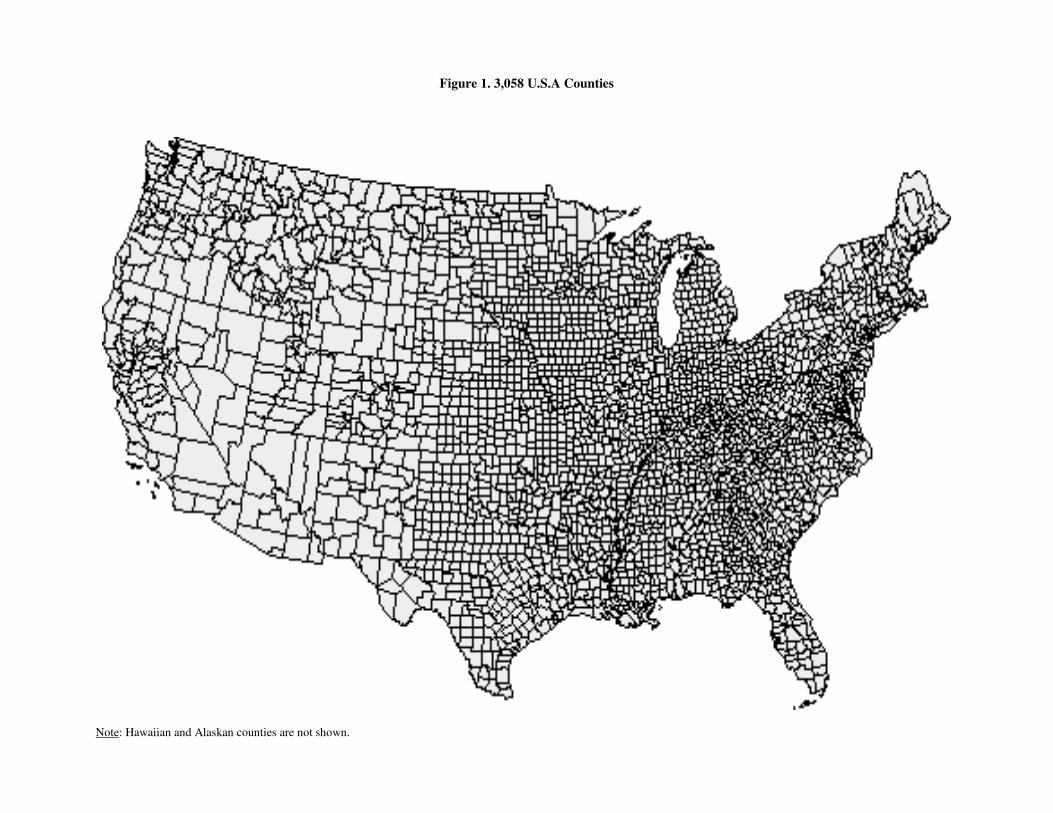
Figure 1. 3,058 U.S.A Counties

Note: Hawaiian and Alaskan counties are not shown.

Figure 2. Point Estimates of Within-State Asymptotic Convergence Rates with 95% Confidence

Intervals

0.00

0.05

0.10

0.15

0.20

Alaba

ma

Arkan

sas

Cal

iforn

iaC

olor

ado

Flor

ida

Geo

rgia

Idah

oIll

inoi

sIn

dian

aIo

wa

Kansa

sKen

tuck

yLo

uisia

naM

ichi

gan

Min

neso

taM

issis

sipp

iM

isso

uri

Mon

tana

New

Yor

k

Nor

th C

arol

ina

Nor

th D

akot

aO

hio

Okl

ahom

a

Penns

ylva

nia

South

Car

olin

a

South

Dak

ota

Tenn

esse

eTe

xas

Virgin

ia

Was

hing

ton

Wes

t Virg

inia

Wis

onsi

n

Lower Point Upper

0.02

Table 1. Variable Definitions

Variable Definition Period Source

Income Per Capita Personal Income (excluding transfer

payments)

1969–1998 BEA

Land area per capita Land area in km2/population 1970-1990 Census

Water area per capita Water area in km2/population 1970-1990 Census

Age: 5-13 years Percent of 5–13 year olds in the population 1970-1990 Census



Age: 65+ Percent of 65+ olds 1970-1990 Census

Blacks Percent of Blacks 1970-1990 Census

Hispanic Percent of Hispanics 1970-1990 Census

Education: 9-11 years Percent of population with 11 years education or less 1970-1990 Census

Education: H.S. diploma Percent of population with high school diploma 1970-1990 Census

Education: Some college Percent of population with some college education 1970-1990 Census

Education: Bachelor + Percent of population with bachelor degree or above 1970-1990 Census

Education: Public elementary Number of students enrolled in public elementary

schools

1970-1990 Census

Education: Public nursery Number of students enrolled in public nurseries 1970-1990 Census

Education: Private elementary Number of students enrolled in private elementary

schools

1970-1990 Census

Education: Private nursery Number of students enrolled in private nurseries 1970-1990 Census

Housing Median house value 1970-1990 Census

Poverty Percent of the population below the poverty line 1970-1990 Census

Federal government employment Percent of population employed by the federal

government in the county

1969-1998 BEA

State government employment Percent of population employed by the state


1969-1998 BEA

Local government employment Percent of population employed by the local


1969-1998 BEA

Self-employment Percent of population self-employed 1970-1990 Census

Agriculture Percent of population employed in agriculture 1970-1990 Census

Communications Percent of population employed in communications 1970-1990 Census

Construction Percent of population employed in construction 1970-1990 Census

Entertainment & Recreational

Services

Percent of population employed in entertainment &

recreational services

1970-1990 Census

Finance, insurance & real estate Percent of population employed in finance, insurance,

and real estate

1970-1990 Census

Manufacturing: durables Percent of population employed in Manufacturing of

durables

1970-1990 Census

Manufacturing: non-durables Percent of population employed in manufacturing of

non-durables

1970-1990 Census

Mining Percent of population employed in mining 1970-1990 Census

Retail Percent of population employed in retail trade 1970-1990 Census

Transportation Percent of the population employed in transportation

Business & repair services Percent of population employed in business and repair

services

1970-1990 Census

Educational services Percent of population employed in education services 1970-1990 Census

Professional related services Percent of population employed in professional

services

1970-1990 Census

Health services Percent of population employed in health services 1970-1990 Census

Personal services Percent of population employed in personal services 1970-1990 Census

Wholesale trade Percent of population employed in wholesale trade 1970-1990 Census

College Town Dummy Variable: 1 if the county had a college or

university enrollment to population ratio greater than

or equal to 5% and 0 otherwise.

1970 National Center

for Educational

Statistics

Metro area 1970 Dummy Variable: 1 if the county was in a metro area

in 1970, and 0 otherwise

1970 Census

Note: All BEA variables are available annually from 1969 to 1998. All Census variables are gathered from the 1970, 1980 &

1990 Census tapes. Values for 1969 were obtained via the interpolation method as discussed in the data section.

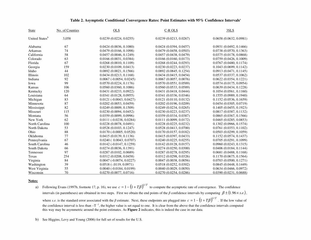
Table 2. Asymptotic Conditional Convergence Rates: Point Estimates with 95% Confidence Intervalsa

State No. of Counties OLS C-R OLS 3SLS

United Statesb 3,058 0.0239 (0.0224, 0.0255) 0.0239 (0.0213, 0.0267) 0.0658 (0.0632, 0.0981)

Alabama 67 0.0424 (0.0036, 0.1080) 0.0424 (0.0394, 0.0457) 0.0931 (0.0492, 0.1466)

Arkansas 74 0.0479 (0.0166, 0.1098) 0.0479 (0.0458, 0.0503) 0.0738 (0.0570, 0.1363)

California 58 0.0457 (0.0046, 0.1249) 0.0457 (0.0438, 0.0479) 0.0375 (0.0178, 0.0868)

Colorado 63 0.0166 (0.0031, 0.0384) 0.0166 (0.0160, 0.0173) 0.0759 (0.0426, 0.1009)

Florida 67 0.0268 (0.0010, 0.1109) 0.0268 (0.0244, 0.0293) 0.0767 (0.0480, 0.1174)

Georgia 159 0.0230 (0.0109, 0.0413) 0.0230 (0.0223, 0.0237) 0.1043 (0.0699, 0.1142)

Idaho 44 0.0892 (0.0021, 0.1566) 0.0892 (0.0845, 0.1254) 0.0913 (0.0471, 0.1145)

Illinois 102 0.0434 (0.0213, 0.1168) 0.0434 (0.0415, 0.0454) 0.0537 (0.0337, 0.1062)

Indiana 92 0.0067 (-0.0054, 0.0245) 0.0067 (0.0057, 0.0076) 0.0622 (0.0354, 0.1221)

Iowa 99 0.0570 (0.0224, 0.1176) 0.0570 (0.0551, 0.0589) 0.0574 (0.0175, 0.0954)

Kansas 106 0.0560 (0.0360, 0.1086) 0.0560 (0.0533, 0.0589) 0.0639 (0.0434, 0.1228)

Kentucky 120 0.0431 (0.0233, 0.0922) 0.0431 (0.0418, 0.0444) 0.1054 (0.0561, 0.1160)

Louisiana 64 0.0341 (0.0128, 0.0955) 0.0341 (0.0336, 0.0346) 0.1555 (0.0989, 0.1940)

Michigan 83 0.0121 (-0.0043, 0.0427) 0.0121 (0.0110, 0.0132) 0.1152 (0.0536, 0.1659)

Minnesota 87 0.0202 (0.0053, 0.0459) 0.0202 (0.0196, 0.0209) 0.0454 (0.0305, 0.0719)

Mississippi 82 0.0249 (0.0009, 0.1509) 0.0249 (0.0234, 0.0265) 0.1405 (0.0455, 0.1923)

Missouri 115 0.0230 (0.0094, 0.0452) 0.0230 (0.0223, 0.0237) 0.0817 (0.0387, 0.1132)

Montana 56 0.0359 (0.0099, 0.0996) 0.0359 (0.0334, 0.0387) 0.0865 (0.0367, 0.1566)

New York 62 0.0111 (-0.0238, 0.0284) 0.0111 (0.0099, 0.0172) 0.0465 (0.0285, 0.0853)

North Carolina 100 0.0228 (0.0078, 0.0491) 0.0228 (0.0225, 0.0232) 0.1302 (0.0966, 0.1574)

North Dakota 53 0.0528 (0.0103, 0.1247) 0.0528 (0.0413, 0.0700) 0.0761 (0.0353, 0.1102)

Ohio 88 0.0170 (-0.0005, 0.0520) 0.0170 (0.0157, 0.0182) 0.0503 (0.0299, 0.1059)

Oklahoma 77 0.0415 (0.0139, 0.1136) 0.0415 (0.0397, 0.0433) 0.1152 (0.0574, 0.1437)

Pennsylvania 67 0.0240 ( 0.0043, 0.0707) 0.0240 (0.0225, 0.0255) 0.0705 (0.0291, 0.1099)

South Carolina 46 0.0142 (-0.0147, 0.1259) 0.0142 (0.0128, 0.0157) 0.0960 (0.0243, 0.1315)

South Dakota 66 0.0274 (0.0036, 0.1391) 0.0274 (0.0250, 0.0300) 0.0406 (0.0184, 0.1144)

Tennessee 97 0.0287 (0.0102, 0.0689) 0.0287 (0.0278, 0.0295) 0.0681 (0.0488, 0.1168)

Texas 254 0.0312 (0.0208, 0.0458) 0.0312 (0.0298, 0.0326) 0.1170 (0.0675, 0.1564)

Virginia 84 0.0047 (-0.0074, 0.0227) 0.0047 (0.0038, 0.0056) 0.0703 (0.0500, 0.1271)

Washington 39 0.0518 (-.0119, 0.0971) 0.0518 (0.0252, 0.0302) 0.0845 (0.0448, 0.1449)

West Virginia 55 0.0040 (-0.0184, 0.0199) 0.0040 (0.0029, 0.0050) 0.0634 (0.0466, 0.0972)

Wisconsin 70 0.0270 (0.0077, 0.0716) 0.0270 (0.0254, 0.0286) 0.0390 (0.0231, 0.0688)

Notes:

a) Following Evans (1997b, footnote 17, p. 16), we use ( ) TTc

/111 β+−= to compute the asymptotic rate of convergence. The confidence

intervals (in parentheses) are obtained in two steps. First we obtain the end points of the β confidence intervals by computing ( ).e.s. ×± 961β ,

where s.e. is the standard error associated with the β estimate. Next, these endpoints are plugged into ( ) TTc

/111 β+−= . If the low value of

the confidence interval is less than –T -1, the higher value is set equal to one. It is clear from the above that the confidence intervals computed

this way may be asymmetric around the point estimates. As Figure 2 indicates, this is indeed the case in our data.

b) See Higgins, Levy and Young (2006) for full set of results for the U.S.

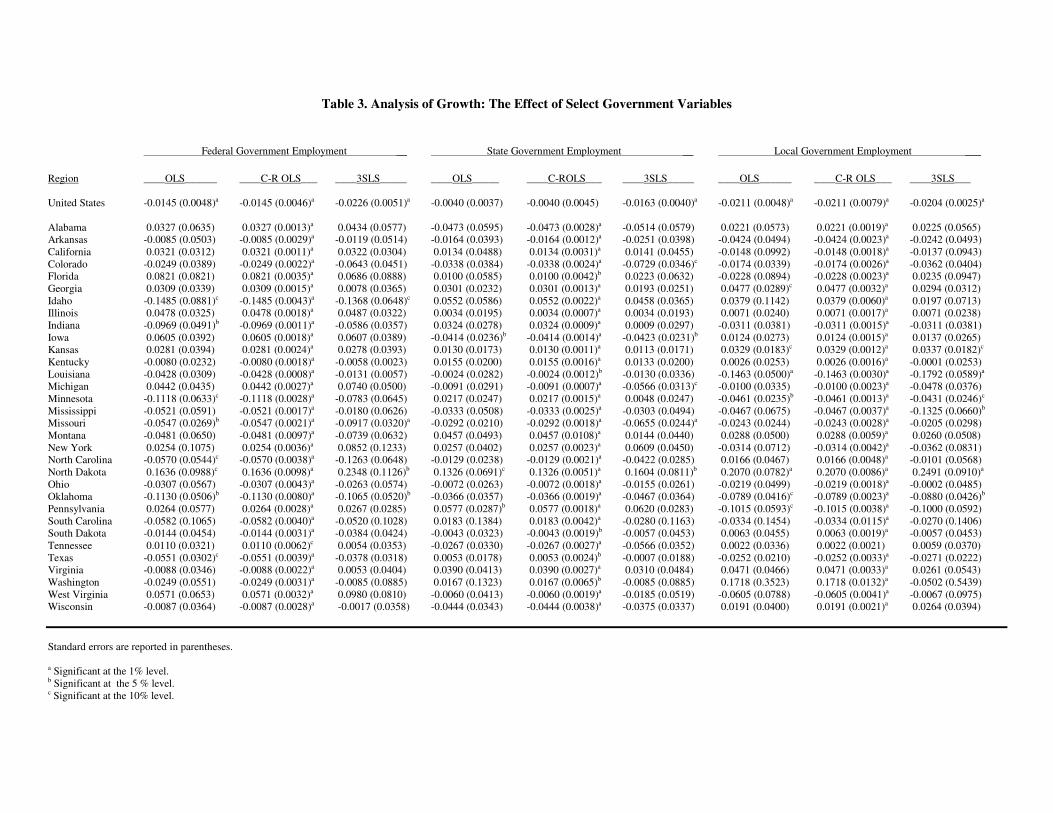
Table 3. Analysis of Growth: The Effect of Select Government Variables

Federal Government Employment __ State Government Employment __ Local Government Employment ___

Region ____OLS______ ____C-R OLS___ ____3SLS_____ ____OLS_____ ____C-ROLS___ ____3SLS_____ ____OLS______ ____C-R OLS___ ____3SLS___

United States -0.0145 (0.0048)a -0.0145 (0.0046)a -0.0226 (0.0051)a -0.0040 (0.0037) -0.0040 (0.0045) -0.0163 (0.0040)a -0.0211 (0.0048)a -0.0211 (0.0079)a -0.0204 (0.0025)a

Alabama 0.0327 (0.0635) 0.0327 (0.0013)a 0.0434 (0.0577) -0.0473 (0.0595) -0.0473 (0.0028)a -0.0514 (0.0579) 0.0221 (0.0573) 0.0221 (0.0019)a 0.0225 (0.0565)

Arkansas -0.0085 (0.0503) -0.0085 (0.0029)a -0.0119 (0.0514) -0.0164 (0.0393) -0.0164 (0.0012)a -0.0251 (0.0398) -0.0424 (0.0494) -0.0424 (0.0023)a -0.0242 (0.0493)

California 0.0321 (0.0312) 0.0321 (0.0011)a 0.0322 (0.0304) 0.0134 (0.0488) 0.0134 (0.0031)a 0.0141 (0.0455) -0.0148 (0.0992) -0.0148 (0.0018)a -0.0137 (0.0943)

Colorado -0.0249 (0.0389) -0.0249 (0.0022)a -0.0643 (0.0451) -0.0338 (0.0384) -0.0338 (0.0024)a -0.0729 (0.0346)c -0.0174 (0.0339) -0.0174 (0.0026)a -0.0362 (0.0404)

Florida 0.0821 (0.0821) 0.0821 (0.0035)a 0.0686 (0.0888) 0.0100 (0.0585) 0.0100 (0.0042)b 0.0223 (0.0632) -0.0228 (0.0894) -0.0228 (0.0023)a 0.0235 (0.0947)

Georgia 0.0309 (0.0339) 0.0309 (0.0015)a 0.0078 (0.0365) 0.0301 (0.0232) 0.0301 (0.0013)a 0.0193 (0.0251) 0.0477 (0.0289)c 0.0477 (0.0032)a 0.0294 (0.0312)

Idaho -0.1485 (0.0881)c -0.1485 (0.0043)a -0.1368 (0.0648)c 0.0552 (0.0586) 0.0552 (0.0022)a 0.0458 (0.0365) 0.0379 (0.1142) 0.0379 (0.0060)a 0.0197 (0.0713)

Illinois 0.0478 (0.0325) 0.0478 (0.0018)a 0.0487 (0.0322) 0.0034 (0.0195) 0.0034 (0.0007)a 0.0034 (0.0193) 0.0071 (0.0240) 0.0071 (0.0017)a 0.0071 (0.0238)

Indiana -0.0969 (0.0491)b -0.0969 (0.0011)a -0.0586 (0.0357) 0.0324 (0.0278) 0.0324 (0.0009)a 0.0009 (0.0297) -0.0311 (0.0381) -0.0311 (0.0015)a -0.0311 (0.0381)

Iowa 0.0605 (0.0392) 0.0605 (0.0018)a 0.0607 (0.0389) -0.0414 (0.0236)b -0.0414 (0.0014)a -0.0423 (0.0231)b 0.0124 (0.0273) 0.0124 (0.0015)a 0.0137 (0.0265)

Kansas 0.0281 (0.0394) 0.0281 (0.0024)a 0.0278 (0.0393) 0.0130 (0.0173) 0.0130 (0.0011)a 0.0113 (0.0171) 0.0329 (0.0183)c 0.0329 (0.0012)a 0.0337 (0.0182)c

Kentucky -0.0080 (0.0232) -0.0080 (0.0018)a -0.0058 (0.0023) 0.0155 (0.0200) 0.0155 (0.0016)a 0.0133 (0.0200) 0.0026 (0.0253) 0.0026 (0.0016)a -0.0001 (0.0253)

Louisiana -0.0428 (0.0309) -0.0428 (0.0008)a -0.0131 (0.0057) -0.0024 (0.0282) -0.0024 (0.0012)b -0.0130 (0.0336) -0.1463 (0.0500)a -0.1463 (0.0030)a -0.1792 (0.0589)a

Michigan 0.0442 (0.0435) 0.0442 (0.0027)a 0.0740 (0.0500) -0.0091 (0.0291) -0.0091 (0.0007)a -0.0566 (0.0313)c -0.0100 (0.0335) -0.0100 (0.0023)a -0.0478 (0.0376)

Minnesota -0.1118 (0.0633)c -0.1118 (0.0028)a -0.0783 (0.0645) 0.0217 (0.0247) 0.0217 (0.0015)a 0.0048 (0.0247) -0.0461 (0.0235)b -0.0461 (0.0013)a -0.0431 (0.0246)c

Mississippi -0.0521 (0.0591) -0.0521 (0.0017)a -0.0180 (0.0626) -0.0333 (0.0508) -0.0333 (0.0025)a -0.0303 (0.0494) -0.0467 (0.0675) -0.0467 (0.0037)a -0.1325 (0.0660)b

Missouri -0.0547 (0.0269)b -0.0547 (0.0021)a -0.0917 (0.0320)a -0.0292 (0.0210) -0.0292 (0.0018)a -0.0655 (0.0244)a -0.0243 (0.0244) -0.0243 (0.0028)a -0.0205 (0.0298)

Montana -0.0481 (0.0650) -0.0481 (0.0097)a -0.0739 (0.0632) 0.0457 (0.0493) 0.0457 (0.0108)a 0.0144 (0.0440) 0.0288 (0.0500) 0.0288 (0.0059)a 0.0260 (0.0508)

New York 0.0254 (0.1075) 0.0254 (0.0036)a 0.0852 (0.1233) 0.0257 (0.0402) 0.0257 (0.0023)a 0.0609 (0.0450) -0.0314 (0.0712) -0.0314 (0.0042)a -0.0362 (0.0831)

North Carolina -0.0570 (0.0544)c -0.0570 (0.0038)a -0.1263 (0.0648) -0.0129 (0.0238) -0.0129 (0.0021)a -0.0422 (0.0285) 0.0166 (0.0467) 0.0166 (0.0048)a -0.0101 (0.0568)

North Dakota 0.1636 (0.0988)c 0.1636 (0.0098)a 0.2348 (0.1126)b 0.1326 (0.0691)c 0.1326 (0.0051)a 0.1604 (0.0811)b 0.2070 (0.0782)a 0.2070 (0.0086)a 0.2491 (0.0910)a

Ohio -0.0307 (0.0567) -0.0307 (0.0043)a -0.0263 (0.0574) -0.0072 (0.0263) -0.0072 (0.0018)a -0.0155 (0.0261) -0.0219 (0.0499) -0.0219 (0.0018)a -0.0002 (0.0485)

Oklahoma -0.1130 (0.0506)b -0.1130 (0.0080)a -0.1065 (0.0520)b -0.0366 (0.0357) -0.0366 (0.0019)a -0.0467 (0.0364) -0.0789 (0.0416)c -0.0789 (0.0023)a -0.0880 (0.0426)b

Pennsylvania 0.0264 (0.0577) 0.0264 (0.0028)a 0.0267 (0.0285) 0.0577 (0.0287)b 0.0577 (0.0018)a 0.0620 (0.0283) -0.1015 (0.0593)c -0.1015 (0.0038)a -0.1000 (0.0592)

South Carolina -0.0582 (0.1065) -0.0582 (0.0040)a -0.0520 (0.1028) 0.0183 (0.1384) 0.0183 (0.0042)a -0.0280 (0.1163) -0.0334 (0.1454) -0.0334 (0.0115)a -0.0270 (0.1406)

South Dakota -0.0144 (0.0454) -0.0144 (0.0031)a -0.0384 (0.0424) -0.0043 (0.0323) -0.0043 (0.0019)b -0.0057 (0.0453) 0.0063 (0.0455) 0.0063 (0.0019)a -0.0057 (0.0453)

Tennessee 0.0110 (0.0321) 0.0110 (0.0062)c 0.0054 (0.0353) -0.0267 (0.0330) -0.0267 (0.0027)a -0.0566 (0.0352) 0.0022 (0.0336) 0.0022 (0.0021) 0.0059 (0.0370)

Texas -0.0551 (0.0302)c -0.0551 (0.0039)a -0.0378 (0.0318) 0.0053 (0.0178) 0.0053 (0.0024)b -0.0007 (0.0188) -0.0252 (0.0210) -0.0252 (0.0033)a -0.0271 (0.0222)

Virginia -0.0088 (0.0346) -0.0088 (0.0022)a 0.0053 (0.0404) 0.0390 (0.0413) 0.0390 (0.0027)a 0.0310 (0.0484) 0.0471 (0.0466) 0.0471 (0.0033)a 0.0261 (0.0543)

Washington -0.0249 (0.0551) -0.0249 (0.0031)a -0.0085 (0.0885) 0.0167 (0.1323) 0.0167 (0.0065)b -0.0085 (0.0885) 0.1718 (0.3523) 0.1718 (0.0132)a -0.0502 (0.5439)

West Virginia 0.0571 (0.0653) 0.0571 (0.0032)a 0.0980 (0.0810) -0.0060 (0.0413) -0.0060 (0.0019)a -0.0185 (0.0519) -0.0605 (0.0788) -0.0605 (0.0041)a -0.0067 (0.0975)

Wisconsin -0.0087 (0.0364) -0.0087 (0.0028)a -0.0017 (0.0358) -0.0444 (0.0343) -0.0444 (0.0038)a -0.0375 (0.0337) 0.0191 (0.0400) 0.0191 (0.0021)a 0.0264 (0.0394)

Standard errors are reported in parentheses.

a Significant at the 1% level. b Significant at the 5 % level. c Significant at the 10% level.

Table 4A. Analysis of Growth: The Effect of Select Education Variables

____ 9-11 Years and No More_ _____ _ High School Diploma_ _

Region _ _OLS __ __ C-R OLS __ ____ 3SLS_ _ _ _ _OLS __ _ C-R OLS __ ____ 3SLS_ __

United States -0.0209 (0.0033)a -0.0209 (0.0089)b -0.0204 (0.0035)a 0.0007 (0.0027) 0.0007 (0.0052) 0.0091 (0.0029)a

Alabama 0.0864 (0.0424)a 0.0864 (0.0029)a 0.0876 (0.0417)b 0.0147 (0.0484) 0.0147 (0.0036)a 0.0122 (0.0474)

Arkansas -0.0196 (0.0318) -0.0196 (0.0024)a -0.0181 (0.0325) 0.0096 (0.0325) 0.0096 (0.0023)a 0.0199 (0.0327)

California -0.0662 (0.0744) -0.0662 (0.0105)a -0.0659 (0.0724) -0.0395 (0.0042) -0.0395 (0.0026)a -0.0395 (0.0412)

Colorado 0.1174 (0.0424)a 0.1174 (0.0046)a 0.1323 (0.0510)a 0.0181 (0.0282) 0.0181 (0.0015)a 0.0621 (0.0307)b

Florida -0.1329 (0.0901) -0.1329 (0.0069)a -0.0219 (0.0846) 0.0351 (0.0697) 0.0351 (0.0096)a 0.0622 (0.0846)

Georgia -0.0097 (0.0142) -0.0097 (0.0022)a 0.0077 (0.0150) 0.0028 (0.0161) 0.0028 (0.0031) 0.0114 (0.0150)

Idaho 0.0530 (0.0807) 0.0530 (0.0037)a 0.0507 (0.0751) 0.1074 (0.0465)b 0.1074 (0.0021)a 0.1085 (0.0433)b

Illinois -0.0585 (0.0189)a -0.0585 (0.0019)a -0.0586 (0.0187)a -0.0102 (0.0112) -0.0102 (0.0014)a -0.0103 (0.0106)

Indiana -0.0454 (0.0238)c -0.0454 (0.0018)a -0.0327 (0.0263) -0.0440 (0.0158)a -0.0440 (0.0012)a -0.0220 (0.0165)

Iowa -0.0242 (0.0248) -0.0242 (0.0022)a -0.0235 (0.0244) 0.0085 (0.0129) 0.0085 (0.0010)a 0.0084 (0.0128)

Kansas -0.0166 (0.0218) -0.0166 (0.0018)a -0.0151 (0.0216) 0.0518 (0.0125)a 0.0518 (0.0016)a 0.0526 (0.0124)a

Kentucky 0.0051 (0.0266) 0.0051 (0.0032) 0.0039 (0.0267) 0.0443 (0.0181)b 0.0443 (0.0018)a 0.0474 (0.0179)a

Louisiana -0.0012 (0.0236) -0.0012 (0.0022) 0.0100 (0.0280) -0.0253 (0.0175) -0.0253 (0.0024)a -0.0239 (0.0209)

Michigan -0.0312 (0.0279) -0.0312 (0.0028)a -0.0347 (0.0326) -0.0111 (0.0222) -0.0111 (0.0016)a -0.0040 (0.0258)

Minnesota -0.0076 (0.0319) -0.0076 (0.0030)b -0.0167 (0.0331) 0.0157 (0.0319) 0.0157 (0.0018)a 0.0160 (0.0185)

Mississippi -0.0055 (0.0311) -0.0055 (0.0027)b 0.0070 (0.0334) -0.0705 (0.0419)c -0.0705 (0.0026)a -0.0900 (0.0448)b

Missouri -0.0158 (0.0232) -0.0158 (0.0016)a -0.0256 (0.0283) -0.0151 (0.0152) -0.0151 (0.0020)a 0.0172 (0.0174)

Montana -0.1558 (0.0800)c -0.1558 (0.0043)a -0.1496 (0.0813)c -0.0280 (0.0432) -0.0280 (0.0038)a -0.0138 (0.0426)

New York 0.0238 (0.0393) 0.0238 (0.0066)a 0.0352 (0.0456) -0.0392 (0.0428) -0.0392 (0.0029)a -0.0703 (0.0486)

North Carolina 0.0178 (0.0186) 0.0178 (0.0025)a 0.0317 (0.0225) 0.0074 (0.0178) 0.0074 (0.0024)a 0.0223 (0.0215)

North Dakota -0.0341 (0.0479) -0.0341 (0.0025)a -0.0270 (0.0566) -0.0506 (0.0390) -0.0506 (0.0037)a -0.0304 (0.0454)

Ohio 0.0279 (0.0286) 0.0279 (0.0032)a 0.0221 (0.0287) -0.0311 (0.0177)c -0.0311 (0.0013)a -0.0284 (0.0178)

Oklahoma -0.0064 (0.0367) -0.0064 (0.0026)b -0.0036 (0.0378) 0.0453 (0.0241)c 0.0453 (0.0017)a 0.0608 (0.0234)a

Pennsylvania 0.0063 (0.0276) 0.0063 (0.0022)a 0.0058 (0.0276) -0.0188 (0.0197) -0.0188 (0.0020)a -0.0224 (0.0193)

South Carolina -0.0298 (0.0514) -0.0298 (0.0026)a -0.0225 (0.0487) -0.0103 (0.0898) -0.0103 (0.0033)a -0.0169 (0.0865)

South Dakota -0.0764 (0.0340)b -0.0764 (0.0027)a -0.0675 (0.0339)b 0.0093 (0.0209) 0.0093 (0.0016)a 0.0166 (0.0205)

Tennessee -0.0146 (0.0277) -0.0146 (0.0035)a 0.0044 (0.0299) 0.0149 (0.0277) 0.0149 (0.0027)a 0.0151 (0.0305)

Texas -0.0467 (0.0116)c -0.0467 (0.0014)a -0.0544 (0.0122)a 0.0109 (0.0126) 0.0109 (0.0037)a 0.0072 (0.0134)

Virginia 0.0145 (0.0228) 0.0145 (0.0016)a 0.0180 (0.0267) 0.0181 (0.0276) 0.0181 (0.0017)a 0.0445 (0.0315)

Washington -0.1776 (0.2789) -0.1776 (0.0082)a -0.0318 (0.4374) -0.3253 (0.2056) -0.3253 (0.0057)a 0.0061 (0.2082)

West Virginia 0.0073 (0.0493) 0.0073 (0.0017)a 0.0421 (0.0609) -0.0708 (0.0406)c -0.0708 (0.0018)a -0.0225 (0.0482)

Wisconsin -0.0325 (0.0313) -0.0325 (0.0026)a -0.0248 (0.0304) -0.0288 (0.0172)c -0.0288 (0.0015)a -0.0268 (0.0164)


a Significant at 1% level. b Significant at 5% level. c Significant at 10% level.

Table 4B. Analysis of Growth: The Effect of Select Education Variables

Some College Education Bachelor Degree or Higher _

Region _ _OLS __ __ C-R OLS __ ____ 3SLS_ _ _ _ _OLS __ _ C-R OLS __ ____ 3SLS_ __

United States -0.0106 (0.0056)c -0.0106 (0.0089) -0.0014 (0.0061) 0.0424 (0.0058)a 0.0424 (0.0108)a 0.0701 (0.0061)a

Alabama 0.1202 (0.0993) 0.1202 (0.0107)a 0.1359 (0.0911) 0.0354 (0.0661) 0.0354 (0.0042)a 0.0350 (0.0653)

Arkansas 0.0249 (0.0684) 0.0249 (0.0040)a 0.0279 (0.0700) 0.1137 (0.0833) 0.1137 (0.0099)a 0.1475 (0.0826)c

California 0.0808 (0.0781) 0.0808 (0.0066)a 0.0808 (0.0749) 0.0901 (0.0592) 0.0901 (0.0037)a 0.0918 (0.0469)c

Colorado 0.1150 (0.0584)b 0.1150 (0.0081)a 0.0674 (0.0687) 0.0725 (0.0374)b 0.0725 (0.0036)a 0.1298 (0.0409)a

Florida 0.0622 (0.1298) 0.0625 (0.0089)a 0.1802 (0.1308) -0.0541 (0.1026) -0.0541 (0.0091)a 0.0971 (0.0893)

Georgia 0.0776 (0.0413)c 0.0776 (0.0037)a 0.0634 (0.0449) 0.0260 (0.0316) 0.0260 (0.0028)a 0.0279 (0.0339)

Idaho -0.0041 (0.0637) -0.0041 (0.0057) -0.0093 (0.0552) 0.0529 (0.1543) 0.0529 (0.0168)a 0.0372 (0.1274)

Illinois 0.0155 (0.0315) 0.0155 (0.0038)a 0.0154 (0.0311) 0.0401 (0.0322) 0.0401 (0.0027)a 0.0398 (0.0308)

Indiana 0.1215 (0.0529)b 0.1215 (0.0034)a 0.1230 (0.0591)b -0.0434 (0.0508) -0.0434 (0.0032)a 0.0373 (0.0516)

Iowa 0.0098 (0.0280) 0.0098 (0.0028)a 0.0111 (0.0271) -0.0187 (0.0319) 0.0351 (0.0032)a -0.0193 (0.0316)

Kansas 0.0009 (0.0207) 0.0009 (0.0015) 0.0051 (0.0198) 0.0351 (0.0266) 0.0351 (0.0016)a 0.0382 (0.0262)

Kentucky 0.0595 (0.0423) 0.0595 (0.0038)a 0.0630 (0.0423) 0.0492 (0.0457) 0.0492 (0.0040)a 0.0578 (0.0452)

Louisiana 0.0497 (0.0544) 0.0497 (0.0048)a 0.1022 (0.0627) 0.0306 (0.0517) 0.0306 (0.0032)a 0.0459 (0.0616)

Michigan -0.0189 (0.0480) -0.0189 (0.0039)a 0.0173 (0.0551) 0.0316 (0.0343) 0.0316 (0.0033)a 0.0926 (0.0362)b

Minnesota 0.0289 (0.0358) 0.0289 (0.0031)a 0.0472 (0.0365) 0.0399 (0.0408) 0.0399 (0.0031)a 0.0414 (0.0426)

Mississippi 0.0313 (0.0629) 0.0313 (0.0048)a -0.0249 (0.0649) -0.0905 (0.0789) -0.0905 (0.0061)a -0.0002 (0.0788)

Missouri -0.0103 (0.0321) -0.0103 (0.0046)a -0.0288 (0.0391) 0.0653 (0.0333)b 0.0653 (0.0042)a 0.1259 (0.0388)a

Montana -0.0002 (0.0420) -0.0002 (0.0035) 0.0131 (0.0415) 0.0106 (0.0534) 0.0106 (0.0022)a 0.0265 (0.0529)

New York 0.0171 (0.0757) 0.0171 (0.0034)a 0.0453 (0.0877) 0.0627 (0.0624) 0.0627 (0.0026)a 0.1673 (0.0616)a

North Carolina 0.0091 (0.0410) 0.0091 (0.0036)b -0.0282 (0.0495) 0.0446 (0.0344) 0.0446 (0.0030)a 0.1161 (0.0391)a

North Dakota 0.1271 (0.1270)b 0.1271 (0.0053)a 0.1493 (0.0666)b -0.0158 (0.0981) -0.0158 (0.0142) -0.0148 (0.1162)

Ohio 0.1224 (0.0530)b 0.1224 (0.0042)a 0.1453 (0.0516)a 0.0664 (0.0439) 0.0664 (0.0044)a 0.0743 (0.0442)c

Oklahoma 0.0230 (0.0498) 0.0230 (0.0054)a 0.0538 (0.0484) 0.0289 (0.0389) 0.0289 (0.0053)a 0.0332 (0.0400)

Pennsylvania 0.0108 (0.0560) 0.0108 (0.0060)c 0.0148 (0.0558) 0.1756 (0.0497)a 0.1756 (0.0042)a 0.1972 (0.0443)

South Carolina 0.1544 (0.2155) 0.1544 (0.0105)a 0.1995 (0.1984) -0.0270 (0.2123) -0.0270 (0.0086)a 0.0369 (0.1838)

South Dakota 0.0405 (0.0449) 0.0405 (0.0030)a 0.0493 (0.0451) -0.0389 (0.0569) -0.0389 (0.0037)a -0.0245 (0.0567)

Tennessee -0.0672 (0.0585) -0.0672 (0.0060)a -0.0728 (0.0644) 0.1118 (0.0551)b 0.1118 (0.0091)a 0.1764 (0.0586)a

Texas 0.0372 (0.0208) 0.0372 (0.0052)a 0.0390 (0.0220)b 0.0211 (0.0243) 0.0211 (0.0028)a 0.0032 (0.0252)

Virginia -0.0588 (0.0709) -0.0588 (0.0070)a -0.0764 (0.0830) 0.0611 (0.0528) 0.0611 (0.0052)a 0.1354 (0.0583)b

Washington -0.1544 (0.1287) -0.1544 (0.0024)a 0.0499 (0.1331) 0.0631 (0.3615) 0.0631 (0.0078)a -0.0076 (0.5835)

West Virginia 0.0119 (0.0816) 0.0119 (0.0032)a -0.0145 (0.1025) 0.0127 (0.1123) 0.0127 (0.0078) 0.1077 (0.1374)

Wisconsin 0.0116 (0.0348) 0.0116 (0.0016)a 0.0227 (0.0331) 0.0703 (0.0424) 0.0703 (0.0029)a 0.0921 (0.0368)b



Table 5. Analysis of Growth: The Effect of Select Industry Composition Variables

Finance, Insurance, and Real Estate _ Educational Services _ Entertainment and Recreational Services

Region ____OLS___ ____C-R OLS___ ____3SLS___ ____OLS___ ____C-R OLS___ ____3SLS___ ____OLS___ ____C-R OLS___ ____3SLS___

United States 0.0632 (0.0117)a 0.0632 (0.0233)a 0.0731 (0.0125)a -0.0257 (0.0082)a -0.0257 (0.0060)a -0.0445 (0.0087) 0.0272 (0.0154)c 0.0272 (0.0230) 0.0335 (0.0166)b

Alabama 0.2482 (0.1525)c 0.2482 (0.0057)a 0.2642 (0.1458)c -0.1586 (0.1912) -0.1586 (0.0103)a -0.1835 (0.1798) 0.0127 (0.3372) 0.0127 (0.0212) 0.0165 (0.3325)

Arkansas 0.0146 (0.1124) 0.0146 (0.0064)b 0.0155 (0.1151) 0.0972 (0.0780) 0.0972 (0.0037)a 0.1070 (0.0796) -0.1725 (0.1915) -0.1725 (0.0196)a -0.1336 (0.1945)

California 0.0625 (0.0956) 0.0625 (0.0075)a 0.0639 (0.0892) 0.0238 (0.1275) 0.0238 (0.0195) 0.0254 (0.1206) 0.1749 (0.0744)b 0.1749 (0.0040)a 0.1751 (0.0724)b

Colorado 0.1602 (0.0885)c 0.1602 (0.0077)a 0.0962 (0.1047) 0.1536 (0.0843)c 0.1536 (0.0061)a 0.1387 (0.1018) 0.0655 (0.1162) 0.0655 (0.0080)a 0.1410 (0.1162)

Florida 0.1226 (0.1210) 0.1226 (0.0094)a 0.1121 (0.1312) -0.2992 (0.2080) -0.2992 (0.0235)a -0.4666 (0.2131)b 0.2011 (0.2475) 0.2011 (0.0183)a 0.1682 (0.2680)

Georgia -0.0375 (0.0714) -0.0375 (0.0055)a -0.0513 (0.0776) 0.0540 (0.0665) 0.0540 (0.0039)a 0.0409 (0.0723) 0.2172 (0.1262)c 0.2172 (0.0088)a 0.2617 (0.1369)b

Idaho -0.2663 (0.2141) -0.2663 (0.0133)a -0.2609 (0.1993) -0.3225 (0.2219) -0.3225 (0.0192)a -0.2925 (0.1613)c -0.1767 (0.3483) -0.1767 (0.0415)a -0.1881 (0.3230)

Illinois 0.1293 (0.0487)a 0.1293 (0.0076)a 0.1292 (0.0482)a -0.1407 (0.0684)a -0.1407 (0.0024)a -0.1407 (0.0678)b 0.4266 (0.1635)a 0.4266 (0.0168)a 0.4265 (0.1622)a

Indiana -0.0809 (0.0849) -0.0809 (0.0049)a -0.0055 (0.0923) -0.2438 (0.1008)b -0.2438 (0.0065)a -0.3410 (0.1090)a 0.0554 (0.2051) 0.0554 (0.0270)b 0.1228 (0.2283)

Iowa 0.1280 (0.0920) 0.1280 (0.0082)a 0.1312 (0.0902) -0.0334 (0.0484) -0.0334 (0.0049)a -0.0340 (0.0479) 0.1931 (0.1870) 0.1931 (0.0154)a 0.1975 (0.1845)

Kansas 0.0819 (0.0611) 0.0819 (0.0051)a 0.0827 (0.0608) -0.0184 (0.0387) -0.0184 (0.0042)a -0.0191 (0.0386) 0.0667 (0.1089) 0.0667 (0.0079)a 0.0587 (0.1080)

Kentucky -0.0590 (0.0636) -0.0590 (0.0042)a -0.0616 (0.0638) 0.0568 (0.0635) 0.0568 (0.0040)a 0.0445 (0.0628) 0.0868 (0.1512) 0.0868 (0.0111)a 0.0597 (0.1499)

Louisiana -0.3930 (0.1158)a -0.3930 (0.0086)a -0.4513 (0.1373)a 0.0923 (0.0795) 0.0923 (0.0055)a 0.0386 (0.0935) 0.1019 (0.2055) 0.1019 (0.0102)a 0.3692 (0.2291)

Michigan 0.1550 (0.0927)c 0.1550 (0.0104)a 0.1718 (0.1080) -0.0541 (0.0907) -0.0541 (0.0082)a -0.0447 (0.1057) -0.0656 (0.2009) -0.0656 (0.0311)b -0.1524 (0.2330)

Minnesota -0.0210 (0.0973) -0.0210 (0.0095)b 0.0711 (0.0932) -0.0089 (0.0653) -0.0089 (0.0084) -0.0684 (0.0630) -0.0834 (0.1741) -0.0834 (0.0177)a -0.0356 (0.1807)

Mississippi 0.1893 (0.1720) 0.1893 (0.0111)a 0.1215 (0.1846) -0.2570 (0.1238)b -0.2570 (0.0140)a -0.2330 (0.1338)c 0.9804 (0.3651)a 0.9804 (0.0347)a 0.9807 (0.3951)a

Missouri 0.0047 (0.0555) 0.0047 (0.0075) -0.0006 (0.0677) -0.0088 (0.0531) -0.0088 (0.0064) 0.0324 (0.0643) -0.0965 (0.1564) -0.0965 (0.0157)a -0.1621 (0.1905)

Montana 0.1329 (0.1171) 0.1329 (0.0133)a 0.1322 (0.1192) -0.0559 (0.0714) -0.0559 (0.0031)a -0.0418 (0.0718) 0.2509 (0.1795) 0.2509 (0.0203)a 0.2599 (0.1825)

New York 0.0388 (0.0906) 0.0388 (0.0081)a 0.1049 (0.1027) 0.0081 (0.1500) 0.0081 (0.0143) -0.0412 (0.1739) 0.4809 (0.3271) 0.4809 (0.0234)a 0.9166 (0.3458)a

North Carolina 0.0002 (0.0979) 0.0002 (0.0095) -0.0582 (0.1190) 0.1124 (0.0923) 0.1124 (0.0068)a 0.1193 (0.1128) 0.2905 (0.1658)c 0.2905 (0.0110)a 0.2682 (0.2026)

North Dakota 0.5098 (0.1772)a 0.5098 (0.0112)a 0.6835 (0.1973)a 0.0844 (0.1305) 0.0844 (0.0111)a 0.0069 (0.1513) 0.4364 (0.2406)c 0.4364 (0.0293)a 0.8632 (0.2241)a

Ohio -0.0762 (0.1047) -0.0762 (0.0111)a -0.0512 (0.1049) 0.0552 (0.1002) 0.0552 (0.0045)a 0.0621 (0.1015) 0.2190 (0.2161) 0.2190 (0.0102)a 0.2317 (0.2190)

Oklahoma -0.1433 (0.0858)c -0.1433 (0.0148)a -0.1056 (0.0859) 0.1124 (0.0802) 0.1124 (0.0097)a 0.1192 (0.0826) -0.2395 (0.2164) -0.2395 (0.0171)a -0.2504 (0.2230)

Pennsylvania -0.0722 (0.0926) -0.0722 (0.0046)a -0.0729 (0.0925) -0.2894 (0.1356)b -0.2894 (0.0105)a -0.2877 (0.1359) 0.1728 (0.3373) 0.1728 (0.0314)a 0.1829 (0.3367)

South Carolina -0.0651 (0.3950) -0.0651 (0.0100)a -0.1697 (0.3516) 0.1028 (0.4210) 0.1028 (0.0182)a 0.0355 (0.3962) -0.1874 (0.5102) -0.1874 (0.0196)a -0.2592 (0.4834)

South Dakota 0.0224 (0.0995) 0.0224 (0.0122)c 0.0191 (0.1009) 0.0217 (0.0705) 0.0217 (0.0060)a 0.0185 (0.0715) -0.1549 (0.1672) -0.1549 (0.0154)a -0.1697 (0.1693)

Tennessee 0.3037 (0.1073)a 0.3037 (0.0125)a 0.2818 (0.1180)b 0.1126 (0.0953) 0.1126 (0.0141)a 0.0832 (0.1046) -0.4127 (0.2956) -0.4127 (0.0194)a -0.3183 (0.3242)

Texas 0.0899 (0.0551) 0.0899 (0.0082)a 0.1402 (0.0575)b -0.0054 (0.0423) -0.0054 (0.0083) -0.0419 (0.0441) -0.0295 (0.1200) -0.0295 (0.0211) -0.0331 (0.1270)

Virginia 0.0397 (0.1063) 0.0397 (0.0711) 0.1585 (0.1202) -0.2021 (0.0923)b -0.2021 (0.0048)a -0.2007 (0.1082)b 0.0121 (0.2363) 0.0121 (0.0229) 0.0617 (0.2767)

Washington 0.2547 (0.3233) 0.2547 (0.0093)a -0.0507 (0.4659) 0.7953 (0.8042) 0.7953 (0.0086)a 0.3685 (0.9599) -0.6752 (0.6909) -0.6752 (0.0334)a 0.1019 (0.9390)

West Virginia 0.0747 (0.1321) 0.0747 (0.0076)a 0.1688 (0.1632) 0.0943 (0.1278) 0.0943 (0.0082)a -0.0228 (0.1556) 0.0980 (0.2026) 0.0980 (0.0073)a 0.3967 (0.2318)c

Wisconsin 0.0192 (0.0813) 0.0192 (0.0064)a 0.0213 (0.0813) -0.0094 (0.0992) -0.0094 (0.0058) -0.0209 (0.0986) -0.0401 (0.2274) -0.0401 (0.0318) -0.0177 (0.2266)



1

Referee’s Appendix

I. Inconsistency of OLS Estimates

The method of ordinary least squares (OLS) could be used to infer the values of β and γ

in equation (2.3). However, Evans (1997b) states that the OLS estimates obtained from (2.3) are

unlikely to be consistent.1 In order to demonstrate this inconsistency, Evans first specifies a

general autoregressive moving average (ARMA) data-generating process for nty :

(1A) ∑=

−−− +−+=−q

iitnnittnnntnt ayay

1,11, )( εθλδ

with

(2A) nnnn x ωξκδ +′+=

where ntε is a zero-mean, covariance stationary error process independently distributed over

time and across economies. The error term, ntε , is uncorrelated with nx , nλ is an autoregressive

parameter which lies on ]1,0( , and nqn θθ ...0 satisfy the restriction 10 =nθ . As such, tnt ay − will

also have an autoregressive representation and will be covariance stationary if nλ <1 or

difference stationary if 1=nλ . The common time-specific effect experienced by every economy

is represented by the term ta . Evans assumes that ta∆ is covariance stationary and independent

of ntε .

The common trend ta for all the y variables will be the sole catalyst of economic growth

in all economies if nλ <1. In this case, growth is exogenous and economies would follow a

balanced-growth path. If nλ =1, on the other hand, then economy n will grow endogenously

since nty diverges from ta and the y variables of all remaining economies. The parameter nδ

controls for the relative height of economy n ’s balanced growth path if all the λ s are less than

one. If 1=nλ , then nδ controls for economy n ’s relative growth rate. The error term nω

measures the portion of nδ that is not explained by nx . This error term is assumed to be

1 This appendix borrows heavily from Evans (1997b), which can be consulted for further details. Because Evans (1997b) is unpublished, this appendix is included here for the convenience of the reader but, it is not intended for publication.

2

uncorrelated with nx . The inequality nλ <1 will hold for an economy described by the

neoclassical growth model.

Solving equation (1A) backward from year T to year 0, substituting from equation (2A),

and rearranging produces

(3A)

[ ]

∑ ∑

∑ ∑−

=−

+=

−

−

=−

=

−

⎟⎟⎠

⎞⎜⎜⎝

⎛⎟⎟⎠

⎞⎜⎜⎝

⎛+

⎟⎟⎠

⎞⎜⎜⎝

⎛+

−−′++=

1

0,

1

1

0,

,min

00

11

q

iin

q

ijnj

jn

in

Tn

T

iiTn

qi

jnj

jn

in

n

nnnnnnnn

T

Txyg

εθλλλ

εθλλγωβ

γβα

where T

Tn

n1−

=λ

β , n

nnn λ

ξβγ

−−

=1

, and

⎟⎟⎠

⎞⎜⎜⎝

⎛−

+−

−=

nn

Tn a

T

aa

λκ

βα

10

0 . If 0<nβ , then economy n

grows exogenously ( )1<nλ . On the other hand, if 0=nβ , then economy n grows

endogenously ( )1=nλ .

Now consider a special case in which every intercept nδ is completely explained by the

county characteristics included in nx ωn = 0,∀n( ) and every series tnt ay − is a first-order auto-

regression ( )0=q . Under these restrictions equation (3A) reduces to:

(4A) ∑−

=−+′++=

1

0,0

1 T

iiTn

innnnnnn T

xyg ελγβα

The estimator for β can then be obtained in two steps. First, regress 0ny on an intercept and nx

to obtain the residual nr and then regress ng on nr . (This is simply the OLS estimator of β.)

Each term in ∑−

=−

1

0,

1 T

iiTn

inTελ is uncorrelated with the intercept, ny , nx and the residual nr . As a

result, one has

(5A) ∑

∑∑∑

=∞→

=∞→=∞→=∞→

∞→

′++= N

nn

N

N

nnnn

N

N

nnnn

N

N

nnn

N

N rN

p

xrN

pyrN

prN

pp

1

2

111

1lim

1lim1lim1limˆlim

γβαβ

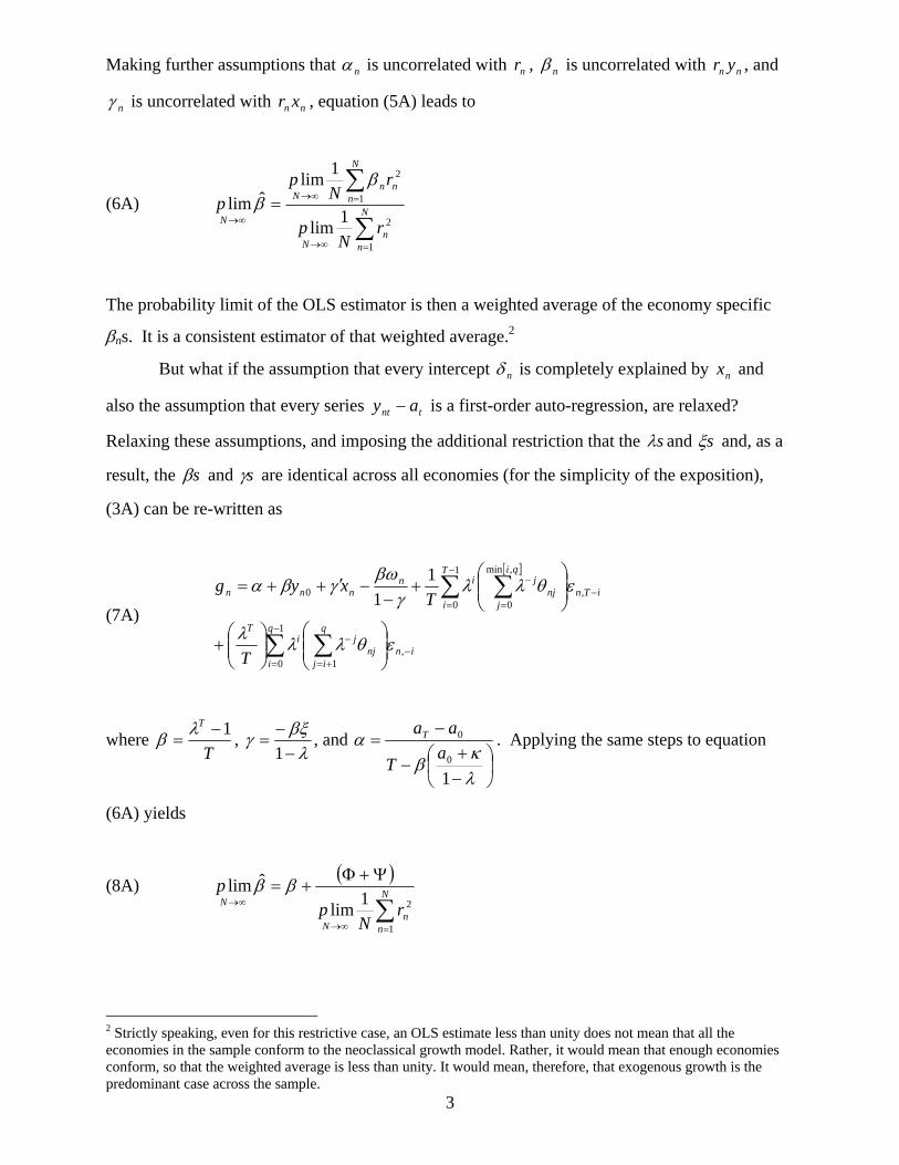
3

Making further assumptions that nα is uncorrelated with nr , nβ is uncorrelated with nn yr , and

nγ is uncorrelated with nn xr , equation (5A) leads to

(6A) ∑

∑

=∞→

=∞→

∞→= N

nn

N

N

nnn

N

N rN

p

rN

pp

1

2

1

2

1lim

1limˆlim

ββ

The probability limit of the OLS estimator is then a weighted average of the economy specific

βns. It is a consistent estimator of that weighted average.2

But what if the assumption that every intercept nδ is completely explained by nx and

also the assumption that every series tnt ay − is a first-order auto-regression, are relaxed?

Relaxing these assumptions, and imposing the additional restriction that the sλ and sξ and, as a

result, the sβ and sγ are identical across all economies (for the simplicity of the exposition),

(3A) can be re-written as

(7A)

[ ]

∑ ∑

∑ ∑−

=−

+=

−

−

=−

=

−

⎟⎟⎠

⎞⎜⎜⎝

⎛⎟⎟⎠

⎞⎜⎜⎝

⎛+

⎟⎟⎠

⎞⎜⎜⎝

⎛+

−−′++=

1

0,

1

1

0,

,min

00

11

q

iin

q

ijnj

jiT

T

iiTn

qi

jnj

jinnnn

T

Txyg

εθλλλ

εθλλγ

βωγβα

where T

T 1−=

λβ , λ

βξγ−

−=

1, and

⎟⎠⎞

⎜⎝⎛

−+

−

−=

λκ

βα

10

0

aT

aaT . Applying the same steps to equation

(6A) yields

(8A) ( )

∑=∞→

∞→

Ψ+Φ+= N

nn

N

N rN

pp

1

21lim

ˆlim ββ

2 Strictly speaking, even for this restrictive case, an OLS estimate less than unity does not mean that all the economies in the sample conform to the neoclassical growth model. Rather, it would mean that enough economies conform, so that the weighted average is less than unity. It would mean, therefore, that exogenous growth is the predominant case across the sample.

4

where ∑ ∑∑=

−++−

−

=∞→ ⎥⎥⎦

⎤

⎢⎢⎣

⎡⎟⎟⎠

⎞⎜⎜⎝

⎛=Φ

N

ninnijn

jq

i

i

N

T

rNIp

T 1,1,

1

0lim εθλλλ and ∑

∞→−−=Ψ nn

Nr

Np ω

λβ 1lim

1.

As a result, equation (8A) implies that βlim∞→N

p differs from β if either q > 0 (ynt – at is not a

first-order AR process) or the cross-sectional variance of nω is positive (not all cross-sectional

heterogeneity is accounted for). In other words, the OLS estimator is inconsistent unless (a) the

log of income per capita has an identical first-order AR representation across economies, and (b)

all cross-section heterogeneity is controlled for.

Evans shows that the resulting bias from q > 0 is likely to be negligible in practice but the

bias resulting from a positive cross-sectional variance for nω can be substantial. This is

essentially an omitted variable bias. Evans demonstrates that

(9A) p limN →∞

ˆ β =var y | x,ω( )var y | x( )

⎡

⎣ ⎢ ⎢

⎤

⎦ ⎥ ⎥ β

and

(10A) p limN →∞

ˆ γ =var y | x,ω( )var y | x( )

⎡

⎣ ⎢ ⎢

⎤

⎦ ⎥ ⎥ γ .

The bracketed portions in equations (9A) and (10A) are the ratio of the cross-sectional variance

of 0ny conditional on both nx and nω to the cross-sectional variance of 0ny on nx . As such, β

and γ will be biased towards zero unless the xs are able to control for a large portion of the

cross-economy variation in the ys .

The intuition here is that if a large portion of the growth of per capita income is explained

by variables left out of the OLS regression, then the estimate of the convergence effect will be

biased. In general, omitted variable bias can be either positive or negative. However, in this

case, theoretically, the bias is negative. Evans (1997b, Tables on p. 11 and p. 15) estimates β for

Mankiw, et al.’s (1992) international data using both the OLS, which yields inconsistent

estimates, and the 2SLS approach (as outlined in section 2), which yields consistent estimates of

both β and γ. He finds that the 2SLS estimate implies a conditional convergence rate between 4

to 5 times as large as the OLS estimate. The bias produced by the OLS in this case, therefore, is

substantial.

Heterogeneous Convergence - Emory University

Documents

Transcript of Heterogeneous Convergence - Emory University