Hessian measures of semi-convex functions andapplications to support measures of convex bodies∗

Andrea Colesanti and Daniel Hug

Abstract

This paper originates from the investigation of support measures of convex bodies(sets of positive reach), which form a central subject in convex geometry and alsorepresent an important tool in related fields. We show that these measures are abso-lutely continuous with respect to Hausdorff measures of appropriate dimensions, andwe determine the Radon-Nikodym derivatives explicitly on sets of σ-finite Hausdorffmeasure. The results which we obtain in the setting of the theory of convex bodies(sets of positive reach) are achieved as applications of various new results on Hessianmeasures of convex (semi-convex) functions. Among these are a Crofton formula,results on the absolute continuity of Hessian measures, and a duality theorem whichrelates the Hessian measures of a convex function to those of the conjugate function.In particular, it turns out that curvature and surface area measures of a convex bodyK are the Hessian measures of special functions, namely the distance function andthe support function of K.

0 Introduction

The theory of curvature and surface area measures plays a central role in the classical theoryof convex bodies. The importance of these measures is due to the fact that they relateclassical convexity to integral and stochastic geometry, for which they are indispensibletools. But they are also relevant for such diverse subjects as the theory of valuations onconvex bodies [38], [3], [4], research on zonoids, projection functions and functional analyticcharacterizations of classes of convex bodies [26], [27], geometric tomography [22], or thestudy of isotropic positions of convex bodies [23], [24], and thus the local theory of Banachspaces. Despite the fact that these measures have a long tradition in convexity, some of thebasic questions only have been addressed quite recently and others have not been solved sofar; this can be seen, for instance, from the survey papers [39], [37] and the lecture notes[40].

∗AMS 1991 subject classification. Primary 52A20, 26B25; Secondary 53C65, 28A78.Key words and phrases. Hessian measure, support measure, curvature and surface area measure, Croftonformula, absolute continuity, Radon-Nikodym derivative, semi-convex function, set of positive reach, Haus-dorff measure.

1

2

The curvature and surface area measures, and also their common generalization, thesupport measures, contain essential local as well as global information about the shapeof the set with which they are associated. The investigation of the connection betweenmeasure theoretic properties of these measures and geometric properties of the underlyingsets represents a major theme in this field; see [40] and the survey given in Section 1 of [29].Another main topic is the study of integral geometric formulae such as principal kinematicformulae or Crofton formulae and their applications to stochastic geometry. Of course,curvature and surface area measures also lead to interesting and challenging questionsfrom a mainly measure theoretic point of view; in particular, various relationships betweenthese measures and Hausdorff measures have been analyzed.

The present paper originates from the investigation of properties of curvature and sur-face area measures of convex bodies. The main purpose is to establish absolute continuityresults of such measures with respect to Hausdorff measures of suitable dimensions, and tofind explicit expressions for the corresponding densities. The results that we obtain in thesetting of the theory of convex bodies are achieved as applications of new and more generalresults, presented in the first part of the paper, regarding Hessian measures of semi-convexfunctions. Hessian measures have only emerged quite recently, and most likely they havethe potential for a similar development as the classical curvature and surface area mea-sures. It is a major aim of this investigation to improve our knowledge of these measures,which is particularly rewarding, since it also leads to new insights into the existing theoryof curvature and surface area measures.

If K ⊂ Rd is a convex body, i.e. a non-empty compact convex set, then its curvaturemeasures Cj(K, ·), j ∈ 0, 1, . . . , d− 1, are Borel measures on Rd which are concentratedon the boundary ∂K of K and which generalize the notion of surface integrals of theelementary symmetric functions of the principal curvatures of ∂K. An analogous notionis the one of a surface area measure of K, denoted by Sj(K, ·), where j ∈ 0, 1, . . . , d− 1;the surface area measures are defined on the Borel sets of the unit sphere Sd−1, and forconvex bodies with sufficiently smooth support functions they correspond to integrals of theelementary symmetric functions of the principal radii of curvature. The concept of supportmeasures, or generalized curvature measures, represents a unified approach to curvature andsurface area measures. We refer the reader to the book [36] for a detailed presentation ofthese measures (see Chapter 4), for further references to the extensive literature on thesubject, as well as for a description of all notions of convex geometry for which no explicitdefinition is given here.

For special classes of convex bodies, such as polytopes or sufficiently smooth convexbodies, the properties of curvature and surface area measures are clear from the explicitrepresentations of these measures, which can be obtained in these particular cases. How-ever, the situation changes drastically when we consider arbitrary convex bodies. One ofthe general measure theoretic results, due to R. Schneider (see Theorem 4.6.5 in [36]),states that the measure Cj(K, ·) is absolutely continuous with respect to the j-dimensionalHausdorff measure Hj for every j ∈ 0, 1, . . . , d − 1; analogously, Sj(K, ·) is absolutelycontinuous with respect to Hd−j−1, for every j ∈ 0, 1, . . . , d−1 (see the Notes for Section4.6 in [36]). As a consequence, Cj(K, ·) and Sj(K, ·) possess Radon-Nikodym derivatives

3

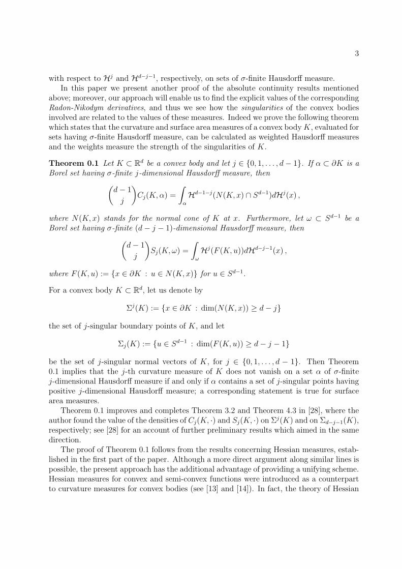
with respect to Hj and Hd−j−1, respectively, on sets of σ-finite Hausdorff measure.In this paper we present another proof of the absolute continuity results mentioned

above; moreover, our approach will enable us to find the explicit values of the correspondingRadon-Nikodym derivatives, and thus we see how the singularities of the convex bodiesinvolved are related to the values of these measures. Indeed we prove the following theoremwhich states that the curvature and surface area measures of a convex body K, evaluated forsets having σ-finite Hausdorff measure, can be calculated as weighted Hausdorff measuresand the weights measure the strength of the singularities of K.

Theorem 0.1 Let K ⊂ Rd be a convex body and let j ∈ 0, 1, . . . , d− 1. If α ⊂ ∂K is aBorel set having σ-finite j-dimensional Hausdorff measure, then(

d− 1

j

)Cj(K, α) =

∫α

Hd−1−j(N(K, x) ∩ Sd−1)dHj(x) ,

where N(K, x) stands for the normal cone of K at x. Furthermore, let ω ⊂ Sd−1 be aBorel set having σ-finite (d− j − 1)-dimensional Hausdorff measure, then(

d− 1

j

)Sj(K, ω) =

∫ω

Hj(F (K, u))dHd−j−1(x) ,

where F (K,u) := x ∈ ∂K : u ∈ N(K, x) for u ∈ Sd−1.

For a convex body K ⊂ Rd, let us denote by

Σj(K) := x ∈ ∂K : dim(N(K, x)) ≥ d− j

the set of j-singular boundary points of K, and let

Σj(K) := u ∈ Sd−1 : dim(F (K, u)) ≥ d− j − 1

be the set of j-singular normal vectors of K, for j ∈ 0, 1, . . . , d − 1. Then Theorem0.1 implies that the j-th curvature measure of K does not vanish on a set α of σ-finitej-dimensional Hausdorff measure if and only if α contains a set of j-singular points havingpositive j-dimensional Hausdorff measure; a corresponding statement is true for surfacearea measures.

Theorem 0.1 improves and completes Theorem 3.2 and Theorem 4.3 in [28], where theauthor found the value of the densities of Cj(K, ·) and Sj(K, ·) on Σj(K) and on Σd−j−1(K),respectively; see [28] for an account of further preliminary results which aimed in the samedirection.

The proof of Theorem 0.1 follows from the results concerning Hessian measures, estab-lished in the first part of the paper. Although a more direct argument along similar lines ispossible, the present approach has the additional advantage of providing a unifying scheme.Hessian measures for convex and semi-convex functions were introduced as a counterpartto curvature measures for convex bodies (see [13] and [14]). In fact, the theory of Hessian

4

measures now appears to be more general and flexible, since it yields the correspondingresults for curvature and surface area measures by applying results for Hessian measures tospecial functions related to a convex body, like the distance function, the support functionand the convex characteristic function. Moreover, an additional interesting and unexpectedfeature in the theory of Hessian measures, as presented here, is a notion of duality relatedto the conjugation of convex functions, for which no correspondence exists in the theoryof support measures of convex bodies.

For a semi-convex function u defined in an open convex subset Ω of Rd, the Hessianmeasures Fj(u, ·), j ∈ 0, 1, . . . , d, of u can be obtained as coefficients of a local Steinertype formula (see the next section for precise definitions). More intuitively, Hessian mea-sures generalize the integrals of the elementary symmetric functions of the eigenvalues ofthe Hessian matrix which is associated with u. We mention that in the papers [41] and[42] N. Trudinger and X. J. Wang introduced, following a different approach, the notion ofHessian measures in a certain class of functions, to study weak solutions of some ellipticpartial differential equations. In the next section (see Remark 1.3), we observe that theirdefinition coincides with ours, in the class of semi-convex functions. Still another approachto Hessian measures is implicitly contained in two papers by Fu [20], [21], where a generaltheory of Monge-Ampere functions is developed.

In the present paper we establish several new properties of Hessian measures. Our firstresult is a Crofton type formula, proved in Section 2, which is completely analogous tothe classical Crofton formula for curvature measures of convex bodies (see [36], §4.5). Anapplication of this formula is given in Section 4, in the proof of Theorem 4.2.

Sections 3 and 4 are devoted to the study of the absolute continuity of Hessian measureswith respect to Hausdorff measures of suitable dimensions, and to find explicitly the cor-responding Radon-Nikodym derivatives. More precisely, for a semi-convex function u, weprove that Fj(u, ·) is absolutely continuous with respect to Hj, for every j ∈ 0, 1, . . . , d,and (

d

j

)Fj(u, Γ) =

∫Γ

Hd−j(∂u(x))dHj(x) ,

for every Borel subset Γ of Ω having σ-finite j-dimensional Hausdorff measure. Here again,similar to the case of convex bodies, the Hessian measures of u depend on the singularitiesof u, which are measured in a quantitative way by Hausdorff measures of the subdifferential∂u of u.

Finally, in Section 5, for a convex body K ⊂ Rd, we prove various formulas relatingthe support measures of K to the Hessian measures of the distance function, the convexcharacteristic function and the support function of K. As special cases of general resultswe find that the curvature measures of a set X of positive reach are precisely the Hessianmeasures of the distance function dX of X; and for a convex body K, the surface areameasures of K are the Hessian measures of the support function of K. Using such formulasand the results proved for Hessian measures, we obtain the proof of Theorem 0.1 (seeTheorem 5.5 and Theorem 5.11).

5

1 Hessian measures of semi-convex functions

In this section we recall the definition of Hessian measures for semi-convex functions;furthermore we prove a result regarding the convergence, in the vague topology, of Hessianmeasures of a converging sequence of semi-convex functions.

For every d ≥ 1, we denote by Rd the d-dimensional Euclidean space with scalar product〈· , ·〉 and norm ‖ · ‖. For every k ∈ 0, 1, . . . , d, we denote by Hk the k-dimensionalHausdorff measure in Rd.

If Ω is an open set in Rd and Ω′ is a convex open subset of Ω whose closure is a compactsubset of Ω, then we write Ω′ ⊂⊂ Ω.

Definition 1.1 Let Ω be an open subset of Rd. A function u : Ω → R is said to besemi-convex in Ω, if for every Ω′ ⊂⊂ Ω there exists a finite constant C ≥ 0 such that

k(x) := u(x) +C

2‖x‖2 , x ∈ Ω′ ,

defines a convex function in Ω′; the smallest such constant is denoted by sc(u, Ω′).

We will see in Section 5, Lemma 5.1, that the class of semi-convex functions thusdefined coincides with the class of lower C2-functions as defined and characterized in [35],Definition 10.29 and Theorem 10.33. Analytical properties of semi-convex functions, theconnection between semi-convex functions and sets of positive reach, and applications ofsemi-convex (semi-concave) functions to solutions of Hamilton-Jacobi and Monge-Ampereequations, optimization theory or the calculus of variations have been the subject of avariety of papers and are of interest for research in various branches of mathematics; seefor instance [32], [7], [8], [33], [19], [9], [20], [21], [31], [10], [2], [1], [5], [12], [44].

Note that semi-convex functions inherit all the regularity properties of convex functions,in particular they are locally Lipschitz. Consequently, if u : Ω → R is semi-convex, thenat each point x ∈ Ω the Clarke (generalized) subgradient ∂u(x) of u is defined (see [11]).

Let Ω′ ⊂⊂ Ω, C ≥ sc(u, Ω′) and k(x) := u(x)+ C2‖x‖2, x ∈ Ω′; then, by basic properties

of the subgradient, we have

∂u(x) = ∂k(x)− Cx , x ∈ Ω′ . (1)

On the other hand, ∂k coincides with the usual subgradient for convex functions, hence ifv ∈ ∂u(x) we get from (1)

u(y) ≥ u(x) + 〈y − x, v〉 − C

2‖x− y‖2 , (2)

for all y ∈ Ω′. Conversely, if v ∈ Rd is such that (2) is satisfied for some C ≥ 0, then it iseasy to see that v ∈ ∂u(x).

Let Ω be an open subset of Rd; in [14, Theorem 5.2] (see also [15, Theorem 2.1]), thepresent authors introduced, for every semi-convex function u : Ω → R and for every Ω′ ⊂⊂

6

Ω, a sequence of d+1 signed Borel measures Fj(u, ·), j ∈ 0, 1, . . . , d, over Ω′, which we willcall the Hessian measures of u. This name is due to the fact that such measures generalizeindefinite integrals of elementary symmetric functions of the eigenvalues of the Hessianmatrix of u. Indeed if u ∈ C2(Ω), then for every relatively compact, Borel measurablesubset η of Ω, (

d

k

)Fk(u, η) =

∫η

Sd−k(D2u(x))dHd(x) , k ∈ 0, 1, . . . , d , (3)

where Sj(D2u(x)) denotes the j-th elementary symmetric function of the eigenvalues of

the Hessian matrix D2u(x) of u at x, for every j ∈ 0, 1, . . . , d.For a general semi-convex function, the Hessian measures are the coefficients of a local

Steiner type formula. In fact, for any Borel subset η of Ω′ and ρ ∈ [0, sc(u, Ω′)−1), considerthe set

Pρ(u, η) = x + ρv : x ∈ η , v ∈ ∂u(x) ,

which is obtained by expanding η along the subgradient of u. Then Pρ(u, η) is Borelmeasurable and

Hd(Pρ(u, η)) =d∑

k=0

(d

k

)Fk(u, η)ρd−k . (4)

Remark 1.1 We note that the Hessian measures are independent of the subset Ω′ ⊂⊂ Ωin the following sense: if Ω′, Ω′′ ⊂⊂ Ω, then the Hessian measures of u corresponding to Ω′

and Ω′′ respectively, coincide on Ω′ ∩ Ω′′ (see [14, Remark 1 in Section 5]). In particular,the Hessian measures are well-defined for all Borel subsets of Ω whose closure is a compactsubset of Ω.

The main result of this section is the following theorem:

Theorem 1.1 Let Ω ⊂ Rd be open, and let ui : Ω → R, i ∈ N, be a sequence of semi-convex functions that converges pointwise on Ω to the semi-convex function u : Ω → R.Assume that for each x ∈ Ω there is a neighbourhood U ⊂⊂ Ω of x such that the sequencesc(ui, U), i ∈ N, is bounded. Then, for every k ∈ 0, 1, . . . , d, the sequence Fk(ui, ·),i ∈ N, converges to Fk(u, ·), with respect to the vague topology.

This result is in analogy to known properties of curvature measures of convex bodies,or more generally of sets of positive reach. Presently, we need such a theorem to prove aCrofton type formula for semi-convex functions.

For the proof we need some preliminary results.Let Ω ⊂ Rd be open, let A be a subset of Ω and let u : Ω → R be a function; then we

define

lip(u, A) := sup

|u(x)− u(y)|‖x− y‖

: x 6= y, x, y ∈ A

.

Further, we write B(r) for a ball of radius r ≥ 0 centred at the origin and A for thetopological closure of a set A ⊂ Rd.

7

Lemma 1.2 Let Ω ⊂ Rd be open, let A ⊂⊂ Ω, and let k : Ω → R be convex. Then

lip(k,A) = lip(k, A) = sup‖v‖ : v ∈ ∂k(x), x ∈ A .

Proof. Lebourg’s mean value theorem for convex functions (see [11], Theorem 2.3.7) canbe used for the non-trivial part. 2

Lemma 1.3 Let Ω ⊂ Rd be open, let A ⊂⊂ Ω, and let ki, k : Ω → R, i ∈ N, be convexand such that ki → k pointwise on Ω as i →∞. Then

limi→∞

lip(ki, A) = lip(k,A) .

Proof. This follows, for example, from Lemma 1.2. 2

Lemma 1.4 Let Ω ⊂ Rd be open, bounded and convex, let A ⊂⊂ Ω, and let ki, k : Ω → R,i ∈ N, be convex and such that ki → k pointwise on Ω as i → ∞. Let R > 0 be such thatΩ ⊂ B(R/2). Then there exist convex Lipschitz functions wi, w : Rd → R, i ∈ N, suchthat:

(i) wi, w are radially symmetric and of class C∞ on Rd \B(R);

(ii) wi → w pointwise on Rd as i →∞, wi|A = ki for i ∈ N and w|A = k;

(iii) if Li := lip(wi, Rd), i ∈ N, and L := lip(w, Rd), then Li → L as i →∞;

(iv) Pρ(wi, B(2R)) = B(2R + ρLi) and Pρ(w, B(2R)) = B(2R + ρL) for all ρ ≥ 0.

Proof. The proofs of parts (i), (ii) and (iv) follow from Lemmas 2.3, 2.4 and 2.5 in [13]and by the construction of approximating functions described there. Lemma 1.3 of thepresent paper can be used to prove (iii). 2

Proof of Theorem 1.1. We have to show that

limi→∞

∫Ω

f(x)dFk(ui, x) =

∫Ω

f(x)dFk(u, x) ,

for an arbitrary continuous function f : Ω → R with compact support in Ω. Using apartition of unity, we see that we can assume that the support of f is contained in anarbitrary prescribed set A ⊂⊂ Ω. In particular, by the assumptions of the theorem, wecan assume that there exists a constant C ≥ 0 such that

k(x) := u(x) +C

2‖x‖2 , ki(x) := ui(x) +

C

2‖x‖2 , x ∈ A , i ∈ N , (5)

are convex in Ω, and the sequence ki converges uniformly to k in A.

8

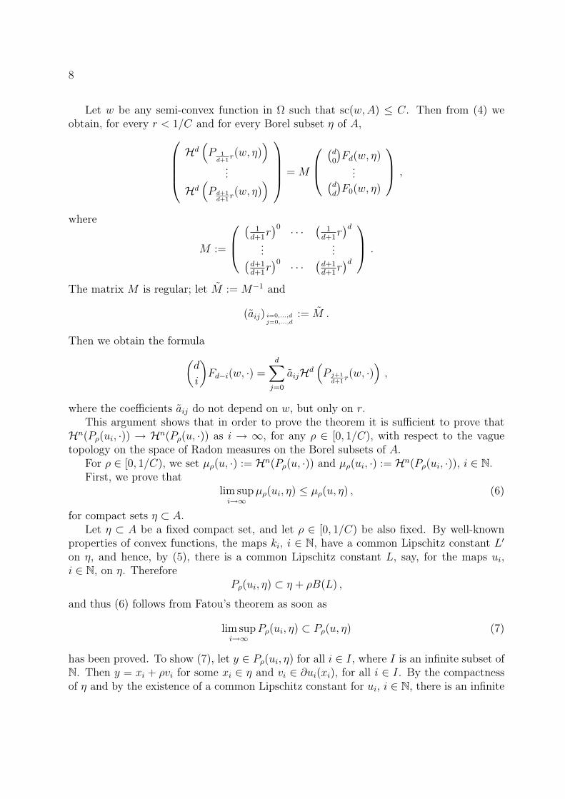
Let w be any semi-convex function in Ω such that sc(w,A) ≤ C. Then from (4) weobtain, for every r < 1/C and for every Borel subset η of A,

Hd(P 1

d+1r(w, η)

)...

Hd(P d+1

d+1r(w, η)

) = M

(

d0

)Fd(w, η)

...(dd

)F0(w, η)

,

where

M :=

(

1d+1

r)0 · · ·

(1

d+1r)d

......(

d+1d+1

r)0 · · ·

(d+1d+1

r)d

.

The matrix M is regular; let M := M−1 and

(aij) i=0,...,dj=0,...,d

:= M .

Then we obtain the formula(d

i

)Fd−i(w, ·) =

d∑j=0

aijHd(P j+1

d+1r(w, ·)

),

where the coefficients aij do not depend on w, but only on r.This argument shows that in order to prove the theorem it is sufficient to prove that

Hn(Pρ(ui, ·)) → Hn(Pρ(u, ·)) as i → ∞, for any ρ ∈ [0, 1/C), with respect to the vaguetopology on the space of Radon measures on the Borel subsets of A.

For ρ ∈ [0, 1/C), we set µρ(u, ·) := Hn(Pρ(u, ·)) and µρ(ui, ·) := Hn(Pρ(ui, ·)), i ∈ N.First, we prove that

lim supi→∞

µρ(ui, η) ≤ µρ(u, η) , (6)

for compact sets η ⊂ A.Let η ⊂ A be a fixed compact set, and let ρ ∈ [0, 1/C) be also fixed. By well-known

properties of convex functions, the maps ki, i ∈ N, have a common Lipschitz constant L′

on η, and hence, by (5), there is a common Lipschitz constant L, say, for the maps ui,i ∈ N, on η. Therefore

Pρ(ui, η) ⊂ η + ρB(L) ,

and thus (6) follows from Fatou’s theorem as soon as

lim supi→∞

Pρ(ui, η) ⊂ Pρ(u, η) (7)

has been proved. To show (7), let y ∈ Pρ(ui, η) for all i ∈ I, where I is an infinite subset ofN. Then y = xi + ρvi for some xi ∈ η and vi ∈ ∂ui(xi), for all i ∈ I. By the compactnessof η and by the existence of a common Lipschitz constant for ui, i ∈ N, there is an infinite

9

subset J ⊂ I such that xi → x ∈ η and vi → v as i → ∞ and i ∈ J . By (5) and thecharacterization of subgradients in (2), it follows that v ∈ ∂u(x), and hence y = x + ρv,where x ∈ η and v ∈ ∂u(x). Thus (7) is established.

Next we show that

lim infi→∞

µρ(ui, η) ≥ µρ(u, η) ,

for all open sets η ⊂ A whose closure is a compact subset of A. Let such a set η be fixed.By Fatou’s theorem it is sufficient to show that

Pρ(u, η) ⊂ lim infi→∞

Pρ(ui, η) . (8)

Let y ∈ Pρ(u, η). Then y = x + ρv − ρCx, where x ∈ η and v ∈ ∂k(x), and hencey′ := x + ρv ∈ Pρ(k, η). Now we apply Lemma 1.4 to the sequence of convex functions ki,i ∈ N, k, and an open, convex and bounded neighbourhood of A in Ω. Using the notationof this lemma, we can write:

y′ ∈ Pρ(w, η) ⊂ η + ρB(L) ⊂ B(R/2) + B(ρL) ⊂ B(R + ρL) .

Since ρ, R are fixed, there is some i0 ∈ N such that

Pρ(w, η) ⊂ B(2R + ρLi) = Pρ(wi, B(2R)) ,

for i ≥ i0. Here parts (iii) and (iv) of Lemma 1.4 were used. Therefore we can findxi ∈ B(2R) and vi ∈ ∂wi(xi) such that y′ = xi +ρvi. Using the compactness of B(2R), thefact that the sequence lip(wi, A) is bounded and Theorem VI.6.2.7 in [30], we may assumethat the sequences xi, vi, i ∈ N, converge to x0 ∈ B(2R) and to v ∈ ∂w(x0), respectively;hence y′ = x0 + ρv0. On the other hand, y′ = x + ρv with x ∈ η and v ∈ ∂k(x) = ∂w(x).The uniqueness of this decomposition (with respect to w) yields that x0 = x ∈ η. Recallthat η is open. Hence, for i ≥ i1(≥ i0) we obtain that xi ∈ η, and thus y′ = xi +ρvi, xi ∈ η,vi ∈ ∂wi(xi) = ∂ki(xi). This demonstrates that y′ ∈ Pρ(ki, η), and then y ∈ Pρ(ui, η), fori ≥ i1, that is

y ∈ lim infi→∞

Pρ(ui, η) .

This yields (8) and thus completes the proof. 2

Lemma 1.5 Let Ω be an open subset of Rd, let u : Ω → R be a semi-convex function, andlet Ω′ ⊂⊂ Ω. Then there exists a sequence of C∞ functions ui : Ω → R, i ∈ N, such that

(a) ui → u pointwise on Ω′ as i →∞;

(b) lip(ui, Ω′), sc(ui, Ω

′), i ∈ N, are bounded sequences;

(c) Fk(ui, ·) → Fk(u, ·) on Ω′ in the vague topology as i →∞, for k ∈ 0, 1, . . . , d.

10

Proof. Choose Ω′′ ⊂⊂ Ω such that Ω′ ⊂⊂ Ω′′. Then there exists a convex functionk : Ω′′ → R and a constant C ≥ 0 with

u(x) = k(x)− C

2‖x‖2, x ∈ Ω′′ .

Lemma 2.3 in [13] applied to k|Ω′ shows that there is a convex and Lipschitz functionk : Rd → R such that k|Ω′ = k. By Lemma 2.4 in [13] we obtain a sequence of convex C∞

functions ki : Rd → R, i ∈ N, which satisfy ki(x) → k(x) = k(x) for all x ∈ Ω′. Now wedefine

ui(x) := ki(x)− C

2‖x‖2, x ∈ Ω .

Then ui is of class C∞ and (a) is fulfilled. Moreover, (b) is implied by the properties of ki

and the relative compactness of Ω′. Finally, (c) follows from Theorem 1.1. 2

Proposition 1.6 Let Ω be an open subset of Rd, and let u : Ω → R be semi-convex.Further, let C ∈ R and let the semi-convex function v : Ω → R be defined by

v(x) := u(x) +C

2‖x‖2 , x ∈ Ω .

Then, for k ∈ 0, 1, . . . , d and for relatively compact, Borel measurable subsets η of Ω,

Fk(u, η) =d−k∑j=0

(d− k

j

)(−C)jFk+j(v, η) . (9)

Proof. From the expression of Hessian measures for smooth functions (see (3)) it followsimmediately that (9) is true for every u ∈ C2(Ω). Then the conclusion follows immediatelyfrom the preceding Lemma 1.5. 2

Remark 1.2 Proposition 1.6 is particularly useful when v is a convex function. Since forany semi-convex function this can be assumed locally, equation (9) can be used for prov-ing assertions about semi-convex functions by verifying corresponding results for convexfunctions only.

Remark 1.3 In the papers [41] and [42] N. Trudinger and X. J. Wang proved the existenceof the first k Hessian measures in the class of k-convex functions. Roughly speaking afunction u defined in an open subset Ω of Rd is k-convex, for some k ∈ 0, 1, . . . , d, if itcan be approximated pointwise by a decreasing sequence of functions ui ∈ C2(Ω), i ∈ N,such that Sj(D

2ui(x)) ≥ 0 for every j ∈ 0, 1, . . . , k, i ∈ N, and x ∈ Ω. We notice thatd-convexity is equivalent to the usual convexity.

Furthermore, in [42, Section 4] the notion of Hessian measures is extended to theclass of k-semi-convex functions, i.e. the functions of the form u(x) − C/2‖x‖2, where

11

u is k-convex and C ≥ 0 is a constant. Such an extension is performed as follows: ifv(x) = u(x) − C/2‖x‖2, where u is k-convex and C ≥ 0, then the k-th Hessian measureFk(v, ·) of v is defined through the Hessian measures of u by the formula

Fk(v, ·) :=k∑

j=0

(d− k

j

)(−C)jFk+j(u, ·) .

Thus, in particular, the definition of Hessian measures by Trudinger and Wang is givenin a class which includes semi-convex functions; we notice that such a definition coincideswith the one given in the present paper. (It should be observed that our measures

(dk

)Fd−k

correspond to the measures Fk in the notation of Trudinger and Wang.) Indeed by theabove formula and by a special case of Proposition 1.6 it is enough to prove the equivalenceof the two definitions in the class of convex functions. On the other hand in this class suchan equivalence is straightforward since

1. the two definitions coincide for smooth convex functions;

2. both definitions require convergence of Hessian measures with respect to the vaguetopology, for approximating sequences of smooth convex functions.

2 A Crofton formula for semi-convex functions

We denote by SO(d) the topological group of proper rotations of Rd, and by ν the Haarprobability measure on SO(d). For every d ≥ 1 and k ∈ 0, 1, . . . , d, let A(d, k) be thefamily of all k-dimensional affine subspaces of Rd; following [36, §4.5] we construct aninvariant measure µk over A(d, k). Let E0 be a fixed k-dimensional linear subspace, anddenote by E⊥

0 its orthogonal complement in Rd. Consider the surjective map

γk : E⊥0 × SO(d) → A(d, k) , γ(t, ρ) := ρ(E0 + t) .

The set A(d, k) is endowed with the finest topology such that γk is continuous. Then themeasure µk is defined as the image measure of the product measure λd−k ⊗ ν under γk,defined on the Borel subsets of E⊥

0 × SO(d), where λd−k is the restriction of Hd−k to theBorel subsets of E⊥

0 . Thus µk is a Radon measure on the Borel sets of A(d, k).Let Ω be an open subset of Rd, and let u : Ω → R be a semi-convex function. For

k ∈ 0, 1, . . . , d and E ∈ A(d, k), we denote by u|Ω∩E the restriction of u to Ω ∩ E. Thefunction u|Ω∩E is semi-convex on Ω∩E, hence its Hessian measures are defined; we denote

them by F(k)j (u|Ω∩E, ·), j ∈ 0, 1, . . . , k.

In this section we will prove the following:

Theorem 2.1 Let Ω be an open subset of Rd, and let u : Ω → R be a semi-convexfunction. Further, let k ∈ 1, 2, . . . , d, j ∈ 0, 1, . . . , k, and let η be a relatively compact,Borel measurable subset of Ω. Then

Fd+j−k(u, η) =

∫A(d,k)

F(k)j (u|Ω∩E, η ∩ E)dµk(E) .

12

In order to prove this theorem, we need two lemmas.

Lemma 2.2 Let Ω be an open subset of Rd, and let u : Ω → R be semi-convex. If η is arelatively compact, Borel measurable subset of Ω, then the function

gη : A(d, k) → R , gη(E) := F(k)j (u|Ω∩E, η ∩ E) ,

is Borel measurable.

Proof. Let Ω′ ⊂⊂ Ω be arbitrarily chosen. Using the argument described in the be-ginning of the proof of Theorem 1.1, we see that it is sufficient to prove that for everyρ ∈ [0, sc(u, Ω′)−1) and for every Borel subset η of Ω′ the function

Gη : A(d, k) → R , Gη(E) := Hk(P (E)ρ (u|Ω∩E, η ∩ E)) ,

is Borel measurable, where

P (E)ρ (u|Ω∩E, η ∩ E) := x + ρv : x ∈ η ∩ E, v ∈ ∂(u|Ω∩E) .

Notice that the function Gη is nonnegative.Let ρ ∈ [0, sc(u, Ω′)−1) be fixed and let η be a compact subset of Ω′. Since u is Lipschitz

on Ω′ and Gη remains unchanged if u is modified in the complement of Ω′, we can assumethat u is defined and semi-convex on Rd (see Lemma 2.3 in [13]).

Let E, Ei ∈ A(d, k), i ∈ N, be such that Ei → E as i → ∞. Then we can find(t, σ), (ti, σi) ∈ E⊥

0 × SO(d), i ∈ N, such that E = γk(t, σ), Ei = γk(ti, σi), for i ∈ N, and(ti, σi) → (t, σ) as i → ∞. For every i ∈ N, consider the isometry ζi : E → Ei which isgiven by

ζi(x) = σi(σ−1(x)− t + ti) , x ∈ E ,

and the functionvi = u|Ei

ζi = u ζi ,

which is defined on E. Since ζi(x) → x as i →∞ for all x ∈ E and since u is continuous,we obtain that vi → u pointwise on E as i → ∞. Moreover, for any U ⊂⊂ E there issome U∗ ⊂⊂ Rd such that ζi(U) ⊂ U∗ for all i ∈ N. This implies that sc(vi, U) ≤ sc(u, U∗)for all i ∈ N. Therefore the sequence sc(vi, U), i ∈ N, is bounded for any U ⊂⊂ E andvi is semi-convex for all i ∈ N. Hence Theorem 1.1 can be applied and we deduce thatthe sequence of measures Hk(P

(E)ρ (vi|Ω′∩E, ·)), i ∈ N, converges in the vague topology to

Hk(P(E)ρ (u|Ω′∩E, ·)).

Set ηi := ζ−1i (η ∩ Ei) and η := η ∩ E. We have that

P (Ei)ρ (u|Ei

, η ∩ Ei) = ζi(P(E)ρ (vi, ηi)) ,

and henceHk(P (Ei)

ρ (u|Ei, η ∩ Ei)) = Hk(P (E)

ρ (vi, ηi)) ,

13

for all i ∈ N. The sets ηi, i ∈ N, are compact subsets of E. For ε > 0 we set

ηε := x ∈ E : dist(x, η) ≤ ε .

If ε > 0 is sufficiently small, then ηε ⊂ Ω′ ∩E; fix any such ε > 0 for the moment. If i ∈ Nis sufficiently large, then ηi ⊂ ηε. Therefore

Hk(P (E)ρ (u|E, ηε)) ≥ lim sup

i→∞Hk(P (E)

ρ (vi, ηε))

≥ lim supi→∞

Hk(P (E)ρ (vi, ηi)) (10)

= lim supi→∞

Hk(P (Ei)ρ (u|Ei

, η ∩ Ei)) .

On the other hand,

Hk(P (E)ρ (u|E, η ∩ E)) = inf

ε>0Hk(P (E)

ρ (u|E, ηε)) . (11)

To see this, note that u|E is Lipschitz in ηε for ε small enough, so that the set P(E)ρ (u|E, ηε)

is bounded.From (10) and (11) it follows that the function Gη is upper semi-continuous, and hence

measurable, whenever η is a compact subset of Ω′.Let G be the class of all sets η ⊂ Ω′ for which Gη is Borel measurable. Obviously, G

is a Dynkin system (see [6]) which contains the closed subsets of Ω′. Therefore G containsthe Borel subsets of Ω′. But this immediately implies the assertion of the lemma. 2

If u ∈ C2(Ω), where Ω is an open subset of Rd, and v1, v2, . . . , vk is any basis of thelinear subspace parallel to E ∈ A(d, k), then the Hessian matrix of u|Ω∩E at x ∈ Ω ∩ E,with respect to the chosen basis, is given by

D2(u|Ω∩E)(x) =(〈D2u(x)vi, vj〉

)i,j=1,2,...,k

.

Lemma 2.3 Let Ω be an open subset of Rd, u ∈ C2(Ω), k ∈ 1, 2, . . . , d, and j ∈0, 1, . . . , k. Then∫

A(d,k)

∫η∩E

Sj(D2(u|Ω∩E)(x))dHk(x)dµk(E) = βdjk

∫η

Sj(D2u(x))dHd(x) ,

where βdjk =(

dk

)−1(d−jk−j

).

Proof. Let E0 be a k-dimensional linear subspace in Rd, and let E⊥0 be the orthogonal

complement of E0 in Rd. Taking into account the definition of the measure µk, we canwrite ∫

A(d,k)

∫η∩E

Sj(D2(u|Ω∩E)(x))dHk(x)dµk(E) (12)

=

∫SO(d)

∫E⊥0

∫η∩ρ(E0+t)

Sj(D2(u|Ω∩ρ(E0+t))(x))dHk(x)dHd−k(t)dν(ρ) .

14

Now let vr : r = 1, 2, . . . , k be an orthonormal basis of E0; for every ρ ∈ SO(d),ρ(vr) : r = 1, 2, . . . , k is an orthonormal basis of ρ(E0). Hence

Sj(D2(u|Ω∩ρ(E0+t))(x)) = Sj

[(〈D2u(x)ρ(vi), ρ(vj)〉

)i,j=1,2,...,k

], (13)

for any t ∈ E⊥0 and x ∈ Ω ∩ ρ(E0 + t). Substituting (13) into (12) and using Fubini’s

theorem, we obtain∫A(d,k)

∫η∩E

Sj(D2(u|Ω∩E)(x))dHk(x)dµk(E)

=

∫SO(d)

∫η

Sj

[(〈D2u(x)ρ(vi), ρ(vj)〉

)i,j=1,2,...,k

]dHd(x)dν(ρ) .

The left-hand side of the preceding formula is independent of the choice of E0. Letv1, v2, . . . , vd be an orthonormal basis of Rd. Fix k indices i1, i2, . . . , ik ∈ 1, 2, . . . , dso that 1 ≤ i1 < i2 < · · · < ik ≤ d, and let E0 be the linear subspace spannedby vi1 , vi2 , . . . , vik . Then, repeating the above argument for every choice of the indicesi1, i2, . . . , ik ∈ 1, 2, . . . , d, and summing over all possible choices, we obtain(

d

k

) ∫A(d,k)

∫η∩E

Sj(D2(u|Ω∩E)(x))dHk(x)dµk(E) (14)

=

∫SO(d)

∫η

∑|I|=k

Sj

[(〈D2u(x)ρ(vr), ρ(vs)〉

)r,s∈I

]dHd(x)dν(ρ) ,

where the summation is extended over all subsets I ⊂ 1, . . . , d of cardinality k. On theother hand, it is readily seen that∑

|I|=k

Sj

[(〈D2u(x)ρ(vr), ρ(vs)〉

)r,s∈I

]=

(d− j

k − j

)Sj(D

2u(x)) . (15)

To complete the proof, it is sufficient to insert (15) into (14). 2

Proof of Theorem 2.1. It is sufficient to consider the case where Ω′ ⊂⊂ Ω and η is aBorel measurable subset of Ω′.

Step 1. Assume that u ∈ C2(Ω), fix a Borel subset η of Ω′, k ∈ 1, 2, . . . , d andj ∈ 0, 1, . . . , k. By (3) and the previous lemma, we obtain(

k

j

)(d

k

)Fd+j−k(u, η) =

(d− k + j

j

) ∫η

Sk−j(D2u(x))dHd(x)

=

(d

k

) ∫A(d,k)

∫η∩E

Sk−j(D2(u|Ω∩E)(x))dHk(x)dµk(E)

=

(k

j

)(d

k

) ∫A(d,k)

F(k)j (u|Ω∩E, η ∩ E)dµk(E) .

15

Hence it follows that the theorem is true for C2 functions. Moreover, for any continuousfunction f : Rd → R with compact support contained in Ω′, we deduce∫

Ω

f(x)dFd+j−k(u, x) =

∫A(d,k)

∫Ω∩E

f(x)dF(k)j (u|Ω∩E, x)dµk(E) . (16)

In order to prove the theorem, we have to show that (16) is true for an arbitrary semi-convexfunction u on Ω.

Step 2. By Lemma 1.5 there exists a sequence of semi-convex functions ui : Ω → R,ui ∈ C∞(Ω), i ∈ N, converging pointwise to u on Ω′ and such that

lip(ui, Ω′), sc(ui, Ω

′) ≤ C , (17)

for some positive constant C and for all i ∈ N.

Let f : Rd → R be a continuous function with compact support contained Ω′. Theorem1.1 yields

limi→∞

∫Ω′

f(x)dFd+j−k(ui, x) =

∫Ω′

f(x)dFd+j−k(u, x) . (18)

Furthermore, for every E ∈ A(d, k) the sequence ui|Ω′∩E, i ∈ N, converges pointwise tou|Ω′∩E, and by (17) the sequence sc(ui|Ω′∩E, Ω′∩E), i ∈ N, is bounded. Another applicationof Theorem 1.1 thus yields

limi→∞

∫Ω′∩E

f(x)dF(k)j (ui|Ω′∩E, x) =

∫Ω′∩E

f(x)dF(k)j (u|Ω′∩E, x) ,

for every E ∈ A(d, k).

Now taking into account that the functions ui are uniformly Lipschitz in Ω′ (by (17)),that Ω′ is bounded, and using Proposition 1.6 of the present paper and Theorem 6.2 in[14], it is possible to prove that there exists a constant K > 0, depending on C, diam(Ω′),k and d, such that ∫

Ω′∩E

f(x)dF(k)j (ui|Ω′∩E, x) ≤ K‖f‖∞ ,

for every i ∈ N and for every E ∈ A(d, k). Hence we can apply the dominated convergencetheorem to obtain

limi→∞

∫A(d,k)

∫Ω′∩E

f(x)dF(k)j (ui|Ω′∩E, x)dµk(E) (19)

=

∫A(d,k)

∫Ω′∩E

f(x)dF(k)j (u|Ω′∩E, x)dµk(E) .

The proof can now be completed by combining (18), (19) and the result of step 1. 2

16

3 Absolute continuity of Hessian measures

In this section we study the absolute continuity of the k-th Hessian measure of a semi-convex function with respect to the k-dimensional Hausdorff measure Hk. Recall that fortwo Borel measures µ, ν over Rd one defines that µ is absolutely continuous with respectto ν if ν(A) = 0 implies µ(A) = 0 for all Borel sets A ⊂ Rd. If this is the case and ifthe restriction νxB of ν to a fixed Borel set B ⊂ Rd is σ-finite, then it follows by theabstract Radon-Nikodym theorem of measure theory that µxB has a density with respectto νxB. The explicit determination of this density in the present framework is the subjectof Section 4.

We wish to emphasize already at this point that the results and remarks of this sectionalmost immediately lead to corresponding results for curvature and surface area measures,as soon as the results of Section 5 are available.

The crucial result in this section is the following theorem; its proof is based on an ideawhich was applied in the context of curvature measures by H. Fallert [16].

Theorem 3.1 Let Ω be an open subset of Rd, and let u : Ω → R be a semi-convexfunction. Then, for every k ∈ 0, 1, . . . , d, the k-th Hessian measure of u, Fk(u, ·), isabsolutely continuous with respect to Hk over Ω.

Proof. A decomposition argument shows that it is sufficient to consider Borel subsets ηof a set Ω′ ⊂⊂ Ω. Moreover, by virtue of Proposition 1.6, it suffices to prove the theoremin the special case where u is convex in Ω′.

We denote by Θj(u, ·), j ∈ 0, 1, . . . , d the support measures whose existence is provedin [14, Theorem 3.1]. We recall that Θj(u, ·), for every j ∈ 0, 1, . . . , d, is a nonnegativeBorel measure over Ω′ × Rd and

Fj(u, η) = Θj(u, η × Rd) , (20)

for every Borel subset η of Ω′.Let i ∈ 0, 1, . . . , d and let η ⊂ Ω′ be a Borel set which satisfies Hd−i(η) = 0. From

(20) it follows that it is sufficient to prove that Θd−i(u, η×B(L)) = 0 for every L > 0. Letz ∈ Rd and r > 0 be arbitrarily chosen. We write B(z, r) for the ball of radius r centredat z. Fix an arbitrary L > 0. Taking into account the defining relation for the measuresΘj(u, ·) (see [14, Theorem 3.1]), we may argue as in the beginning of the proof of Theorem1.1 and thus obtain(

d

i

)Θd−i(u, (B(z, r) ∩ η)×B(L)) =

d∑j=0

aijHd(P j+1

d+1r(u, (B(z, r) ∩ η)×B(L))

), (21)

where the coefficients aij are such that the matrix

M := (aij) i=0,...,dj=0,...,d

17

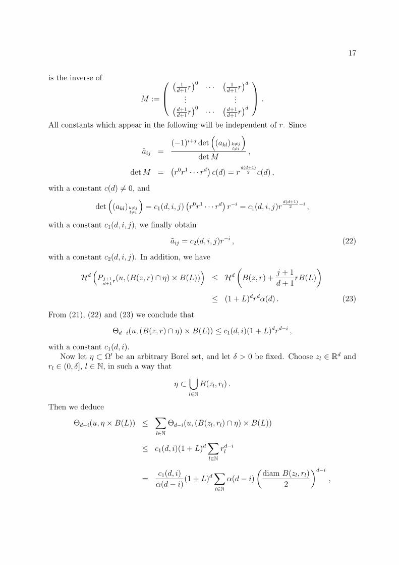
is the inverse of

M :=

(

1d+1

r)0 · · ·

(1

d+1r)d

......(

d+1d+1

r)0 · · ·

(d+1d+1

r)d

.

All constants which appear in the following will be independent of r. Since

aij =(−1)i+j det

((akl) k 6=j

l6=i

)det M

,

det M =(r0r1 · · · rd

)c(d) = r

d(d+1)2 c(d) ,

with a constant c(d) 6= 0, and

det((akl) k 6=j

l6=i

)= c1(d, i, j)

(r0r1 · · · rd

)r−i = c1(d, i, j)r

d(d+1)2

−i ,

with a constant c1(d, i, j), we finally obtain

aij = c2(d, i, j)r−i , (22)

with a constant c2(d, i, j). In addition, we have

Hd(P j+1

d+1r(u, (B(z, r) ∩ η)×B(L))

)≤ Hd

(B(z, r) +

j + 1

d + 1rB(L)

)≤ (1 + L)drdα(d) . (23)

From (21), (22) and (23) we conclude that

Θd−i(u, (B(z, r) ∩ η)×B(L)) ≤ c1(d, i)(1 + L)drd−i ,

with a constant c1(d, i).Now let η ⊂ Ω′ be an arbitrary Borel set, and let δ > 0 be fixed. Choose zl ∈ Rd and

rl ∈ (0, δ], l ∈ N, in such a way that

η ⊂⋃l∈N

B(zl, rl) .

Then we deduce

Θd−i(u, η ×B(L)) ≤∑l∈N

Θd−i(u, (B(zl, rl) ∩ η)×B(L))

≤ c1(d, i)(1 + L)d∑l∈N

rd−il

=c1(d, i)

α(d− i)(1 + L)d

∑l∈N

α(d− i)

(diam B(zl, rl)

2

)d−i

,

18

and hence

Θd−i(u, η ×B(L)) ≤ c2(d, i)(1 + L)d Sd−iδ (η)

≤ c2(d, i)(1 + L)d Sd−i(η)

≤ c2(d, i)(1 + L)d2d−iHd−i(η) = 0 ,

where c2(d, i) is a constant and Sd−i denotes the (d− i)-dimensional spherical measure overRd (see [18], Section 2.10.2). This yields the desired conclusion. 2

Remark 3.1 The construction of Hessian measures, which was carried out for finite convexfunctions in [14], immediately extends to (proper) closed convex functions defined on Rd

which take values in R (confer Section 5). Furthermore for such functions the same proofas in the above theorem can be repeated. Hence if u : Rd → R is closed and convex, thenthe j-th Hessian measure Fj(u, ·) of u is absolutely continuous with respect to Hj in Rd,for every j ∈ 0, 1, . . . , d.

Remark 3.2 For convex Lipschitz functions which take values in R a more precise resultthan Theorem 3.1 can be proved by a different approach. Let Ω be an open convex subsetof Rd, let u : Ω → R be a convex Lipschitz function with Lipschitz constant L, and letj ∈ 0, 1, . . . , d. Then

Fj(u, ·) ≤ c(d, j)Ld−j Hj ,

where c(d, j) =(

2dd+1

) j2 α(d)

α(j). This fact can be proved as follows. Let z ∈ Rd and r ≥ 0 be

such that B(z, r) ⊂ Ω. Then Theorem 6.2 in [14] yields

Fj(u, B(z, r)) ≤ Ld−jWd−j(B(z, r)) = Ld−jrjα(d) ,

where the quantities Wj(B(z, r)), j ∈ 0, 1, . . . , d, denote the quermassintegrals of B(z, r).The remaining part of the proof is a repetition of the proof for Theorem 3.1.

4 Radon-Nikodym derivatives of Hessian measures

Let Ω be an open convex subset of Rd and let u : Ω → R be semi-convex. In the previoussection we have seen that the j-th Hessian measure Fj(u, ·) of u is absolutely continuouswith respect to the measure Hj, for every j ∈ 0, 1, . . . , d. In the present section wecompute the Radon-Nikodym derivative of Fj(u, ·) with respect to Hj on subsets of Ω ofσ-finite j-dimensional Hausdorff measure. Thus we obtain a generalization of Theorem 5.3in [14], since the set Σj(u), j ∈ 0, 1, . . . , d, of j-singular points of u (see the definition inthe proof of Theorem 4.2) is countably j-rectifiable and hence has σ-finite j-dimensionalHausdorff measure.

In order to determine the Radon-Nikodym derivative we need a lemma.

19

Lemma 4.1 Let Ω ⊂ Rd be open, x ∈ Ω, let u : Ω → R be semi-convex, and let x ∈ E ∈A(d, d− j) for some j ∈ 0, 1, . . . , d− 1. Then

dim ∂(u|Ω∩E)(x) ≤ dim ∂u(x) .

Proof. Equation (1) shows that it is sufficient to prove the assertion for convex functions.Furthermore, by the interplay between convex functions and their epigraphs, the assertionfollows from the following geometric statement. Let K ⊂ Rd be a closed convex set, letE ∈ A(d, k) for some k ∈ 1, . . . , d, and assume that E ∩ int K 6= ∅. Let L(E) denote thelinear subspace parallel to E, and let x ∈ E ∩ ∂K. Then

NE(K ∩ E, x) = N(K, x)|L(E) ,

where NE(K ∩ E, x) is the normal cone of K ∩ E at x taken in E and N(K, x)|L(E) isthe orthogonal projection of the normal cone of K at x onto L(E). Further, let S(K, x)denote the support cone of K at x and let SE(K ∩E, x) denote the support cone of K ∩Eat x (calculated in E). Using notation and results as described in Section 2.2 of [36], weobtain

NE(K ∩ E, x) = (SE(K ∩ E, x))∗ = (S(K, x) ∩ L(E))∗ = S(K, x)∗|L(E)

= N(K, x)|L(E) ,

where the first and the second formation of polar cones is taken in L(E). 2

Theorem 4.2 Let Ω be an open subset of Rd, and let u : Ω → R be semi-convex. Letj ∈ 0, 1, . . . , d, and let Γ ⊂ Ω be a Borel set having σ-finite j-dimensional Hausdorffmeasure. Then (

d

j

)Fj(u, Γ) =

∫Γ

Hd−j(∂u(x))dHj(x) . (24)

Proof. For the proof we can assume that Ω′ ⊂⊂ Ω and Γ ⊂ Ω′ has finite j-dimensionalHausdorff measure.

For k ∈ 0, 1, . . . , d we define the set of singular points of order k of u by

Σk(u) := x ∈ Ω : dim(∂u(x)) ≥ d− k .

In [14, Theorem 5.3] it is proved that(d

j

)Fj(u, Γ ∩ Σj(u)) =

∫Γ∩Σj(u)

Hd−j(∂u(x))dHj(x) ,

and hence, by the definition of Σj(u),(d

j

)Fj(u, Γ ∩ Σj(u)) =

∫Γ

Hd−j(∂u(x))dHj(x) .

20

It remains to prove that Fj(u, Γ \ Σj(u)) = 0.

By [18, Section 3.2.14] Γ can be split into two disjoint Borel sets, Γ = Γr ∪ Γu, whereΓr is countably j-rectifiable, and Γu is purely (Hj, j)-unrectifiable. Set Γj

r := Γr \ Σj(u)and Γj

u := Γu \ Σj(u).

Let us prove that

Fj(u, Γjr) = 0 . (25)

A special case of Theorem 2.1 yields

Fj(u, Γjr) =

∫A(d,d−j)

F(d−j)0 (u|Ω∩E, Γj

r ∩ E)dµd−j(E) . (26)

Since Γjr is (Hj, j)-rectifiable, Theorem 3.3.13 and Section 2.10.16 in [18] yield, for µd−j

almost every E ∈ A(d, d− j), that E ∩ Γjr is a finite set. Hence

Fj(u, Γjr) =

∫A′

F(d−j)0 (u|Ω∩E, Γj

r ∩ E)dµd−j(E) , (27)

where A′ is the set of all E ∈ A(d, d− j) for which Γjr ∩ E is non-empty and finite.

Now let E ∈ A′, and Γjr ∩ E = x1, x2, . . . , xp. Since dim(∂u(xi)) < d − j for all

i ∈ 1, . . . , p, and since F(d−j)0 (u|Ω∩E, xi) is the (d − j)-dimensional measure of the

image set of xi through the subgradient of u|Ω∩E (see [13, Theorem 5.3]), Lemma 4.1implies

F(d−j)0 (u|Ω∩E, xi) = 0 , i = 1, 2, . . . , p ,

and then

F(d−j)0 (u|Ω∩E, Γj

r ∩ E) = 0 . (28)

Using (28), which holds for every E ∈ A′, and (27), we get (25).

Now using again formula (26) with Γjr replaced by Γj

u, and [18, Theorem 3.3.13 andSection 2.10.16], we obtain that

Fj(u, Γju) = 0 ,

which completes the proof. 2

Remark 4.1 It is a remarkable consequence of Theorem 4.2 that the restriction of thesigned Hessian measure Fj(u, ·) of a semi-convex function u to sets having σ-finite j-dimensional Hausdorff measure yields a nonnegative measure. Moreover, the proof of thepreceding theorem shows that Theorem 5.3 in [14] can be generalized in the same way. Thisfact will be used in the following section. We finally remark that in view of Proposition1.6 it would be sufficient to prove Theorem 4.2 for convex functions.

21

5 Applications to support measures

In this section we shall explain the basic relationship between Hessian measures of semi-convex functions and support measures of sets of positive reach. In [14], the epigraph ofa semi-convex function (which is a set of positive reach) was used in a non-trivial wayto construct the Hessian measures of the given function. Now we shall see that supportmeasures of a set with positive reach can be expressed in a simple way as Hessian measuresof some particular functions related to the given set, such as the distance function, supportfunction and convex characteristic function.

Before we go into the details of the results, we recall some basic notions and introducesome notations regarding sets of positive reach and convex bodies in Rd. For a subset Xof Rd and for r ≥ 0 we denote by Xr the set of points whose distance from X is r at themost. The reach of X, reach(X), is the supremum over all r ≥ 0 such that for every pointx ∈ Xr there exists a unique nearest point in X to x. We say that X ⊂ Rd is a set ofpositive reach (has positive reach) if reach(X) > 0.

A convex body K in Rd, i.e. a convex compact subset of Rd with non-empty interior, isclearly a set of positive reach and reach(K) = ∞.

Let X ⊂ Rd have positive reach; for r < reach(X) and x ∈ Xr \X we write p(X, x) forthe nearest point in X to x, and we set u(X, x) := dX(x)−1(x − p(X, x)), where dX(x) isthe distance of x to X. Furthermore for every x ∈ X, we denote by N(X, x) the normalcone of X at x (see [17]); the definition given there is consistent with the one adopted inconvex geometry. Also recall that if X is a convex body and u ∈ Sd−1, then

F (X, u) := x ∈ X : u ∈ N(X, x)

is the support set of X in direction u.The support measures Θj(X, ·), j = 0, 1, . . . , d−1, of a set X ⊂ Rd of positive reach are

signed measures defined for all bounded Borel subsets of Rd×Sd−1. They can be obtainedas coefficients of the local Steiner formula

Hd(Mr(X, η)) =1

d

d−1∑j=1

rd−j

(d

r

)Θj(X, η) ,

where 0 < r < reach(X), η is a bounded Borel subset of Rd × Sd−1 and

Mr(X, η) := x ∈ Xr \X : (p(X, x), u(X, x)) ∈ η .

By specializing η we obtain the Federer curvature measures (briefly: curvature measures)of X as follows

Cj(X, α) := Θj(X, α× Sd−1) , j ∈ 0, 1, . . . , d− 1 ,

for every bounded Borel set α ⊂ Rd. Moreover in the special case where X = K is a convexbody we can also introduce the surface area measures of K by setting

Sj(K, β) := Θj(K, Rd × β) , j ∈ 0, 1, . . . , d− 1 ,

22

for every Borel subset β of Sd−1.Now we are in the position to show some applications of the results proved in the

previuos sections to support measures of sets of positive reach. We start with a preliminarylemma which shows that we could have chosen a seemingly weaker definition of semi-convexity in the first instance. We include this simple lemma, because the method of proofwill also be useful in the following.

Lemma 5.1 Let Ω ⊂ Rd be open, and let u : Ω → R be a function. Then u is semi-convexif and only if for each x ∈ Ω there exists a neighbourhood U ⊂⊂ Ω of x and a constantC ≥ 0 such that

k(x) := u(x) +C

2‖x‖2 , x ∈ U ,

defines a convex function.

Proof. We prove the “if part”. Let Ω′ ⊂⊂ Ω be given. Then there are neighbourhoodsU1, . . . , Up ⊂ Ω and constants C1, . . . , Cp ≥ 0 such that

ki(x) := u(x) +Ci

2‖x‖2 , x ∈ Ui ,

for i = 1, . . . , p, defines a convex function. We set

C := maxCi : 1 ≤ i ≤ p

and

k(x) := u(x) +C

2‖x‖2, x ∈ Ω′ .

Obviously, k|Uiis a convex function for each i ∈ 1, . . . , p, and therefore the epigraph of

each of these functions is an open convex set. But then the epigraph of k|Ω′ fulfills thelocal support property which is required for an application of Tietze’s convexity criterion;see [43], Theorem 4.10. Thus k|Ω′ is a convex function. 2

In the more general context of Riemannian geometry, a less explicit version of thefollowing proposition has been proved by Kleinjohann [33], Satz 2.8; see also [8] and [19],Corollary 3.4, for a converse.

Proposition 5.2 Let X ⊂ Rd satisfy reach(X) > r > 0 and let 0 < δ < r. Then dX issemi-convex on int Xr−δ; in particular, sc(dX , Ω′) ≤ δ−1 for all Ω′ ⊂⊂ int Xr−δ.

Proof. We show that

k(x) := dX(x) +1

2δ‖x‖2 , x ∈ Rd ,

defines a convex function on convex subsets of int Xr−δ. In view of the proof of Lemma 5.1we have to show that for each x0 ∈ int Xr−δ there is some r0 > 0 such that the epigraphof k|B(x0,r0) is supported by a hyperplane at (x0, k(x0)).

23

If x0 ∈ X, then the support property is satisfied since dX ≥ 0 and x 7→ (2δ)−1‖x‖2

is convex. Now let x0 ∈ (int Xr−δ) \ X. We define p0 := p(X, x0), u0 := u(X, x0) andr0 := 2−1 mindX(x0), r − δ − dX(x0), and hence we obtain

B(x0, r0) ⊂ B(p0 + ru0, r) \B(p0 + ru0, δ) .

Furthermore, we define C := Rd \ int B(p0 + ru0, r); a straightforward calculation thenshows that

x 7→ dC(x) +1

2δ‖x‖2

defines a convex function on B(x0, r0). Therefore we find some (uniquely determined)vector v ∈ Rd such that

dC(x0 + h) +1

2δ‖x0 + h‖2 − dC(x0)−

1

2δ‖x0‖2 ≥ 〈v, h〉

for all h ∈ Rd with ‖h‖ < r0. Since dC(x0) = dX(x0) and dC(x0 + h) ≤ dX(x0 + h) forh ∈ Rd with ‖h‖ < r0, we obtain

dX(x0 + h) +1

2δ‖x0 + h‖2 − dX(x0)−

1

2δ‖x0‖2 ≥ 〈v, h〉 ,

for ‖h‖ < r0. Thus the epigraph of x 7→ dX(x) + (2δ)−1‖x‖2 locally has support planes,which was to be shown. 2

Remark 5.1 Instead of sets of positive reach one can consider the more general sets havingthe unique footpoint property (UFP-sets); see [33] and [8]. These are closed sets X ⊂ Rd

for which reach(X, x) > 0 for all x ∈ X. Recall from [17] that reach(X, ·) is a continousfunction on X, and therefore compact UFP-sets are sets of positive reach. The method ofproof for Proposition 5.2 can be used to show that the distance function of a closed sethaving the unique footpoint property is semi-convex in U(X), where

U(X) :=⋃x∈X

int B(x, reach(X, x))

is an open neighbourhood of X. In [33] this was proved in Riemannian spaces by usingH-Jacobi fields. We wish to point out that Proposition 5.3 and Theorems 5.4 and 5.5 couldalso be stated for UPF-sets, since all relevant notions are locally defined.

Our next purpose is to describe the subdifferential of the distance function of a set X,satisfying reach(X) > r, in terms of geometric quantities. The result can be paraphrasedby saying that sets of positive reach are regular in the sense of nonsmooth analysis.

Proposition 5.3 Let X ⊂ Rd satisfy reach(X) > r > 0. Then

∂dX(x) =

N(X, x) ∩B(0, 1) , x ∈ X ,u(X, x) , x /∈ Xr \X .

24

Proof. The case x /∈ X is covered by Theorem 4.8 (3) and (5) in [17].Now let x ∈ X. Consider sequences xi ∈ X, vi ∈ Rd \ 0, i ∈ N, such that xi → x,

vi → 0 and vi/‖vi‖ → v ∈ Rd as i → ∞ and such that p(X, xi + vi) = xi for all i ∈ N.Then vi ∈ N(X, xi) and therefore xi = p(X, xi + rvi/‖vi‖); see [17], Theorem 4.8. Sincexi + rvi/‖vi‖ → x + rv as i → ∞ and since p(X, ·) is continuous on Xr, we deduce thatx = p(X, x + rv), and hence v ∈ N(X, x). But then [11], Theorem 2.5.6, implies that∂dX(x) ⊂ N(X, x) ∩B(0, 1), since N(X, x) ∩B(0, 1) is convex.

Conversely, let v ∈ N(X, x) ∩ B(0, 1) for some x ∈ X. Since 0 ∈ ∂dX(x) (note thatdX(x) = 0 and dX ≥ 0), we can assume that v 6= 0. Then we have to show that

lim supy→xt↓0

dX(y + tw)− dX(y)

t≥ 〈v, w〉 , (29)

for all w ∈ Rd. We prove that

lim supt↓0

dX(x + tw)− dX(x)

t≥ 〈v, w〉 ,

for all w ∈ Rd, from which (29) follows. If 〈v, w〉 ≤ 0, then there is nothing to prove; hencewe assume that 〈v, w〉 > 0. But then x+ tw ∈ B(x+ r‖v‖−1v, r) ⊂ (Rd \X)∪x, if t > 0is sufficiently small, which implies

dX(x + tw)

t≥ r − ‖ − r‖v‖−1v + tw‖

t.

Passing to the limit, we obtain

lim supt↓0

dX(x + tw)

t≥

⟨v

‖v‖, w

⟩≥ 〈v, w〉 ,

since ‖v‖ ∈ (0, 1]. 2

The following theorem describes the surprisingly simple connection between the supportmeasures of a set of positive reach and the Hessian measures of the distance function dX

of X.

Theorem 5.4 Let X ⊂ Rd have positive reach, let α ⊂ X be relatively compact and Borelmeasurable, let β ⊂ Sd−1 be Borel measurable, and set β := conv(β ∪ 0). Then

Θj(X, α× β) = dΘj(dX , α× β) , j ∈ 0, 1, . . . , d− 1 .

Proof. Let reach(X) > r > 0 and let U ⊂⊂ int Xr/2 be arbitrarily fixed. By Proposition5.2 we obtain sc(dX , U) ≤ 2/r, and hence

Hd(Pρ(dX , γ × β)) =d∑

j=0

ρd−j

(d

j

)Θj(dX , γ × β) (30)

25

holds for ρ ∈ [0, r/2) and Borel sets γ ⊂ U ; see Theorem 5.2 in [14]. For γ ⊂ U ∩X andρ > 0 we also have

Pρ(dX , γ × β) = x + ρp ∈ Rd : x ∈ γ, p ∈ β ∩ ∂dX(x)

= (γ ∩ int X) ∪ x + ρp ∈ Rd : x ∈ γ ∩ ∂X, p ∈ β ∩N(X, x)

= (γ ∩X) ∪Mρ(X, γ × β) ,

where Theorem 4.8 (12) in [17] was used. Hence the Steiner formula for sets with positivereach yields, for a Borel set γ ⊂ U ∩X and 0 < ρ < r/2, that we also have

Hd(Pρ(dX , γ × β)) = Hd(γ ∩X) +1

d

d−1∑j=0

ρd−j

(d

j

)Θj(X, γ × β) . (31)

A comparison of coefficients in (30) and (31) yields the assertion, first for Borel sets γ ⊂ U ,and then in the general case by additivity. 2

The preceding theorem can be used to deduce results about support measures of aset with positive reach from corresponding results about Hessian measures of the distancefunction of the given set. As a particular example we establish a generalization of Theorem3.2 in [28].

Theorem 5.5 Let X ⊂ Rd be a set with positive reach, and let j ∈ 0, 1, . . . , d − 1.Further, let α ⊂ Rd be a Borel set having σ-finite j-dimensional Hausdorff measure, andlet η ⊂ α× Sd−1 be Borel measurable. Then

(d− 1

j

)Θj(X, η) =

∫Rd

Hd−1−j(N(X, x) ∩ ηx)dHj(x) ,

where ηx := u ∈ Sd−1 : (x, u) ∈ η.

Proof. It is sufficient to prove the asserted equality for η = γ × β, where γ ⊂ α and β ⊂Sd−1 are Borel sets and γ is bounded. Recall that Θj(X, ·) is concentrated on ∂X × Sd−1,

and by Proposition 5.3 we have ∂dX(x)∩ β = N(X, x)∩ β if x ∈ ∂X. Using Theorems 5.4

26

and 4.2 together with Remark 4.1, we can conclude(d− 1

j

)Θj(X, γ × β) =

(d− 1

j

)Θj(X, (γ ∩ ∂X)× β)

= d

(d− 1

j

)Θj(dX , (γ ∩ ∂X)× β)

= (d− j)

∫γ∩∂X

Hd−j(∂dX(x) ∩ β)dHj(x)

= (d− j)

∫γ∩∂X

Hd−j(N(X, x) ∩ β)dHj(x)

=

∫γ∩∂X

Hd−1−j(N(X, x) ∩ β)dHj(x)

=

∫Rd

Hd−1−j(N(X, x) ∩ (γ × β)x)dHj(x) .

In order to justify the fifth equality it is sufficient to check that

(d− j)Hd−j(N(X, x) ∩ β) = Hd−1−j(N(X, x) ∩ β)

for all x ∈ ∂X for which dim N(X, x) = d− j. 2

Subsequently, we study convex functions which may take infinite values and whoseepigraph is a closed set. We can assume that such a function is defined in Rd, since wemay extend a function u : Ω → R, Ω ⊂ Rd non-empty, open and convex, by settingu|Rd\Ω :≡ ∞.

The theory developed in [14] extends to (proper) closed convex functions u : Rd → R.The only change concerns the definition of the normal bundle of u in Rd+1 × Rd+1, whichis now given by

Nor(u) := (X,V ) ∈ Nor(epi(u)) : 〈V, En+1〉 6= 0 ;

see [14] for the notation and further details. We should also emphasize that if p ∈ ∂u(x),then necessarily u(x) < ∞.

For a closed convex set K ⊂ Rd, let IK denote the convex characteristic function of K,

IK(x) :=

0 , if x ∈ K ,∞ , if x /∈ K .

The following lemma is easy to check from the definitions.

Lemma 5.6 Let K ⊂ Rd be a closed convex set. Then

∂IK(x) =

N(K, x) , x ∈ K ,∅ , x /∈ K .

27

From Lemma 5.6 we can now derive a representation for the support measures of a con-vex set in terms of the Hessian measures of the convex characteristic function which isassociated with the set.

Theorem 5.7 Let K ⊂ Rd be closed and convex. Let α ⊂ Rd and β ⊂ Sd−1 be Borelmeasurable. Then

Θj(K, α× β) = dΘj(IK , α× β) , j ∈ 0, 1, . . . , d− 1 .

Proof. For any ρ > 0 we obtain

Pρ(IK , α× β) = x + ρp ∈ Rd : x ∈ α, p ∈ ∂IK(x) ∩ β

= (α ∩ int K) ∪ x + ρp ∈ Rd : x ∈ α ∩ ∂K, p ∈ N(K, x) ∩ β

= (α ∩K) ∪Mρ(K, α× β) .

By an application of the Steiner formulae for convex functions and convex sets, we conclude

d∑j=0

ρd−j

(d

j

)Θj(IK , α× β) =

1

d

d−1∑m=0

ρd−m

(d

m

)Θm(K,α× β) +Hd(α ∩K) .

A comparison of coefficients yields the desired result. 2

For a closed convex function u : Rd → R the conjugate function is defined by

u∗(y) := sup〈y, x〉 − u(x) : x ∈ Rd , y ∈ Rd .

The conjugate function u∗ is again closed and convex and u∗∗ = u. In a certain (butvery vague) sense, the formation of the polar body of a given convex set can be seen inanalogy to the conjugation of convex functions. For the following theorem, however, acorresponding result for convex sets is not true. On the other hand, in spherical spacean analogous theorem has been proved for spherical support measures and pairs of polar(spherically) convex sets; see Glasauer [25].

Theorem 5.8 Let u : Rd → R be closed and convex, and let α, β ⊂ Rd be Borel measurable.Then

Θj(u, α× β) = Θd−j(u∗, β × α) , j ∈ 0, 1, . . . , d .

Proof. By [34], Theorem 23.5, we obtain for any ρ > 0 that

Pρ(u, α× β) = x + ρp ∈ Rd : x ∈ α, p ∈ β, p ∈ ∂u(x)

= ρp + ρ−1x ∈ Rd : p ∈ β, x ∈ α, x ∈ ∂u∗(p)

= ρPρ−1(u∗, β × α) .

28

The Steiner formula for convex functions, Theorem 3.1 in [14], now yields

d∑j=0

ρd−j

(d

j

)Θj(u, α× β) = ρdHd(Pρ−1(u∗, β × α))

= ρd

d∑j=0

ρj−d

(d

j

)Θj(u

∗, β × α)

=d∑

j=0

ρj

(d

j

)Θj(u

∗, β × α) .

A comparison of coefficients completes the proof. 2

For a compact convex set K ⊂ Rd we denote by hK the support function of K; see [36].

Corollary 5.9 Let K ⊂ Rd be a compact convex set, and let α ⊂ Rd, β ⊂ Sd−1 be Borelmeasurable. Then

Θj(K,α× β) = dΘd−j(hK , β × α) , j ∈ 0, 1, . . . , d− 1 .

Proof. Use (hK)∗ = IK and Theorems 5.7 and 5.8. 2

In particular, the following special cases of Theorem 5.4 and Corollary 5.9 deserve tobe emphasized.

Corollary 5.10 Let X ⊂ Rd be a set of positive reach, let K ⊂ Rd be a compact convexset, let α ⊂ Rd, β ⊂ Sd−1 be Borel sets, and assume that α is bounded. Then

Cj(X, α) = dFj(dX , α ∩ ∂X) , j ∈ 0, 1, . . . , d− 1 ,

and

Sj(K, β) = dFd−j(hK , β) , j ∈ 0, 1, . . . , d− 1 .

Our final result improves Theorem 4.3 in [28] in the same way as Theorem 5.5 generalizesTheorem 3.2 in [28].

Theorem 5.11 Let K ⊂ Rd be a convex body, and let j ∈ 0, 1, . . . , d − 1. Further, letω ⊂ Sd−1 be a Borel set having σ-finite (d − 1 − j)-dimensional Hausdorff measure, andlet η ⊂ Rd × ω be Borel measurable. Then(

d− 1

j

)Θj(K, η) =

∫Sd−1

Hj(F (K, u) ∩ ηu) dHd−1−j(u) ,

where ηu := x ∈ Rd : (x, u) ∈ η.

29

Proof. It is sufficient to consider the case where η = γ × β with Borel sets γ ⊂ Rd

and β ⊂ ω. We can assume that γ ⊂ K. First, we show that β has σ-finite (d − j)-dimensional Hausdorff measure. To see this, we assume that Hd−1−j(β) < ∞ and deducethat Hd−j(β) < ∞. By Theorem 2.10.45 in [18], we obtain Hd−j([0, 1]×β) < ∞. The mapf : [0, 1]× Sd−1 → Rd, (λ, u) 7→ λu, is Lipschitz and hence

Hd−j(β) = Hd−j(f([0, 1]× β)) ≤ (lip(f))d−jHd−j([0, 1]× β) < ∞ .

Using Corollary 5.9 and Theorem 4.2 together with Remark 4.1, we obtain(d− 1

j

)Θj(K, γ × β) = d

(d− 1

j

)Θd−j(hK , β × γ)

= (d− j)

∫β

Hj(∂hK(x) ∩ γ) dHd−j(x)

= (d− j)

∫(β∩Σd−j−1(K))∧

Hj(∂hK(x) ∩ γ) dHd−j(x)

=

∫β∩Σd−j−1(K)

Hj(F (K, u) ∩ γ) dHd−1−j(u)

=

∫Sd−1

Hj(F (K, u) ∩ (γ × β)u) dHd−1−j(u) ,

where

Σr(K) = u ∈ Sd−1 : dim F (K, u) ≥ d− 1− r

is an r-rectifiable Borel set, for r ∈ 0, 1, . . . , d − 1; therefore the fourth equality can bejustified by the area/coarea theorem [18]. 2

References

[1] G. Alberti, On the structure of singular sets of convex functions, Calc. Var. PartialDifferential Equations 2 (1994), 17-27.

[2] G. Alberti, L. Ambrosio and P. Cannarsa, On the singularities of convex functions,Manuscripta Math. 76 (1992), 421-435.

[3] S. Alesker, Description of continuous isometry covariant valuations on convex sets,Geom. Dedicata 74 (1999), 241-248.

[4] S. Alesker, Continuous rotation invariant valuations on convex sets, to appear in Ann.of Math.

30

[5] G. Anzellotti and E. Ossanna, Singular sets of convex bodies and surfaces with gener-alized curvatures, Manuscripta Math. 86 (1995), 417-433.

[6] R. B. Ash, Measure, Integration and Functional Analysis, Academic Press, New York,1972.

[7] V. Bangert, Analytische Eigenschaften konvexer Funktionen auf Riemannschen Man-nigfaltigkeiten, J. Reine Angew. Math. 307/308 (1979), 309-324.

[8] V. Bangert, Sets with positive reach, Arch. Math. 38 (1982), 54-57.

[9] A. Canino, On p-convex sets and geodesics, J. Differential Equations 75 (1988), 118-157.

[10] A. Canino, Local properties of geodesics on p-convex sets, Ann. Mat. Pura Appl. 49(1991), 17-44.

[11] F. H. Clarke, Optimization and Nonsmooth Analysis, Canadian Mathematical Society,Wiley-Interscience Publication, New York, 1983.

[12] F. H. Clarke, R. J. Stern and P. R. Wolenski, Proximal smoothness and the lower-C2

property, J. Convex Anal. 2 (1995), 117-144.

[13] A. Colesanti, A Steiner type formula for convex functions, Mathematika 44 (1997),195-214.

[14] A. Colesanti and D. Hug, Steiner type formulae and weighted measures of singularitiesfor semi-convex functions, to appear in Trans. Amer. Math. Soc.

[15] A. Colesanti and P. Salani, Generalised solutions of Hessian equations, Bull. Austral.Math. Soc. 56 (1997), 459-466.

[16] H. Fallert, Quermaßdichten fur Punktprozesse konvexer Korper und Boolesche Mo-delle, Math. Nachr. 181 (1996), 165-184.

[17] H. Federer, Curvature measures, Trans. Amer. Math. Soc. 93 (1959), 418-491.

[18] H. Federer, Geometric Measure Theory, Springer, Berlin, 1969.

[19] J. H. G. Fu, Tubular neighborhoods in Euclidean spaces, Duke Math. J. 52 (1985),1025-1046.

[20] J. H. G. Fu, Monge–Ampere functions, I, Indiana Univ. Math. J. 38 (1989), 745-771.

[21] J. H. G. Fu, Monge–Ampere functions, II, Indiana Univ. Math. J. 38 (1989), 773-789.

[22] R. J. Gardner, Geometric Tomography, Cambridge University Press, Cambridge, 1995.

[23] A. Giannopoulos and M. Papadimitrakis, Isotropic surface area measures, Preprint.

31

[24] A. A. Giannopoulos and V. D. Milman, Extremal problems and isotropic positions ofconvex bodies, Preprint.

[25] S. Glasauer, Integralgeometrie konvexer Korper im spharischen Raum, Ph.D. Thesis,Freiburg, 1995.

[26] P. Goodey, E. Lutwak and W. Weil, Functional analytic characterizations of classesof convex bodies, Math. Z. 222 (1996), 363-381.

[27] P. Goodey and W. Weil, Zonoids and generalizations, in Handbook of convex geometry,P. M. Gruber and J. M. Wills (eds), vol B, North Holland, Amsterdam, 1993, 1297-1326.

[28] D. Hug, Generalized curvature measures and singularities of sets with positive reach,Forum Math. 10 (1998), 699-728.

[29] D. Hug, Absolute continuity for curvature measures of convex sets II, to appear inMath. Z.

[30] J.-B. Hiriart-Urruty and C. Lemarechal, Convex Analysis and Minimization Algo-rithms I and II, Springer, Berlin, 1993.

[31] H. Ishii and P. L. Lions, Viscosity solutions of fully nonlinear second-order ellipticpartial differential equations, J. Differential Equations 83 (1990), 26-78.

[32] R. Janin, Sur une classe de fonctions sous-linearisables, C. R. Acad. Sci. Paris Ser. IMath. 277 (1973), 265-267.

[33] N. Kleinjohann, Nachste Punkte in der Riemannschen Geometrie, Math. Z. 176(1981), 327-344.

[34] R. Rockafellar, Convex Analysis, Princeton University Press, Princeton, 1970.

[35] R. Rockafellar and R. Wets, Variational Analysis, Springer, Berlin, 1998.

[36] R. Schneider, Convex bodies: The Brunn-Minkowski theory, Cambridge UniversityPress, Cambridge, 1993.

[37] R. Schneider, Convex surfaces, curvature and surface area measures, in Handbook ofconvex geometry, P. M. Gruber and J. M. Wills (eds), vol A, North Holland, Amster-dam, 1993, 273-299.

[38] R. Schneider, Simple valuations on convex bodies, Mathematika 43 (1996), 32-39.

[39] R. Schneider and J. A. Wieacker, Integral geometry, in Handbook of convex geometry,P. M. Gruber and J. M. Wills (eds), vol B, North Holland, Amsterdam, 1993, 1349-1390.

32

[40] R. Schneider, Measures in convex geometry, Rend. Istit. Mat. Univ. Trieste 29 (1998),215-265.

[41] N. Trudinger and X. J. Wang, Hessian measures I, Topological Methods in NonlinearAnalysis 10 (1997), 225-239.

[42] N. Trudinger and X. J. Wang, Hessian measures II, Preprint.

[43] F. A. Valentine, Convex Sets, McGraw-Hill, New York, 1964.

[44] X. Q. Yang, Generalised Hessian, Max function and weak convexity, Bull. Austral.Math. Soc. 53 (1996), 21-32.

Authors’ addresses:

Andrea ColesantiDipartimento di Matematica “U. Dini”Universita degli Studi di FirenzeViale Morgagni 67/A50134 FirenzeItalyandrea.colesanti@bb.math.unifi.it

Daniel HugMathematisches InstitutAlbert-Ludwigs-UniversitatEckerstraße 1D-79104 FreiburgGermanyhug@sun2.mathematik.uni-freiburg.de