Hervey Bay - Insights from Numerical Modelling into the...
94
Hervey Bay - Insights from Numerical Modelling into the Hydrodynamics of an Australian Subtropical Bay Von der Fakult¨ at f¨ ur Mathematik und Naturwissenschaften der Carl von Ossietzky Universit¨ at Oldenburg zur Erlangung des Grades und Titels eines Doktors der Naturwissenschaften (Dr. rer. nat.) angenommene Dissertation von Herrn Ulf Gr¨awe geboren am 12. Juli 1974 in Stralsund
-
Upload
nguyenhanh -
Category
Documents
-
view
220 -
download
0
Transcript of Hervey Bay - Insights from Numerical Modelling into the...

Hervey Bay - Insights from NumericalModelling into the Hydrodynamics of an
Australian Subtropical Bay
Von der Fakultat fur Mathematik und Naturwissenschaften der Carl
von Ossietzky Universitat Oldenburg zur Erlangung des Grades und
Titels eines
Doktors der Naturwissenschaften (Dr. rer. nat.)
angenommene Dissertation
von Herrn Ulf Grawe
geboren am 12. Juli 1974 in Stralsund
Erstgutachter: Prof. Dr. Jorg-Olaf Wolff
Zweitgutachter: Prof. Dr. Emil Stanev
Tag der Disputation: 11. September 2009


...Twenty years from now, you will be more disappointed
by the things you didn’t do than by the ones you did do. So
throw off the bowlines. Sail away from the save harbour.
Catch the trade winds in your sails. Explore. Dream.
Discover ... - Mark Twain


Abstract
Hervey Bay, a large coastal embayment situated off the central eastern coast of Australia, is
a shallow tidal area (average depth = 15 m), close to the continental shelf. It shows features
of an inverse estuary, due to the high evaporation rate (approx. 2 m/year), low precipitation
(less than 1 m/year) and on average almost no freshwater input from rivers that drain into
the bay.
The hydro- and thermodynamical structure of Hervey Bay and their variability are presented
here for the first time, using a combination of three-dimensional numerical modelling and
observations from field studies. The numerical studies are performed with the COupled Hy-
drodynamical Ecological model for REgioNal Shelf seas (COHERENS).
Due to the high tidal range (> 3.5 m) the bay is considered as a vertically well-mixed system
and therefore only horizontal fronts a likely. Recent field measurements, but also the numerical
simulations indicate characteristic features of an inverse/hypersaline estuary with low salinities
(35.5 psu (practical salinity units)) in the open ocean and peak values (> 39.0 psu) in the head
water of the bay. The model further predicts a nearly persistent mean salinity gradient of 0.5
psu across the bay (with higher salinities close to the shore). The investigation further shows
that air temperature, wind direction, and tidal regime are mainly responsible for the stability
of the inverse circulation and the strength of the salinity gradient across the bay. Moreover,
wind forcing is the main driver for exchange processes within the bay. The dominating easterly
Trade winds are important to maintain the hypersaline/inverse features of Hervey Bay and to
control the water exchange within the bay.
Due to a long-lasting drying trend along the subtropical east coast of Australia and a significant
change in local climate, rainfall has decreased by about 50 mm per decade and temperature
increased by about 0.1 °C per decade during the last fifty years. These changes are likely to im-
pact upon the hydro- and thermodynamics of Hervey Bay, which is controlled by the balance
between evaporation, precipitation, and freshwater discharge. During the last two decades,
mean precipitation in Hervey Bay deviates by 13 % from the climatology (1941-2000). In the
same time, the annual river discharge is reduced by 23 %. In direct consequence, the frequency
of hypersaline and inverse conditions has increased. Moreover, the salinity flux out of the bay
has increased and the evaporation induced residual circulation has accelerated. Contrary to
the drying trend, the occurrence of severe rainfalls, associated with floods, leads to short-term
fluctuations in the salinity. These freshwater discharge events are used to estimate a typical
response time for the bay, which are strongly linked to wind driven water exchange time scales.

Due to the inverse features and thus a density difference between the shore and open ocean
(with higher densities close to the coast), gravity currents are released. They occur mostly
during late autumn and have an average duration of 30 days. The integrated volume transport,
associated with these flows, is comparable with the total volume of Hervey Bay.
8

Zusammenfassung
Hervey Bay, eine ca. 4000 km2 grosse Bucht (durchschnittliche Tiefe = 15 m), befindet
sich in unmittelbarer Nahe der kontinentalen Schelfkante der zentralen Ostkuste von Aus-
tralien. Durch die hohe Verdunstungsrate (ca. 2 m/Jahr), geringe Niederschlage (weniger als
1 m/Jahr) und nahezu verschwindenden Susswassereintrag durch Flusse, kann eine inverse
Struktur/Schichtungen erwartet werden.
In dieser Arbeit wird erstmalig die hydro- und thermodynamische Struktur von Hervey Bay
und deren Variabilitat prasentiert. Es werden Ergebnisse numerischer Modellierung sowie Feld-
daten von Messfahrten benutzt. Die numerischen Experimente wurden mit dem Modell “COu-
pled Hydrodynamical Ecological model for REgioNal Shelf seas” (COHERENS) durchgefuhrt.
Da Hervey Bay ein starkes Gezeitensignal aufweist (Tidenhub > 3,5 m), kann die Bucht als
vertikal gut durchmischt klassifiziert werden. Die Ergebnisse der Messfahrten, als auch die
numerischen Experimente, bestatigen, dass Hervey Bay die charakteristischen Merkmale einer
inversen/hypersalinen Struktur aufweist. In der Bucht existiert einen nahezu konstanten Salz-
gradient von 0.5 psu (practical salinity unit), mit einem Salzgehalt von 35.5 psu im offenen
Ozean und Spitzenwerten von uber 39.0 psu im kustennahen Bereich. Die Untersuchung
zeigten, dass Lufttemperatur, Wind und Gezeiten die wichtigsten Einflussgrossen fur die Sta-
bilitat der inversen Schichtung und der Salzgradienten sind, wahrend die ostlichen Passatwinde
den Wasseraustausch in der Bucht dominieren.
Aufgrund von lang anhaltenden Durren weisen die subtropischen Gebiete an der Ostkuste Aus-
traliens eine Veranderungen in der Balance von Niederschlag und Verdunstung auf. Langzeit-
datenreihen zeigen wahrend der letzten funfzig Jahre eine Verringerung der Niederschlags-
menge von ca. 50 mm pro Jahrzehnt an, verbunden mit einem Temperaturanstieg um etwa
0.1 °C pro Jahrzehnt. Mit Hilfe der numerischen Experimente konnten die Auswirkungen auf
die Hydro- und Thermodynamik von Hervey Bay untersucht werden. Durch die Verschiebung
des Gleichgewichtes zwischen Verdunstung und Niederschlag treten hypersaline und inverse
Bedingungen in Hervey Bay haufiger auf. In den letzten zwei Jahrzehnten weist der mittlere
Niederschlag in Hervey Bay eine Abweichung von 13 % von der Klimatologie (1941-2000) auf.
Die Verringerung im Flusseintrag, im selben Zeitraum, kann mit 23 % abgeschatzt werden.
Eine direkte Folge ist, dass sich der Salzigkeitsfluss erhoht hat, sowie die verdunstungsges-
teuerte Residuenstromungen beschleunigt haben.
Im Gegensatz zu der langfristigen Reduzierung der Niederschlage fuhrt das Auftreten von schw-
eren Regenfallen und damit verbundenen Uberschwemmungen, zu kurzfristigen Schwankungen

im Salzgehalt von Hervey Bay. Die Untersuchungen dieser extremen Frischwassereintrage er-
gaben, dass die Frischwasseraustauschzeiten eng an die windgetriebenen Residuenstromungen
gekoppelt sind.
Die inversen Eigenschaften von Hervey Bay und die damit verbundene Dichtegradienten (mit
einer hoheren Dichte in Kustennahe als im offenen Ozean) konnen instabile Schichtungen erzeu-
gen. Diese aussern sich in Dichtestromungen und damit einem Ausfluss von dichtem Wasser
entlang des Grundes von Hervey Bay. Die Ausflussereignisse haben eine mittlere Dauer von
30 Tagen und sind meistens auf den Spatherbst beschrankt. Der dabei auftretende integrierte
Volumentransport ist vergleichbar mit dem Volumen von Hervey Bay.
10

Contents
1 Introduction 3
2 The Region and Data 8
2.1 The Region . . . . . . . . . . . . . . . . . . . . . . . . . . . . . . . . . . . . . . 8
2.2 Data . . . . . . . . . . . . . . . . . . . . . . . . . . . . . . . . . . . . . . . . . . 10
3 Model description 12
3.1 General features of COHERENS . . . . . . . . . . . . . . . . . . . . . . . . . . 12
3.2 Boundary conditions . . . . . . . . . . . . . . . . . . . . . . . . . . . . . . . . . 12
3.3 Model design . . . . . . . . . . . . . . . . . . . . . . . . . . . . . . . . . . . . . 15
4 Barotropic circulations 16
4.1 Tidal forcing . . . . . . . . . . . . . . . . . . . . . . . . . . . . . . . . . . . . . 16
4.1.1 Model validation . . . . . . . . . . . . . . . . . . . . . . . . . . . . . . . 16
4.1.2 Tidal mixing . . . . . . . . . . . . . . . . . . . . . . . . . . . . . . . . . 17
4.2 Residual circulations . . . . . . . . . . . . . . . . . . . . . . . . . . . . . . . . . 18
4.3 Water exchange . . . . . . . . . . . . . . . . . . . . . . . . . . . . . . . . . . . . 21
4.3.1 Setup . . . . . . . . . . . . . . . . . . . . . . . . . . . . . . . . . . . . . 22
4.3.2 Flushing time . . . . . . . . . . . . . . . . . . . . . . . . . . . . . . . . . 24
4.3.3 Residence time . . . . . . . . . . . . . . . . . . . . . . . . . . . . . . . . 26
4.3.4 Origin of replacement water . . . . . . . . . . . . . . . . . . . . . . . . . 27
5 Baroclinic processes 29
5.1 Model Validation . . . . . . . . . . . . . . . . . . . . . . . . . . . . . . . . . . . 29
5.2 Stratification within Hervey Bay . . . . . . . . . . . . . . . . . . . . . . . . . . 33
5.3 Inverse state and hypersalinity . . . . . . . . . . . . . . . . . . . . . . . . . . . 35
5.4 Evaporation induced circulations . . . . . . . . . . . . . . . . . . . . . . . . . . 39
6 Impact of climate variability 43
6.1 The drying trend . . . . . . . . . . . . . . . . . . . . . . . . . . . . . . . . . . . 43
6.1.1 Trends in freshwater supply . . . . . . . . . . . . . . . . . . . . . . . . . 43
6.1.2 Hypersalinity and inverse state . . . . . . . . . . . . . . . . . . . . . . . 44
6.1.3 Residual circulations . . . . . . . . . . . . . . . . . . . . . . . . . . . . . 45
1

Contents
6.1.4 Salinity flux . . . . . . . . . . . . . . . . . . . . . . . . . . . . . . . . . . 46
6.1.5 Impact of the East Australian Current (EAC) . . . . . . . . . . . . . . . 46
6.2 Short term variability . . . . . . . . . . . . . . . . . . . . . . . . . . . . . . . . 47
6.2.1 Catchment area . . . . . . . . . . . . . . . . . . . . . . . . . . . . . . . . 48
6.2.2 River discharge statistics . . . . . . . . . . . . . . . . . . . . . . . . . . 49
6.2.3 Flooding events . . . . . . . . . . . . . . . . . . . . . . . . . . . . . . . . 49
6.2.4 The flood of 1999 . . . . . . . . . . . . . . . . . . . . . . . . . . . . . . . 51
6.2.5 Flood response . . . . . . . . . . . . . . . . . . . . . . . . . . . . . . . . 52
7 Gravity currents 54
7.1 Release of gravity currents . . . . . . . . . . . . . . . . . . . . . . . . . . . . . . 54
7.1.1 Formation . . . . . . . . . . . . . . . . . . . . . . . . . . . . . . . . . . . 54
7.1.2 Pre-conditioning . . . . . . . . . . . . . . . . . . . . . . . . . . . . . . . 55
7.1.3 Down-slope propagation . . . . . . . . . . . . . . . . . . . . . . . . . . . 56
7.1.4 Fate of the plume . . . . . . . . . . . . . . . . . . . . . . . . . . . . . . . 57
7.2 Impact of freshwater reduction . . . . . . . . . . . . . . . . . . . . . . . . . . . 57
8 Conclusion 59
A Particle tracking schemes 61
A.1 Introduction . . . . . . . . . . . . . . . . . . . . . . . . . . . . . . . . . . . . . . 61
A.2 The Lagrangian model . . . . . . . . . . . . . . . . . . . . . . . . . . . . . . . . 62
A.2.1 Numerical approximation . . . . . . . . . . . . . . . . . . . . . . . . . . 63
A.2.2 Boundary conditions . . . . . . . . . . . . . . . . . . . . . . . . . . . . . 65
A.3 Idealised test cases . . . . . . . . . . . . . . . . . . . . . . . . . . . . . . . . . . 66
A.3.1 1-D diffusion . . . . . . . . . . . . . . . . . . . . . . . . . . . . . . . . . 66
A.3.2 1-D residence time . . . . . . . . . . . . . . . . . . . . . . . . . . . . . . 68
A.3.3 2-D correlation test . . . . . . . . . . . . . . . . . . . . . . . . . . . . . . 69
A.4 Conclusion . . . . . . . . . . . . . . . . . . . . . . . . . . . . . . . . . . . . . . 71
2

1 Introduction
Estuaries have always attracted human settlements. Sheltered harbours, good fishing grounds,
access to transport along rivers have been important reasons why people have set up cities
along the coastal shores for millennia. The various human uses of estuaries affect the water
quality and the health of the estuarine ecosystem. As the human population grew significantly
during the 19th and 20th century and is expected to grow further in the next centuries, human
settlements along estuarine shores increase in size. With about 70% of the global population
living within the coastal zone, distance to the shore less than 100 km (e.g. Cohen et al.
[1997]), the influence of human activity upon coastal marine environments is immense. More-
over, the challenges and potential threats due to climate change, as the expected rise in sea
level, the possible increase in frequency or magnitude of weather extremes put an enormous
pressure on the life in coastal regions.
The increase in knowledge and understanding of coastal hydrodynamics and water exchange
cannot prevent for instance the occurrence of oil spills, waste dumping, toxic algae blooms,
or climate change. However, the knowledge of the complex processes in coastal waters can
lead to the development of adoption strategies, construction of protected habitats, redirection
of fairways, or construction of coastal protections. Thus, we can reduce the impact of future
threats and challenges or can better cope with them.
The understanding of the interaction of the near shore region with the open ocean, the impact
of climate change but also the influence of freshwater discharge in the coastal zone is in particu-
lar important for Australia. The Intergovernmental Panel on Climate Change (IPCC) predicts
a decrease in precipitation over many subtropical areas such as the East coast of Australia,
American-Caribbean and the Mediterranean [IPCC, 2007]. The observed decrease in precip-
itation [Shi et al. , 2008a] along the east coast of Australia distorted the balance between
evaporation/precipitation. Moreover, due to an increase in sea surface temperature, coral
bleaching is a severe issue in the Great Barrier Reef [Berkelmans and Oliver, 1999; Glynn,
2006; Hoegh-Guldberg, 2009]. Further, heavy precipitation events are projected to become
more frequent over most regions throughout the 21 st century. This would affect the risk of
flash flooding and urban flooding. These floods are expected to flush huge amounts of water,
of urban/rural origin, into the coastal regions, with the consequence of severe stress on the
local flora/fauna. Thus, the subtropical regions of Australia offer an excellent research area,
to investigate the interplay between evapotranspiration, regional ocean circulations/response
and climate change.
3

1 Introduction
In these subtropical climates where evaporation is likely to exceed the supply of freshwater from
precipitation and river run-off, large coastal bays, estuaries and near shore coastal environments
are often characterised by inverse circulations and hypersalinity zones [Tomczak and Godfrey,
2003; Wolanski, 1986]. An inverse circulation/estuary/bay is characterised by sub-surface flow
of saline water away from a zone of hypersalinity towards the open ocean. This flow takes
place beneath a layer of inflowing oceanic water and leads to salt injections into the ocean
[Brink and Shearman, 2001]. Secondly, inverse circulations are characterised by a reversed
density gradient. The riverine fresh water input and therefore low densities control the coastal
zone in regular estuaries or bays. Inverse estuaries or bays on the other hand are characterised
by high salinities in the coastal zone with inverse gradients for salinity and density directing
offshore with minimal direct oceanic influence. Examples for such regions include the Gulf
of California [Lavin et al. , 1998], estuaries in Mediterranean-climate regions (Tomales Bay,
California; Largier et al. [1997]), Spencer Gulf [Lennon et al. , 1987], the Ria of Pontevedra
[de Castro et al. , 2004] and the Gulf of Kachchh [Vethamony et al. , 2007].
High evaporation during summer leads to an accumulation of salt in the headwater of these
inverse bays or estuaries. Following the season into autumn and winter, these water masses are
subsequently cooled and can become gravitationally unstable. Under certain circumstances,
they can evolve into gravity currents or plumes that flow out of the bay into the deeper ocean
adjacent to the continental shelf. Due to strong tidal and wind induced mixing (either vertically
or horizontally) these events should be of short duration. Efficient mixing homogenises the
water column and instead of a two-layer structure in the vertical, one observes a more horizon-
tally distributed frontal system [Loder and Greenberg, 1986]. These gravity flows are not only
restricted to the subtropical regions. They can also occur in mid latitudes [Burchard et al. ,
2005] or even in high latitudes [Fer and Adlandsvik, 2008]. In the latter cases, the triggering
is caused by inflow of high saline water in closed seas or accumulation of salt due to freezing.
Despite different mechanisms that lead to the creation of unstable stratifications and relax-
ation into gravity flows, they are all controlled by the interaction of earth rotation, friction,
topography and pressure gradient [Shapiro et al. , 1997].
The excess of evaporation over precipitation also induces a mass flux towards the shore. Due
to the net loss of water (by evaporation) and to maintain the water balance, an inflow of water
from the ocean is required and in the case of semi enclosed water bodies with restricted water
exchange with the open ocean, this can have implications for the accumulation of salt, organic
or inorganic tracers and pollutants.
In Australia, where climate is characterised by significant inter annual variability in rainfall
[Murphy et al. , 2004], longer lasting trends in annual rainfall have been observed since about
1950 [Shi et al. , 2008a]. Along the densely populated east coast, annual rainfall has declined
by more than 200 mm during the period 1951-2000. This reduction in total annual rainfall has
caused persistent drought conditions in the last two decades. These shifts have been attributed
4

to changes in large scale climate system processes such as the Southern Annular Mode, the
Indian Ocean Dipole and the El Nino Southern Oscillation [Shi et al. , 2008b]. These changes,
which are linked to a widening of the tropical belt, are projected to persist into the future.
The adjustments are associated with an increased heat transport by the southward flowing
East Australia Current (EAC) that has been attributed to atmospheric circulation changes
[Cai et al. , 2005]. The changes in rainfall are accompanied by a rise in near surface atmo-
spheric temperature that along the east coast of Australia is in the order of about 0.1 °C per
decade [Beer et al. , 2006].
The Southern Oscillation Index (SOI) is a simple measure of the status of the Walker Cir-
culation, a major wind pattern of the Asia/Pacific region whose variability affects rainfall in
Australia and other parts of the world. During El Nino episodes, the Walker circulation weak-
ens and the SOI becomes negative. Other changes during El Nino events include cooling of
seas around Australia, as well as a slackening of the Pacific trade winds which in turn feed less
moisture into the Australian/Asian region. There is then a high probability that eastern and
northern Australia will be drier than normal. Rural productivity, especially in Queensland and
New South Wales, is linked to the behaviour of the Southern Oscillation. When the South-
ern Oscillation Index sustains high positive values, the Walker circulation intensifies, and the
eastern Pacific cools. These changes often bring widespread rain and flooding to Australia -
this phase is called La Nina. Australia’s strongest recent examples were in 1973-74 (Brisbane’s
worst flooding this century in January 1974) and 1988-89 (vast areas of inland Australia had
record rainfall in March 1989).
In this thesis, a detailed description of the hydrodynamic and thermohaline structure of Hervey
Bay is presented for the first time, with the help of numerical simulations. Hervey Bay is a
coastal embayment at the central East coast of Australia, which has attracted only little atten-
tion from the physical oceanography community during the last two decades. Middleton et al.
[1994] lacked observational evidence in support of their hypothesis that Hervey Bay potentially
exports high salinity water formed through a combination of heat loss, high evaporation, and
weak freshwater input in shallow regions of the bay. Field observations by Ribbe [2006] sug-
gests, that Hervey Bay can be classified as an inverse bay and that indeed the excess of
evaporation over precipitation leads to a salinity flux out of the bay.
This study explores in detail the mechanisms that lead to sub-surface flow of high saline wa-
ters out of the bay (gravity currents) and the stability of these flows. Recent hydrographical
observations from Hervey Bay, Ribbe [2008] and a coastal ocean general circulation model are
used for this purpose.
The coastal bay is shown to be dominated by hypersalinity and an inverse circulation. Hy-
persalinity is a persistent feature and is more frequent in the last decade due to an ongoing
drying trend and the occurrence of droughts. These severe weather events and extreme high
river discharge, due to flash floods, led to a major seagrass loss in the region of Hervey Bay
5

1 Introduction
and impacted adversely upon the Dugong (sea cow) population in the past [Preen et al. ,
1995; Campell and McKenzie, 2004] highlighting the regions vulnerability to extreme physical
climatic events. Sea grass recovery was monitored for several years [Campell and McKenzie,
2004]. The subtropical waters of Hervey Bay are also a spawning region for temperate pelagic
fish [Ward et al. , 2003] and support the fishery industry worth several tens of millions of
dollars, with aquaculture recently developing into a significant industry. Furthermore, recent
studies showed how the reduction of river discharges and most likely precipitation, impacts on
the fish production on the East coast of Australia [Staunton et al. , 2004; Growns and James,
2005; Meynecke et al. , 2006]. Their findings indicate a reduction in catch due to a decline in
freshwater supply. In extreme cases, the reduction of freshwater can lead to hypersalinisation
[Mikhailova and Isupova, 2008] in estuaries or the headwater of gulfs. In combination with
severe floods and therefore highly variable salt content, the induced stress on species can in-
fluence their growing stage [Labonne et al. , 2009].
The thesis is organised as follows: In chapter 2 Hervey Bay, the surrounding region and local
features are presented. Further, the data and sources, used in this work, are given.
Because this work is based on numerical simulations, in chapter 3 the numerical model is in-
troduced and the parameterisations, that are essential for this study, are described. Moreover,
the boundary conditions to force the model and the model design are highlighted.
Chapter 4 deals with the barotropic processes, thus only wind and tidal forcing is considered.
Results are presented to show that the model can reproduce the tidal signal in Hervey Bay and
surroundings. Further, the impact of tidal mixing and wind induced mixing is investigated.
To quantify the water exchange within the bay, different exchange time scales are introduced.
These measures are used to understand the response of Hervey Bay to different forcing sce-
narios.
In chapter 5, additional temperature and salinity forcing is considered, thus the model is used
to investigate baroclinic processes. Data from field trips are used to validate the temperature,
salinity and density fields of the simulations. Because numerical models can produce long-term
time series, this fact is used to quantify the stratification in the bay. Further it will be shown,
that due to the high evaporation, the salinity fields in Hervey Bay show a reverse/inverse
pattern, than known for instance from the North Sea. The circulations, associated with these
salinity fields, are described and quantified.
Chapter 3-5 are published in Ocean Dynamics, [Grawe et al. , 2009a].
Whereas chapter 3-5 give an insight into the dominant circulation pattern of Hervey Bay and
the most important hydrodynamic processes, chapter 6 is intended to show how the first signs
of climate change affect the hydrodynamic and thermohaline state of the bay. The chapter is
separated into the description of long-term effects and also the short-term variability and is
based in the article [Grawe et al. , 2009b], that is submitted to Estuarine, Coastal and Shelf
Science.
6

In chapter 7, a special feature of Hervey Bay is described. Due to interaction of high evapo-
ration rate and atmospheric cooling, gravity currents are triggered, that lead to an outflow of
Hervey Bay water over the continental shelf. The model is used to track the fate of the plumes
and to quantify the mass transport related to these events.
Finally, in chapter 8 conclusions are drawn.
In the appendix a detailed description of a Lagrangian particle tracking scheme is given, which
is used in chapter 4. The appendix was derived from the article [Grawe and Wolff, 2009], that
is published in Environmental Fluid Mechanics.
7

2 The Region and Data
2.1 The Region
Hervey Bay (see Fig. 2.1) is a large coastal bay off the subtropical east coast of eastern
Australia and is situated at the southern end of the Great Barrier Reef to the south of the
geographic definition of the Tropic of Capricorn (23.5 °S). The bay covers an area of about
4000 km2. Systematic research into the circulation and hydrodynamics of Hervey Bay has
just started. Most recent studies focused on aspects that underpin the importance of the bay
as a marine ecological system and whale sanctuary. Hervey Bay is a resting place for several
thousand humpback whales that migrate between the southern and tropical oceans annually
[Chaloupka et al. , 1999]. Each year, during winter, humpback whales migrate from Antarctic
waters; pass through South Island New Zealand, to the warm waters of the tropics for calving.
Many of them arrive in Hervey Bay from late July and remain until November when they
begin their return to the southern ocean. Further, it is estimated that 800 Dugongs (sea cow)
live in Hervey Bay waters. The Dugong is a protected species in Australian waters. Moreover,
the bay acts as a living ground for sea turtles.
Based upon its sedimentary environment, Boyd et al. [2004] classified the bay as a shoreline
divergent estuary expanding on the now well accepted classification of Australian estuaries
[Roy et al. , 2001]. Mean depth is about 15 m, with depths increasing northward to more
than 40 m, where the bay is connected to the open ocean via an approximately 60 km wide
gap. A narrow and shallow (< 2 m) channel (Great Sandy Strait) links the bay to the ocean
in the south. Two rivers connect the catchments areas with the bay, the Burnett River at
Bundaberg and the Mary River at Maryborough. In the East/North-east of Fraser Island, the
continental shelf has an average width of 40 km. At the eastern shelf edge, the East Australian
Current (EAC) reattaches to the shelf to follow the coastline to the south.
Fraser Island, the worlds largest sand island, separates the bay to the east from the Pacific
Ocean. At the northern tip of Fraser Island, an enormous sand spit is located, to extend the
separation from the open ocean further 30 kilometres north. This sand spit, called Break-
sea Spit, has an average depth of 6 m and shows some dominant underwater dune features.
Spanning 124 kilometres and covering an area of 1800 km2 Fraser Island has developed over a
period of 800,000 thousand years, and it is still changing. Due to its uniqueness, Fraser Island
is now part of the UNESCO “World Heritage List”.
8

2.1 The Region
EAC
Longitude
Latit
ude
Brisbane
Bundaberg
Gladstone
Maryborough
100 km
100060
200
30
10
30
200601000
200
60
10
30
151.5 152 152.5 153 153.5 154 154.5−28
−27.5
−27
−26.5
−26
−25.5
−25
−24.5
−24
−23.5
Sydney
Figure 2.1: Model domain and location of Hervey Bay. The isolines indicate the depth below mean
sea level. The red dashed box marks the region of interest and also the location of the inner nested
model area (details are given in Fig. 3.1). The thick black line indicates the mean centre position of
the East Australian Current (1990-2008). The black dot-dashed lines show the minimum/maximum
offshore position of the stream. The location of the weather observation stations are denoted by
stars, the location of tide gauges by red diamonds. Insert: a map of Australia showing the location
of the model domain along the east Australian coast.
The climate around Hervey Bay is characterised as subtropical with no distinct dry period
but with most precipitation occurring during the southern hemisphere summer. The region is
influenced by the Trade Winds from the east with a northern component in autumn, winter,
and a southern one in spring and summer (Tab. 2.1).
An interesting feature of Hervey Bay is that its length to width ratio is close to 1, whereas for
example for Spencer Gulf, Gulf of California and Ria of Pontevedra this ratio is larger than
3. This has some implications on the water exchange in Hervey Bay and the maintenance of
salinity and density gradients as will be shown later in chapter 5.
9

2 The Region and Data
Table 2.1: Climatological data (1941-2008) of Hervey Bay (southern hemisphere seasons). The south-wards water transport of the EAC is computed along 25°S (1990-2008). 1 Sv (Sverdrup) is equivalentto a transport of 106 m3/s.
Summer Fall Winter Spring Annual
Evaporation [mm/year] 2580 1824 1308 2217 1980Precipitation [mm/year] 2100 1068 588 936 1173River discharge [mm/year] 494 456 173 95 305Wind speed [m/s] 6.4 6.2 5.6 6.6 6.2Wind direction [degree] 170 120 48 107 110Air temperature [°C] 25.1 22.2 16.8 21.9 21.5EAC [Sv] 18.9 14.8 12.9 17.8 16.2
2.2 Data
Hydrographic observations (CTD measurements - conductivity, temperature, depth), made
during several field trips into the bay (2004 [Ribbe, 2006], 2007 and 2008 [Ribbe, 2008]) are
available for model validation. Moreover, three day composite Advanced Very High Resolution
Radiometer (AVHRR) sea surface temperature (SST) data from 1999-2005 are utilised to val-
idate the performance of the model. The 2004 field trip, the sampling locations (see Fig. 3.1)
and an analysis of the hydrographical situation within the bay is presented by Ribbe [2006].
To be consistent with the 2004 field trip, the sampling locations for the subsequent cruises
(2007 and 2008) were on the same grid.
Hourly tidal observations for model validation were taken from seven tide gauges for the whole
year 2006. The data for Bundaberg and Brisbane were taken from the Joint Archive for Sea
Level of the University of Hawaii, which are integrated into the Global Sea Level Observing
System [GLOSS, 2009]. The data for the remaining five gauges were provided by the Bureau
of Meteorology, Australia [BOM, 2009]. The sea level data were analysed by using a least
squares method in MATLAB, referred to as the T TIDE program [Pawlowicz et al. , 2002].
For validation of the computed evaporation, time series of measured pan evaporation are used.
Available are daily observations for Bundaberg (1997-2008). Although the data were quality
checked, no information is given for the sampling error. It is known that evaporation from a
natural body of water is usually at a lower rate than measured by an evaporation pan. To
account for this, a pan correction coefficient is introduced. It can vary from 0.65 [Tanny et al. ,
2008] up to 0.85 [Masoner et al. , 2008]. Here a correction factor of 0.75 was chosen.
The model forcing consists of three hourly observations of atmospheric variables (10 m wind
(u,v), 2 m air temperature, relative humidity, cloud cover, air pressure and precipitation) of
weather stations located along the east coast (see Fig. 2.1), which were linearly interpolated
onto the model domain. The river forcing was taken from daily observations of river discharge
gauges. Because the salt load of the river was unknown, the salinity of the river discharge was
fixed to 2 practical salinity units (psu). To avoid numerical instabilities, the daily river dis-
10

2.2 Data
charge was interpolated onto 3-hour intervals and afterwards smoothed with a running mean
filter without changing the total integrated discharge.
In Tab. 2.1 climatological data for Hervey Bay are presented. To compare the river discharge
with the contributions of precipitation, the fresh water inflow from the Mary River has been
converted to a precipitation equivalent (i.e. the thickness of a virtual freshwater layer over
Hervey Bay).
The climatological volume transport of the EAC (Tab. 2.1) was computed using monthly aver-
age velocity field from the Ocean Circulation and Climate Advanced Modelling project (OC-
CAM, Saunders et al. [1999]) with a resolution of 1/4° and 66 vertical z-levels. The transect
to estimate the southward transport was placed at 25°S. The mean transport of 16.2 Sv and
the annual variations are in good agreement with the estimates from Ridgeway and Godfrey
[1997].
Sea surface height (SSH), anomalies (SSHA) and also the sea surface gradient causing the
EAC are from the TOPEX/Poseidon, JASON-1 altimeter data sets [AVISO, 2009].
Tab. 2.2 summarises the data used to force and validate the model.
Table 2.2: Listing of all data used. NODC - National Oceanographic Data Center [NODC, 2009].
Data Source resolution/coverage
Atmospheric forcing BOM three hourly, 1988-2008Tidal observation BOM/GLOSS hourly, 2006River discharge BOM daily, 1988-2008Evaporation BOM daily, 1997-2008AVHRR SST NODC three daily (4×4 km) 1999-2005Boundary conditions OCCAM five daily, 1988-2008SSH, SSHA Aviso seven daily, 1992-2008
11

3 Model description
3.1 General features of COHERENS
We employ the hydrodynamic part of the three dimensional primitive equation ocean model
COHERENS (COupled Hydrodynamical Ecological model for REgioNal Shelf seas) [Luyten et al. ,
1999]. Some basic features of the model can be summarised as follows: the model is based
on a bottom following vertical sigma coordinate system with spherical coordinates in the hor-
izontal. The hydrostatic assumption and the Boussinesq approximation are included in the
horizontal momentum equations. The sea surface can move freely, therefore barotropic shallow
water motions such as surface gravity waves are included. The simulation of vertical mixing is
achieved through the 2.5 order Mellor-Yamada turbulence closure [Mellor and Yamada, 1982].
The horizontal turbulence KH is taken proportional to the product of lateral grid spacing and
the shear velocity [Smagorinsky, 1963]:
KH = CSmag∆x∆y√
(∂xu)2 + (∂yv)2 + 0.5 (∂yu+ ∂xv)2 (3.1)
where CSmag is an empirical constant that should have a value between 0.1 ... 0.4 (0.25 used
here), ∆x,∆y is the grid spacing. Advection of momentum and scalar transport is imple-
mented with the TVD (Total Variation Diminishing, Chung [2002]) scheme using the superbee
limiting function [Roe, 1985]. These are standard configurations provided with COHERENS.
For further details of numerical techniques employed, see Luyten et al. [1999].
3.2 Boundary conditions
Because the simulations heavily rely on the proper calculations of air-sea fluxes, we modified
the bulk parameterisations in COHERENS by the COARE 3.0 algorithm (Coupled-Ocean
Atmosphere Response Experiment, Fairall et al. [1996], Fairall et al. [2003]). The standard
bulk expressions for the scalar fluxes and stress components of sensible heat HS , latent heat
HL, momentum τ and evaporation E are:
HS = ρa cpa CH S (TS − θ) (3.2)
HL = ρa L CL S (qS − q) (3.3)
τ = ρa CD S2 (3.4)
12

3.2 Boundary conditions
E = ρa CE S (QS −Qa) (3.5)
where ρa is the density of air, cpa the specific heat of dry air, TS the sea surface temperature, θ
the potential temperature of the air, S the wind speed relative to the surface (the sea surface
velocity is subtracted from the 10 m wind speed), L the latent heat of vaporisation, qS and
q the water vapour mixing ratio at the interface and in the air and QS and Qa the specific
humidity at the interface and air are. The COARE 3.0 algorithm now includes various physical
processes, relating near-surface atmospheric and oceanographic variables and their relationship
to the sea surface, to compute/estimate the transfer coefficients of latent heat CL, sensible heat
CS, momentum CD and moisture CE. The total exchange coefficient
Cx =√cx
√cD (3.6)
is decomposed into the wind dependent part cD and the bulk exchange coefficient of the tracer
x under consideration. Here x can be u, v wind components, the potential temperature θ,
the water vapour specific humidity q or some atmospheric trace species mixing ratio. These
transfer coefficients have a dependence on surface stability defined by the Monin-Obukov
similarity theory (MOST) [Monin and Obukhov, 1954].
√
cx(ζ) =
√cxn
1 −√
cxn
κψx(ζ)
(3.7)
√cxn =
κ
ln(z/z0x)(3.8)
where the subscript n refers to neutral (ζ=0) stability, z is the height of measurement of
the mean quantity x. ψx is an empirical function describing the stability dependence of the
mean profile, κ is von Karmans constant and z0x a parameter called the roughness length that
characterises the neutral transfer properties of the surface for the quantity x. The stability
parameter ζ is given by MOST. Moreover the algorithm includes separate models for the
ocean’s cool skin and the diurnal warm layer, which are used to derive the true skin temperature
TS . For details of the parameterisations and the iterative solution techniques employed see
Fairall et al. [1996].
The long wave back radiation flux is computed using the formulation of Bignami et al. [1995]:
HLW = ǫσBT4S − σSBT
4a (0.653 + 0.00535 Qa)(1 + 0.1762 TCC2) (3.9)
where ǫ is the emissivity of the sea surface, taken to be 0.98; σB is the Stefan-Boltzmann
constant (5.67*10−8 W m−2 K−4), TS and Ta are the water and air temperature in Kelvin and
TCC the fractional cloud cover. This choice was motivated by the comparison of different back
radiation parameterisations by Josey et al. [2003]. Here the formulation of Bignami et al.
13

3 Model description
[1995] showed the best performance in subtropical regions.
Amplitudes and phases of the five major tidal constituents (M2, S2, N2, K1 and O1) are
prescribed at the open boundary. These five principal constituents explain nearly 80% of the
total variance of the observations within Hervey Bay. Tidal elevations and phases are taken
from the output of the global tide model/atlas FES2004 [Lyard et al. , 2006] with assimilated
altimeter data. Sea surface height (SSH), anomalies (SSHA) and also the sea surface gradient
causing the EAC, are prescribed using satellite altimeter data [AVISO, 2009]. The lateral open
boundary conditions are implemented as radiative conditions according to Flather [1976]. A
quadratic bottom drag formula at the sea floor is used with a bottom roughness length of z0 =
0.002 m. At the open-ocean boundaries, we prescribe profiles of temperature and salinity that
are derived from the global ocean model OCCAM, which has a horizontal resolution of 1/4°and 66 vertical z-levels. Because the OCCAM model data set only provides five day averaged
fields, the open ocean boundary conditions are therefore updated every fifth day.
Lady Elliot Island
Bundaberg
Maryborough
Sandy Cape
25 km
Mary River canyon
Break Sea Spit
Fras
er Is
land
Longitude
Latit
ude
10
10
20
20
30
30
40
50
100
300
300
50
2030
4030
50
10
152 152.5 153 153.5
−25.5
−25
−24.5
−24
Figure 3.1: Inner domain and details of Hervey Bay. The isolines indicate the depth below meansea level. The solid line indicates the position of the salinity/density gradient transect. Locationof the weather observation stations are denoted by stars. The dashed line indicates the transect tocompute the salinity flux and residual circulation and marks the northern boundary of Hervey Bay.The black dots mark the sampling grid of the CTD measurements.
14

3.3 Model design
3.3 Model design
The model domain is resolved using a coarser grid for the outer area and a finer grid for
Hervey Bay (one-way nesting). The outer domain (see Fig. 2.1) is an orthogonal grid of
90×140 points. The mesh size varies and increases from 2.5 km within Hervey Bay to 7 km
near the boundaries of the model domain. The model bathymetry is extracted from a high-
resolution bathymetry, which provides a horizontal resolution of 250 m. The vertical grid uses
18 sigma levels with a higher resolution towards the sea surface and the bottom boundary.
The reason is to resolve accurately the upper mixed layer, but also to catch gravity currents
at the sea floor. Haney [1991] showed, that the usage of sigma coordinates in bathymetry
with steep gradients, can cause problems due to internal pressure errors. To minimize these
artificial geostrophic flows, caused by the use of sigma coordinates over bathymetry with steep
gradients [Beckman and Haidvogel, 1993; Martinho et al. , 2006], the model bathymetry has
been smoothed [Martinho et al. , 2006]. This reduced the artificial flows to less than 5 cm/s at
the shelf edge. The maximum depth within the model domain is limited to 1100 m in order to
increase the maximum allowable time step to 12 s and 360 s for the barotropic and baroclinic
modes, respectively.
The inner domain (indicated by the dashed box in Fig. 2.1) has a uniform grid spacing of 1.5
km and a size of 100×120 grid points and is shown in Fig. 3.1. To be consistent with the outer
domain, the maximum depth was again limited to 1100 m, although, the vertical resolution
remains the same. The time steps are then 7 s and 140 s for the barotropic and baroclinic
modes, respectively. The vertical profiles of velocity, temperature, salinity and SSH of the
outer model are interpolated onto the grid of the inner model domain.
To initialise the model a spin-up of two years (1988-1990) was used, starting from rest with
climatologically profiles for salinity and temperature. The numerical experiments analysed for
this study cover the period 1990-2008.
15
4 Barotropic circulations
4.1 Tidal forcing
4.1.1 Model validation
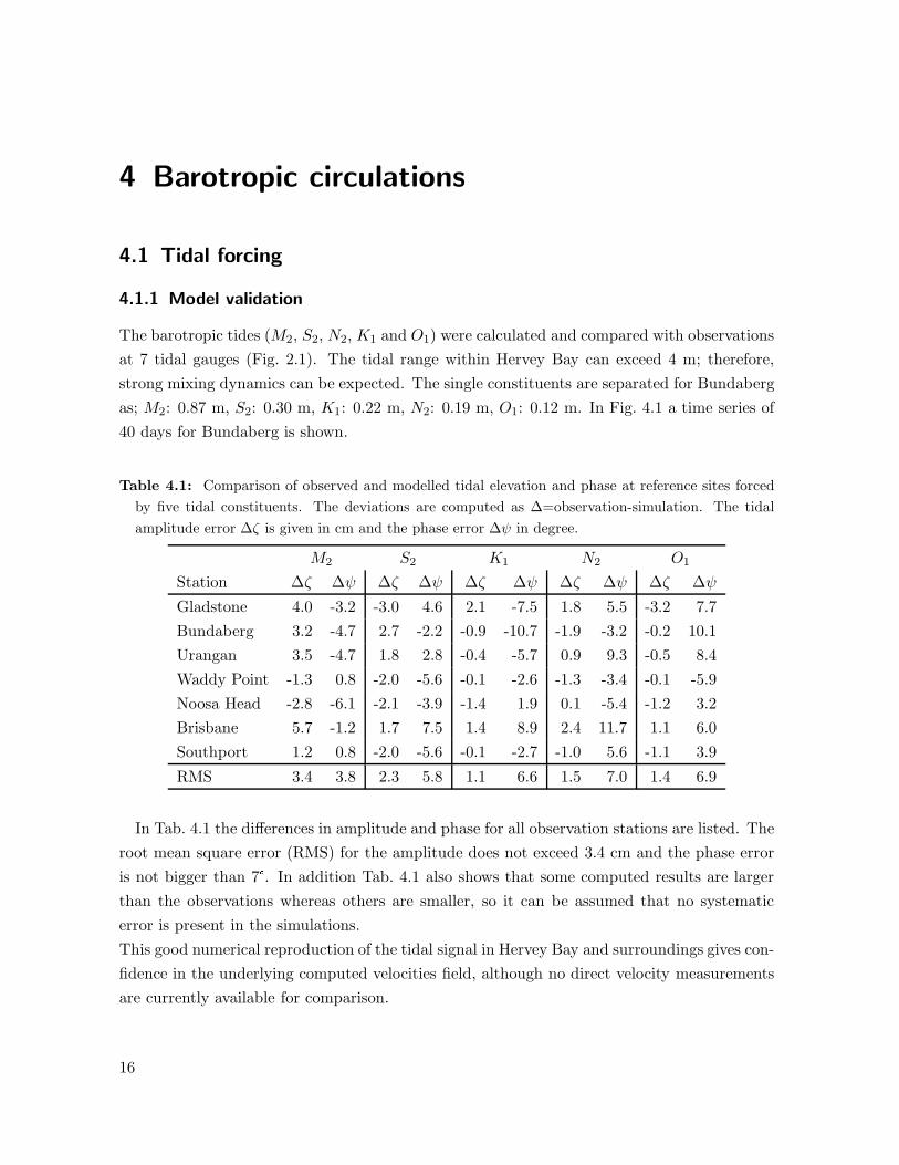
The barotropic tides (M2, S2, N2, K1 and O1) were calculated and compared with observations
at 7 tidal gauges (Fig. 2.1). The tidal range within Hervey Bay can exceed 4 m; therefore,
strong mixing dynamics can be expected. The single constituents are separated for Bundaberg
as; M2: 0.87 m, S2: 0.30 m, K1: 0.22 m, N2: 0.19 m, O1: 0.12 m. In Fig. 4.1 a time series of
40 days for Bundaberg is shown.
Table 4.1: Comparison of observed and modelled tidal elevation and phase at reference sites forced
by five tidal constituents. The deviations are computed as ∆=observation-simulation. The tidal
amplitude error ∆ζ is given in cm and the phase error ∆ψ in degree.
M2 S2 K1 N2 O1
Station ∆ζ ∆ψ ∆ζ ∆ψ ∆ζ ∆ψ ∆ζ ∆ψ ∆ζ ∆ψ
Gladstone 4.0 -3.2 -3.0 4.6 2.1 -7.5 1.8 5.5 -3.2 7.7
Bundaberg 3.2 -4.7 2.7 -2.2 -0.9 -10.7 -1.9 -3.2 -0.2 10.1
Urangan 3.5 -4.7 1.8 2.8 -0.4 -5.7 0.9 9.3 -0.5 8.4
Waddy Point -1.3 0.8 -2.0 -5.6 -0.1 -2.6 -1.3 -3.4 -0.1 -5.9
Noosa Head -2.8 -6.1 -2.1 -3.9 -1.4 1.9 0.1 -5.4 -1.2 3.2
Brisbane 5.7 -1.2 1.7 7.5 1.4 8.9 2.4 11.7 1.1 6.0
Southport 1.2 0.8 -2.0 -5.6 -0.1 -2.7 -1.0 5.6 -1.1 3.9
RMS 3.4 3.8 2.3 5.8 1.1 6.6 1.5 7.0 1.4 6.9
In Tab. 4.1 the differences in amplitude and phase for all observation stations are listed. The
root mean square error (RMS) for the amplitude does not exceed 3.4 cm and the phase error
is not bigger than 7°. In addition Tab. 4.1 also shows that some computed results are larger
than the observations whereas others are smaller, so it can be assumed that no systematic
error is present in the simulations.
This good numerical reproduction of the tidal signal in Hervey Bay and surroundings gives con-
fidence in the underlying computed velocities field, although no direct velocity measurements
are currently available for comparison.
16

4.1 Tidal forcing
4.1.2 Tidal mixing
The hydrodynamical model COHERENS allows to compute the bottom friction velocity and
therefore an estimate of the thickness of the bottom boundary layer or Ekman layer thickness
δ can be given for different flow regimes [Loder and Greenberg, 1986]. The Ekman layer
thickness is a measure to describe a region that is controlled by friction:
δ =c u∗f
(4.1)
where u∗ is the bottom friction velocity, f is the Coriolis parameter and c is a constant that
can vary between 0.1 and 0.4 . The friction velocity u∗ is calculated as√
τB/ρ0, the square root
of the bottom friction normalised by the water density. Therefore, the distribution pattern of
the bottom boundary layer thickness is similar to the bottom friction. Using a low/medium
range value of c = 0.2, the thickness of the tidal (M2) induced Ekman layer in Hervey Bay is
estimated to be of the order of the water depth.
This is a different approach than the usual h/u3 argument, where h is the water depth and u the
depth averaged current speed [Simpson and Hunter, 1974]. However, Simpson and Sharples
[1994] discussed that the Ekman depth should be prefered because it includes directly effects
of rotation on mixing and frontal position. Thus, the Ekman depth measure is chosen.
In Fig. 4.1c the ratio of the Ekman layer thickness divided by the local depth is shown. In the
southern part of Hervey Bay and at Breaksea Spit, the ratio exceeds values of one. Therefore,
the Ekman layer is much thicker than the local depth; hence, friction and turbulent mixing
dominate the whole water column. Thus, one can assume that in these regions, the water
column is well mixed and stratification is suppressed. Only in the central part of the bay and
on the North Western shelf the mixing ratio is smaller than 0.5, hence, only parts of the water
column are occupied by the bottom Ekman layer. Fig. 4.1b shows the maximum M2 induced
tidal currents and the tidal ellipses. It is visible that at Breaksea Spit the currents can reach 1.2
m/s. In the central part of the bay, these currents vary between 0.5 - 0.7 m/s. Here the tidal
ellipses collapse into straight lines and the water is moved only in the north/south direction. It
is assumed that the central part of the bay is also well mixed, because the surrounding regions
supply already well mixed water into the central part by tidal swash transport. Consequently,
tidal mixing, due to the M2-tide alone seems sufficient to completely mix the water column
in Hervey Bay. Hence, only horizontal gradients/fronts are likely to appear. Fig. 4.1a shows
a time series of tidal gauge data at Bundaberg. In the 40 days time series one can see the
fortnightly modulation of the tidal signal. Only during 4-5 days around neap tide the tidal
amplitude is less than the M2 component alone. Therefore, in this short time window, tidal
mixing is significantly reduced and stratification within Hervey Bay can develop.
In Fig. 4.1d the maximum tidal excursion is shown. The pattern is similar to Fig. 4.1a. Peak
values of 8 km are visible at Break Sea Spit and also in the estuary of the Great Sandy Strait.
17

4 Barotropic circulations
0 5 10 15 20 25 30 35 40−2
0
2
time [days]
ampl
itude
[m](a)
(b)
1 m/s
Tidal currents [m/s]
152.4 152.8 153.2
−25.4
−25.2
−25
−24.8
−24.6
−24.4
−24.2
0 0.5 1
(c)
Mixing ratio
152.4 152.8 153.2
0 0.25 0.5 0.75 1 1.25 1.5
(d)
Tidal excursion length [km]
152.4 152.8 153.2
0 2 4 6
Figure 4.1: (a) Typical tidal time series for Bundaberg. Indicated by the red dashed line is theamplitude of the M2 component, (b) maximum tidal currents (M2) and plot of the tidal ellipse and(c) the ratio Ekman layer/local depth and (d) the tidal excursion. For visualisation purposes, themixing ratio is limited to 1.5. The averaging period is five tidal cycles.
In most parts of the bay and on the northern shelf, the horizontal displacement during a tidal
cycle is less than 2 km.
4.2 Residual circulations
Fig. 4.2 shows that the M2 induced residual transport is negligible. In most parts of the bay,
the residual currents are less than 1 cm/s. Only at Breaksea Spit and in the northern part of
the Great Sandy Strait they can reach values of 10-15 cm/s. The contributions of the other
four tidal constituents to the residual flow are negligible. The importance of rotation of the
flow is also negligible. In most parts of the bay, it is far less than 0.1 cycles/day. Only at
Breaksea Spit and in the mouth region of the Great Sandy Strait peak values exists of approx.
1 cycles/day. Therefore, the tide in Hervey Bay is mainly responsible for the vertical mixing,
but transport processes are dominated by wind and baroclinic forcing. This feature of Hervey
Bay is quite surprising. Due to the high tidal range, much stronger residual currents should be
expected. Furthermore, numerical experiments (not shown here) with barotropic conditions
and variations in bottom roughness did not change the residual circulation significantly. It
must be concluded that weak residual currents are an intrinsic feature of Hervey Bay.
The region of Hervey Bay is influenced by the Trade winds from the east with a northern
component (NE wind) in autumn and winter and a southern one in spring and summer (SE
wind) (Tab. 2.1) with an average strength of 6-7 m/s. Because both wind directions are
18

4.2 Residual circulations
dominant and represent different residual circulations, only these two directions are considered.
(a)
152.4 152.8 153.2−25.4
−25.2
−25
−24.8
−24.6
−24.4
−24.2
(b)
152.4 152.8 153.2−25.4
−25.2
−25
−24.8
−24.6
−24.4
−24.2
(c)
152.4 152.8 153.2−25.4
−25.2
−25
−24.8
−24.6
−24.4
−24.2
5 10 15
Figure 4.2: Depth averaged residual circulations and currents (in cm/s) for (a) M2, (b) idealised NE
wind (6 m/s) and (c) idealised SE wind (6 m/s). The magnitude is indicated by the colour code,
whereas the arrows are normalised to indicate the direction of the flow. Residual currents below 1
cm/s are marked white. The averaging period is one spring-neap cycle. The residual currents for the
wind forcing are detided by subtracting the tide induced residuals.
During SE winds a clockwise current exists in the bay (see Fig. 4.2c). Ocean water enters
the bay via Breaksea spit and leaves Hervey Bay along the western shore. Peak values of 15
cm/s are reached in the shallow waters in the western part of the bay. The average residual
transport is computed with 4 cm /s. Further east of Break Sea Spit the wind-induced currents
reaches peak values of 18-20 cm/s. Thus, during SE wind there exist a narrow near shore
current, which is trapped between Fraser Island and the 150 m depth contour. Break Sea Spit
shields Hervey Bay from this current. Water passing the spit enters the bay to leave past a
U-Turn at the western shore. Nevertheless, most of the water of this coastal current flows
19

4 Barotropic circulations
northward, to turn at the northern end of Break Sea Spit to the west/north-west, to flow into
the direction of the Great Barrier Reef, without any water exchange with Hervey Bay.
For NE-wind conditions, the whole circulation pattern changes. Now the bay is dominated by
an anti-clockwise circulation. Further, the residual circulation velocity is reduced. Maximum
flow velocities are 8 cm/s and the averaged flow speed is 2-3 cm/s. Only at the eastern shore,
a 5 km narrow jet exists, where the flow speed reaches 15-18 cm/s. The coastal current at the
eastern side of Fraser Island also reverses its direction. At the northern end of Hervey Bay
a clockwise circulations cell exists, which is trapped between Break Sea Spit and Lady Elliot
Island in the north. Therefore, water is exchanged with the northern shelf. Interesting to note
is the stream that flows between Lady Elliot Island and the northern tip of Break Sea Spit. It
transports water as a bottom flow within the Mary River Canyon. This feature will be later
important for the baroclinic water exchange with the open ocean. At the northwestern part
of the shelf exists a secondary circulation cell that restricts the water exchange between the
northern shelf and the Bay.
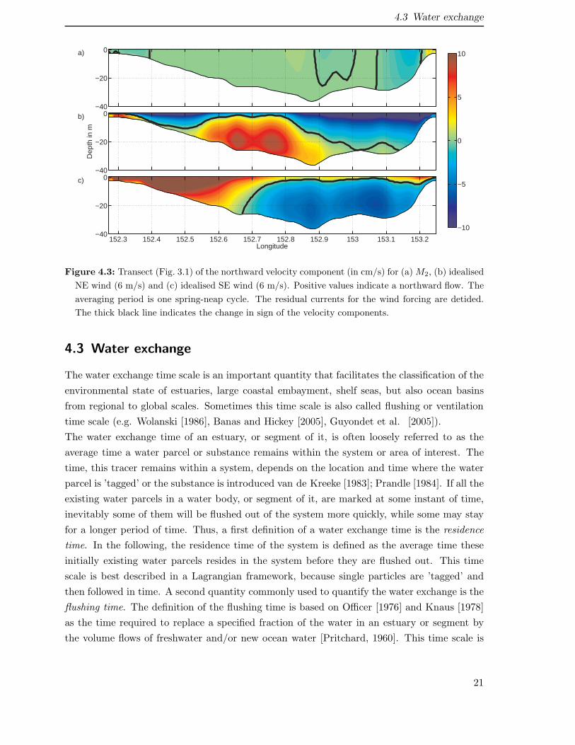
To give a better understanding of the three dimensional circulation, in Fig. 4.3 a transect of
the residual meridional velocity component at the northern end of Hervey Bay is shown. Fig.
4.3b depicts that during NE wind a two-layered structure exists. Surface water flows into the
bay and leaves in a central jet at the seafloor. Surface current speeds can reach 15 cm/s,
whereas the flow speed in the central outflow jet is approx. 10 cm/s. For SE wind (Fig. 4.3b)
the bay shows a east/west separation. Water enters the bay at the eastern part and leaves
Hervey Bay at the shallow western shore. However, there exists also a thin northward-directed
surface flow in the eastern part. For completeness, also the residual current for the tide is
given in Fig. 4.3a. As expected, the currents are negligible small.
Combining Fig. 4.1b and Fig. 4.2b,c can indicate possible scenarios for stratification in Hervey
Bay. During SE wind, well mixed water at Break Sea Spit is flushed into the bay. This can
prevent the occurrence of stratification. During NE wind water from the northern shelf enters
the bay. Due to low mixing in this region, the water column can be stratified and therefore
this layered water is pushed into the bay and can therefore establish stratification in Hervey
Bay. Further, the bottom outflow of dense water, generated within the bay, can slide under
lighter water on the shelf. The residual circulation cell (Fig. 4.2b) and the two layered flow
structure (Fig. 4.3b) can lead to a positive feedback loop, which enhances the stratification
in the bay and at the shelf. Nevertheless, one has to keep in mind that NE wind is mostly
dominant during the southern hemisphere winter, where stratification is generally unlikely.
However, this feature will be later important for the release and triggering of gravity currents
(see chapter 7).
20
4.3 Water exchange
Dep
th in
m
b)
−40
−20
0
−10
−5
0
5
10a)
−40
−20
0
Longitude
c)
152.3 152.4 152.5 152.6 152.7 152.8 152.9 153 153.1 153.2−40
−20
0
Figure 4.3: Transect (Fig. 3.1) of the northward velocity component (in cm/s) for (a) M2, (b) idealised
NE wind (6 m/s) and (c) idealised SE wind (6 m/s). Positive values indicate a northward flow. The
averaging period is one spring-neap cycle. The residual currents for the wind forcing are detided.
The thick black line indicates the change in sign of the velocity components.
4.3 Water exchange
The water exchange time scale is an important quantity that facilitates the classification of the
environmental state of estuaries, large coastal embayment, shelf seas, but also ocean basins
from regional to global scales. Sometimes this time scale is also called flushing or ventilation
time scale (e.g. Wolanski [1986], Banas and Hickey [2005], Guyondet et al. [2005]).
The water exchange time of an estuary, or segment of it, is often loosely referred to as the
average time a water parcel or substance remains within the system or area of interest. The
time, this tracer remains within a system, depends on the location and time where the water
parcel is ’tagged’ or the substance is introduced van de Kreeke [1983]; Prandle [1984]. If all the
existing water parcels in a water body, or segment of it, are marked at some instant of time,
inevitably some of them will be flushed out of the system more quickly, while some may stay
for a longer period of time. Thus, a first definition of a water exchange time is the residence
time. In the following, the residence time of the system is defined as the average time these
initially existing water parcels resides in the system before they are flushed out. This time
scale is best described in a Lagrangian framework, because single particles are ’tagged’ and
then followed in time. A second quantity commonly used to quantify the water exchange is the
flushing time. The definition of the flushing time is based on Officer [1976] and Knaus [1978]
as the time required to replace a specified fraction of the water in an estuary or segment by
the volume flows of freshwater and/or new ocean water [Pritchard, 1960]. This time scale is
21

4 Barotropic circulations
well suited for the Eulerian framework, because it is necessary to compute the concentration
at a specific point or region. Both definitions of water exchange are based on the displacement
concept, which gives the time required to displace all the water in the region under consider-
ation.
Using domain averaged time scales, they are single parameters representing the integral time
scale of all physical transport processes of the system at once, which may be used to be com-
pared to time scales of biological and chemical processes or baroclinic response. Zimmerman
[1988] also defined several local time scales, which are functions of location in estuaries. The
local time scales provide more detailed information, however they suffer from complication
when related to biogeochemical processes.
It is obvious that the residence time of an estuary will change with its flushing time. The longer
it takes to flush an estuary, the longer its residence time will be. The flushing of estuarine
waters is achieved by all the mechanisms effecting the transport or removal of water from the
estuary to the open sea. These transport mechanisms include tidal flushing, river discharge,
density induced estuarine circulation and those induced by meteorological events.
4.3.1 Setup
In the following three different scenarios are used which are identical to the setups of the
computation of the residual circulations. Therefore, the model is forced with the tide without
wind, tide and NE wind (6 m/s) and finally tide and SE wind (6 m/s). The duration of the
experiments is limited to 60 days of constant forcing. Although it seems unrealistic to consider
a constant NE wind for 2 months, these idealised experiments shall give a rough estimate of
the water exchange. At the southern boundary the flow rates, through the Great Sandy Strait,
from Tab. 4.2 are imposed. These values are taken from the outer model.
Table 4.2: Tidal averaged flow through the Great Sandy Strait in m3/s. Negative values indicate
southward transport.
Tide NE wind SE wind
transport -100 -1200 800
van de Kreeke [1983] further differentiated the phase of the tide when the particles/tracer
were initially released. Due to the weak tidal residual currents and the fact that the spatial
dimension of the bay is much larger than the tidal excursion (Fig. 4.1c), the dependence on the
tidal phase is insignificant. Further, the dependence of the water exchange on the spring-neap
cycle was neglected. Additional experiments (not shown here) where the release was at spring
tide and one experiment with a release at neap tide, showed that the differences are negligible.
22

4.3 Water exchange
Flushing time
To compute the flushing time, the bay is filled with a neutral buoyant passive tracer, where
in every grid cell within the bay the concentration is set to one. The northern boundary of
the bay is given in Fig. 3.1. Then for every grid cell, the time is computed until the local
concentration drops below a threshold. Thus
Tflushing = T (C(t) > Cthreshold) (4.2)
The threshold Cthreshold is set to 1/e, where e is the Euler number. Therefore, the flushing
time is equivalent to the e-folding time.
Residence time
To asses the residence time, neutrally buoyant particles (which shall represent water parcels)
are released within the bay. Particles were tracked entirely in post processing; using Fortran
code that integrates the 3D velocity fields from COHERENS saved every 15 min. A multistep
scheme (HEUN scheme) was used for the integration, with a time step of 60 s in the horizontal
and 3 s in the vertical. In addition to advection in all three dimensions, particles were subject
to horizontal/vertical diffusion, using the ’random displacement’ scheme described by Visser
(1997). This scheme adds a random velocity, scaled by the local diffusivity from COHERENS,
to the advective velocity at every time step, and further includes a correction based on the
local diffusivity gradient:
dX(t) = (u+ ∂x KH)dt +√
2KH dWx(t)
dY (t) = (v + ∂x KH)dt+√
2KH dWy(t)
dZ(t) = (w + ∂x KV )dt+√
2KV dWz(t)
(4.3)
where X,Y,Z is the position, dt the time step, u, v,w the advective velocity, dWx, dWy, dWz
independent noise increments with mean 0 and variance dt, and KH the horizontal diffusivity
and KV the vertical one. The gradient correction is essential to preventing particles from
accumulating unrealistically in low-diffusivity areas, as demonstrated by [Visser, 1997]. For
a detailed discussion on the underlying theory and the validation of the numerical particle-
tracking scheme, the reader is referred to appendix A.
23

4 Barotropic circulations
(a)
152.4 152.8 153.2
−25.4
−25.2
−25
−24.8
10 20 30 40 50
(b)
152.4 152.8 153.2
−25.4
−25.2
−25
−24.8
(c)
152.4 152.8 153.2
−25.4
−25.2
−25
−24.8
0 20 400
0.5
1(d)
Tide
NE wind
SE wind
Figure 4.4: Depth averaged flushing time. The colour code indicates the time in days, for (a) tide, (b)
tide + NE wind, (c) tide + SE wind and (d) normalised bay averaged concentration. The critical
threshold Cthreshold is indicated by the black dashed line.
4.3.2 Flushing time
In Fig. 4.4a-c the local e-folding renewal time is shown. Clearly visible in Fig. 4.4a is that
the tide does not contribute to the water exchange. This was expected due to the very small
residual currents. During the two month of simulations, only the most north-eastern part
could be flushed.
The water exchange changes dramatically if additional wind forcing is imposed. During NE
wind (Fig. 4.4b) most of the bay water is flushed within 20 days. Especially the eastern part
of the bay shows flushing times of less than 10 days. Clearly visible is the impact of the costal
jet, at the eastern shore, on the water exchange. In the central northern part of the bay, the
flushing time yields values of more than 50 days. This is caused by the fact, that most of
the water leaves Hervey Bay through the bottom jet (Fig. 4.3b). Therefore, the concentration
remains high until all bay water has left. At the western shore, there also exists a narrow
24

4.3 Water exchange
region, which shows rapid response to NE wind forcing. The flushing time of the Great Sandy
Strait is approx 25 days. During NE wind, a southward flow exists in the strait system. Thus
bay water is flowing through the strait and keeps the concentration high.
During SE wind the water exchange in the Strait is much faster (Fig. 4.3c). Now a northward
flow pushes ’new’ water into the bay and leads therefore to a fast water exchange in the mouth
of the Great Sandy Strait. The U-styled residual circulation within the bay is also visible in
the flushing time pattern. Fresh water is entering the bay in the eastern part and leaving the
bay at a narrow coastal stripe at the western shore. A stationary eddy causes the high flushing
times in the eastern part. This circulation cell close to Fraser Island is also visible in Fig. 4.2c.
The water exchange in the southern part of the bay is much slower than for NE wind.
In Fig. 4.4d the bay averaged concentration for the three forcing scenarios is given. The critical
thresholf of 1/e was crossed for SE wind at around 20 days, for NE wind 43 days, respectively.
For only tidal forcing, the threshold was not reached during the two months of simulation.
For the case of NE wind, the impact of the large circulation cell at the northern shelf is cleary
vissible(Fig. 4.2b). The bay shows a rapid response to this forcing. After approx. 14 days,
waters that were flushed out of the bay due to this cell, enter the bay again and therefore keep
the concentration high.
To quantify the rapid response, it is assumed that for short timescales, the concentration in
the bay drops exponentially. Thus to the first 10 days of the concentration time series, an
exponential fit was applied of the form:
C(t) = exp
(
− t
τ
)
(4.4)
τ gives then the decay rate. The results are summarised in Tab. 4.3. With a decay rate of 12
days for NE wind, the response time is much faster than for SE wind with 25 days. The decay
rate for the tidal forcing is approx. 3 months.
Table 4.3: Water exchange times for three different forcing scenarios. Given are the flushing times in
days for the threshold method and the exponential decay rate.
Tide NE wind SE wind
Threshold - 43 20
Exp. decay 130 12 25
Fig. 4.4d shows, that there exist two different times scales for Hervey Bay. A fast mode,
covering exchange processes within 3 weeks and secondly a slow mode, for the response when
the fast mode decayed. The fast mode is only visible for the wind forcing, thus indicating ex-
change processes associated with wind-induced circulations. Within 3 weeks, the concentration
drops rapidly and can be described by an exponential decay, with a decay rate of approx. 20
days. After the three weeks, Hervey Bay enters into the slow mode. The drop in concentration
25

4 Barotropic circulations
is much lower and comparable for the three forcing scenarios. The decay rate is reduced to
approx. 3 months.
4.3.3 Residence time
The residence time is defined as the time required for a particle to travel from a location,
within the system, to the boundary of the region [Prandle, 1984], therefore it is dependent of
the location where the particle is released. Sometimes the residence time is also called turn
over time. To compute this time scale, 107 uniformly distributed particles are released in the
bay. Then, every particle is followed over 2 months and the time is computed until the particle
crosses the northern/southern boundary of the bay.
(a)
152.4 152.8 153.2
−25.4
−25.2
−25
−24.8
−24.6
10 20 30 40 50 60
(b)
152.4 152.8 153.2
−25.4
−25.2
−25
−24.8
−24.6
(c)
152.4 152.8 153.2
−25.4
−25.2
−25
−24.8
−24.6
Figure 4.5: Depth averaged residence time. The color code indicates the time in days, for (a) tide,
(b) tide + NE wind and (c) tide + SE wind.
Because at every grid point, approx. 4000 particles are initialised in the whole water column,
the depth averaged residence time for these 4000 particles is calculated. The results are shown
in Fig. 4.5. Due to the weak tidal residual currents, also the tidal residence time is high. Only
at the northern end of the bay, particles leave the bay due to tidal excursion and diffusion.
In the mouth of the Great Sandy Strait, residence times are also low due to the southward
26

4.3 Water exchange
directed residual flow through the strait (Tab. 4.2). The central part of the bay is not affected
by the tide. This changes dramatically by imposing NE wind. Residence times in the western
part are approx. 5-15 days. In the eastern part, particles need 30-50 days to leave the bay.
Thus, the pattern of the residence time clearly reflects the residual circulation. Because water
enters the bay at the eastern part, it has to be carried the whole way trough the bay, to exit
at the central part.
For SE wind the pattern is similar. The residence times of the western part of the bay is less
than 10 days. Due to the strong northward-directed flow in the Great Sandy Strait, Hervey
Bay shows a clear east/west separation. Waters originating from the Great Sandy Strait are
effectively transported along the western shore. At the eastern shore, the trapping of particles,
due to a persisted circulation cell, is visible. Here, residence times can reach 50-60 days.
4.3.4 Origin of replacement water
The particle-tracking scheme further allows to asses the origin of the replacement water, thus
answering the question: Where do the waters, entering Hervey Bay, come from? This is
computed by inverting the setup of the residence time. Again 107 particles are released, but
now they are initialised outside the bay. Than the time is computed until the particles cross
the boundaries of Hervey Bay and thus entering the bay domain. In Fig. 4.6 only the results
for wind forcing are shown.
(a)
152.4 152.8 153.2−25.5
−25
−24.5
0 10 20 30 40 50
(b)
152.4 152.8 153.2−25.5
−25
−24.5
Figure 4.6: Depth averaged replacement time. The colour code indicates the time in days, for (a) tide
+ NE wind and (b) tide + SE wind.
For NE wind (Fig. 4.6a), only water from the northern shelf enters the bay. Due to the large
residual circulation cell, bounded by Break Sea Spit and Lady Elliot Island (see Fig. 4.2b), the
water is trapped and the water exchange with the open ocean is limited.
27

4 Barotropic circulations
For SE wind conditions (Fig. 4.6b) open ocean water enters the bay via Break Sea Spit. The
simulations show that within 10 days, shelf water (east of Fraser Island) replaces water in
Hervey Bay.
28

5 Baroclinic processes
5.1 Model Validation
Because the simulations reveal that the bay is in parts vertically well mixed throughout most
of the year, the depth averaged salinity/temperature distribution is considered here for the
first model validation. The simulated temperature and salinity distribution within Hervey
Bay is consistent with the observations during all three field surveys (Fig. 5.1). The model
reproduces the salinity gradient with salinity decreasing in all three field trips from the south
west coast towards the northern opening of the Bay (Fig. 5.1).
observation
(a)
simulation
(b)
(c)
Salinity [psu]152.4 153
152.4 153
35 35.5 36 36.5
observation
−25.2
−24.6simulation
−25.2
−24.6
Temperature [°C]152.4 153
−25.2
−24.6
152.4 153
20 22 24 26
Figure 5.1: Comparison of the depth-averaged salinity and temperature distributions during (a)
September 2004, (b) August 2007 and (c) December 2007.
The comparison with the first survey shows that the salinity gradient is less sharp than
indicated by the model. In general, the agreement of the model output and the measurements
from each of the field trips is quite well. The model confirms that the coastal region is
occupied by a zone of hypersalinity with salinities well above 36 psu. The model reproduces
the observed temperature distribution as well. There are some deviations for the September
2004 field trip. The model seems to overestimate the temperature in the near shore region, but
29

5 Baroclinic processes
both observations and simulated data show a similar pattern. The distribution of temperature
is matched by the model for both subsequent field trips.
For further validation, transects of temperature and salinity at the northern opening of Hervey
Bay are shown in Fig. 5.2. The coastal hypersalinity zone is somewhat wider than the model
indicates, but again the patterns are matched. The model also reproduces the bottom cold-
water pool for the first two field trips.
observation
(a)
−20
−10
0simulation
Dep
th in
m
(b)
−20
−10
0
(c)
Salinity [psu]152.6 152.9
−20
−10
0
152.6 152.9
35 35.5 36 36.5
observation
−20
−10
0simulation
−20
−10
0
Temperature [°C]152.6 152.9
−20
−10
0
152.6 152.9
20 22 24 26
Figure 5.2: Comparison of the salinity and temperature transects along 24.8°S latitude (a) September
2004, (b) August 2007 and (c) December 2007.
The temperature pattern for the September 2004 field trip, reflects the residual circulation
pattern for NE wind (Fig. 4.2b), which was observed during this field campaign. Cold water
leaves the bay in the central part and creates therefore the central cold-water pool. Further,
the two layered structure (Fig. 5.2a) agrees with the barotropic residual flows (Fig. 4.3b).
To show that the model also captures the dynamics on the shelf, transects of σt density in
the northern part of Hervey Bay are shown in Fig. 5.3. The model misses the proper timing
of the upwelling event, which is visible in the observation for December 2007. It seems that
this event is lagged by two days in the simulations. For the May and June 2008 field trips,
the agreement is quite well. The model reproduces the frontal structures and the vertical
well-mixed conditions on the shelf.
30

5.1 Model Validation
observation
(a)
−40
−20
0simulation
Dep
th in
m
(b)
−40
−20
0
(c)
152.2 152.6 153.0
−40
−20
0
Longitude
152.2 152.6 153.0
23 23.2 23.4 23.6 23.8 24 24.2 24.4 24.6 24.8 25
Figure 5.3: Comparison of σt density [kg/m3] transects; (a) along 24.5°S during December 2007, (b)along 24.4°S during May 2008 and (c) along 24.5°S during June 2008.
2 4 6 8 10
2
4
6
8
10
Esimu
Epa
n
y = 0.940*x + 0.384
R2 = 0.794
(b)
20 25 30
20
25
30
SSTsimu
SS
TA
VH
RR
y = 0.980*x + 0.451
R2 = 0.818
(a)
Figure 5.4: Scatter plot of a) simulated SST vs. AVHRR SST [K] and b) simulated evaporation vs.
measured pan evaporation [mm/day]. The red line indicates a linear fit.
In order to demonstrate the model performance to capture the dynamics on longer time
scales, satellite AVHRR SST data for the period 1999 - 2005 have been used for the model
validation. Fig. 5.4a shows the comparison of bay averaged model SST data and AVHRR
satellite data. The linear fit indicates that the model reproduces the measurements with a
vanishing bias. R2 with 0.82 is quite high.
The comparison between the measured and simulated evaporation is shown in Fig. 5.4b (for
31

5 Baroclinic processes
Bundaberg (1997-2008)). Due to the expected higher sampling errors in the pan-evaporation
measurement the data scatter is wider. Again R2 with 0.8 is reasonably high. The linear fit
again indicates that the model tends to underestimate high evaporation rates and vice versa
overestimates low evaporation rates, but this systematic error is quite small.
The simulated southward transport of the East Australian Current is on average 7.1 Sv, which
is much less than the EACs seasonal average of 16.2 Sv (see Tab. 2.1). Further, the location of
the centre of the EAC is shifted in the simulations in the northern part of the model domain
towards the 1000 m depth contour by 30-40 km. However, given the unrealistic maximum
depth of 1100 m, this transport is assumed to be representative of a baroclinic EAC flow.
[Oke and Middleton, 1999] also used the same argument.
32

5.2 Stratification within Hervey Bay
5.2 Stratification within Hervey Bay
The stratification is expressed in terms of a scalar quantity φ [Simpson et al. , 1990], which is
defined as:
φ =1
H
∫ 0
−H(ρ− ρ(z))gz dz; with ρ =
1
H
∫ 0
−Hρ(z) dz (5.1)
where ρ(z) is the density profile of the water column of depth H. φ (units J/m−3) is the work
required to bring about complete mixing. Recently, this quantity has been also defined as a
potential energy anomaly (PEA) (see e.g. Røed and Albertsen [2007]).
1990 1992 1994 1996 1998 2000 2002 2004 2006−0.6
−0.4
−0.2
0d)
time [year]
∆ S
−0.4
−0.2
0
c)
∆ ρ
0
5
10
15b)
φ
0.10.20.30.40.5a)
τ
Figure 5.5: (a) Time series of wind stress - τ [Pa], (b) stratification index - φ [Jm−3], (c) difference
between surface and bottom density - ∆ρ [kgm−3] and (d) difference between surface and bottom
salinity - ∆S [psu]. Time series for (b), (c) and (d) are only computed in the bay where the depth
is greater than 15 m. Shown are daily averaged values.
φ is therefore an expression for the competition of stirring (wind stress, tides, waves and cur-
rents) and stratification (heating and buoyancy flux due to precipitation and river discharge).
Fig. 5.5 gives time series of daily averaged wind stress, surface to bottom density/salinity
difference and φ. The time series of ∆ρ yield that the maximum difference is of the order
0.4 kgm−3. These peak values appear mostly in spring and early summer. Cold “winter”
water resides at the bottom of Hervey Bay, whereas increasing solar heat flux increases the
temperature of the upper layers and hence establishes the density difference. It is interesting
to note that the time series is rather spiky. The time lag between the spikes is nearly an in-
teger multiple of 14 days and clearly shows the spring/neap cycle of the tide. Fig. 5.6 depicts
the spectral analysis of the bay averaged stratification index. The pronounced peaks at 14
and 28 days cleary show the influence of the spring/neap cycle on φ and thus the fortnightly
33

5 Baroclinic processes
tidal modulations. Therefore during spring tide, tidal mixing almost completely removes any
stratification and only during neap tide a short-term stratification (< 6 days) can be seen.
Further the daily, annual cycles and the M2-cycle are visible,.
0.5 1 14 28 365 7300
0.05
0.1
0.15
0.2
Periode in days
PS
D
M2
daily
annual
Figure 5.6: Power spectral density (PSD) of the bay averaged stratification index φ (1990-2008). The
sampling frequency is 2 hours.
The following analysis is mainly focused on daily averages, excluding daily cycles and inter-
tidal effects (tidal straining). During winter, there is no stratification visible. The same signal
can also be seen in the time series of φ. Most of the time it is less than 2 Jm−3 and only in
spring and summer the required energy to bring about complete mixing can exceed 5 Jm−3.
In contrast, the time series of ∆S is nearly flat. Almost during the whole year, the surface to
bottom salinity difference vanishes and only during some rare events, the difference can reach
-0.4 psu. Negative differences are caused by rainfall events. Positive peaks are associated with
bottom flows of cold, “fresh” dense water because these peaks mostly occur during late au-
tumn. This rather flat time series indicates that the main contribution to stratification is from
thermal effects. A second reason for dominating thermal stratification is the short duration of
these events. There is not enough time that saline two layer structures can develop.
An additional source of mixing is energy input due to wind stress (Fig. 5.5a). Under light
wind conditions thermal stratification can develop (as expected) but the additional wind en-
ergy input during medium/high wind conditions, can completely mix the water column even
during neap tide.
34

5.3 Inverse state and hypersalinity
5.3 Inverse state and hypersalinity
The hydrographic observations made during the three field surveys indicate that hypersalin-
ity is likely to be a reoccurring climatological feature characterising the bay. Climatological
data for evaporation, precipitation and river runoff (see Tab. 2.1) show that evaporation with
about 2 m/year by far exceeds the supply of freshwater into the bay from precipitation with
about 1 m/year and very low river run-off (see Ribbe [2006] for details). The application of
the ocean model allows investigating the distribution of salinity throughout time. In fact, the
time-averaged distribution of salinity in the bay (Fig. 5.7) and its surroundings confirms that
the hypersalinity zone is a climatological feature for the period 1990-2008. The climatological
mean value for the salinity gradient in the bay is in the order of about 0.5 psu with salinities
near the south west of > 36.1 psu and near the open ocean in the north east of about < 35.5
psu. The magnitude of these gradients correspond to those observed during the three surveys.
To describe the temporal evolution of the hypersalinity zone within Hervey Bay, the salin-
Longitude
Latit
ude
36
35.9
35.8
35.7
35.6
35.5
35.6
152 152.5 153 153.5
−26
−25.5
−25
−24.5
−24
Figure 5.7: Mean salinity distribution averaged over the period 1990-2008. Also shown is the positionof the three transects to compute the density and salinity gradients.
ity/density gradients along the indicated transects in Fig. 5.7 have been computed. Firstly,
the focus is on the transect that is placed at the northern end of Hervey Bay. The transect is
35

5 Baroclinic processes
aligned perpendicular to the isolines of the climatological salinity distribution. Fig. 5.8 pro-
vides an indication of the temporal evolution of these gradients. They are plotted as psu/km
and kg/m3/km.
To quantify these gradients the approach of Largier et al. [1997] is followed in defining hy-
persalinity and the inverse state of an estuary/bay as: “... hypersaline is defined as salinities
significantly greater than that of the ambient and inverse as densities significantly greater than
that of the ambient... ”. By salinities significantly greater, the authors define a salinity S that
exceeds the ambient salinity S0 by more than typical synoptic (i.e. multi-day) fluctuations in
the salinity of the ambient coastal waters. The standard deviation of the ambient salinity over
the period of hypersalinity, serves as an appropriate index of the size of these fluctuations.
Thus, (S − S0) > σ defines hypersalinity. For the case of Hervey Bay these fluctuations are of
the order σ=0.15 psu and in terms of the salinity gradient σGrad ≈ 2 · 10−3 psu/km and there-
fore one third of the climatological gradient. This means that Hervey Bay can be classified as
a hypersaline bay.
To define the inverse state a dynamical approach is used here. To have a Hervey Bay specific
threshold for the inverse state, the density gradients are converted into geostrophic induced
velocities, serving as a rough indication. Because tidal mixing is quite high and therefore tur-
bulence is essential in this coastal environment as demonstrated above, this indicator should
be handled with care.
Computing the geostrophic residual velocity, caused by a mean density difference of 0.45 kg/m3
over a distance of 65 km (see Fig. 5.7), will result in a flow of approx. 3-5 cm/s. This is in
the range of the wind induced residual circulations (Fig. 4.2). Here a wind speed of 6 m/s is
assumed, which is the mean climatological average. Hence, a geostrophic flow could balance a
northerly wind induced circulation. Thus density gradients exceeding 0.01 kgm−3/km can be
dynamically important for Hervey Bay.
In Fig. 5.8ab the red dashed lines indicate these critical values. As stated in the description
of Hervey Bay, a special feature of it is an aspect ratio of nearly one, i.e. the width of the
connection to the open ocean is equal to the length of the bay itself. For Spencer Gulf, Gulf
of California and Ria of Pontevedra this ratio exceeds a value of three. Therefore Hervey
Bay is better described as an “open” coastal environment than to fit into a classical inverse
estuary type classification. Further due to its low aspect ratio the bay can not produce high
salinity/density gradients like for instance Spencer Gulf with peak salinities of > 50 psu in the
headwater of the gulf.
36

5.3 Inverse state and hypersalinity
b)
∂ S
−0.02
0
0.02
a)
∂ ρ
−0.02
0
0.02
Year
Day
s
c)
1990 1995 2000 2005
50
150
250
350
Figure 5.8: a) Time series of density gradient - ∂ρ [kg/m3/km], b) salinity gradient - ∂S [psu/km].
Shown are daily averages. The red dashed lines indicate the thresholds given in the text and c)
depicts the number of days per year where hypersaline (stars)/inverse (circles) conditions are found.
To indicate the trend, linear fits are added. The grey bars show El Nino/La Nina events.
To understand if these gradients are Hervey Bay specific or if they reflect simply the varia-
tion in the usual subtropical near shore hypersalinity zone [Tomczak and Godfrey, 2003], two
additional transects (see Fig. 5.7) have been investigated in the model domain. One is situated
at the northern shelf of Hervey Bay and the other is placed approx. 80 km south of Fraser
Island.
Tab. 5.1 shows the comparison of the two additional transects with the gradients in Hervey
Bay. The density and salinity gradients are a factor of two higher than the ones computed at
the northern shelf. Interesting to note is, that the mean values for the southern transect are
nearly vanishing. Comparison of the standard deviation of the three transects demonstrates
37
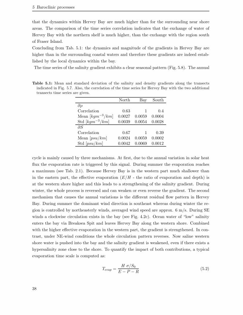
5 Baroclinic processes
that the dynamics within Hervey Bay are much higher than for the surrounding near shore
areas. The comparison of the time series correlation indicates that the exchange of water of
Hervey Bay with the northern shelf is much higher, than the exchange with the region south
of Fraser Island.
Concluding from Tab. 5.1: the dynamics and magnitude of the gradients in Hervey Bay are
higher than in the surrounding coastal waters and therefore these gradients are indeed estab-
lished by the local dynamics within the bay.
The time series of the salinity gradient exhibits a clear seasonal pattern (Fig. 5.8). The annual
Table 5.1: Mean and standard deviation of the salinity and density gradients along the transectsindicated in Fig. 5.7. Also, the correlation of the time series for Hervey Bay with the two additionaltransects time series are given.
North Bay South
∂ρCorrelation 0.63 1 0.4Mean [kgm−3/km] 0.0027 0.0059 0.0004Std [kgm−3/km] 0.0039 0.0054 0.0028
∂SCorrelation 0.67 1 0.39Mean [psu/km] 0.0024 0.0059 0.0002Std [psu/km] 0.0042 0.0069 0.0012
cycle is mainly caused by three mechanisms. At first, due to the annual variation in solar heat
flux the evaporation rate is triggered by this signal. During summer the evaporation reaches
a maximum (see Tab. 2.1). Because Hervey Bay is in the western part much shallower than
in the eastern part, the effective evaporation (E/H - the ratio of evaporation and depth) is
at the western shore higher and this leads to a strengthening of the salinity gradient. During
winter, the whole process is reversed and can weaken or even reverse the gradient. The second
mechanism that causes the annual variations is the different residual flow pattern in Hervey
Bay. During summer the dominant wind direction is southeast whereas during winter the re-
gion is controlled by northeasterly winds, averaged wind speed are approx. 6 m/s. During SE
winds a clockwise circulation exists in the bay (see Fig. 4.2c). Ocean water of “low” salinity
enters the bay via Breaksea Spit and leaves Hervey Bay along the western shore. Combined
with the higher effective evaporation in the western part, the gradient is strengthened. In con-
trast, under NE-wind conditions the whole circulation pattern reverses. Now saline western
shore water is pushed into the bay and the salinity gradient is weakened, even if there exists a
hypersalinity zone close to the shore. To quantify the impact of both contributions, a typical
evaporation time scale is computed as:
Tevap =H σ/S0
E − P −R(5.2)
38

5.4 Evaporation induced circulations
where H denotes the mean depth, σ the size of the salinity fluctuations around S0 and in the
denominator are the contributions of the fresh water balance (evaporation, precipitation and
river discharge).
This gives an average Tevap of 15 days. In Tab. 4.3 typical water exchange time scales for
Hervey Bay are given as 20-40 days. Therefore, the evaporation water loss dominates the
salinity gradient rather than the movement of saline water due to residual circulations.
A third, more random, mechanism is provided by significant rainfall events accompanied by
somewhat delayed higher river discharges, i.e. the salinity near the coast is lower than towards
the open ocean. This is for example the case during 1996 when the strongest reversal is
observed. Closer inspection of the time series (not shown here) for surface freshwater fluxes due
to rainfall and river discharges reveal that during this year a particular wet winter prevents the
maintenance of a hypersalinity zone from about April to November 1996. With the approach
of summer and an increase of evaporation and no further significant freshwater discharges, the
hypersalinity zone reforms (Fig. 5.8b).
5.4 Evaporation induced circulations
Due to the net loss of water (by evaporation) and to maintain the waterbalance within the
bay, an inflow of water from the ocean is required. Tab. 2.1 shows that the annual loss of
water is approx. 800 mm or 130 m3/s (Hervey Bay covers approx. 4000 km2). This would
result in a balancing oceanic inflow of 0.1 mm/s. Much more important than this inflow are
the effects of the accumulation of salt within Hervey Bay. In the case, that Hervey Bay would
be an enclosed water body; this water loss would cause an increase of salinity of 2 psu per year
(assuming conservation of salt). Because there is no evidence that the salinities are generally
increasing in Hervey Bay, a process of salt removal has to be at work.
A simple water and salt balance is considered here. It is assumed that there are two components
of salinity-induced circulations. The first component (as stated above) is the volume loss due
to evaporation. This is a pure inflow, with average velocity uI . Thus, continuity of volume
requires:
uI b h = A (E − P ) (5.3)
where E is the evaporation rate, P the precipitation rate, b the width of the opening of Hervey
Bay, h the average depth and A the surface area of the bay.
The second component represents all the inflows/outflows, at velocity uC , which account for
the removal/entry of saline water. It is assumed that there exists a circulation that brings
shelf water of low salinity into the bay and removes water of higher salinity from Hervey Bay.
Therefore, salinity continuity requires:
h
2uC b SI + uI b h SI =
h
2uC b SO (5.4)
39

5 Baroclinic processes
where uC is the circulation velocity, SI the salinity of the water entering the bay and SO is
the salinity of the outflowing water. Using (5.3) and (5.4) gives:
uC =2 (E − P ) A
bh
SI
SO − SI(5.5)
This simple model describes how, at a given rate of evaporation, water leaves the bay with
higher salinities than the salinities of the inflowing waters. Further if the salinity difference
increases, the circulation velocity uC has to decrease.
In Fig. 5.9 a transect through the opening of the bay at 24.8°S is shown. Fig. 5.9a shows
the average salinity distribution for the whole simulation time (1990-2008). This is used to
estimate SI with 35.5 psu and SO with 36 psu. b is taken as 60 km and h as 20 m. (E −P ) is
estimated with 0.8 m/yr (Tab. 2.1). This yields a circulation velocity uC of approx. 2 cm/s. To
compare the performance of this simple analytical model, Fig. 5.9b shows the average velocity
of the north/south component of the flow. All barotropic residuals have been removed here,
therefore, only the evaporation induced velocity fields are visible. The peak inflow/outflow
velocity is in the range of 3 cm/s and therefore the estimation of uC with 2 cm/s agrees
well with the model output. Also visible is that the residual flow shows a tilted east/west
separation. Therefore, Hervey Bay does not show the typical two-layered structure with a
clear separation of the inflow of low saline water in the surface layer and the outflow of dense
high saline water at the bottom. The bay shows a superposition of a horizontal circulation
and a weak two-layered structure in the vertical. This is the result of the strong tidal mixing
in and at the northern part of the bay (Fig. 4.1c). Because a classical vertical two-layer
structure cannot be established, the water exchange is realised by an inflow of ocean water in
the eastern part of the bay and an outflow at the western shore. The east/west component
of the velocity (Fig. 5.9c) shows the fingerprint of the inverse circulations. At the western
shore, there is a weak eastward flow close to the bottom. This agrees well with the salinity
distribution (Fig. 5.9). This tilting of the isolines indicates an outflow of saline water down
the slope. Therefore, Hervey Bay shows an inverse circulation pattern (in the zonal direction)
with inflow of fresh water at the surface and an outflow of dense/saline water at the bottom.
To quantify the overall residual mass flow, the salinity flux of the bay has been calculated
explicitly by computing the transport by advection and diffusion across the open boundaries
(Ω) of Hervey Bay. The northern boundary is defined in Fig. 3.1 and the southern boundary
is located in the Great Sandy Strait at 25.5°S.
FSalt(t) =
∫
Ω
[
v(x, z, t)S(x, z, t) + KH(x, z, t)∂
∂yS(x, z, t)
]
dΩ (5.6)
The first term represents the flux by advection (meridional velocity times salinity) whereas the
second term represents the diffusive fluxes. KH is the turbulent scalar horizontal diffusivity.
A first estimate, to quantify the importance of both contributions to the integral, can be given
40

5.4 Evaporation induced circulations
Dep
th in
m
b)
−20
−10
0
−2
0
2
a)
−20
−10
0
35.5
36
Longitude
c)
152.5 152.6 152.7 152.8 152.9 153 153.1
−20
−10
0
−4
−2
0
Figure 5.9: (a) Average vertical salinity distribution at the northern opening of Hervey Bay in psu,(b) average north/south velocity distribution in cm/s. Positive values indicate a northward directedflow (out of the bay) and (c) average east/west velocity distribution in cm/s. Positive values indicatea eastward directed flow (directed to Fraser Island). The thick black line indicates the change in signof the velocity components. The transect is placed along 24.8°S latitude. The data are averaged forthe whole simulation period (1990-2008).
by estimating the average advective transport with 4 kgm/s, assuming a residual current of
0.1 m/s. The model predicts a bay average turbulent diffusivity of 30 m2/s. which is used to
estimate the diffusive transport. The salinity gradient is estimated from the climatology (10−5
psu/m). This results in an average diffusive transport of approx. 3·10−4 kgm/s. Therefore, the
advective transport is at least three orders of magnitude larger than the diffusive transport.
Integrating both fluxes explicitly along sigma-coordinates over the domain, the export of salin-
ity is estimated to be in the order of about 4.0 tons/s (Fig. 5.10a). Using the climatological
values (Tab. 2.1), the net loss of 800 mm would result in an outflow of 3.7 tons/s, which is in
good agreement with the numerical results.
Finally, the magnitude of these fluxes can be compared with estimates for Spencer Gulf, Aus-
tralia [Nunes Vaz et al. , 1990]. Both coastal embayments do not differ significantly in size and
atmospheric forcing. The estimated volumetric flux for Spencer Gulf is of the order of 0.05 Sv
[Ivanov et al. , 2004]. Converting the peak flux (Fig. 5.8b) into a volume flux, this is estimated
to be 0.006 Sv and therefore one order of magnitude smaller. This is not surprising, because
Hervey Bay only covers 1/5 of the area of Spencer Gulf. Secondly, the aspect ratio (length
to width ratio) of Hervey Bay is nearly one whereas for Spencer Gulf this is in the range of
three. Hence Hervey Bay is more an open environment than that of a classical gulf shape and
can therefore not support high salinity gradients and it is also much more affected by water
41

5 Baroclinic processes
1990 1992 1995 1997 2000 2002 2005 2007
0
10
20
Sal
inity
flux
Year
Figure 5.10: Time series of salinity flux (daily averages) - [ton/s]. To indicate the trend, linear fitsare added. The red dashed lines indicate the standard deviation. The grey bars show El Nino/LaNina events.
exchange with the open ocean. Taking these factors into account (assuming linear scaling, by
multiplying the flow of Hervey Bay by an area correction of 5 and an aspect ratio correction
of 2-3), the relative volume transport is comparable with Spencer Gulf even if Hervey Bay is
smaller in size and constrained by the geometry.
42
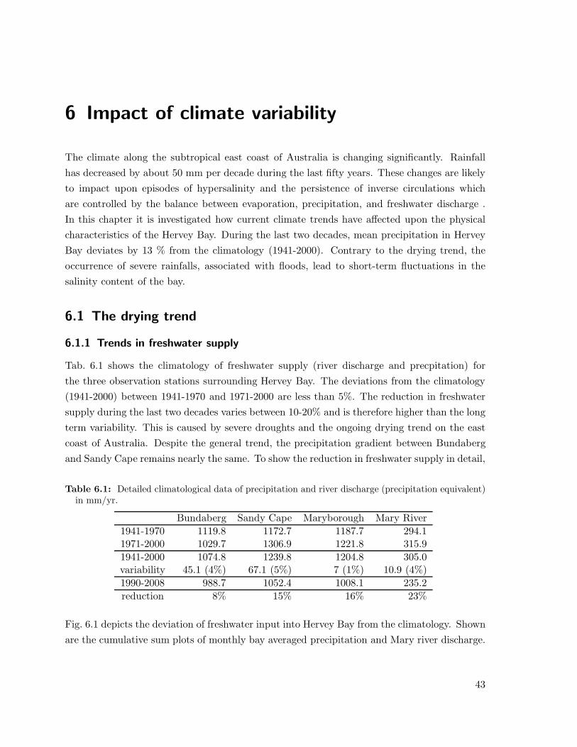
6 Impact of climate variability
The climate along the subtropical east coast of Australia is changing significantly. Rainfall
has decreased by about 50 mm per decade during the last fifty years. These changes are likely
to impact upon episodes of hypersalinity and the persistence of inverse circulations which
are controlled by the balance between evaporation, precipitation, and freshwater discharge .
In this chapter it is investigated how current climate trends have affected upon the physical
characteristics of the Hervey Bay. During the last two decades, mean precipitation in Hervey
Bay deviates by 13 % from the climatology (1941-2000). Contrary to the drying trend, the
occurrence of severe rainfalls, associated with floods, lead to short-term fluctuations in the
salinity content of the bay.
6.1 The drying trend
6.1.1 Trends in freshwater supply
Tab. 6.1 shows the climatology of freshwater supply (river discharge and precpitation) for
the three observation stations surrounding Hervey Bay. The deviations from the climatology
(1941-2000) between 1941-1970 and 1971-2000 are less than 5%. The reduction in freshwater
supply during the last two decades varies between 10-20% and is therefore higher than the long
term variability. This is caused by severe droughts and the ongoing drying trend on the east
coast of Australia. Despite the general trend, the precipitation gradient between Bundaberg
and Sandy Cape remains nearly the same. To show the reduction in freshwater supply in detail,
Table 6.1: Detailed climatological data of precipitation and river discharge (precipitation equivalent)in mm/yr.
Bundaberg Sandy Cape Maryborough Mary River
1941-1970 1119.8 1172.7 1187.7 294.11971-2000 1029.7 1306.9 1221.8 315.9
1941-2000 1074.8 1239.8 1204.8 305.0variability 45.1 (4%) 67.1 (5%) 7 (1%) 10.9 (4%)
1990-2008 988.7 1052.4 1008.1 235.2
reduction 8% 15% 16% 23%
Fig. 6.1 depicts the deviation of freshwater input into Hervey Bay from the climatology. Shown
are the cumulative sum plots of monthly bay averaged precipitation and Mary river discharge.
43

6 Impact of climate variability
Two major events are visible. During 1992 strong rainfalls and river floods occurred, caused
by an El Nino event. The classification into El Nino/La Nina are based on the Oceanic Nino
Index (ONI, [NOAA, 2009]). The floods and rainfalls in 1999-2000 occurred during a La Nina
event. In 1992, the freshwater supply recovered to the climatology. Although the rainfalls in
1999-2000 were significant, they could not replenish the water deficit. Due to long/persistent
droughts, the soil moisture in the catchments were low, thus a certain amount of rainfall
was needed first to recharge soil moisture and ground water, until significant runoff could be
released. The La Nina events 1996 and 2008 show a signature in the river discharge but are
in general of minor importance.
In the following, the numerical model is used to quantify, how this reduction affects Hervey
Bay.
1990 1992 1994 1996 1998 2000 2002 2004 2006 2008−3
−2
−1
0
1
Year
Cum
mul
ativ
e pr
ecip
itatio
n [m
m/y
r]
1990 1992 1994 1996 1998 2000 2002 2004 2006 2008−0.3
−0.2
−0.1
0
0.1
Cum
mul
ativ
e riv
er d
isch
arge
[mm
/yr]
PrecipitationMary River
Figure 6.1: Deviation of freshwater flow into Hervey Bay from the climatology (1941-2000). Shownare the cumulative sum plots of monthly bay averaged precipitation and Mary river discharge. Thegrey bars indicate El Nino/La Nina events. Note that the river discharge has a different scaling toemphasise details.
6.1.2 Hypersalinity and inverse state
The density (Fig. 5.8a) and salinity (Fig. 5.8b) gradient times series clearly show the impact
of the 1999 and 2008 La Nina and also the 1992 El Nino event. Further during the last decade
less frequent reversals of the salinity gradient occurred. To understand the impact of the
drying trend, the days in the year are computed, where the salinity gradient and the density
gradient exceed the critical thresholds. A year is defined from July to June and therefore
the complete southern hemisphere summer is included in one year. The results are shown in
44
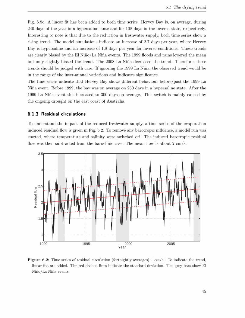
6.1 The drying trend
Fig. 5.8c. A linear fit has been added to both time series. Hervey Bay is, on average, during
240 days of the year in a hypersaline state and for 108 days in the inverse state, respectively.
Interesting to note is that due to the reduction in freshwater supply, both time series show a
rising trend. The model simulations indicate an increase of 2.7 days per year, where Hervey
Bay is hypersaline and an increase of 1.8 days per year for inverse conditions. These trends
are clearly biased by the El Nino/La Nina events. The 1999 floods and rains lowered the mean
but only slightly biased the trend. The 2008 La Nina decreased the trend. Therefore, these
trends should be judged with care. If ignoring the 1999 La Nina, the observed trend would be
in the range of the inter-annual variations and indicates significance.
The time series indicate that Hervey Bay shows different behaviour before/past the 1999 La
Nina event. Before 1999, the bay was on average on 250 days in a hypersaline state. After the
1999 La Nina event this increased to 300 days on average. This switch is mainly caused by
the ongoing drought on the east coast of Australia.
6.1.3 Residual circulations
To understand the impact of the reduced freshwater supply, a time series of the evaporation
induced residual flow is given in Fig. 6.2. To remove any barotropic influence, a model run was
started, where temperature and salinity were switched off. The induced barotropic residual
flow was then subtracted from the baroclinic case. The mean flow is about 2 cm/s.
1990 1995 2000 2005
1
1.5
2
2.5
3
3.5
Year
Res
idua
l flo
w
Figure 6.2: Time series of residual circulation (fortnightly averages) - [cm/s]. To indicate the trend,
linear fits are added. The red dashed lines indicate the standard deviation. The grey bars show El
Nino/La Nina events.
45

6 Impact of climate variability
A closer inspection of the time series shows that the flow is weaker during summer than
during winter. This seems puzzling but the weakening of the evaporation induced residuals
during summer is caused by the EAC.
In Tab. 2.1 the transport of the EAC is given (see also Fig. 2.1). The current is strongest
during summer (18 Sv) and weaker during winter (12 Sv). The EAC induces an anti clockwise
circulation within Hervey Bay. This residual flow is estimated to be in the range of 1-2
cm/s and therefore of the same order as the evaporation induced clockwise flow. Thus during
summer the EAC can slow down the evaporation induced flow. Furthermore, this flow shows
a rising trend. The increase during the simulation period is about 18%. Fig. 6.2 also shows
the standard deviation, which is in the same range as the estimated trend. Thus, during the
two decades of simulations the reduction of freshwater leads to an acceleration of the residual
circulation.
6.1.4 Salinity flux
The model indicates that since 1990, the salinity flux has increased by about 22 % (linear fit in
Fig. 5.10). This corresponds to a rise of approx. 0.9 ton/s during the simulation period. The
mean flux is estimated to be 3.95 ton/s. Again the standard deviation is indicated, which is
now with 4.1 ton/s the fourfold on the trend. Thus, the model indicates a trend, but to show
that this increase is significant, the simulation period has to be at least doubled.
The analysis of the simulations further showed that the annual mean heat content of the bay,
solar heat flux and air temperature remain nearly constant over the whole simulation period.
They are only responsible for the intra-annual variability. The most important factor influ-
encing the rising trend in the salinity gradient/salinity flux is therefore the positive difference
between evaporation and precipitation/river discharge.
6.1.5 Impact of the East Australian Current (EAC)
To quantify the importance of the EAC on the hydrodynamics in Hervey Bay, two additional
experiments were conducted. The aim was to reduce the southward transport of the EAC.
The average transport is approx. 7.1 Sv (Tab. 2.1). In the first experiment, the transport was
reduced to 3.5 Sv and in the second experiment; the EAC was completely switched off. These
modifications were implemented by reducing the background sea surface gradient, causing the
EAC. To preserve the dynamics, the sea surface height anomalies were left unchanged.
The comparison of the numerical results with the measurements from the field trips shows
that the impact on the temperature field was of minor importance. The variations in the
salinity field were noticeable. The impact of the EAC was further visible in the salinity and
the density gradient time series, shown in Fig. 6.3. The EAC acts as low pass filter and
smoothes the salinity and the density differences. By completely switching off the EAC, the
peak values of the salinity and density gradient increased by approx. 10%. Especially from
46

6.2 Short term variability
a)
∂ S
−0.02
0
0.02
b)
Year
∂ S
1990 1993 1996 1999 2002 2005 2008
−0.02
0
0.02
Figure 6.3: a) Time series of density gradient - ∂ρ [kg/m3/km], b) salinity gradient - ∂S [psu/km].Shown are daily averages. The red lines indicate the difference between the simulation and a run,where the EAC was completely switched off. The grey bars indicate El Nino/La Nina events.
2000 onwards, the shut down of the EAC lead to a systematic increase in the salinity and
the density gradient. The simulations further indicate that the interannual variations in flow
strength of the EAC are noticeable, but rather unimportant. The dynamics in Hervey Bay are
a local feature and the EAC causes only a weak modulation. A possible explanation is that
the stream reattaches south of 25°S to the shelf. Further, Break Sea Spit (Fig. 3.1) shields
Hervey Bay from the ocean. In conclusion, the EAC has no direct influence on Hervey Bay,
for instance due to eddy entrainment.
Finally, the southward transport was investigated to detect a possible trend in the volume
transport. The analysis showed that the EAC slightly accelerates, but the trend in the two
decades is less than 1/6 of the standard deviations and thus not significant and can not explain
the increase in salininity flux and residual circulation.
6.2 Short term variability
The IPCC predicts that heavy precipitation events become more frequent over most regions
throughout the 21st century [IPCC, 2007]. This would affect the risk of flash flooding and
urban flooding. Australia’s strongest recent examples were in 1973-74, 1988-89 and May 2009.
In this recent example, within some days, approx. 300 mm, in total, rain was measured along
the Sunshine Coast (Brisbane up to Hervey Bay). This is around one third of the annual mean.
Northern Brisbane had peak values of 330 mm/day. Unfortunately, these data could not be
47

6 Impact of climate variability
compiled into the simulations (due to missing river gauge data). However, Fig. 6.4 shows
times series of the Mary River and Burnett River discharge. Two extreme flooding events are
visible, one in February 1992 and in February 1999. The latter one lead to significant loss of
seagrass in the Great Sandy Strait [Campell and McKenzie, 2004]. Because the peak values of
the Burnett River are only about one sixth of the maximum flow of the Mary River, the main
focus of the short term variability is on the impact of the Mary River.
Year
Riv
er d
isch
arge
1990 1993 1996 1999 2002 2005 20080
2000
4000
6000
8000
Mary River
Burnett River
Figure 6.4: Freshwater discharge of the Mary and Burnett River (1990-2008) in m3/s. The grey barsindicate El Nino/La Nina events.
6.2.1 Catchment area
The catchment area of the Mary River covers 5000 km2. It reaches from 25.2°to 27°S and from
152° to the coast (see Fig. 2.1), thus a stripe of 150×50 km2. The Mary River flows into the
northern region of the Great Sandy Strait draining modified catchment of dryland grazing,
agricultural crops, cleared land, forests and both sewered and unsewered urban development
areas [Rayment and Neil, 1997]. For an average rainfall year, 21% of rainfall is exported as
runoff into the Mary River and 268,000 tonnes of eroded sediments flow into nearshore regions
annually. The river further flushes nitrogen (1.7 kg/ha/y) and phosphorus (0.2 kg/ha/y) into
the Great Sandy Strait passage each year [Schaffelke, 2002].
48

6.2 Short term variability
6.2.2 River discharge statistics
The river discharge time series in Fig. 6.4 are rather spiky. The peak values for the 1992 and
1999 flood reached 7000 m3/s. In Fig. 6.5 the cumulative distribution functions (CDF) for
the Mary and Burnett Rivers are given. The mean flow for the Mary River is 30 m3/s and 10
m3/s for the Burnett River. The Median is 3 m3/s and 0.8 m3/s, respectively, and therefore
only a tenth of the mean. Thus, most of the time both rivers are almost dry. The rare extreme
events shift the mean to higher values. The CDF indicates, that the probability to exceed a
flowrate of 70 m3/s for the Mary river and 30 m3/s for the Burnett River is less than 5%. Fig.
6.4 further indicate that the high flow volumes are strongly linked to El Nino/La Nina events.
1 10 30 100 1000
0.01
0.1
0.5
1
River discharge
CD
F
Mary River
Burnett River
Median
Figure 6.5: Cumulative distribution functions (CDF) of the freshwater discharge (in m3/s) of theMary and Burnett River (1990-2008).The two dashed lines indicate the mean.
6.2.3 Flooding events
In Fig. 6.6 the response of Hevey Bay to flooding events is shown. Plotted are the depth aver-
aged salinity field and a transect in the southern part of the bay, 10 days past the peak flow of
the Mary River. The river discharge associated with these flooding events is 7100 m3/s (1992),
6700 m3/s (1999) and 900 m3/s (2008), see also Tab. 6.2. The peak value of 900 m3/s seems
rather low, compared to the 1992 event. However, the 2008 flood was preconditioned by three
750 m3/s peaks (in the 40 days before the flood) and puts it therefore in a comparable range to
the 1992 event. Fig. 6.6 indicates, that the outflow of the freshwater is restricted to a narrow
region along the western coast. The transects for 1992 and 1999 further indicate a pronounced
frontal structure (horizontal and vertical). Beside this narrow coastal freshwater strip, the
whole bay is mainly unaffected by the flood. Although the river discharges for the 1992 and
49

6 Impact of climate variability
Table 6.2: Atmospheric condition and river discharge for three flood events.
Year River discharge Wind direction Wind speed
1992 7100 m3/s SE 6 m/s1999 6700 m3/s S 8 m/s2008 900 m3/s SE 3 m/s
1999 flood are comparable, the transects in Fig. 6.6 show a different behaviour. Whereas in
1992 the bay has a nearly uniform salinity distribution, strong salinity stratifications are visible
for 1999. These differences are mainly caused by the location of the strong rainfalls. For 1992,
they occurred mostly in the southern parts of the Mary River catchments combined with minor
precipitation in Hervey Bay. For 1999, the rainfalls were uniformly distributed over Hervey
Bay and the catchments. Thus, due to the heavy precipitation, a freshening of the surface
layer is visible (Fig. 6.6b) and thus explaining the vertical salinity stratification. This further
explains the greater width of the river plume. Both events are assisted by strong southerly
winds. Hence, a northward flow-through in the Great Sandy Strait prevents an outflow of the
Mary River discharge into the southern region of the Strait. This high flow-through further
pushes the riverine water quite effectively into the bay. This is not the case for the 2008 floods.
Due to the light winds, the fresh water remains in the northern part of the Strait. Moreover,
the saline water in the bay acts as a salt barrier, which prevents the transport of the riverine
fresh water into Hervey Bay. Further, the low river discharge leads only to a weak coastal
plume on the western shore (Fig. 6.6c).
(a)
−25.2
−24.8
(b)
−25.2
−24.8
(c)
152.6 153
−25.2
−24.8
35 35.2 35.4 35.6 35.8 36 36.2 36.4 36.6
−15
−5
−15
−5
152.6 153.0
−15
−5
Figure 6.6: Depth averaged salinity (in psu) for a) 4 Mar. 1992, b) 20 Feb. 1999 and c) 23 Mar.2008. In the left column the salinity transects along the red lines are shown.
50

6.2 Short term variability
6.2.4 The flood of 1999
In the following, the 1999 flood event (February 1999) [Campell and McKenzie, 2004] is used
to estimate typical exchange time scales associated with high riverine flow, and also a time
which is needed for Hervey Bay to recover to a “normal state”.
Two experiments are conducted. In the first one, called the flood run (FR), the river discharge,
atmospheric boundary conditions and open ocean boundary conditions are prescribed using
the forcing given in Sec. 2.2. At the same time, a neutral tracer with a concentration of 100
units was released into the river. In the second experiment, the control run (CR), the high
river discharge due to the flood is completely switched off. Both experiments start at the 1.
February 1999 and run for three months. Fig. 6.7 shows the impact of the 1999 flood event.
de
f
a)
152.6 153.0
−25.2
−24.8
0
2000
4000
6000
Riv
er d
isch
arge
b)
Feb Mar Apr May−0.03
−0.02
−0.01
0
∂ S
c)
20
25
30
35
Sal
inity
d)
10
20
30
40
Tra
cer
30
35S
alin
itye)
0
10
20
Tra
cer
30
35
Sal
inity
f)
Feb Mar Apr May0
20
Tra
cer
Figure 6.7: a) position of three virtual measurement stations to showing the impact of the 1999flood, b) river discharge in m3/s, c) salinity gradient ∂S in psu/km (see also Fig. 5.8). The bluecurve represents the flood run (FR) and the red curve the control run (CR). Pictures d-f shows thesalinity at the three stations d-f. The green curve indicates the tracer concentration.
The peak river discharge is approx. 7600 m3/s at the afternoon of the 9 February. In the
beginning of March a second minor flood occurred with a peak flow of 800 m3/s. In Fig. 6.7c
the impact of the flood on the salinity gradient is visible. The transect is positioned close to
station f. The minimum gradient has a delay of 6 days compared to the flood peak. This
corresponds to a plume velocity of 10 cm/s. Taking the wind conditions for this event into
account (Tab. 6.2), clearly shows, that the plume is advected along the western shore, due to
the wind induced currents (Fig. 4.2). Fig Fig. 6.7c further indicates that, although the salinity
gradient shows a significant minimum, Hervey Bay completely recovers to the undisturbed
state (CR) within two months.
51
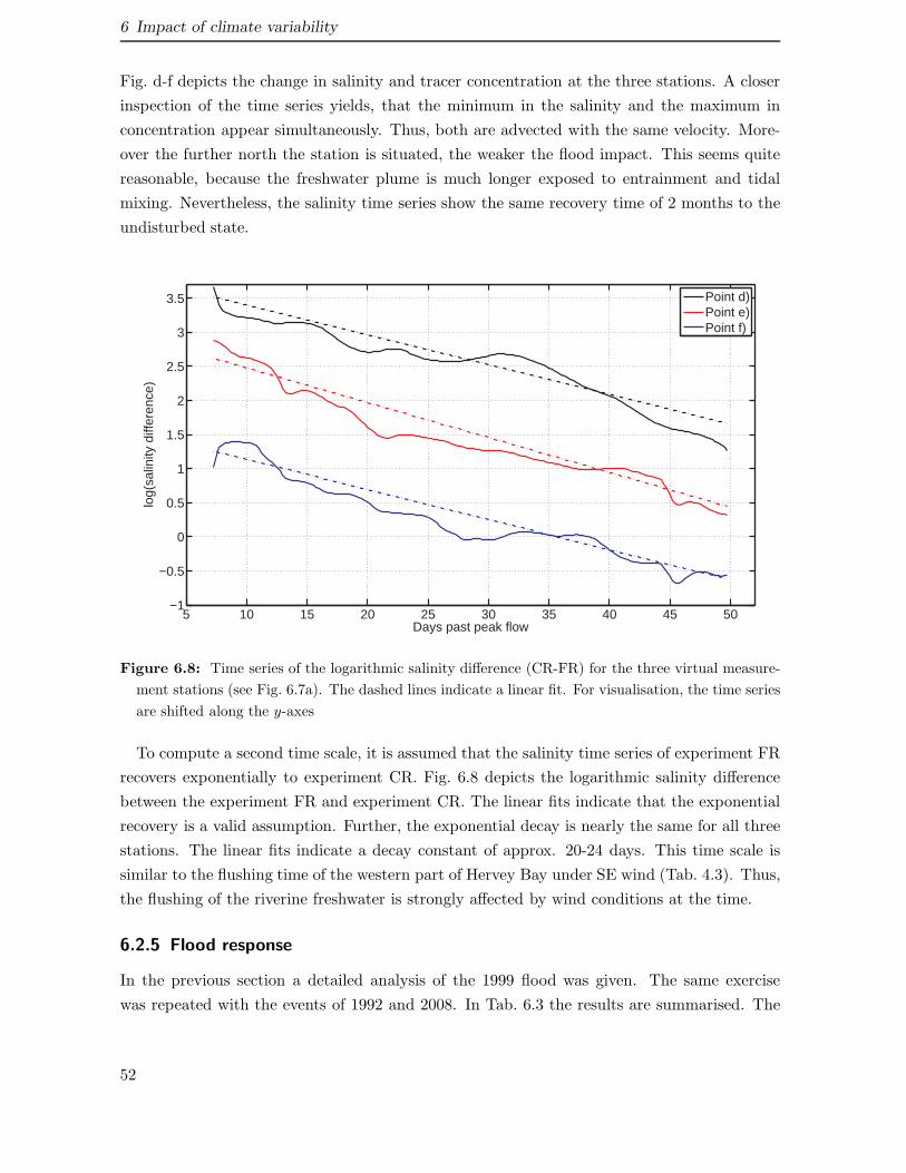
6 Impact of climate variability
Fig. d-f depicts the change in salinity and tracer concentration at the three stations. A closer
inspection of the time series yields, that the minimum in the salinity and the maximum in
concentration appear simultaneously. Thus, both are advected with the same velocity. More-
over the further north the station is situated, the weaker the flood impact. This seems quite
reasonable, because the freshwater plume is much longer exposed to entrainment and tidal
mixing. Nevertheless, the salinity time series show the same recovery time of 2 months to the
undisturbed state.
5 10 15 20 25 30 35 40 45 50−1
−0.5
0
0.5
1
1.5
2
2.5
3
3.5
Days past peak flow
log(
salin
ity d
iffer
ence
)
Point d)Point e)Point f)
Figure 6.8: Time series of the logarithmic salinity difference (CR-FR) for the three virtual measure-
ment stations (see Fig. 6.7a). The dashed lines indicate a linear fit. For visualisation, the time series
are shifted along the y-axes
To compute a second time scale, it is assumed that the salinity time series of experiment FR
recovers exponentially to experiment CR. Fig. 6.8 depicts the logarithmic salinity difference
between the experiment FR and experiment CR. The linear fits indicate that the exponential
recovery is a valid assumption. Further, the exponential decay is nearly the same for all three
stations. The linear fits indicate a decay constant of approx. 20-24 days. This time scale is
similar to the flushing time of the western part of Hervey Bay under SE wind (Tab. 4.3). Thus,
the flushing of the riverine freshwater is strongly affected by wind conditions at the time.
6.2.5 Flood response
In the previous section a detailed analysis of the 1999 flood was given. The same exercise
was repeated with the events of 1992 and 2008. In Tab. 6.3 the results are summarised. The
52

6.2 Short term variability
simulation indicates, that although the flood related river discharges differs significantly, the
recovery times vary only slightly. For all three events, Hervey Bay shows a decay rate of the
disturbance, of approx. 22 days. This recovery time scale to the experiment CR is seen in the
salinity and in the salinity gradient. The simulations further indicate, that the flood response
is closely related to the wind induced residual circulations. The exponential decay with approx.
22 days, can also be seen in the residence time for SE wind (Tab. 4.3).
Table 6.3: Exponential recovery time for the three flood events in days. The salinity recovery is
averaged over the three stations. The salinity gradient ∂S is computed along the transect indicated
in Fig. 3.1. For 2008, this measure could not be computed.
Year River discharge salinity recovery ∂S recovery
1992 7100 m3/s 26 d 20 d
1999 6700 m3/s 22 d 18 d
2008 900 m3/s 20 d -
53

7 Gravity currents
7.1 Release of gravity currents
The density gradient time series in Fig. 5.8a show, that the density at the shore is higher
than on the shelf. This leads to the establishment of an inverse circulation. Because the
positive density gradient is a gravitational unstable state and therefore gravity induced flows
are triggered. This flow of dense water originating from cooling, evaporation, or salinisation
on the shelf, spills over the shelf edge and can develop as near-bottom gravity current or
an intermediate-depth intrusion. Quite often, it is difficult to observe them in nature due
to their intermittent character. It is worth mentioning that until now no observations of
the gravity flows in Hervey Bay are available. The main research focus was on Hervey Bay
itself; therefore, no field measurements were taken on the northern shelf. Middleton et al.
[1994] lacked observational evidence in support of their hypothesis that Hervey Bay potentially
exports high salinity water formed through a combination of heat loss, high evaporation, and
weak freshwater input in shallow regions of the bay. ... Thus, a second hypothesis is that
the high nutrient, low-oxygen waters that constitute the anomalous water masses observed at
both the Sandy Cape and Double Island Point sections consist partly of cooler, saltier ’winter
mangrove waters’ exported both north and south of the Great Sandy Strait on each flood and ebb
tide. The exported waters would subsequently sink off the continental shelf to their own density
level, progressively mixing with ambient waters... Thus the common assumption was, that tidal
flushing would lead to constant export of this dense water to the continental shelf. Further due
to its low aspect ratio and therefore the lack in supporting high density gradients, significant
gravity currents ( [Tomczak, 1985; Lennon et al. , 1987; de Silva Samarasinghe, 1998] were not
expected.
Fig. 7.1a shows such a flow event in June-July 1995. The density within Hervey Bay reaches
values of greater than σt=26.2 kg/m3, which is equivalent to a depth of approx. 300 m. During
its way down the shelf, the plume is channelled in the Mary River Canyon, to finally reach a
depth of 200 m.
7.1.1 Formation
To describe the four different stages in the development of the gravity flows, the classification
54

7.1 Release of gravity currents
a)
26.2
25.2
25
152 152.5 153
−25
−24.8
−24.6
−24.4
−24.2
−24
17
20
b)
152 152.5 153
−25
−24.8
−24.6
−24.4
−24.2
−24
c)
35.6
36
152 152.5 153
−25
−24.8
−24.6
−24.4
−24.2
−24
Distance [km]
Dep
th [m
]
d)
0 50 100−200
−150
−100
−50
0
24.5 25 25.5 26
Figure 7.1: a)bottom density σt [kg/m3] on the 28 July 1995, b) bottom temperature - [C], c) bottom
salinity - [psu] and d) σ-density along the black line in b) [kg/m3]. The thick dashed lines in a,b and
c are the 40 m, 100 m and 300 m depth isolines.
proposed in Shapiro and Hill [2003] is used. The pre-conditioning is the stage when dense
water accumulates on the shelf and a density front is formed. The short active stage corre-
sponds to the period when the leading edge of the dense water accelerates down-slope. The
main stage relates to a quasi-steady flow with a noticeable down-slope component. These two
stages can also be combined in a down-slope propagation stage. The final stage is reached when
the water spreads isopycnically off the slope, but traces of the cascade may still be detected
by inclined isopycnals over the slope.
7.1.2 Pre-conditioning
To trigger gravity currents in Hervey Bay, three conditions are necessary. First, the density
gradient has to exceed 0.008 kg/m3/km. This is a rather moderate gradient and the same
as the threshold to define inverse circulations. The second condition, which is necessary, is
that the SST in Hervey Bay has to drop below 20°C. This condition is mostly fulfilled during
June/July. The salinity gradient is of minor importance. The dependence on the SST indicates,
that Hervey Bay has a temperature driven cascade [Shapiro and Hill, 2003], with a response
55

7 Gravity currents
to surface cooling assisted by advection of salinity. The third mechanism is the tidal forcing.
The initialisation of the plume coincides with the occurrence of neap tide. During this time
tidal mixing is sufficiently reduced and a two layered flow structure can develop.
Wind forcing is not directly involved into the triggering of the plumes. It is only important
to maintain the gradients across the shelf. The wind forcing is important to restrict the path
of the plume between Breaksea Spit and Lady Elliot Island (see Fig. 3.1). Such an event
is shown in Fig. 7.1. In the northwestern part of the shelf, water of low density and higher
temperature is situated. This acts as an effective barrier for a northward flow of the plume.
Hence, the whole flow is directed into the Mary River Canyon. This is a typical situation
during northeasterly wind. Relative warm water from the southern part of the Great Barrier
Reef is pushed southwards onto the northern shelf of Hervey Bay. Further, the saline water
from the northern shelf is advected into the bay. This mechanism supports the intensification
of the flow but is not necessary to actually release the plume.
7.1.3 Down-slope propagation
The flow of the plume is mainly controlled by the steepest decent into the Mary River Canyon.
Therefore, topography suppresses the effects of earth rotation until the plume reaches the
100 m depth isoline. Although the flow is disturbed by the bathymetry, a good estimate to
compute the frontal velocity uNof is given by Nof [1983].
uNof = g′tanα
fwith g′ =
∆ρ
ρ0(7.1)
where g′ is the reduced gravity within the plume, f is the Coriolis frequency and α is the
bottom slope. To compute this theoretical velocity f is taken to be 3·10−5 s−1 and α is
estimated with 0.0016. To compute the reduced gravity, the density gradient (see Fig. 5.8a)
is used. The transect to calculate the gradient is aligned with the flow path of the plume and
has a length of 60 km. Using a density gradient of 0.008 kg/m3/km, equivalent to a density
difference of 0.5 kg/m3, leads to a maximum frontal speed of 0.25 m/s. This velocity is also
seen in the simulations. The average flow velocity in the steady state is approx. 5-7 cm/s.
Inspection of the time series shows that the plume front passes the 100 m isolines approx. 5-8
days past neap tide. This can be explained by simple geometry. The gravity current needs
on average 6 days to travel 150 km, which is approx. the shelf width. Therefore, the reduced
mixing during neap tide is necessary to trigger the release of the plumes.
If the plume has passed the 60 m isoline, the slope of the shelf nearly doubles (see Fig. 7.1d).
According to Eq. (7.1) this would cause a doubling of the frontal speed, which is not seen in
the simulations. Due to dispersion and intrusion, the density gradient across the plumes starts
to weaken, reduces therefore g′ and balances thus the change in bottom slope.
After passing the 60-80 m isoline, the plume is no longer restricted in its flow path by the
56

7.2 Impact of freshwater reduction
bathymetry. Using the distribution of salinity (see Fig. 7.1c), the deviations of the front to the
left are visible. Hence, there exists a balance of Coriolisforce and the component of gravity in
the cross-flow direction. The angle θ at which the current is deflected down slope by friction
can be estimated [Bowers and Lennon, 1987] as
tan θ =(ks + kb) u
f h(7.2)
where kb is the bottom friction coefficient, ks is an interfacial friction coefficient, uNof the
frontal speed and h the thickness of the plume. The only unknown here is the interfacial
friction ks. Using kb=0.0025, u = uNof , f=3·10−5 s−1, h=10 m (Fig. 7.1d) and estimating
θ=25°, yields ks=0.002, which is of the same order as the bottom friction coefficient. This is
in broad agreement with observations [Pederson, 1980].
7.1.4 Fate of the plume
After the head of the cascading plume has reached its equilibrium density level (which can be up
to 280 m), it detaches from the bottom, intruding into the ambient water as an isopycnal layer.
Heat and salt exchange with the surrounding water causes transformation of cascading water
and levelling salinity and temperature differences. The whole mixing process is enhanced by
the strong ambient currents (EAC) which additionally facilitates distant spreading of cascading
water from the source area. This was also observed by Tomczak [1985].
7.2 Impact of freshwater reduction
To quantify the impact of the freshwater reduction it is first necessary to define an outer
envelope for the gravity current. For Hervey Bay the isopycnal surface σt = 25.4 has been
taken for this purpose. This density contour is equivalent to depths of approx. 150-180 m. A
gravity flow starts if the σt = 25.4 contour crosses the 100 m depth line between Lady Elliot
Island and Break Sea Spit (Fig. 3.1). The same argument holds to define the termination
of the flow. During the occurrence of the gravity flow, the duration and the total volume,
transported down the shelf, is computed. Fig. 7.2 shows the duration and the volume flow for
each year. The gravity flows occur only once a year, mostly during June/July.
The average duration is 29 days (Fig. 7.2a) but can range from one week up to two months.
The average water transport associated with the plumes is comparable with the volume of
Hervey Bay. Peak values of twice the bay volume are observed.
It is rather difficult to identify a possible trend. It seems that there is an increase in duration
and magnitude of these outflow events, especially when comparing the first 10 years with the
last decade. Given the noisy signal, a firm conclusion cannot be given at this time.
57

7 Gravity currents
1990 1995 2000 20050
10
20
30
40
50
60
Flo
w d
urat
ion
in d
ays
Year
(a)
1990 1995 2000 20050
0.5
1
1.5
2
2.5
Nor
mal
ised
flow
vol
ume
Year
(b)
Figure 7.2: a) duration of gravity flows [days] and b) down shelf transport normalised by the volume
of Hervey Bay. The gravity flows are tracked between Lady Elliot Island and Break Sea Spit. A
gravity plume is defined to be bound by the σt=25.4 [kg/m3] isoline. This is equivalent to a depth of
approx. 150 m. The duration and the down shelf transport are only counted past the 100 m depth
isoline.
58
8 Conclusion
In this study the ocean model COHERENS has been applied to compute, amongst the usual
hydrodynamic variables, the temperature and salinity distribution within Hervey Bay, Aus-
tralia. A model validation and calibration has been carried out using recent in-situ field,
satellite AVHRR SST data, and pan evaporation measurements. Observations and model re-
sults show that the bay is in parts vertically well mixed throughout the year. The absence of
longer lasting stratification is caused by the tidal regime within Hervey Bay. The tidal range
can exceed 3.5 m. Due to the tidally induced bottom shear, the whole water column is con-
trolled by the bottom Ekman layer most of the time. Therefore only horizontal fronts appear.
Only during a short time around neap tide, a temperature induced stratification can develop
and the bottom to surface density difference can exceed 0.3 kg/m3. The dominant mechanism
forcing residual circulations in the bay is provided by the Trade winds from the east, with a
northern component in autumn and winter, and a southern component in spring and summer.
The wind-induced currents are in the range of 5-10 cm/s. The contribution of the tides to the
residual currents is negligible. Hence, the tides are only responsible for mixing.
To quantify the impact of the residual circulations on the water exchange of Hervey Bay with
the northern shelf/open ocean, the concept of flushing time and residence time was introduced.
Because both measures are defined in different frameworks (Eulerian/Lagrangian), different
aspects of the water exchange could be investigated. The weak tidal residual currents lead to
flushing/residence times of approx. 3 months. During SE wind conditions (Trade winds), the
water exchange times were in the range of 20 days. The clockwise circulation pattern yield
faster flushing times for the western part of the bay compared to the eastern part. During NE
wind, the exchange time scales are comparable to SE wind, only the pattern changed. Due to
the large-scale circulation cell, that connects Hervey Bay with the northern shelf (during NE
wind), the central part of the bay showed the fastest response. This outflow of Hervey Bay
water through the central part of the bay could also be observed in the temperature pattern
of the September 2004 field trip.
Climatological data indicate that Hervey Bay is a hypersaline bay that also exhibits features
of an inverse estuary, due to the high evaporation rate of approximately 2 m/year, a low pre-
cipitation rate of less than 1 m/year and an on average almost absent freshwater input from
the two rivers that drain into the bay. As in other inverse estuaries, the annual mean salinity
increases towards the shore to form a nearly persistent salinity gradient. The region therefore
acts as an effective source of salt accumulation and injection into the open ocean. The high
59

8 Conclusion
evaporation is leading to a loss of freshwater and increases salinity within the bay. The aver-
age salinity flux into the open ocean is estimated to be about 4.0 tons/s. This study showed
that this transport is mainly caused by advective transport, whereas the diffusive transport
is on average three orders of magnitude smaller. Furthermore, the evaporation loss and the
accumulation of salt within the bay leads to evaporation induced residual circulation of the
order of 2-4 cm/s.
The numerical modelling that was carried out made it possible to understand in detail, how
the actual drying trend on the east coast of Australia impacts on the hydrodynamics of Her-
vey Bay. During the last two decades the drying trend has manifested itself in a reduction of
precipitation by 13 % and a reduction in river discharge by 23 %. This is much higher than the
long-term variability suggested and shows the impact of severe droughts during the last two
decades. As a direct consequence, hypersaline/inverse conditions are more persistent but they
did not increase in magnitude. Further the baroclinic residual circulation accelerated by 18 %
due to the disturbance of the evaporation/precipitation ratio. The signal visible in the salinity
flux shows an increase by 22 % but the annual variations are higher than the trend. Thus,
longer simulation times should give more confidence. Due to the lack in boundary conditions
and forcing data, the simulations could only run from 1990 onward.
Due to the inverse conditions and thus gravitational unstable conditions, gravity currents are
released. These flows have a duration of approx. 30 days and are associated with a volume
transport comparable to the total volume of Hervey Bay. The signature of these outflow events
can be found up to depths of 280 m. A clear signal due to the reduced freshwater supply is
not visible, but the model indicates a slight increase in volume transport and duration.
Despite the drying trend, two major flood events occurred in Hervey Bay 1992 and 1999. The
riverine freshwater flow is restricted to an approx. 10-15 km narrow band along the western
shore of the bay. The simulations yield that essentially most of Hervey Bay is unaffected by the
floods. The recovery time, to an undisturbed state, follows an exponential law with a typical
decay time of 22 days. This time scale is similar to a flushing time for the western bay due to
SE winds. Thus, the export of the freshwater is strongly affected by the wind conditions at
the time of the event.
Due to the lack of validation data for biology/chemistry, only the impact on the hydrodynam-
ics could be investigated. Therefore the understanding of the influence of the drying trend on
the local flora/fauna would be of great interest but is at this stage of rather speculative nature.
Although the simulation time span is with 18 years rather short and is biased by severe El
Nino/La Nina events, the simulations demonstrate that recent climate trends impacted on
physical marine conditions in subtropical regions of eastern Australia and are likely to do so
in the future if current climate trends, especially drying, are to continue.
60
A Particle tracking schemes
A.1 Introduction
The behaviour of particles in turbulent flows has been studied for many years, ranging for me-
teorology [Brickman and Smith, 2001; Cencini et al. , 2006] to ocean dynamics [North et al. ,
2006; Visser, 1997, 2008]. Extensive literature exists on the treatment of Lagrangian trajec-
tories, ranging from highly idealised flows to situations as complex as the unstable convective
boundary layer or frontal zones. The level of understanding of these types of models has
greatly increased over the years. In the same time the need to predict the transport of parti-
cles, pollutants, or biological species has resulted in a rapid rise in the use of these numerical
models.
The random walk simulation model enables the observation of phenomena on scales much
smaller than the grid size, as well as the tracing of the movement of individual particles,
thereby describing the natural processes more accurately. Furthermore, information on inte-
grated properties like: residence/settling time or individual tracks are easily extracted from
the simulations. Concentrations of particles can be directly calculated from the spatial posi-
tions of the particles and, more importantly, when and where required. Additionally, errors
due to numerical diffusion inherent in methods such as finite differences or finite elements,
are avoided, particularly in areas where high concentration gradients exist, such as close to
point sources or frontal zones. Although there are methods to circumvent these difficulties
[Chung, 2002], their implementation is problematic in complex geometries, where it is difficult
to control the potential sources of error.
The development of particle tracking methods (or random walk / random dispersion methods)
started by tracking neutrally buoyant particles, i.e. water parcels [Maier-Reimer and Sundermann,
1982; Visser, 1997]. Hunter et al. [1993] and Visser [1997] also showed that due to the high
spatial variability of turbulence, the tracking algorithms need special modification to avoid
numerical artefacts. In recent years, a catalogue of test cases was developed to compare
the performance of tracking schemes but also to validate the models [Brickman and Smith,
2001; Deleersnijder et al. , 2006a; Spivakovskaya et al. , 2007]. Deleersnijder et al. [2006a]
extended the test catalogue to particles that have a finite sinking velocity. By this, particle
tracking schemes dealing with sediment or buoyant particles could be validated against an ana-
lytical solution. The random walk schemes for modelling suspended particulate matter (SPM)
dynamics are quite attractive, because they give a straightforward physical interpretation of
61
A Particle tracking schemes
the processes and automatically account for suspension and bed load.
Because of these advantages, Lagrangian schemes have also become more common in the SPM
modelling community [Charles et al. , 2008; Krestenitis et al. , 2007; Rolinski et al. , 2005].
Nevertheless most of these models used only small number of particles O(104). Nowadays
with easy access to high performance computer clusters, the tracking of individual particles
can be parallelised with high efficiency and therefore makes huge particle numbers feasible
[Charles et al. , 2008]. This means to deal with particles in the order of > 107. This is still
negligible, by realising that a bucket of muddy water contains more individual particles, com-
pared to the ability of state of the art Lagrangian schemes. Nonetheless increasing the number
of particles leads to a better statistical description and makes the answers, a Lagrangian model
can give, more reliable.
A.2 The Lagrangian model
Dealing with concentration fields (SPM, pollutants, biology, etc.), the time evolution of these
fields is usually formulated as partial differential equations (PDEs) in an Eulerian framework.
∂tC = −∇ · (u C − K · ∇C)
∇ · u = 0(A.1)
The first equation is an advection-diffusion equation for the concentration field C of a passive
tracer, that is coupled to a 3D velocity field u, that shall be divergence free. The diffusivity
tensor K is symmetric and positive definite. In the following only diagonal diffusivity tensors
are considered
K =
KH 0 0
0 KH 0
0 0 KZ
(A.2)
where KH is the horizontal and KZ the vertical diffusivity. Hence, the three spatial dimensions
are decoupled. Instead of solving the PDE, one can transform the whole solution process
into the solution of a system of stochastic differential equations (SDEs) also called Langevin
equations. The basic idea is to interpret the concentration field C(x, t) as a transition density
field and reinterpret Equation (A.1) as a Fokker-Planck equation, i.e. a deterministic PDE
with regard to transition density functions. This can be solved by the following system of
SDEs defined in the Ito sense [Arnold, 1974]:
dX(t) = (u+ ∇ ·K)dt +√
2K dW(t) (A.3)
Here X(t) is the position vector of the particles and dW(t) is a Wiener noise increment with
the following properties. W(t) is a Gaussian process with independent increments for which
62

A.2 The Lagrangian model
holds
〈W(t)〉 = 0 ; Std (W(t) − W(s)) =√
|t− s|I (A.4)
where I is the identity matrix. Therefore the noise process has a vanishing mean 〈·〉, its stan-
dard deviation scales as√dt and the increments are uncorrelated.
The first term on the right hand side of Equation (A.3) represents the deterministic part,
whereas the second term is the stochastic term. In the case of vanishing turbulent diffusiv-
ity, the system of equations reduces to a system of ordinary differential equations (ODEs).
Because the ocean is a turbulent environment, turbulent diffusion has to be included. This
is incorporated via the stochastic term. The particles experience a random displacement due
to eddies of average size√
2Kdt. Because the turbulent diffusivity K = K(x, t) is spatially
highly variable, the term ∇ ·K needs to be added to the deterministic part. This corrects for
an artificial noise induced drift [Hunter et al. , 1993; Visser, 1997].
A.2.1 Numerical approximation
Because the diffusivity tensor is diagonal, the three spatial directions can be treated separately
in developing a numerical approximation to the 3D Langevin equation. Focussing for simplicity
on the vertical dimension the following equation needs to be discretised.
dZ(t) = (w + ∂zKZ(z)) dt +√
2KZ(z) dW (t) (A.5)
This equation can further be simplified to
dZ(t) = a(z) dt + b(z) dW (t) (A.6)
where a = w + ∂zKZ(z), represents the deterministic part and b =√
2KZ(z) is the stochastic
part. Again Eq. (A.6) and (A.5) are only valid in the Ito interpretation [Arnold, 1974].
Instead of writing Equation (A.6) in differential form, it is also common to use the integral
representation
Zt = Z0 +
∫ t
0a(Zs) ds +
∫ t
0b(Zs) dWs (A.7)
A straightforward translation of Equation (A.6) into a numerical scheme, is simply to replace dt
by ∆t and dW by ∆W . This is equivalent to assuming that a(Zs) and b(Zs) in Equation (A.7)
are constant and can be taken out of the integrals. Therefore, the lowest order approximation
reads as
Zn+1 = Zn + a ∆t + b ∆Wn (A.8)
This is also known as Euler scheme. In the following, this approximation is named EULER.
This scheme is commonly used [Brickman and Smith, 2001; North et al. , 2006; Spivakovskaya et al. ,
2007; Visser, 1997]. Although this is a straightforward approach, some difficulties arise in the
63

A Particle tracking schemes
case of SDEs. To define the accuracy or order of convergence for stochastic scheme two cases
have to be distinguish. For SDEs the order of convergence is separated into weak and strong
[Arnold, 1974; Kloeden and Platen, 1992]. A method is said to have weak/strong order of
convergence of γ if there exists a constant Λ such that
|〈p(Zn)〉 − 〈p(Z(τ))〉| ≤ Λ ∆tγ : weak
〈|Zn − Z(τ)|〉 ≤ Λ ∆tγ : strong(A.9)
for any fixed τ = n∆t ∈ [0, T ] and ∆t sufficiently small. Zn represents the true solution and
Z(τ) is the approximation. p(·) is an arbitrary function (in most cases a probability density
function). The weak criterion asks for the difference in a distribution, whereas the strong
criterion accounts for the difference in the trajectory.
As discussed after Equation (A.4) the increment ∆W scales as√
∆t, hence the whole EULER
scheme is only of order√
∆t in the strong convergence. Since we are interested in the time
evolution of a sediment distribution rather than individual trajectories of single sand grains,
the weak convergence is used. In this case the EULER schemes is or order ∆t in the weak
sense.
To develop higher order schemes, that have a higher accuracy in the strong definition, the as-
sumption that a(Zs) and b(Zs) in Equation (A.7) are constant is not valid any more. Using the
appropriate Taylor approximation for the integrals, see e.g. Arnold [1974]; Kloeden and Platen
[1992], the next higher order approximation reads as
Zn+1 = Zn + a ∆t + b ∆Wn +1
2bb′[
(∆Wn)2 − ∆t]
(A.10)
where b′ is the spatial derivative. This is also known as the MILSTEIN scheme. This scheme
is of order ∆t in the weak and strong convergence. Additional accuracy is gained by including
information of the derivative of the noise term b. If this scheme is used in numerical algorithms,
the term bb′ can cause problems due to round off errors. To avoid this, a symmetry property
of Equation (A.6) can be used. By replacing b again by√
2KZ(z) and computing the term
bb′ explicitly it turns out that it is equal to ∂zKZ(z). After some rewriting, the schemes read
as follows
Zn+1 = Zn + w∆t + ∂zK ∆t +√
2K∆W : EULER
Zn+1 = Zn + w∆t + ∂zK(∆W )2+∆t
2 +√
2K∆W : MILSTEIN(A.11)
As stated above the EULER scheme is commonly used, but it is easily appreciated that a
higher accuracy is gained here by a simple multiplication with ∆W · ∆W and one addition.
There are no approximations involved and the extra computational cost is negligible.
To further improve the accuracy of the numerical schemes, more terms in the Taylor approxi-
mations have to be included [Kloeden and Platen, 1992]. Due to the slow convergence of the
64

A.2 The Lagrangian model
numerical schemes for SDEs, the extra computational costs are so far prohibitive. Therefore,
a multi step scheme is proposed, similar to Runge-Kutta schemes for ODEs.
Zn+1 = Zn +1
2
(
a(Z) + a)
∆t + b ∆Wn (A.12)
with
Z = Zn + a∆t + b ∆Wn (A.13)
Equation (A.12) is a stochastic version of the trapezoidal method also known as HEUN
scheme. Note that the predictor step (A.13) is only applied to the deterministic part, the
stochastic part is not corrected to keep the numerical approximation consitent with Eq. A.6
[Kloeden and Platen, 1992]. The HEUN scheme, like the MILSTEIN scheme, is of order ∆t
in the strong and weak convergence.
At this stage, the question might arise, why three algorithms are presented with the same
accuracy. All three algorithms should behave identical in predicting the time evolution of an
initial concentration, because they have the same order of convergence. Assume the limit of
vanishing diffusivity, here the MILSTEIN scheme becomes identical to the EULER scheme.
This is not the case for the HEUN scheme. Due to the predictor-corrector step, the accuracy
is higher. Therefore, in the case of advection-dominated problems, differences will be visible.
This should not be the case if diffusion dominates. However, especially Sec. A.3.3 will show the
limitation of the EULER scheme. Moreover, near boundaries, the proper approximations of
the particle trajectories become important to resolve for instance the bottom boundary layer.
A.2.2 Boundary conditions
The treatment of boundary conditions is always a critical issue in ocean modelling, especially
in coastal regions. The moving sea surface, the sea bottom and lateral boundaries like islands
or beaches have to be considered appropriately. E.g., in the framework of PDEs the sea
surface is an impermeable boundary and a no flux condition is normally imposed (at least for
suspended particulate matter). This no flux condition can be easily violated by overshooting of
the trajectories of simulated particles, due to either too large time steps or the random nature
of the stochastic increment ∆W . This can lead to a crossing of the boundary. To correct this,
a straightforward approach would look like this: When a particle crosses the boundary (due to
a too large random displacement), it is simply reflected back into the domain by the amount
it penetrates into the boundary domain. It would be advantageous in general to minimise the
number of particles that crosses the boundaries in the first place. The first solution that comes
to mind is to reduce the time step of the particle displacement. Nevertheless, this would also
lead to additional computation time in ’open water’. A more expensive method is the use of
a higher-order numerical scheme. This may perhaps not completely prevent the crossing from
happening, but it will at least reduce the number of times that it does occur. This was also
65

A Particle tracking schemes
mentioned by Stijnen et al. [2006].
In the following all boundaries are treated as reflective boundaries (no flux condition), if not
stated otherwise.
A.3 Idealised test cases
In the following section two simple 1-D test cases are described and a 2-D test is considered.
Because the equations which need to be solved are SDEs, special care is taken for the stochas-
tic increment ∆W . A state of the art random number generator computes the increments:
the Mersenne Twister [Matsumoto et al. , 1998]. This generator produces uniform random
numbers in the interval [0, 1]. Because the particle numbers are quite large, standard gener-
ators are limited by their periodicity. Moreover the Mersenne Twister produces uncorrelated
random numbers in higher dimensions. These random numbers are transformed to Gaussian
random numbers by the Box-Muller algorithm [Press et al. , 1986].
A.3.1 1-D diffusion
Firstly, the numerical algorithms are applied to a diffusion test in a bounded region. This can
be visualised as an one dimensional water column that is bounded by the sea surface and the sea
floor. The model is discussed in detail in Deleersnijder et al. [2006a] or Spivakovskaya et al.
[2007]. The governing PDE for this case is written as
∂C
∂t=
∂
∂z
(
KZ(z)∂C
∂z
)
(A.14)
This describes a simple diffusion equation. The diffusivity KZ(z) has the following form
KZ(z) = 6 z (1 − z) (A.15)
This parabolic profile is a good approximation of the diffusivity profile in the upper mixed layer,
but it is also a good description for a shallow, well-mixed, coastal region [Burchard et al. , 1998;
Warner et al. , 2005]. For simplicity, time dependence is not considered. The boundary (BC)
and initial conditions (IC) are
BC:
[
KZ(z)∂C
∂z
]
z=0,1= 0 ; IC: C(0, z) = δ(z − z0) (A.16)
i.e. “no flux” boundary conditions are imposed at the boundaries of the normalised domain
[0, 1]. The initial condition is a delta like concentration peak. The Langevin equation for the
particle trajectories takes the following form
dZ(t) = ∂zKZ(z) dt +√
2KZ(z) dW (t) (A.17)
66

A.3 Idealised test cases
0.5 1 1.50
0.10.20.30.40.50.60.70.80.9
1
z
Concentration
A)
t=0.036t=0.072t=0.108t=0.144 .
0 0.2 0.4 0.6 0.8 10
0.10.20.30.40.50.60.70.80.9
1
Residence time
z
B)
Figure A.1: Analytical solution of A) the 1-D diffusion test for different moments of the simulationusing Equation (A.18) and B) the residence time for the parabolic diffusivity profile Equation (A.15)for ws=5.
Using this setup, an explicit solution for the dispersion of the initial peak is
CA(t, z) = 1 +∞∑
n=1
(2n + 1)Pn(2z − 1)Pn(2z0 − 1) exp(−6n(n+ 1)t) (A.18)
where Pn(z) denotes the n-th order Legendre polynomial. Figure A.1A presents the analytical
solution for different time steps obtained for z0 = 0.5. To compare the performance of the
three numerical algorithms (EULER, MILSTEIN, HEUN) the root mean square error (RMS)
is computed
RMS =
√
√
√
√
1
4
4∑
n=1
1
100
100∑
i=1
[CA(zi, tn) − CP (zi, tn)]2 (A.19)
the four time steps tn are given in Figure A.1. CA(tn) is the analytical solution (A.18) and
CP (tn) is the prediction of the Lagrangian models. To estimate CA(tn) the water column
is binned into 100 equally sized boxes and the concentration is obtained by a box counting
approach. The results are shown in Figure A.2. All three schemes converge to the analytical
solution if either the step size is decreased or the number of released particles is increased. The
HEUN scheme shows the smallest error whereas the EULER scheme has the largest deviation.
All three algorithms converge to the true solution, by decreasing the step size, with the same
rate, because they have the same order of convergence (see Sec. A.2.1). Further by increasing
the number of particles N , the approximated solution comes closer to the analytical one. This
is due to the intrinsic nature of random processes, because the results include statistical errors
proportional to N− 1
2 .
67

A Particle tracking schemes
10−5
10−4
10−3
10−2
10−3
10−2
10−1
Timestep in s
RM
S
A)
104
105
106
107
10−3
10−2
10−1
Number of particles
RM
S
B)
EULERMILSTEIN .HEUN
Figure A.2: RMS of the dispersion test: A) for fixed particle number N=106 and B) for fixed timestep ∆t=10−4
A.3.2 1-D residence time
In the previous test, the settling velocity ws was set to zero to obtain an analytical solution.
This might be appropriate for tracking water parcels, for buoyant particles, this assumption is
no longer valid. However, imposing a finite sinking velocity makes it impossible to formulate
an analytical solution. Nevertheless, an exact solution for the adjoint problem of finding the
residence time θ(z) is known [Deleersnijder et al. , 2006a]. To obtain the residence time θ(z0)
a number of particles are released at a distance z0 from the bottom, and then the time is
tracked until all particles have crossed the bottom. The boundary and initial condition read
again as
BC:
[
(KZ(z)∂C
∂z
]
z=1= 0 ; IC: C(0, z) = δ(z − z0) (A.20)
The boundary condition at the sea floor is now modified. The sea floor is no longer a rigid
boundary, but represents for instance the pycnocline. The boundary condition changes from
no flux condition to an absorbing type. This means that if a particle reaches the boundary it
is immediately removed from the computational domain. Thus
BC: C(t, 0) = 0 (A.21)
The diffusivity profile remains the same (A.15). The analytical solution can be written as
θ(z) = z +
(
z
1 − z
)µ
B1−z(1 + µ, 1 − µ) (A.22)
where B1−z(1+µ, 1−µ) is a generalised incomplete beta function and µ = ws/6. The analytical
solution is shown in Figure A.1B.
68

A.3 Idealised test cases
10−5
10−4
10−3
10−210
−4
10−3
10−2
10−1
Timestep in s
RM
SA)
103
104
105
10610
−4
10−3
10−2
10−1
Number of Particles
RM
S
B)
EULERMILSTEIN .HEUN
Figure A.3: RMS of the residence time test: A) for fixed particle number N=106 and B) for a fixedtime step ∆t=10−4 s.
The Langevin equation for the particle trajectories takes now the following form
dZ(t) = (ws + ∂zKZ(z)) dt +√
2KZ(z) dW (t) (A.23)
To compare again the performance of the three algorithms a non-dimensional sinking velocity
of ws = 5 is applied. To approximate the residence time, the average time is computed until
all particles have left the domain. The results are shown in Figure A.3. Again, the HEUN
scheme performs best. The difference between the EULER and MILSTEIN scheme is nearly
vanishing.
A.3.3 2-D correlation test
One of the most important properties a Lagrangian stochastic model must fulfil is to maintain
an initially uniform distribution of particles for all time (in the absence of an advection field)
- the well mixed condition (WMC). The test is based on the fact that if a WMC does not
exist, then a significant correlation would exist between the perturbation field C ′(x, y, t) =
C(x, y, t) − C and the perturbation diffusivity field K ′H(x, y) = Kh(x, y) − KH , where C is
the initial well mixed concentration and KH is the xy-averaged diffusivity field. By this, the
approach of Brickman and Smith [2001] is adopted to demonstrate the WMC. Contrary to
their work, the following diffusivity field is chosen
KH(x, y) = K0
[
cos
(
2π n
Lxx
)
+ 1
]
[
cos
(
2π n
Lyy
)
+ 1
]
(A.24)
69

A Particle tracking schemes
where K0= 20 m2/s, Lx=Ly = 40 km and n an integer number. The domain has a resolution
of ∆x=∆y = 200 m. The time step is set to ∆t = 30 s. In the experiments 106 particles are
released and uniformly distributed in the computational domain. Further, the diffusivity field
is chosen to have a vanishing gradient at the boundaries (which are again reflective).
The SDEs aredX(t) = ∂xKHdt +
√2KH dWx(t)
dY (t) = ∂yKHdt +√
2KH dWy(t)(A.25)
Although the diffusivity field has an analytical formulation, the diffusivity field is only given
at the discrete grid points. The spatial derivatives are computed using a second order approx-
imation of the gradient. The values are bilinear interpolated to the position of the particle. n
is now the test parameter. By increasing n, the spatial variation in the diffusivity field is also
increasing. It is expected that for higher n the numerical schemes start to fail, due to errors in
the approximation of the ∂xKH and ∂yKH terms. To show that the schemes really fail due to
discretisation, a fourth scheme is applied. This is called EULER-analytic. Here the diffusivity
field as well as the spatial derivatives are provided by analytical functions (A.24).
To test now for the WMC, the normalised correlation coefficient is calculated as
ρ(t) =1
σC σK ′H
i∑
j∑
C ′ij K
′Hij (A.26)
where σ is the standard deviation of the perturbation fields. To compute significance levels at
a given time step, the C ′ field was repeatedly randomised and the test statistic ρ recalculated.
A histogram of 5000 ρ values was constructed and ±ρ values corresponding to 95% of the
histogram area were computed. If the actual ρ is outside the ±ρ95 range, then it is deemed
significant and if this is true for all time steps and number of particles, then it is considered
that the WMC is not satisfied.
70
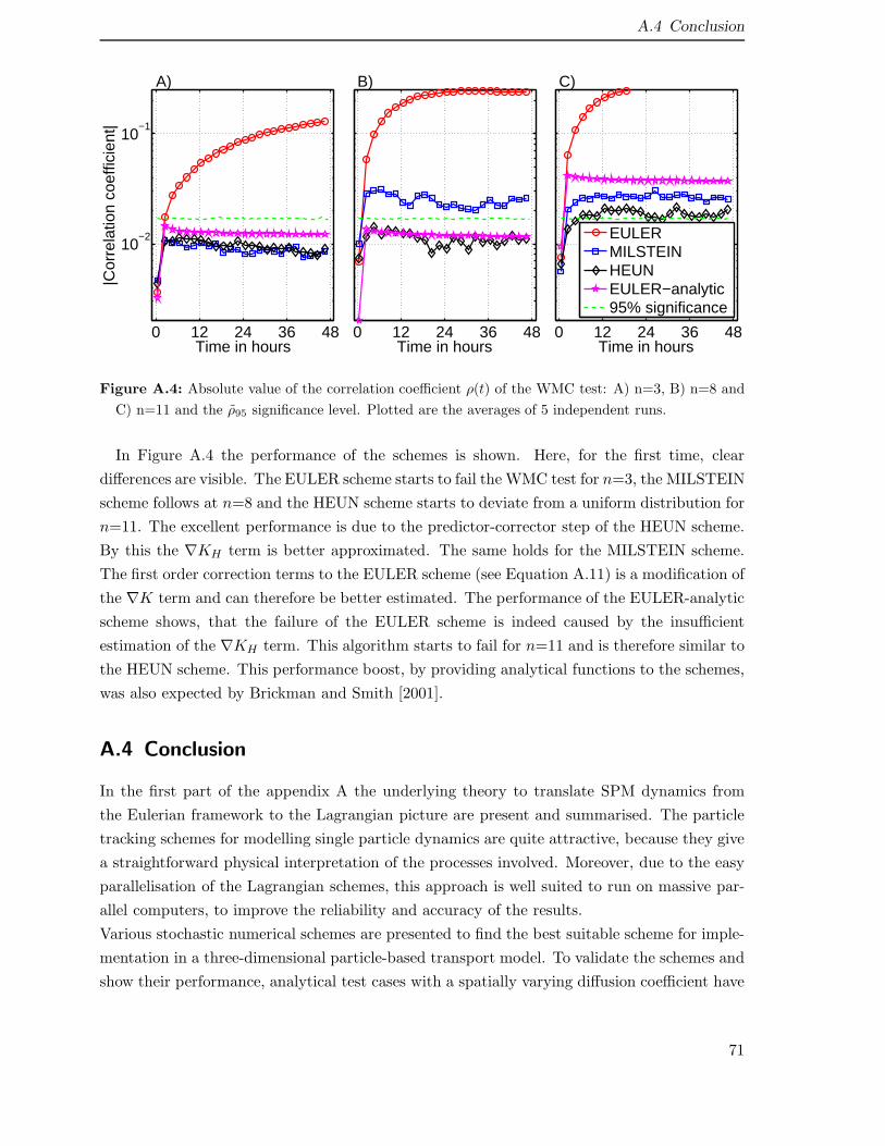
A.4 Conclusion
0 12 24 36 48
10−2
10−1
Time in hours
|Cor
rela
tion
coef
ficie
nt|
A)
0 12 24 36 48
Time in hours
B)
0 12 24 36 48
Time in hours
C)
EULERMILSTEINHEUNEULER−analytic95% significance .
Figure A.4: Absolute value of the correlation coefficient ρ(t) of the WMC test: A) n=3, B) n=8 and
C) n=11 and the ρ95 significance level. Plotted are the averages of 5 independent runs.
In Figure A.4 the performance of the schemes is shown. Here, for the first time, clear
differences are visible. The EULER scheme starts to fail the WMC test for n=3, the MILSTEIN
scheme follows at n=8 and the HEUN scheme starts to deviate from a uniform distribution for
n=11. The excellent performance is due to the predictor-corrector step of the HEUN scheme.
By this the ∇KH term is better approximated. The same holds for the MILSTEIN scheme.
The first order correction terms to the EULER scheme (see Equation A.11) is a modification of
the ∇K term and can therefore be better estimated. The performance of the EULER-analytic
scheme shows, that the failure of the EULER scheme is indeed caused by the insufficient
estimation of the ∇KH term. This algorithm starts to fail for n=11 and is therefore similar to
the HEUN scheme. This performance boost, by providing analytical functions to the schemes,
was also expected by Brickman and Smith [2001].
A.4 Conclusion
In the first part of the appendix A the underlying theory to translate SPM dynamics from
the Eulerian framework to the Lagrangian picture are present and summarised. The particle
tracking schemes for modelling single particle dynamics are quite attractive, because they give
a straightforward physical interpretation of the processes involved. Moreover, due to the easy
parallelisation of the Lagrangian schemes, this approach is well suited to run on massive par-
allel computers, to improve the reliability and accuracy of the results.
Various stochastic numerical schemes are presented to find the best suitable scheme for imple-
mentation in a three-dimensional particle-based transport model. To validate the schemes and
show their performance, analytical test cases with a spatially varying diffusion coefficient have
71

A Particle tracking schemes
been investigated. All of the three idealised test cases were performed with different numerical
schemes: EULER, MILSTEIN and HEUN. Even though the MILSTEIN scheme only requires
a minor additional effort compared with the EULER scheme, the changes in terms of higher
accuracy and faster convergence are rewarding. A two-step scheme like the HEUN scheme
leads to a further improvement of the results. The set of experiments that was carried out
indicates that any improvement over the EULER scheme is welcome. Even though this is not
trivial, and some care needs to be taken in the choice and application of the scheme, such
a scheme does not necessarily need to be complicated or expensive. As advanced as higher
order Lagrangian particle transport models for dispersion in turbulent flow sometimes are,
it is surprising to see how many of these models still use the EULER scheme, while minor
adaptations may greatly improve the accuracy of the model. The analysis also showed, that
especially the term ∇ · K in Equation (A.3) needs special care. The effort, to improve the
estimates of the gradient, results in performance gains. Further the validation of the three
tracking schemes revealed that although they have by definition the same order of convergence,
differences showed up.
72

Bibliography
Arnold L (1974) Stochastic differential equations, Wiley, New York
AVISO - Archiving, Validation and Interpretation of Satellite Oceanographic data,
[http://www.aviso.oceanobs.com]
Banas NS and Hickey BM (2005) Mapping exchange and residence time in a model of Willapa
Bay, Washington, a branching, macrotidal estuary. Journal of Geophysical Research 110, C11011,
DOI:10.1029/2005JC002950
Beckman A, Haidvogel D (1993) Numerical simulation of flow around a tall isolated seamount. Journal
of Physical Oceanography 23:1736-1753
Beer T, Borgas M, Bouma W, Fraser P, Holper P, Torok S (2006) Atmosphere. Theme commentary
prepared for the 2006 Australia State of the Environment Committee, Department of Environment
and Heritage, Canberra
Berkelmans R, Oliver JK (1999) Large-scale bleaching of corals on the Great Barrier Reef. Coral Reefs
18:55-60
Bignami F, Marullo S, Santoleri R, Schiano ME (1995) Longwave radiation budget in the Mediterranean
Sea. Journal of Geophysical Research 100:2501-2514
Bowers DG, Lennon GW (1987) Observations of stratified flow over a bottom gradient in a coastal sea.
Continental Shelf Research 7:1105-1121
Bureau of Meteorology, Australia, BOM, Australian Government, [http://www.bom.gov.au/]
Boyd R, Ruming K, Davies S, Payenberg T, Lang S (2004) Fraser Island and Hervey Bay e a classic
modern sedimentary environment, In: Boult, P.J., Johns, D.R., Lang, S.C. (Eds.) Eastern Australian
Basins Symposium II. Petroleum Exploration Society of Australia pp. 511-521 (special publication)
Burchard H, Petersen O, Rippeth TP (1998) Comparing the performance of the k-ǫ and the Mellor-
Yamada two-equation turbulence models. Journal of Geophysical Research 103:10543-10554
Burchard H, Lass U, Mohrholz V, Umlauf L, Sellschopp J, Fiekas V, Bolding K, Arneborg L (2005)
Dynamics of medium-intensity dense water plumes in the Arkona Basin, Western Baltic Sea. Ocean
Dynamics 55:391-402
Brickman D, Smith PC (2001) Lagrangian stochastic modeling in coastal oceanography. Journal of
Atmosphere and Ocean Technology 19:83-99
73

Bibliography
Brink KH, Shearman RK (2006) Bottom boundary layer flow and salt injection from the continental
shelf to slope. Geophysical Research Letter 33:L13608
Cai W, Shi G, Cowan T, Bi D, Ribbe J (2005) The response of the southern annual mode, the East
Australian Current, and the southern mid-latitude ocean circulation to global warming. Geophysical
Research Letter 32:L23706
Campbell SJ, McKenzie LJ (2004) Flood related loss and recovery of intertidal seagrass meadows in
southern Queensland, Australia. Estuarine, Coastal and Shelf Science 60:477-490
Cencini M, Bec J, Biferale L, Boffetta G, Celani A, Lanotte AS, Musacchio S, Toschi F (2006) Dynamics
and statistics of heavy particles in turbulent flows. Journal of Turbulence 7:36-52
Chaloupka M, Osmond M, Kaufman G (1999) Estimating seasonal abundance trends and survival
probabilities of humpback whales in Hervey Bay (east coast Australia). Marine Ecology Progress
Series 184:291-301
Charles WM, van den Berg E, Lin HX, Heemink AW, Verlaan M (2008) Parallel and distributed
simulation of sediment dynamics in shallow water using particle decomposition approach. Journal of
Parallel and Distributed Computing 68:717-728
Chung TJ (2002) Computational Fluid Dynamics, Cambridge University Press, Cambridge
Cohen JE, Small C, Mellinger A, Gallup J, Sachs J, Vitousek PM, Mooney HA (1997) Estimates of
coastal populations. Science 278:1211-1212
deCastro M, Gomez-Gesteira M, Alvarez I, Prego R (2004) Negative estuarine circulation in the Ria of
Pontevedra (NW Spain). Estuarine, Coastal and Shelf Science 60:301-312
Deleersnijder E, Beckers JM, Delhez EJM (2006a) The residence time of settling in the surface mixed
layer. Environmental Fluid Mechanics 6:25-42
Deleersnijder E, Beckers JM, Delhez EJM (2006b) On the behaviour of the residence time at bottom
of the mixed layer. Environmental Fluid Mechanics 6:541-547
Fairall CW, Bradley EF, Rogers DP, Edson JB, Young GS (1996), Bulk parametrisation of air-sea fluxes
for tropical ocean-global atmosphere Coupled-Ocean Atmosphere Response Experiment. Journal of
Geophysical Research 101:3747-3764
Fairall CW, Bradley EF, Hare JE, Grachev AA , Edson JB (2003) Bulk Parameterization of Air-Sea
Fluxes: Updates and Verification for the COARE Algorithm. Journal of Climate 16:571-591
Fer I, Adlandsvik B (2008) Descent and mixing of the overow plume from Storfjord in Svalbard: an
idealized numerical model study. Ocean Science 4:115-132
Flather RA (1976) A tidal model of the northwest European continental shelf. Memories de la Societe
Royale des Sciences de Liege 10:141-164
GLOSS - Global Sea Level Observing System, [http://www.gloss-sealevel.org/]
74

Bibliography
Glynn PW (2006) Coral reef bleaching: facts, hypotheses and implications. Global Change Biology
2(6):495-509
Grawe U, Wolff J-O, Ribbe J (2009) Mixing, Hypersalinity and Gradients in Hervey Bay, Australia.
Ocean Dynamics DOI: 10.1007/s10236-009-0195-4
Grawe U, Wolff J-O, Ribbe J (2009) Impact of climate variability on an east Australian bay. Estuarine,
Coastal and Shelf Science submitted to Estuarine, Coastal and Shelf Science
Grawe U, Wolff J-O (2009) Suspended particulate matter dynamics in a particle framework. Environ-
mental Fluid Mechanics DOI: 10.1007/s10652-009-9141-8
Growns I, James M (2005) Relationships between river flows and recreational catches of Australian
bass. Journal of Fish Biology 66:404-414
Guyondet T, Koutitonsky VG, Roy S (2005) Effects of water renewal estimates on the oyster aquaculture
potential of an inshore area. Journal of Marine Systems 58:35-51
Haney RL (1991) On the Pressure Gradient Force over Steep Topography in Sigma Coordinate Ocean
Models. Journal Physical Oceanography 21:610-619
Hoegh-Guldberg O (2009) Climate change and coral reefs: Trojan horse or false prophecy? Coral Reefs
DOI 10.1007/s00338-009-0508-6
Hunter JR, Craig PD, Phillips HE (1993) On the use of random walk models with spatially variable
diffusivity. Journal of Computational Physics 106:366-376
Intergovernmental panel on climate change, IPCC, ”Climate Change 2007”, the Fourth IPCC Assess-
ment Report, [http://www.ipcc.ch/ipccreports/]
Ivanov VV, Shapiro GI, Huthnance JM, Aleynik DL, Golovin PN (2004) Cascades of dense water
around the world ocean. Progess in Oceanography 60:47-98
Josey SA, Pascal RW, Taylor PK, Yelland MJ (2003) A New Formula For Determining the Atmospheric
Longwave Flux at the Ocean Surface at Mid-High Latitudes. Journal of Geophysical Research 108(C4)
Kennish MJ, Livingston RJ, Raffaelli D, Reise K (2008) Environmental future of estuaries. In: N.V.C.
Polunin (Ed.), Aquatic Ecosystems: Trends and Global Prospects, Cambridge University Press,
Cambridge, pp. 188-208
Kloeden PE, Platen E (1992) Numerical solutions of stochastic differential equations, Springer, Berlin
Heidelberg New York
Knauss JA (1978) Introduction to Physical Oceanography. Prentice Hall, Englewood Cliff, N.J., 338 pp
Krestenitis YN, Kombiadou KD, Savvidis YG (2007) Modelling the cohesive sediment transport in the
marine environment: the case of Thermaikos Gulf. Ocean Science 3:91-104
Labonne M, Morize E, Scolan P, Lae R, Dabas E, Bohn M (2009) Impact of salinity on early life
history traits of three estuarine fish species in Senegal. Estuarine, Coastal and Shelf Science DOI:
10.1016/j.ecss.2009.03.005
75

Bibliography
Largier JL, Hollibaugh JT, Smith SV (1997) Seasonally hypersaline estuaries in Mediterranean-climate
regions. Estuarine, Coastal and Shelf Science 45:789-797
Lavin MR, Godinez VM, Alvarez LG (1998) Inverse-estuarine Features of the Upper Gulf of California.
Estuarine, Coastal and Shelf Science 47:769-795
Lennon GW, Bowers DG, Nunes RA, Scott BD, Ali M, Boyle J, Wenju C, Herzfeld M, Johansson G,
Nield S, Petrusevics P, Stephanson P, Suskin AA, Wijffels SEA (1987) Gravity currents and the
release of salt from an inverse estuary. Nature 327:695-697
Lester RE, Fairweather PG (2009) Modelling future conditions in the degraded semi-arid estuary
of Australia’s largest river using ecosystem states. Estuarine, Coastal and Shelf Science, DOI:
10.1016/j.ecss.2009.04.018
Loder JW, Greenberg DA (1986) Predicted positions of tidal fronts in the Gulf of Maine region. Journal
of Geophysical Research 6:394-414
Luyten P J, Jones JE, Proctor R, Tabor A, Tett P, Wild-Allen K (1999) COHERENS - A coupled
hydrodynamical-ecological model for regional and shelf seas: user documentation, MUMM Rep.,
Management Unit of the Mathematical Models of the North Sea
Lyard F, Lefevre F, Letellier T, Francis O (2006) Modelling the global ocean tides: modern insights
from FES2004. Ocean Dynamics 56:394-415
Maier-Reimer E, Sundermann J (1982) On tracer methods in computational hydrodynamics, Engineer-
ing applications of computational hydraulics, Pitman Advanced Publ. Program, Boston, 198-217
Martinho AS, Batteen ML (2006) On reducing the slope parameter in terrain-following numerical ocean
models. Ocean Modelling 13:166-175
Masoner JR, Stannard DI, Christenson SC (2008) Differences in evaporation between a floating pan
and class A pan on land. Journal of the American water resources association 44:3-17
Matsumoto M, Nishimura T (1998) Mersenne Twister: A 623-Dimensionally Equidistributed Uni-
form Pseudo-Random Number Generator. ACM Transactions on Modeling and Computer Simulation
8(1):19-28
Mellor GL, Yamada T (1982) Development of a turbulence closure model for geophysical fluid problems.
Review of Geophysical Space Physics 20:851-875
Meynecke JO, Lee SY, Duke NC, Warnken J, (2006) Effect of rainfall as a component of climate
change on estuarine fish production in Queensland, Australia. Estuarine, Coastal and Shelf Science
69:491-504
Mikhailova VN, Isupovab MV (2008) Hypersalinization of River Estuaries in West Africa. Water Re-
sources, 35(4):367-385
Middleton JH, Coutis P, Griffin DA, Macks A, McTaggart A, Merrield MA, Nippard GJ (1994) Cir-
culation and Water Mass Characteristics of the Southern Great Barrier Reef. Australian Journal of
Marine Freshwater Research 45:1-18
76

Bibliography
Monin A, Obukhov A (1954) Basic turbulent mixing laws in the atmospheric surface layer. Trans
Geophys Inst Akad Nauk USSR 151:163-187
Murphy BF, Ribbe J (2004) Variability of southeast Queensland rainfall and its predictors. Journal of
Climatology 24(6):703-721
NOAA, National Weather Service, Center for Climate Prediction, [http://gcmd.nasa.gov/]
NODC - National Oceanographic Data Center, USA, National Environmental Satellite, Data and In-
formation Service, [http://www.nodc.noaa.gov]
Nof D (1983) The translation of isolated cold eddies on a sloping bottom. Deep Sea Research, Part A
30:171-182
North EW, Hood RR, Chao SY, Sanford LP (2006) Using a random displacement model to simulate
turbulent particle motion in a baroclinic frontal zone: A new implementation scheme and model
performance tests. Journal of Marine Systems 60:365-380
Nunes Vaz RA, Lennon GW, Bowers DG (1990) Physical behaviour of a large, negative or inverse
estuary. Continetal Shelf Research 10:277-304
Officer CB (1976) Physical Oceanography of Estuaries (and Associated Coastal Waters). Wiley, New
York, 465 pp.
Oke PR, Middleton JH (1999) Topographically Induced Upwelling off Eastern Australia. Journal of
Physical Oceanography 30:512-531
Pawlowicz R, Beardsley B, Lentz S (2002) Classical tidal harmonic analysis including error estimates
in MATLAB using T TIDE. Computational Geoscience 28:929-937
Pederson FB (1980) A monograph on turbulent entrainment and friction in two-layer stratified flow.
Series paper 25, Institute of Hydrodynamics and Hydraulic Engineering, Technical University of
Denmark
Prandle DA (1984) A modeling study of the mixing of 137Cs in the sea of the European continental
shelf. Philosophical Transaction of the Royal Society of London 310:407-436
Preen, AR, Lee Long WJ, Coles RG, (1995) Flood and cyclone related loss, and partial recovery, of
more the 1000 km2 of seagrasses in Hervey Bay, Queensland, Australia. Aquatic Botany 52:3-17
Press WH, Flannery BP, Teukolsky SA, Vetterling WT (1986) Numerical Recipes: The Art of Scientific
Computing, Cambridge University Press
Pritchard DW (1960) Salt balance and exchange rate for Chincoteague Bay. Science 1:48-57
Rayment GE, Neil D, (1997) Sources of material in river discharge. The Great Barrier Reef: Science,
Use and Management, James Cook University, Townsville 1:42-59
Ribbe J (2006) A study into the export of saline water from Hervey Bay, Australia. Estuarine, Coastal
and Shelf Science 66:550-558
77

Bibliography
Ribbe J, Wolff J-O, Staneva J, Grawe U (2008) Assessing Water Renewal Time Scales for Marine
Environments from Three-Dimensional Modelling: A Case Study for Hervey Bay, Australia. Envi-
ronmental Modelling Software 23:1217-1228
Ribbe J (2008) Monitoring and Assessing Salinity and Temperature Variations in Hervey
Bay. Final Report prepared for the Burnett Mary Regional Group, Bundaberg, Australia
[http://www.usq.edu.au/users/ribbe/]
Ridgway KR, Godfrey JS (1997) Seasonal cycle of the East Australian Current. Journal Geophysical
Research 102:22921-22936
Roe PL (1985) Some contributions to the modelling of discontinuous flows. In: Proceedings of 1983
AMS-SIAM summer seminar on large scale computing in fluid mechanics, Philadelphia. Lectures in
Applied Mathematics 22:163-193
Røed LP, Albertsen J (2007) The impact of freshwater discharge on the ocean circulation on the
Skagerrak/northern North Sea area Part I: model validation. Ocean Dynamics 57:296-285
Rolinski S, Umgiesser G (2005) Modelling short-term dynamics of suspended particulate matter in
Venice Lagoon. Estuarine, Coastal and Shelf Science 63:561-576
Roy PS, Williams RJ, Jones AR, Yassini I, Gibbs PJ, Coastes B, West RJ, Scanes PR, Hudson JP,
Nichols S (2001) Structure and function of south east Australian estuaries. Estuarine, Coastal and
Shelf Science 53:351-384
Saunders P, Coward AC, de Cuevas BA (1999) Circulation of the Pacific Ocean seen in a global ocean
model: Ocean Circulation and Climate Advanced Modelling project (OCCAM). Journal of Geophys-
ical Research 104:18281-18299
Schaffelke B, (2002) A review of water quality issues influencing the habitat quality in dugong protection
areas. Great Barrier Reef Marine Park Authority, Research Publication 66:78
Seidel DJ, Fu Q, Randel WJ, Reichler TJ (2008) Widening of the tropical belt in a changing climate.
Nature 104:18281-18299
Shapiro GI, Hill AE (1997) Dynamics of dense water cascades at the shelf edge. Journal of Physical
Oceanography 27:2381-2394
Shapiro GI, Huthnance JM, Ivanov VV (2003) Dense water cascading off the continental shelf. Journal
of Geophysical Research 108(C12):33-90
Shi G, Cai W, Cowan T, Ribbe J, Rotstayn L, Dix M (2008a) Variability and trend of the northwest
Western Australia Rainfall: observations and coupled climate modelling. Journal of Climate 21:2938-
2959
Shi G, Ribbe J, Cai W, Cowan T (2008b) Interpretation of Australian summer and winter rainfall
projections. Geophysical Research Letter 35:L02702
de Silva Samarasinghe JR (1998) Revisiting Upper Gulf St Vincent in South Australia: the Salt Balance
and its Implications. Estuarine, Coastal and Shelf Science 46:51-63
78

Bibliography
Simpson JH, Hunter JR (1974) Fronts in the Irish Sea. Nature 250:404-406
Simpson JH, Brown J, Matthews J, Allen G (1990) Tidal straining, density currents and stirring in the
control of estuarine stratification. Estuaries and Coasts 13:123-132
Simpson, JH, Sharples (1994) Does the earth’s rotation influence the location of the shelf sea fronts?
Journal of Geophysical Research 9(C2):3315-3319
Smagorinsky J (1963) General circulation experiments with the primitive equations I. The basic ex-
periment. Monthly Weather Review 91:99-165
Stijnen JW, Heemink AW, Lin HX (2006) An efficient 3D particle transport model for use in stratified
flows. International Journal of Numerical Methods in Fluids 51:331-350
Spivakovskaya D, Heemink AW, Deleersnijder E (2007) Lagrangian modelling of multi-dimensional
advection-diffusion with space-varying diffusivities: theory and idealised test cases. Ocean Dynamics
57:189-203
Staunton-Smith J, Robins JB, Mayer DG, Sellin MJ, Halliday IA, (2004) Does the quantity and timing
of fresh water flowing into a dry tropical estuary affect year-class strength of barramundi (Lates
calcarifer)? Marine and Freshwater Research 55:787-797
Swanson JC, Mendelsohn D (1996) BAYMAP, a simplified embayment flushing and transport model.
In: Spaulding, M., Cheng, R. (Eds.), Proceedings of the 4th International Conference on Estuarine
and Coastal Modeling. CA, San Diego
Tanny J, Cohen S, Assouline S, Lange F, Grava A, Berger D, Teltch B, Parlange MB (2008) Evaporation
from a small water reservoir: Direct measurements and estimates. Journal of Hydrology 351:218-229
Tomczak M (1985) The Bass Strait water cascade during winter 1981. Continental Shelf Research
4:255-278
Tomczak M, Godfrey S (2003) Regional Oceanography: an Introduction. 2nd edition. Daya Publishing
House Delhi, 390 pp
Ward TM, Staunton-Smith J, Hoyle S, Halliday IA (2003) Spawning patterns of four species of pre-
dominantly temperate pelagic fishes in the subtropical waters of southern Queensland. Estuarine,
Coastal Shelf Science 56:1125-1140
van de Kreeke J (1983) Residence time: application to small boat basins. ASCE Journal of Waterway,
Port, Coastal and Ocean Engineering 109:416-428
Vethamony P, Babu MT, Ramanamurty MV, Saran AK, Joseph A, Sudheesh K, Padgaonkar RS,
Jayakumar S (2007) Thermohaline structure of an inverse estuary - The Gulf of Kachchh: Measure-
ments and model simulations. Marine Pollution Bulletin 54:697-707
Visser AW (1997) Using random walk models to simulate the vertical distribution of particles in a
turbulent water column. Marine Ecology Progress Series 158:275-281
79

Bibliography
Visser AW (2008) Lagrangian modelling of plankton motion: From deceptively simple random walks
to Fokker-Planck and back again. Journal of Marine Systems 70:287-299
Warner JC, Sherwood CR, Arango HG, Signell RP (2005) Performance of four turbulence closure
models implemented using a generic length scale method. Ocean Modelling 8:81-113
Wolanski E (1986) An evaporation-driven salinity maximum zone in Australian tropical estuaries. Es-
tuarine, Coastal and Shelf Science 22:415-424
Zimmerman JTF (1988) Estuarine residence times. In: Kjerfve, B.(Ed.), Hydrodynamics of Estuaries
1, Estuarine Physics. CRC Press, Inc., Boca Raton, Florida, 76-84
80

Acknowledgements
At the end of this 3-year journey, leading to these final pages of my thesis, it is time to take
a bow and to acknowledge all the helpful people who pampered me with their kind support
along the way.
First, I am indebted to my supervisor Jorg-Olaf Wolff who invited me to work with him.
He was also ensuring fair funding for the years of my study. Further, I would also like to
express my gratitude for his friendly and permanent advice, guidance, the comfy working en-
vironment, the possibility to travel to Australia, to take part in summer schools and finally to
offer me the chance to discover parts of the ocean.
I would like to thank Joachim Ribbe for his help and to offer me the possibility to stay in Oz.
I am grateful to Emil Stanev for his kind support and to be finally my second supervisor.
I would also like to acknowledge the Wolfgang Schulenberg-Programm, the Universitats-
Gesellschaft Oldenburg (UGO), the Deutsche Forschungs Gesellschaft (DFG) and the Burnett
Mary Regional Group, Australia, for travel grants and financial support.
I really have to express my admiration and gratitude to the developers of COHERENS and
GETM for making their code available to the scientific community. I would also like to thank
the Mathworks Company for their excellent product MATLAB, the Linux community for
their fine OS and Intel for their breathtaking fast compilers.
A warm “thank you” goes to all my colleagues at the ICBM especially those mates (sorry, there
is no female version for mate) being members of the Theoretical Physics/Complex Systems
and Theoretical Physical Oceanography working group, the numerous coffee breaks, jokes and
laughing, discussions, cakes, music and motivation.
I would like to acknowledge Klemens for his selflessly care for the IT environment.
I further would like to thank Laird, Dave, Wes, Luc, and Spongebob for reminding me, that
the ocean is more than a discrete grid and that a wave is much more than a bump of water.
Further, I want to thank Oliver, who showed me how to shape a surfboard, ride a wave and
thus initiated an endless (summer) love story.
Special thanks goes to Pebbi and Carsten for offering me a second home in Oldenburg, Helmut
for being the most astonishing landlord I ever meet, Bastian and Antje for coffee, cake and
support and finally, Jens for help and motivation.
A special thanks goes to Maike, for the past, the present and the future.
Ultimately, I would like to mention my parents, but they know what I owing them.
CV
Ulf Grawe
born in Stralsund, July 12, 1974
Professional life
2005-2006 Researcher at ForWind - Wind Energy Research Insti-
tute/Oldenburg; modelling of the lower atmospheric boundary
layer and improvement of wind power predictions
1998-2002 4 years of travelling than a rolling Carpenter/Journeyman; work-
ing stays in Tunisia, Israel, Italy, Hungary, Switzerland, Austria,
France, Ireland, Germany, Estonia, Netherlands
Professional training
since October 2006 PhD student at the University of Oldenburg/ICBM - physical
oceanography (theory)
10/2005-08/2006 Student at the University of Oldenburg - Master of Science En-
gineering Physics (Thesis “Uncertainty estimation in wind power
predictions”), specialisation in turbulence, dynamical systems and
oceanography
10/2002-08/2005 Student at the University of Oldenburg - Bachelor of Engineering
Physics
1996-1998 Apprenticeship as carpenter, Carpentry Vifan GmbH Buschen-
hagen
Schooling
1981-1991 Herder-Realschule Stralsund
1991-1994 Technical Gymnasium Stralsund

Publikationsliste
Teile der vorliegenden Arbeit wurden bereits veroffentlicht oder eingereicht.
Grawe U, Wolff JO, Ribbe J (2009) Mixing, Hypersalinity and Gradients in Hervey Bay,
Australia. Ocean Dynamics DOI: 10.1007/s10236-009-0195-4 Grawe U, Wolff JO (2009) Suspended particulate matter dynamics in a particle frame-
work. Environmental Fluid Mechanics DOI: 10.1007/s10652-009-9141-8 Grawe U, Wolff JO, Ribbe J (2009) Impact of climate variability on an east Australian
bay. Estuarine, Coastal and Shelf Science eingereicht bei: Estuarine, Coastal and Shelf
Science
83

Selbstandigkeitserklarung
Hiermit erklare ich, dass ich die vorliegende Dissertation selbststandig verfasst und nur die
angegebenen Hilfsmittel verwendet habe. Teile der Dissertation wurden bereits in [Grawe et al. ,
2009a] und [Grawe and Wolff, 2009] veroffentlicht, bzw. sind zur Verweltlichung eingereicht
[Grawe et al. , 2009b]. Die Dissertation hat weder in Teilen noch in ihrer Gesamtheit einer an-
deren wissenschaftlichen Hochschule zur Begutachtung in einem Promotionsverfahren vorgele-
gen.
Oldenburg, September 16, 2009 Ulf Grawe