Heritability estimation in modern genetics and connections ...
19
Heritability estimation in modern genetics and connections to some new results for quadratic forms in statistics Lee H. Dicker Rutgers University and Amazon, NYC * Based on joint work with Ruijun Ma (Rutgers), Murat A. Erdogdu (Stanford/MSR), and Yakir Reshef (Harvard) Borchard Colloquium July 4, 2017 * Work conducted prior to joining Amazon
Transcript of Heritability estimation in modern genetics and connections ...

Heritability estimation in modern genetics andconnections to some new results for quadratic
forms in statistics
Lee H. DickerRutgers University and Amazon, NYC∗
Based on joint work withRuijun Ma (Rutgers), Murat A. Erdogdu (Stanford/MSR),
and Yakir Reshef (Harvard)
Borchard ColloquiumJuly 4, 2017
∗Work conducted prior to joining Amazon

Heritability in genetics
I Heritability is a fundamental concept in genetics. It represents the extentto which an exhibited trait in an individual is attributable to genetics.
I (Slightly) more technical formulation: The proportion of variation in aphenotype that can be explained by the genotype.
I Population-level estimates of heritability can be obtained from phenotypedata (e.g. human height or milk fat percentage in cows) and genotype data(e.g. pedigree information or GWAS data).
I Heritability estimation has a long history in statistics going back to R.A.Fisher.
I Currently, LMM-based methods are probably the most prevalant approachfor estimating heritability with GWAS data.
I LMM-based methods for heritability estimation are not new (Henderson, 1950,Ann. Math. Stat.).
I Modern LMM-based methods for GWAS data took off after (Yang et al., 2010,Nat. Genet.), which gave estimates of heritability for human height.
I Thousands of papers on LMM-based heritability for GWAS data since 2010.
1 / 15

Heritability in genetics
Hayes et al. (2010) PLoS Genet.
I Much of the recent work on LMM-based methods for heritability estimationis built on older research in to cattle breeding.
2 / 15

This talk
I Some new statistical perspectives on heritability estimation.I Main messages:
1. Standardize your predictors.2. There’s a big opportunity for statistics to make an impact in this
area with thoughtful modeling and technical expertise.
3 / 15
This talk
I Some new statistical perspectives on heritability estimation.I Main messages:
1. Standardize your predictors.
2. There’s a big opportunity for statistics to make an impact in thisarea with thoughtful modeling and technical expertise.
3 / 15

This talk
I Some new statistical perspectives on heritability estimation.I Main messages:
1. Standardize your predictors.2. There’s a big opportunity for statistics to make an impact in this
area with thoughtful modeling and technical expertise.
3 / 15

Genetic relatedness and heritabilityI Let y = (y1, . . . , yn)> ∈ Rn be a vector of centered real-valued outcomes,
where yi is the phenotype value for individual i in some population.
I Assume thaty = g + e (1)
can be decomposed into an additive genetic effect g ∼ MV(0, σ2gK) and an
uncorrelated noise vector e ∼ MV(0, σ2e I).
I K = (Kij) is the genetic relationship matrix (GRM) and Kij measures geneticsimilarity between individuals i and j; the GRM is standardized so that Kii = 1.
I The noise vector e may contain environmental noise, measurement error, andother non-additive genetic effects.
I Frequently, the data is transformed before reaching the representation (1), e.g.project out covariates or other fixed effects.
I The heritability coefficient is
h2 =σ2
g
σ2g + σ2
e.
I Since E(yy>) = σ2gK + σ2
e I, the heritability coefficient is the R2 forregressing yiyj on Kij , i.e. regressing phenotype similarity on geneticsimilarity.
4 / 15

Genetic relatedness and heritability
I To estimate h2, Henderson (1950) used least squares for regressing yiyj onKij .
I Maximum likelihood is also widely used: Let
`(s2g , s
2e ) =
12
log det(s2gK + s2
e I) +12
y>(s2gK + s2
e I)−1y
be the log-likelihood for (σ2g , σ
2e) under the assumption that g, e are
Gaussian; minimize ` to get the MLE for (σ2g , σ
2e) and h2.
I Henderson’s estimator and the MLE are both reasonable estimators for agiven GRM K — how should we choose K?
I Pre-GWAS: Pedigree/familial information determines K and describes howindividuals are related.
I Post-GWAS: Molecular genetic data gives fine-grained measure of geneticsimilarity.
5 / 15

Genetic relatedness and LMMs for GWAS data
I For GWAS data, each individual’s genetic data can be encoded in a vectorxi = (xi1, . . . , xim)> ∈ Rm, where xij represents the (frequently standardized)minor allele count for the j-th single nucelotide polymorphism (SNP).
I xij is tri-nary.I m can be in the 100K-1M’s; n may be in the 1-10K’s.
I The GRM is determined by a kernel function K with Kij = K(xi , xj). Thelinear kernel
K(xi , xj) =1m
x>i xj
is the most widely used in practice.
I With the linear kernel, the original model y = g + e can be rewritten as alinear random-effects model (LMM)
y = Xb + e,
where X = (x1, . . . , xn)>, b = (b1, . . . , bm)> ∈ Rm, andb1, . . . , bm ∼ MV(0, σ2
g/m) are iid.
6 / 15

LMMs for heritability estimation: Questions
y = Xb + e, (2)
I Variance components methods for estimating h2 under (2) have emergedas one of the most popular strategies for heritability estimation in GWAS.
I However, a number of challenges have emerged.I Causal SNPs and linkage disequilibrium. In most generative models for
linking GWAS data and outcomes, there is a fixed collection of causal SNPsC ⊆ [m] and b is assumed to be a sparse vector supported on C. If the SNPsxi are highly correlated — i.e. they are in linkage disequilibrium (LD) — theLMM approach can give badly biased estimates for h2 (Speed et al., 2012,Am. J. Hum. Genet.)
I Partitioning heritability. Sometimes it’s desirable to estimate the heritabilityattributable to a subset of SNPs, S ⊆ [m]. To date, there’s no consensus abouthow this should be done and existing solutions have significant drawbacks.
7 / 15

Causal SNPs and linkage disequilibrium
I Simulations show standard LMM estimators for h2 are biased when causalSNPs are located in regions with low (or high) LD.
I Settings:I n = 500, m = 1000.I σ2
e = 0.5.
I b =√
1m (z1, . . . , zm/2, 0, . . . , 0)> ∈ Rm with z1, . . . , zm/2 ∼ N(0, 1) iid. So
C = {1, . . . ,m/2}.
I xi ∼ N(0,Σ) with Σ =
(AR(0.2) 0
0 AR(0.8)
).
I Then σ2g = 0.5 and h2 = 0.5.
h2 h2
0.5 Mean: 0.43295% CI: (0.404,0.460)
Table: Summary of results based on simulating 50 independent datasets.
8 / 15

Partitioning heritabilityI One method for partitioning heritability is to assume a LMM with multiple
variance components (Finucane et al., 2015, Nat. Genet.):
y = XSbS + XSc bSc + e, (3)
where
bi ∼
MV
(0,
σ2S
|S|
), if i ∈ S,
MV(0,
σ2Sc
m−|S|
)if i < S
are all independent.
I The S-partitioned heritability is
h2S
=σ2S
σ2S
+ σ2Sc + σ2
e.
I h2S
can be estimated, for instance, using maximum for the model (3) under aGaussian random-effects assumption.
I However, estimating the total heritability h2 = (σ2S
+ σ2Sc )/(σ2
S+ σ2
Sc + σ2e)
under this model has the same issues noted in the previousslide/simulation.
9 / 15

LMMs for heritability estimation
I Challenges arise when the location of causal SNPs iscorrelated with LD structure.
I Solution:
Remove LD structure, i.e. whiten.
10 / 15
LMMs for heritability estimation
I Challenges arise when the location of causal SNPs iscorrelated with LD structure.
I Solution: Remove LD structure, i.e. whiten.
10 / 15
LMMs for heritability estimation: Mahalanobis kernel
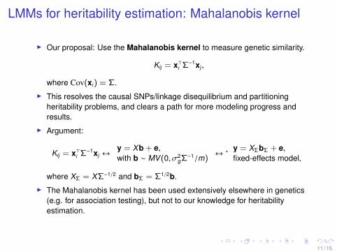
I Our proposal: Use the Mahalanobis kernel to measure genetic similarity.
Kij = x>i Σ−1xj ,
where Cov(xi) = Σ.
I This resolves the causal SNPs/linkage disequilibrium and partitioningheritability problems, and clears a path for more modeling progress andresults.
I Argument:
Kij = x>i Σ−1xj ↔y = Xb + e,with b ∼ MV(0, σ2
gΣ−1/m)↔ ∗ y = XΣbΣ + e,
fixed-effects model,
where XΣ = XΣ−1/2 and bΣ = Σ1/2b.
I The Mahalanobis kernel has been used extensively elsewhere in genetics(e.g. for association testing), but not to our knowledge for heritabilityestimation.
11 / 15

Revisiting Causal SNPs/LD and partitioning heritability
I To find the Mahalanobis-MLE h2Σ, replace X by XΣ−1/2 and then find the
MLE for h2 using the linear kernel, i.e. whiten/decorrelate/standardize thepredictors and compute the usual MLE.
h2 h2 h2Σ
0.5 Mean: 0.432 Mean: 0.49995% CI: (0.404,0.460) 95% CI: (0.473, 0.525)
I Let
Σ =
(ΣS,S ΣS,Sc
Σ>S,Sc ΣSc ,Sc
).
The partitioned heritability is defined via the decomposition
y = gS + gSc + e,
wheregS = XS(bS + Σ−1
S,SΣS,Sc bSc ),
gSc = (XSc − XSΣ−1S,SΣS,Sc )bSc .
I Under the LMM y = Xb + e with b ∼ MV(0, σ2gΣ−1/m), gS and gSc are
uncorrelated.
12 / 15

Why does this work?
I Model misspecification results for variance components estimationproblems (D & Erdogdu, 2016, 2017).
I Meta-result. Assume:
(i) y = Xb + e ∈ Rn
(ii) Cov(e) = σ2e .
(iii) b ∈ Rm is any (fixed or random) vector with ‖b‖2 � 1.
If xi ∼ N(0,Σ) are iid, then the variance component estimators for theMahalanobis kernel (σ2
g , σ2e) are nice:
(i) (σ2g , σ
2e)→ (σ2
g , σ2e), where σ2
g = lim ‖b‖2.(ii) (σ2
g , σ2e) are approximately normal.
I Implication: If genotypes are random, then the Mahalanobis kernel forestimating heritability works even with fixed genetic effects – and, inparticular, when the location of causal SNPs is associated with LDstructure.
13 / 15

Why does this work?I Proof idea: In the fixed-effects model with random genotypes, b inherits
randomness from X .
I Let θ = (σ2g , σ
2e) be the MLE and assume WLOG that xi ∼ N(0, I).
I Key point: Since X D= XU for any m ×m orthogonal matrix U,
θ(y,X)D= θ(y,X),
wherey = X b + e, b ∼ uniform{Sm−1(σ2
g)}.
I In other words, θ = θ(y,X) has the same distribution as θ(y,X), where thedata are drawn from a random-effects model.
I Since b is approximately Gaussian for large m, we can use tools forvariance components estimation in Gaussian random-effects models toapproximate the distribution of θ.
I Finite sample normal approximation results for quadratic forms.
I Other comments:I We can get closed form expressions for the asymptotic variance of θ using
results on the Marcenko-Pastur distribution.
14 / 15
Open questions
I Results for non-Gaussian xi .I SNP genotype data is always non-Gaussian, but simulations
suggest results may still hold.I Binary outcomes.
I Erdogdu, Bayati & D (2016).
I Applications to association testing problems.
15 / 15