HEMODYNAMIC DESIGN OPTIMIZATION OF A VENTRICULAR...
67
HEMODYNAMIC DESIGN OPTIMIZATION OF A VENTRICULAR CANNULA: EVALUATION AND IMPLEMENTATION OF OBJECTIVE FUNCTIONS by Samuel J. Hund Bachelors of Science in Engineering, University of Colorado, 1999 Masters of Science in Engineering, University of Colorado, 2001 Submitted to the Graduate Faculty of the School of Engineering in partial fulfillment of the requirements for the degree of Master of Science University of Pittsburgh 2006
Transcript of HEMODYNAMIC DESIGN OPTIMIZATION OF A VENTRICULAR...
HEMODYNAMIC DESIGN OPTIMIZATION OF A
VENTRICULAR CANNULA: EVALUATION AND IMPLEMENTATION OF OBJECTIVE
FUNCTIONS
by
Samuel J. Hund
Bachelors of Science in Engineering, University of Colorado, 1999
Masters of Science in Engineering, University of Colorado, 2001
Submitted to the Graduate Faculty of
the School of Engineering in partial fulfillment
of the requirements for the degree of
Master of Science
University of Pittsburgh
2006

UNIVERSITY OF PITTSBURGH
SCHOOL OF ENGINEERING
This thesis was presented
by
Samuel J. Hund
It was defended on
March 8th, 2006
and approved by
James F. Antaki, PhD, Department of Bioengineering and Department of Surgery
Harvey S. Borovetz, PhD, Department of Bioengineering and Department of Surgery
Anne M. Robertson, PhD, Department of Mechanical Engineering
Thesis Advisor: James F. Antaki, PhD, Bioengineering
ii

HEMODYNAMIC DESIGN OPTIMIZATION OF A VENTRICULAR CANNULA: EVALUATION AND IMPLEMENTATION OF OBJECTIVE FUNCTIONS
Samuel J. Hund, M.S.
University of Pittsburgh, 2006
Shape optimization has been used for decades to improve the aerodynamic performance of
automobiles and aircraft. The application of this technology to blood-wetted medical devices
have been limited, in part, due to the ambiguity of hemodynamic variables associated with
biocompatibility – specifically hemolysis, platelet activation, and thrombus formation. This
study undertook a systematic evaluation of several objective functions derived directly from the
flow field. We specifically focused on the optimization of a two-dimensional blood conduit
(cannula) by allowing free variation of the centerline and cross-sectional area. The flow was
simulated using computational fluid dynamics (CFD) at a nominal flow rate of 6 lpm and
boundary conditions consistent with an abdominally positioned left-ventricular-assist device
(LVAD). The objectives were evaluated both locally and globally. The results demonstrated
similarities between four of the functions: vorticity, viscous dissipation, principal shear stress,
and power-law (PL) blood damage models based on shear history. Of the functions analyzed,
those found to be most indicative of flow separation and clearance were flow deviation index and
the Peclet Number. The conclusions from these studies will be applied to ongoing development
of algorithms for optimizing the flow path of rotary blood pumps, cannula, and other blood
contacting devices.
iii

TABLE OF CONTENTS
PREFACE.................................................................................................................................VIII
1.0 INTRODUCTION AND BACKGROUND................................................................ 1
1.1 BLOOD DAMAGE.............................................................................................. 2
1.1.1 Composition and Rheology of Blood........................................................... 3
1.1.2 Hemolysis ....................................................................................................... 4
1.1.3 Platelet Activation......................................................................................... 5
1.1.4 Thrombosis and the Coagulation Cascade ................................................. 5
1.2 CURRENT METHODS FOR ANALYZING BLOOD DAMAGE................. 6
1.2.1 Indices for Estimating Hemolysis ................................................................ 7
1.2.2 Estimators of Recirculation and Stagnation............................................. 11
1.3 NUMERICAL METHODS FOR SOLVING PARTIAL DIFFERENTIAL
EQUATIONS ...................................................................................................................... 12
1.3.1 Finite Element Method............................................................................... 13
1.3.2 FEM for Fluid Flow.................................................................................... 13
1.4 SHAPE OPTIMIZATION ................................................................................ 14
1.4.1 General Topics in Optimization ................................................................ 14
1.4.1.1 Determining the Search Direction..................................................... 16
1.4.1.2 The Line Search .................................................................................. 18
1.4.1.3 Evaluating Optimality ........................................................................ 18
1.4.1.4 Handling Constraints in Optimization Problems ............................ 19
1.4.2 The Sequential Quadratic Programming Method for Optimization ..... 19
1.4.3 Multi-Objective Optimization.................................................................... 20
1.4.4 Shape Optimization in Fluid Dynamics .................................................... 21
2.0 METHODS ................................................................................................................. 23
iv

2.1 NUMERICAL METHODS............................................................................... 23
2.1.1 Computational Fluid Dynamics Using FEMLAB.................................... 23
2.1.2 Optimization Using the SQP Method........................................................ 24
2.2 ANALYZING OBJECTIVE FUNCTIONS .................................................... 24
2.2.1 Qualitative Analysis of Objective Functions ............................................ 24
2.2.2 Quantitative Analysis of Objective Functions.......................................... 27
2.3 OPTIMIZATION OF A 2-D CANNULA........................................................ 28
3.0 RESULTS OF OBJECTIVE FUNCTION ANALYSIS ......................................... 30
3.1 QUALITATIVE ANALYSIS OF OBJECTIVE FUNCTIONS .................... 30
3.2 QUALITATIVE ANALYSIS OF THE DESIGN SPACE ............................. 33
3.2.1 Evaluation of the Design Space.................................................................. 33
3.2.2 Summary of the Statistical Analysis.......................................................... 37
3.3 THE OPTIMIZED 2-D CANNULA ................................................................ 39
4.0 DISCUSSION AND CONLUSIONS ........................................................................ 43
4.1 QUALITATIVE ANALYSIS OF OBJECTIVE FUNCTIONS .................... 44
4.2 QUANTITATIVE ANALYSIS OF OBJECTIVE FUNCTIONS.................. 44
4.3 OPTIMIZATION OF A 2-D CANNULA........................................................ 48
5.0 FUTURE WORK ....................................................................................................... 50
BIBLIOGRAPHY....................................................................................................................... 52
v

LIST OF TABLES
Table 1: List of quantities that can estimate blood damage............................................................ 7
Table 2: Fitted values for various power-law models for blood damage. ...................................... 9
Table 3: The evaluation of each objective function in the selected designs. ................................ 33
Table 4: Correlation table for the design space analysis............................................................... 34
Table 5: Statistical evaluation of the objective functions. ............................................................ 37
Table 6: Objective function values in each of the optimum cannula............................................ 40
Table 7: First and second variations of selected objective functions............................................ 47
vi

LIST OF FIGURES
Figure 1: Flow through selected cannula plotted with pressure contours and velocity vectors. .. 25
Figure 2: Recirculation regions of bad cannula designs ............................................................... 26
Figure 3: Design space for the 2-D cannula.................................................................................. 28
Figure 4: Field plot of the several functions that represent shear induced hemolysis. ................. 31
Figure 5: Plot of function that relate to stagnation. The color is plotted logarithmically............. 32
Figure 6: Plot of the eigenvalues and their information percent................................................... 36
Figure 7: The optimal 2-D cannulas corresponding to various objective functions. .................... 40
Figure 8: The objective functions of the multi-objective optimized cannula. .............................. 41
Figure 9: Second set of multi-objective optimized (MOO) cannulae........................................... 42
vii

PREFACE
I would like to thank my thesis committee and all of those who helped advise me through the
years, include Robert Leben, Greg Burgreen, and Omar Ghattas. I would also like to thank the
Sangria Project and its members as well as the NSF Center for e-Design who were invaluable
collaborators over the past few years.
viii

1.0 INTRODUCTION AND BACKGROUND
The development of blood-wetted medical devices is very difficult and ill posed. The complex
nature of blood makes it difficult to completely simulate the biocompatibility of these devices.
Even when a suitable design is found, the results may not scale from one application to the next,
necessitating a redesign for each case. Despite these challenges, computer simulations and
numerical optimization provide practical and cost-effective methods for the design and
evaluation of these devices. The aerospace and automotive industries have used shape
optimization (SO) for several decades to improve their products. The biomedical industry has
seen an increase in the use computational fluid dynamics (CFD), but it is lagging behind other
major industries in its implementation; and has not adopted SO in any meaningfully way. One of
the challenges to implementing optimization into the biomedical industry is relating simulation
results to biocompatibility or biological performance. For example, Giersiepen (1) developed a
power-law model for blood trauma that was based on highly restricted conditions. Investigators
have attempted to apply it blindly to CFD analyses, but its validity under generalized conditions
has never been validated; hence its utility as a predictive tool is questioned(2, 3). Other
simulations of flow-related blood trauma, such as platelet deposition models presented by
Sorensen et al. (4, 5), have yet to be expanded to complex flow patterns similar to those found in
medical devices. The goal of this thesis is to carry out a systematic analysis of the most
commonly used macroscopic models (reduced order) for blood damage to predict microscopic
phenomena. Additional models were introduced to fill gaps that were perceived in describing the
relevant hemodynamic phenomena for biocompatibility.
The first section describes a detailed study leading to the selection of several key
functions representing blood damage, suitable for use as objective functions for blood-wetted
medical devices. The second section of this thesis involves applying these functions to a
benchmark problem, namely the ventricular cannula for a left ventricular assist device (LVAD),
1

such as the Streamliner VAD. This benchmark case was chosen for several reasons. Cannulae
have generally not been studied to the same extent as other hemodynamic problems – such as
end-to-side anastomosis. Of the few studies that have been performed on cannulae, most involve
material properties, while very little work has been done on the flow path(6-12). Secondly flow
through curved tubes, including cannula, is not trivial. The flow exhibits several interacting
phenomena such as separation and Dean Vortices. Finally, the flow profile exiting the cannula
can dramatically affect the performance of the VAD to which it is attached. In summary, the
study of flow in a cannula strikes a balance between simplicity and non-triviality: the problem is
simple enough to be tractable, yet complex enough so that the results are neither trivial nor
intuitive, but useful.
This thesis is organized in a logical fashion, beginning with an overview of the basics of
blood rheology and trauma. The following introductory sections describe some of the common
methods by which CFD is used to estimate blood damage, and introduces optimization in the
context of the finite element method (FEM). The Methods sections provides a more detailed
description of the specific methods and approaches employed n this study, including the blood
damage indicators chosen. The Results section describes the implementation of the objective
functions into the design of the cannula. The thesis concludes with a discussion of the results and
future work.
1.1 BLOOD DAMAGE
The design goal of any medical device is to maximize safety and efficacy. In this respect, blood
damage is one of the most important issues for blood-wetted devices. Blood damage refers to a
physiological and morphological change that occurs to any component of the blood, and can take
on several forms. The most traditional analysis of blood damage is hemolysis: the rupture of red
blood cells. Hemolysis can lead to hemoglobinemia or anemia. A second indicator of blood
damage is thrombosis, which is the leading cause of device failure and device related
complications (13). A third indicator is shear induced white blood cell and platelet activation, but
the underlying physics are similar to those behind hemolysis. It is important to have a basic
understanding of blood in order to understand how it is damaged, so a brief summary of blood is
2
provided in the following section, followed by a detailed discussion of how blood is damaged by
surface contact and flow conditions.
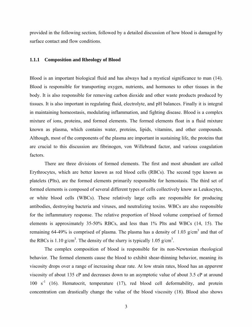
1.1.1 Composition and Rheology of Blood
Blood is an important biological fluid and has always had a mystical significance to man (14).
Blood is responsible for transporting oxygen, nutrients, and hormones to other tissues in the
body. It is also responsible for removing carbon dioxide and other waste products produced by
tissues. It is also important in regulating fluid, electrolyte, and pH balances. Finally it is integral
in maintaining homeostasis, modulating inflammation, and fighting disease. Blood is a complex
mixture of ions, proteins, and formed elements. The formed elements float in a fluid mixture
known as plasma, which contains water, proteins, lipids, vitamins, and other compounds.
Although, most of the components of the plasma are important in sustaining life, the proteins that
are crucial to this discussion are fibrinogen, von Willebrand factor, and various coagulation
factors.
There are three divisions of formed elements. The first and most abundant are called
Erythrocytes, which are better known as red blood cells (RBCs). The second type known as
platelets (Plts), are the formed elements primarily responsible for hemostasis. The third set of
formed elements is composed of several different types of cells collectively know as Leukocytes,
or white blood cells (WBCs). These relatively large cells are responsible for producing
antibodies, destroying bacteria and viruses, and neutralizing toxins. WBCs are also responsible
for the inflammatory response. The relative proportion of blood volume comprised of formed
elements is approximately 35-50% RBCs, and less than 1% Plts and WBCs (14, 15). The
remaining 64-49% is comprised of plasma. The plasma has a density of 1.03 g/cm3 and that of
the RBCs is 1.10 g/cm3. The density of the slurry is typically 1.05 g/cm3.
The complex composition of blood is responsible for its non-Newtonian rheological
behavior. The formed elements cause the blood to exhibit shear-thinning behavior, meaning its
viscosity drops over a range of increasing shear rate. At low strain rates, blood has an apparent
viscosity of about 135 cP and decreases down to an asymptotic value of about 3.5 cP at around
100 s-1 (16). Hematocrit, temperature (17), red blood cell deformability, and protein
concentration can drastically change the value of the blood viscosity (18). Blood also shows
3

some viscoelastic behavior (19), but the most significant signs of this phenomenon require the
blood to be motionless for upwards of 10 minutes (20). Sharp et al. and others show that
viscoelastic models of blood only show a 2% change in the peak velocity and a 3% change in
wall shear stress when viscoelastic models were employed for flow in a tube (21). This was
illustrated by a study of Mann et al. who showed that a solutions separan and xantham gum,
which exhibits viscoelastic and shear-thinning behavior, approximated the shear stress profiles of
blood in an experimental VAD better than a pure Newtonian fluid (22, 23).
1.1.2 Hemolysis
Hemolysis, or blood cell lysis, typically refers to the rupture of the membrane of the red blood
cell and liberation of its contents, primarily hemoglobin. Although research of mechanical
trauma to blood has been studied for decades, investigation into the microscopic mechanisms of
shear induced hemolysis is still in its infancy (24). It is known that red blood cells are resistant to
large compressive pressures up 2000 mmHg, but can easily be ruptured by exposure to small
shearing forces around 200 mmHg (25-28). There is also a complex shear-exposure relationship,
where a red blood cell can survive large stresses (1.5-3000 mmHg) for short periods of time (1,
28). Pressure gradients and fluctuations have been shown to cause hemolysis (29-32). Kuchar
and Sutera predicted that flow features that cause hemolysis are turbulence, geometries that
produce high-shear stresses, sharp corners, stagnation regions, and flow separation, but Sutera
showed that turbulence only increased hemolysis near walls (33, 34).
If a large number of RBCs are destroyed over a short period of time, a lethal level
(approximately 160 mg/dL) of hemoglobin can develop in the blood stream causing renal failure
and possibly death (35-37). Several steps are required to remove hemoglobin from the free
stream (14). First it is picked up by Macrophages, then its iron is stripped and the protein
digested. The iron is then bound to a protein called transferrin and is released back into the blood
stream where it can be used just like dietary iron (14).
Even if hemolysis is not high enough to cause hemoglobinemia, it may still pose a danger
because of anemia. Although not a fatal condition anemia caused by long term blood cell
destruction can results in weakness, slower healing, lower exercise tolerance, and a lower quality
4

of life. Hemolysis is also an indicator of a more dangerous, but less easily detected phenomena
of platelet activation, describe below.
1.1.3 Platelet Activation
Platelets activation can be accomplished through several mechanisms. The platelet acts as the
first line of defense in blood clotting by activating when contacting a foreign surface, which
forms a “plug” when collagen is exposed by damaged tissue. Platelets can also activate when
coming into contact with certain chemicals, known as agonists, such as adenosine-diphosphate
(ADP), thrombin, and Thromboxane A2 (TxA2) (38). Surface and chemical activation of
platelets is irreversible and results in the release of agonists, an inversion of the membrane,
receptor activation, and other conformal changes. Activated platelets that remain in the blood
stream are usually cleared from the circulation in the spleen. Shear stress can also activate
platelets directly, but this can be either reversible or irreversible (39). Reversible activation only
results in changes in fibrinogen receptor that increases the likelihood of aggregates forming.
Activated platelets are also more likely to stick to the surface and other activated platelets. The
deleterious consequences of platelet activation in prosthetic blood-wetted devices can be quite
catastrophic.
1.1.4 Thrombosis and the Coagulation Cascade
Blood loss can be life threatening, so all of the components necessary to stop bleeding are
actively floating through the body in an inert state. If a blood vessel is ruptured exposing the
underlying collagen, the body can almost instantaneously start the process to clot through platelet
adhesion and the coagulation cascade. Unfortunately, artificial surfaces can activate the same
mechanisms, which could lead to device failure or injury to the patients.
Virchow’s triad elegantly ties thrombosis to the contacting surface, the blood properties,
and the fluid flow. The surface effects and methods of mitigating them are beyond the scope of
this work, so only the basic principals will be discussed here. Coagulation involves the activation
of platelets and a complex cascade of protein reaction that results in a solid thrombus. Major
5
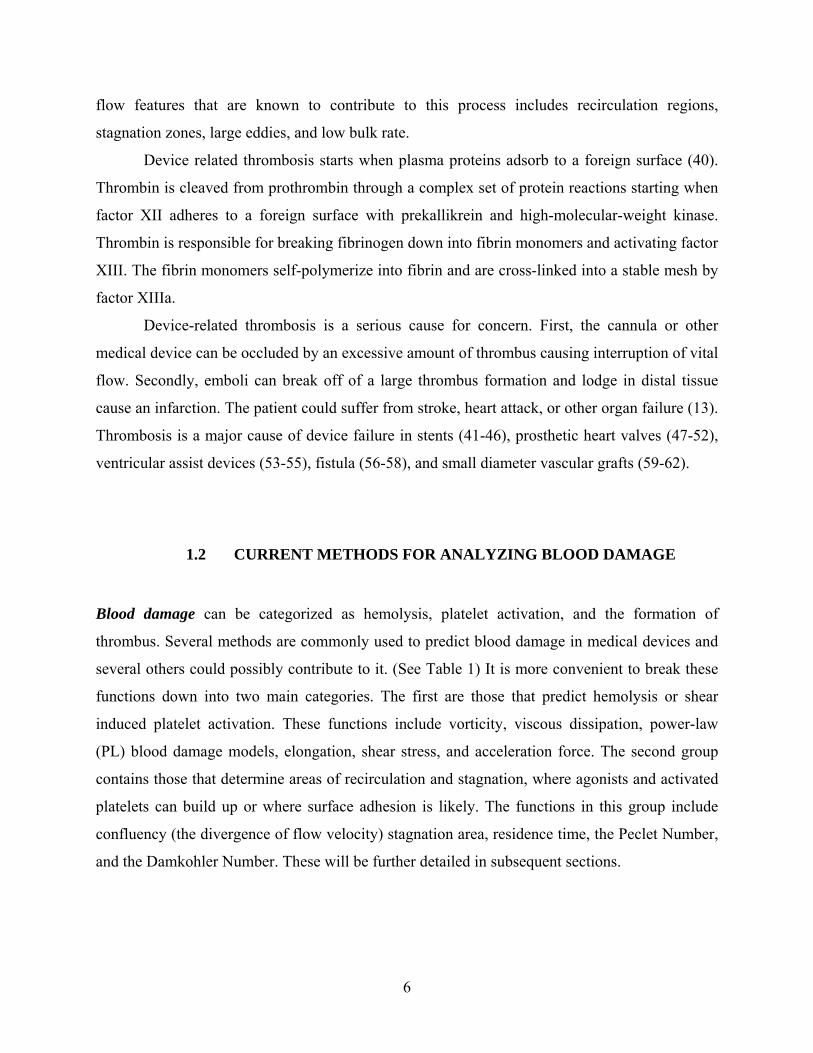
flow features that are known to contribute to this process includes recirculation regions,
stagnation zones, large eddies, and low bulk rate.
Device related thrombosis starts when plasma proteins adsorb to a foreign surface (40).
Thrombin is cleaved from prothrombin through a complex set of protein reactions starting when
factor XII adheres to a foreign surface with prekallikrein and high-molecular-weight kinase.
Thrombin is responsible for breaking fibrinogen down into fibrin monomers and activating factor
XIII. The fibrin monomers self-polymerize into fibrin and are cross-linked into a stable mesh by
factor XIIIa.
Device-related thrombosis is a serious cause for concern. First, the cannula or other
medical device can be occluded by an excessive amount of thrombus causing interruption of vital
flow. Secondly, emboli can break off of a large thrombus formation and lodge in distal tissue
cause an infarction. The patient could suffer from stroke, heart attack, or other organ failure (13).
Thrombosis is a major cause of device failure in stents (41-46), prosthetic heart valves (47-52),
ventricular assist devices (53-55), fistula (56-58), and small diameter vascular grafts (59-62).
1.2 CURRENT METHODS FOR ANALYZING BLOOD DAMAGE
Blood damage can be categorized as hemolysis, platelet activation, and the formation of
thrombus. Several methods are commonly used to predict blood damage in medical devices and
several others could possibly contribute to it. (See Table 1) It is more convenient to break these
functions down into two main categories. The first are those that predict hemolysis or shear
induced platelet activation. These functions include vorticity, viscous dissipation, power-law
(PL) blood damage models, elongation, shear stress, and acceleration force. The second group
contains those that determine areas of recirculation and stagnation, where agonists and activated
platelets can build up or where surface adhesion is likely. The functions in this group include
confluency (the divergence of flow velocity) stagnation area, residence time, the Peclet Number,
and the Damkohler Number. These will be further detailed in subsequent sections.
6
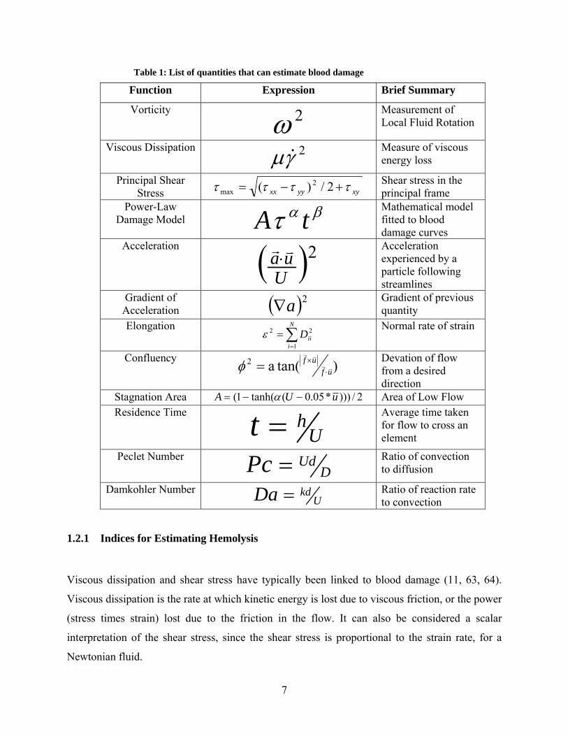
Table 1: List of quantities that can estimate blood damage
Function Expression Brief Summary
Vorticity 2ω
Measurement of Local Fluid Rotation
Viscous Dissipation 2γμ & Measure of viscous energy loss
Principal Shear Stress xyyyxx ττττ +−= 2/)( 2
max Shear stress in the principal frame
Power-Law Damage Model βατ tA
Mathematical model fitted to blood damage curves
Acceleration ( )2Uua vr⋅
Acceleration experienced by a particle following streamlines
Gradient of Acceleration ( )2a∇
Gradient of previous quantity
Elongation ∑=
=N
iiiD
1
22ε Normal rate of strain
Confluency )tan(a2uf
ufvv
vv
⋅×=φ
Devation of flow from a desired direction
Stagnation Area 2/)))*05.0(tanh(1( uUA −−= α Area of Low Flow Residence Time
Uht =
Average time taken for flow to cross an element
Peclet Number D
UdPc = Ratio of convection to diffusion
Damkohler Number U
kdDa = Ratio of reaction rate to convection
1.2.1 Indices for Estimating Hemolysis
Viscous dissipation and shear stress have typically been linked to blood damage (11, 63, 64).
Viscous dissipation is the rate at which kinetic energy is lost due to viscous friction, or the power
(stress times strain) lost due to the friction in the flow. It can also be considered a scalar
interpretation of the shear stress, since the shear stress is proportional to the strain rate, for a
Newtonian fluid.
7
Most research into hemolysis directly relates it to shear stress (11, 25-28, 63-65). Shear
stress is a difficult parameter to examine because it is a tensor quantity. The most common
methods for analyzing stress is to calculate the norm of the tensor. The simplest form for two and
three-dimensional flow is the product of viscosity and shear rate: γμ & , or alternatively the
maximum principal stress: maxτ . Only the maximum principal shear stress will be analyzed, since
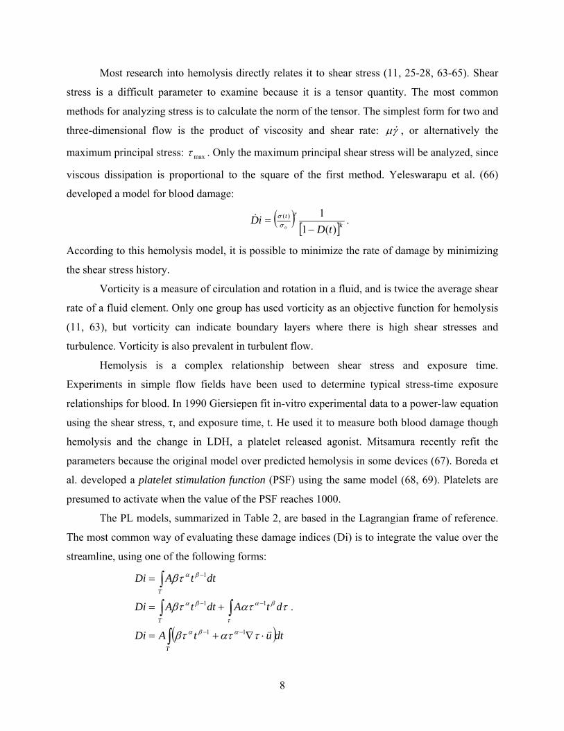
viscous dissipation is proportional to the square of the first method. Yeleswarapu et al. (66)
developed a model for blood damage:
( )[ ]k
rt
tDiD
o )(11)(
−= σ
σ& .
According to this hemolysis model, it is possible to minimize the rate of damage by minimizing
the shear stress history.
Vorticity is a measure of circulation and rotation in a fluid, and is twice the average shear
rate of a fluid element. Only one group has used vorticity as an objective function for hemolysis
(11, 63), but vorticity can indicate boundary layers where there is high shear stresses and
turbulence. Vorticity is also prevalent in turbulent flow.
Hemolysis is a complex relationship between shear stress and exposure time.
Experiments in simple flow fields have been used to determine typical stress-time exposure
relationships for blood. In 1990 Giersiepen fit in-vitro experimental data to a power-law equation
using the shear stress, τ, and exposure time, t. He used it to measure both blood damage though
hemolysis and the change in LDH, a platelet released agonist. Mitsamura recently refit the
parameters because the original model over predicted hemolysis in some devices (67). Boreda et
al. developed a platelet stimulation function (PSF) using the same model (68, 69). Platelets are
presumed to activate when the value of the PSF reaches 1000.
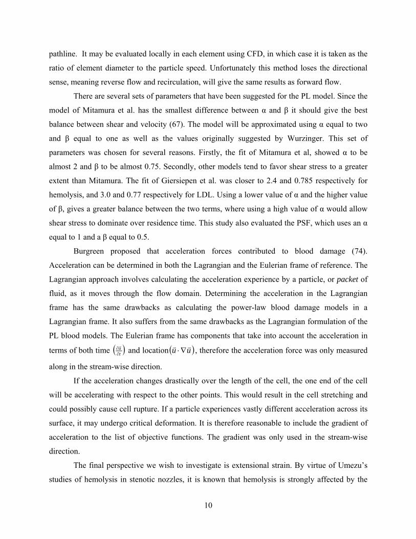
The PL models, summarized in Table 2, are based in the Lagrangian frame of reference.
The most common way of evaluating these damage indices (Di) is to integrate the value over the
streamline, using one of the following forms:
( )dtutADi
dtAdttADi
dttADi
T
T
T
∫
∫∫
∫
⋅∇+=
+=
=
−−
−−
−
vτατβτ
τατβτ
βτ
αβα
τ
βαβα
βα
11
11
1
.
8

Table 2: Fitted values for various power-law models for blood damage.
Reference:
Model Type
A α β
Giersiepen: Hemolysis 3.62e-5 2.416 0.785
Giersiepen: LDH 3.31e-6 3.075 0.77
Mitamura: Hemolysis 1.8e-6 1.99 0.765
Boreda et al.: PSF 1 1 0.452
Approximation: Hemolysis 1* 2 1
There are two problems with this approach. The first is that it assumes that RBCs do not
disturb the flow and that they always follow the path-lines. An extensive amount of research has
gone into fluid-particle flow and it is unlikely that the RBCs can be treated in this manner (70,
71). In fact, Karino and Goldsmith reported seeing platelets and RBCs migrating out of the
recirculation zone of a sudden expansion. The second problem with using streamlines is that the
results depend on the starting point of the particle. A large number of path-lines must be used in
order to get a statistically accurate measure of blood damage. Also, particles will not enter
stagnation zones without some form of stochastic modeling, or unless they a driven into it by
momentum.
An improvement to this would be to solve the flow in the Lagrangian frame of reference,
where the Di becomes a time varying parameter attached to each node of a FEM problem. This is
often difficult to do because it requires careful handling of the mesh in order to avoid element
inversion, low quality elements, and overly coarse meshes (72, 73).
Due to the current challenge in calculating the PL damage models; this thesis will adopt
an Eulerian frame of reference. This could be seen as a loss of accuracy, but it is also a way of
minimizing the Di over the whole fluid. Secondly, the shear stress tensor must be converted to a
scalar quantity, such as γμ & or maximum principal shear, as suggested previously. There are
other matrix norms such as the von Mises stresses, the octahedral stresses, wall shear stress, and
the Tresca criterion. But γμ & and the maximum principal shear are the two most commonly used
ones in fluid dynamics. Finally, the temporal component of shear history is estimated using the
residence time, which is the time required to traverse an specific distance along the flow
9
pathline. It may be evaluated locally in each element using CFD, in which case it is taken as the
ratio of element diameter to the particle speed. Unfortunately this method loses the directional
sense, meaning reverse flow and recirculation, will give the same results as forward flow.
There are several sets of parameters that have been suggested for the PL model. Since the
model of Mitamura et al. has the smallest difference between α and β it should give the best
balance between shear and velocity (67). The model will be approximated using α equal to two
and β equal to one as well as the values originally suggested by Wurzinger. This set of
parameters was chosen for several reasons. Firstly, the fit of Mitamura et al, showed α to be
almost 2 and β to be almost 0.75. Secondly, other models tend to favor shear stress to a greater
extent than Mitamura. The fit of Giersiepen et al. was closer to 2.4 and 0.785 respectively for
hemolysis, and 3.0 and 0.77 respectively for LDL. Using a lower value of α and the higher value
of β, gives a greater balance between the two terms, where using a high value of α would allow
shear stress to dominate over residence time. This study also evaluated the PSF, which uses an α
equal to 1 and a β equal to 0.5.
Burgreen proposed that acceleration forces contributed to blood damage (74).
Acceleration can be determined in both the Lagrangian and the Eulerian frame of reference. The
Lagrangian approach involves calculating the acceleration experience by a particle, or packet of
fluid, as it moves through the flow domain. Determining the acceleration in the Lagrangian
frame has the same drawbacks as calculating the power-law blood damage models in a
Lagrangian frame. It also suffers from the same drawbacks as the Lagrangian formulation of the
PL blood models. The Eulerian frame has components that take into account the acceleration in
terms of both time ( )tu∂∂v and location ( )uu vv ∇⋅ , therefore the acceleration force was only measured
along in the stream-wise direction.
If the acceleration changes drastically over the length of the cell, the one end of the cell
will be accelerating with respect to the other points. This would result in the cell stretching and
could possibly cause cell rupture. If a particle experiences vastly different acceleration across its
surface, it may undergo critical deformation. It is therefore reasonable to include the gradient of
acceleration to the list of objective functions. The gradient was only used in the stream-wise
direction.
The final perspective we wish to investigate is extensional strain. By virtue of Umezu’s
studies of hemolysis in stenotic nozzles, it is known that hemolysis is strongly affected by the
10
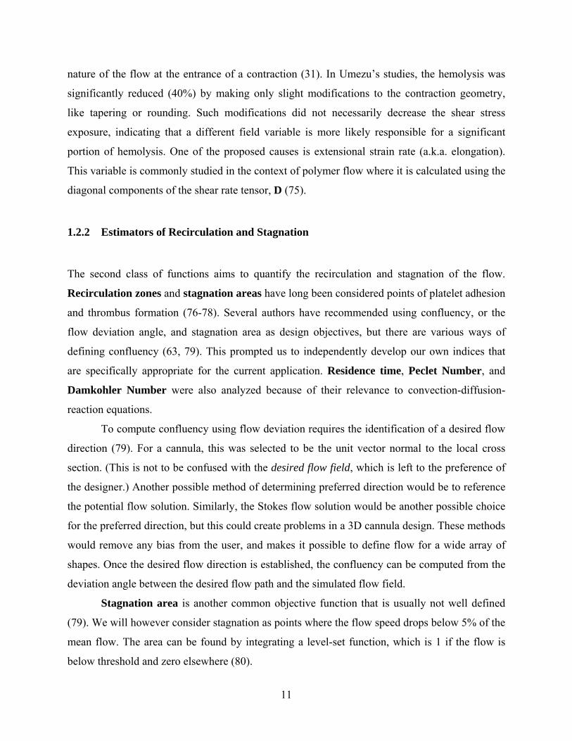
nature of the flow at the entrance of a contraction (31). In Umezu’s studies, the hemolysis was
significantly reduced (40%) by making only slight modifications to the contraction geometry,
like tapering or rounding. Such modifications did not necessarily decrease the shear stress
exposure, indicating that a different field variable is more likely responsible for a significant
portion of hemolysis. One of the proposed causes is extensional strain rate (a.k.a. elongation).
This variable is commonly studied in the context of polymer flow where it is calculated using the
diagonal components of the shear rate tensor, D (75).
1.2.2 Estimators of Recirculation and Stagnation
The second class of functions aims to quantify the recirculation and stagnation of the flow.
Recirculation zones and stagnation areas have long been considered points of platelet adhesion
and thrombus formation (76-78). Several authors have recommended using confluency, or the
flow deviation angle, and stagnation area as design objectives, but there are various ways of
defining confluency (63, 79). This prompted us to independently develop our own indices that
are specifically appropriate for the current application. Residence time, Peclet Number, and
Damkohler Number were also analyzed because of their relevance to convection-diffusion-
reaction equations.
To compute confluency using flow deviation requires the identification of a desired flow
direction (79). For a cannula, this was selected to be the unit vector normal to the local cross
section. (This is not to be confused with the desired flow field, which is left to the preference of
the designer.) Another possible method of determining preferred direction would be to reference
the potential flow solution. Similarly, the Stokes flow solution would be another possible choice
for the preferred direction, but this could create problems in a 3D cannula design. These methods
would remove any bias from the user, and makes it possible to define flow for a wide array of
shapes. Once the desired flow direction is established, the confluency can be computed from the
deviation angle between the desired flow path and the simulated flow field.
Stagnation area is another common objective function that is usually not well defined
(79). We will however consider stagnation as points where the flow speed drops below 5% of the
mean flow. The area can be found by integrating a level-set function, which is 1 if the flow is
below threshold and zero elsewhere (80).
11

Residence time is another factor that can be linked to thrombus deposition. A flow
region that is well “washed” will have low residence times and high clearance, while
recirculation zones will lead to infinite residence times and poor clearance. The residence time is
a Lagrangian variable, but will be estimated in the Eulerian frame of reference as the reciprocal
of fluid speed divided by characteristic length (e.g. element diameter). This approximation
eliminates directional dependence from the objective function.
Two common non-dimensional numbers, Peclet Number and Damkohler Number,
complete the set of objective functions studied in this research. These have not been used in the
literature for the optimization of blood-wetted devices. The Peclet Number is used in convection-
diffusion problems to measure the ratio of convection to diffusion. The Damkohler Number is
used in chemical processes to compare the rate at which reactions are occurring with the rate at
which the reactance are being removed from the area by convection, diffusion, or both.
Optimization of the flow path can only change the removal of reactants, so clearance caused by
diffusion is not used. These two indices naturally fit into the study of agonist-induced platelet
activation, platelet aggregation, and thrombus formation because all three phenomena have been
modeled as convection-diffusion based chemical reactions (4, 5, 81).
1.3 NUMERICAL METHODS FOR SOLVING PARTIAL DIFFERENTIAL
EQUATIONS
Conventional testing is time consuming and requires the construction of a prototype device,
which can be costly. It is possible to substitute live testing with numerical simulation in order to
avoid the construction of a prototype. Numerical simulations have been developed for
electromagnetics, fluid flow problems, structural analysis, convection-diffusion-reactions, heat
conduction, and other physical phenomena.
12
1.3.1 Finite Element Method
Shape optimization involves linking a numerical optimization algorithm with a partial
differential equation (PDE) solver. There are several methods for solving PDEs, but the most
popular methods are the Finite Difference Method (FDM), the Finite Volume Method (FVM),
and the Finite Element Method (FEM). Each method has its advantages and disadvantages, but a
detailed discussion of each method is beyond the scope of this work. The FDM is the simplest to
implement, but is not flexible enough for shape optimization since it does not readily conform to
curved boundaries. The FVM is more flexible, but has not gained wide field acceptance because
boundary condition can be difficult to implement. The FEM enjoys extensive use in most areas
including fluid dynamics, solid mechanics, and electromagnetism. FEM is also proven to be
efficient and accurate for solving fluid flows (82). Not only can the FEM conform to complex
boundaries, but FEM can also handle various boundary conditions.
1.3.2 FEM for Fluid Flow
The solution of fluid flow equation, particularly the NS equation, has been studied in great detail
(82). When solving NS-like equations including viscoelastic fluids, a mixed order Petrov-
Galerkin Method should be used for stability. To do this, the elements for velocity must be at
least one order higher than those for the pressure. If not, the method will not satisfy the
Ladyzhenskaya-Babuska-Brezzi (LBB) condition for stability. The standard Galerkin
method must be further stabilized, hence Petrov-Galerkin, in order to eliminate oscillation in
areas where the flow changes rapidly. This can be done using artificial viscosity as is done in the
FDM. The problem with this technique is that the actual equation is altered (82). Accuracy is
traded for stability. Stream-wise Diffusion Method (SWD) is better because it only increases the
viscosity along the streamline and not over the whole field. This does not smear the information
across the stream-lines where the gradients are usually highest as the AVM does (83, 84).
Unfortunately solution still may not be consistent with the original PDE, although it is more
accurate than the artificial viscosity method.
The concept of the SWD led to the Galerkin-Least-Squared Method (GLSM), which is
more precise (85, 86), and derived so that the FEM solution is consistent with the PDE. The
13
GLSM also includes variational terms relating to the pressure so the LBB condition is satisfied
automatically and equal order elements can be used to approximate the PDE. The drawback of
the GLSM is that it requires several adjustable parameters that are element-dependent and whose
physical meaning has not been determined.
Other methods try to decouple the pressure and velocity terms on order to satisfy the
LBB condition. The most popular approach is the Penalty Method (PM), which relaxes the
incompressibility condition, and replaces pressure with a penalty function of the divergence of
the velocity (82, 87). This method reduces number of unknowns down to just the velocity terms.
The PM does have several drawbacks. The first is that there is no accurate method for
determining the penalty function. This method does not calculate the pressure to the same
accuracy as the other methods. Finally, the coefficient matrix is nonsymmetrical and ill-
conditioned, which could lead to yet more errors and/or failure to converge to a solution (88, 89).
1.4 SHAPE OPTIMIZATION
Analyzing and entire design space in a systematic fashion would be difficult and time consuming
and costly to do with conventional prototyping or simulation. Design time can be reduced by
coupling numerical simulation to numerical optimization routines. This also allows for an
efficient search of the design space in order to find the best possible solution, assuming that the
goal or best design qualities is easily defined.
1.4.1 General Topics in Optimization
Optimization refers to a collection of methods for finding a set of parameters of a system that in
some way can be defined as optimal. Usually the parameters are determined by minimizing or
maximizing a function, called the objective function, which is some mathematical way of
measuring a goal, a value system, or desired design quality. One of the simplest examples of an
optimization technique is the least-square fitting. The objective function is the root mean square
14

of the difference between the data and the function being fitted, and the optimal parameters lead
to the best approximation. The standard form of an optimization problem is:
ul
e
e
n
xxx,...,mmi,Gi(x)
m, iGi(x)
RxxF
≤≤+=≤
==
∈
v
v
v
10,...,10
subject to
)(minimize
Most of the information presented in this section can be found in a standard text book on
optimization (90, 91), but specific references are places where they are needed or where they can
help clarify a technique.
Obtaining a solution efficiently and accurately depends on several factors, such as the
number of constraints, the number of design parameters, as well as the behavior of the objective
function and constraints. Finding the optima of linear and quadratic problem is uses well-
established methods. For non-linear or higher order problems (NLP) iterative techniques must be
implemented to find the optimum. Optimization routines are also broken down into
unconstrained and constrained optimization. Most techniques have been developed to deal with
unconstrained problems, so various methods are used to combine the constraints and the
objective function into a new objective function.
Several steps generally describe the standard optimization algorithms for the NLP. These
steps are determining a search direction, a line search, and evaluating the optimality of the new
point. These steps are repeated until the minimum or maximum are found. Most of the methods
for determining the search direction and doing the line search are LP or QP problems. The
following sections will discuss some of the most common algorithms for doing these sub-
problems, as well as the commonly used overall methods for optimization.
Converging to a global optimal point is difficult. Most routines will only find the global
minimum if the objective function and constraints are concave throughout the entire domain, or
if the initial conditions are specified close enough to the global minimum. Therefore, it is
common repeat the optimization several starting points. This usually allows the solver to find a
global optimum, although there are no guarantees that this is the case.
The final topics that will be discussed are common methodologies for dealing with
constraints, multi-objective optimization, and the formulation of the optimization for PDE
15
constrained problems. For the interest of space, optimization topics that are not relevant to the
current project will be omitted here, including genetic algorithms and discrete point optimization
methods. The ensuing optimization methods will be discussed in terms of a minimization
problem, which tends to be standard procedure. Maximization routines can apply the same
techniques with slight modifications, but a maximum can be determined by minimizing the
negative of the objective function\
1.4.1.1 Determining the Search Direction
The first step in most optimization routines is to determine a search direction. These
algorithms use gradient information to determine the general direction toward the minimum. The
simplest gradient-based method that is commonly used to find the search direction is called the
steepest decent. The search direction, p, is the negative of the gradient, since the gradient points
in the direction of maximum increase. This algorithm is guaranteed to converge and does so
linearly. However, in the case that an objective function is elongated in a particular parameter
direction the convergence is slow, and can take a large number of iterations to converge.
A more sophisticated method for determining the search direction is based on Newton’s
Method for root finding. The optimal point of a function f is defined as where the gradient is
zero, and so Newton’s equation, given by
pHf v=∇− ,
where H is the Hessian matrix, and p is the search direction. This method has the advantage that
it shows quadratic convergence around the optimal point yet does not suffer the problems
associated with steepest descent. But, unlike the steepest descent method, the Newton’s method
is not guaranteed to converge. This method will find a search direction toward the nearest
optima, whether it is a minimum, a maximum, or a saddle point. If the Hessian matrix, H, is
positive definite, then the routine will head in the direction of a local minima. Positive
definiteness implies that:
00 ≠∈∀> nT RxAxx .
Several techniques have been developed in order to deal with situations where the
Hessian is not positive definite. The simples method is to use the steepest descent until the
Hessian becomes positive definite. This method gives rapid convergence near the optimum, but
has all of the drawbacks of the steepest descent method. The second method is called the Picard
16

Method, where the Hessian is only approximated. Components of the Hessian that could lead to
it becoming negative or indefinite are dropped. This method does not show the quadratic
convergence as Newton’s Method, but it does not suffer the drawbacks of the steepest descent
method. However, Picard's method requires that the Hessian be calculated mathematically which
is not always possible. Other methods for approximating the Hessian in a manner that keeps it
positive definite can also be used. These will be discussed a little later in more detail.
The preceding discussion has not mentioned how the gradients and Hessian are obtained.
Ideally, the best results occur if the gradients can be calculated directly through differentiation or
variational calculus, but most practical problems do not lend themselves readily to
differentiation. In this case the derivative can be calculated using finite differences, which
involves perturbing each optimization parameter slightly. This can be difficult because the
truncation error can adversely affect the optimizer. In some cases the numerical noise can set up
local minima or numerical oscillations, which cause difficulties in convergence. Also,
numerically calculating the derivative can be computationally expensive for large problems such
as those using CFD or other PDEs.
The Hessian matrix would require additional function evaluations in order to use finite
differences to determine its values (92). The problem with numerical differentiation is that it
quickly becomes noisy and so higher derivatives become less and less accurate. Even if the
Hessian is reasonably approximated using finite differences, there is no guarantee that the matrix
will be positive definite. Therefore the Hessian is usually approximated using more sophisticated
the methods described by Broyden (93), Fletcher (94), Goldfarb (95), and Shanno (96) called
BFGS. This method uses the values of the function, as well as the derivative information (either
exact or approximated), to build up the curvature information. The Hessian is initially set to a
positive definite matrix, such as the identity matrix, and is updated at each iteration using the
equation:
kkk
kkk
kkTk
kkTk
Tk
kTk
Tkk
kk
ffqpxxs
wheresHsHssH
sqqq
HH
∇−∇==−=
−+=
+
+
+
1
1
1 ,
vα
17

This method guarantees that the Hessian will remain positive definite. It is also possible to
update the inverse of the Hessian using a similar method so that the search direction can be
found without a matrix inversion (97, 98).
The Newton-based methods usually involve finding the search direction using an iterative
method. It is often the case, that only a few iterations are used to determine p, to reduce
computational time.
1.4.1.2 The Line Search
A line search takes place once an appropriate search path is found in order to determine
how far to move along the search direction. It is another minimization sub-problem, except that
the function is only minimized along a single direction in the form:
)( pxF vv α+
where α is a constant chosen to strike a balance between convergence and stability.
Several methods are used that reduce the time spent in this subroutine; just as the search
direction was modified to save time. The first method is an interval halving method, where α is
set to 1 for the initial step. The function is evaluated and checked to see if it decreased a
sufficient amount. If the function does not decrease sufficiently, the step size is halved until the
required reduction occurs. If the step-size becomes too small, the routine fails. This commonly
occurs if the angle between the search direction and the contour line is small. More advanced
methods use quadratic approximations, cubic approximations, or a mixture of both to find a
minimum faster. The minima of these functions can be found analytically, and allow for α to be
extrapolated beyond 1. Normally, extrapolation is numerically undesirable, but if the
extrapolated point does not reduce the function, it increases the range over which alpha can be
interpolated.
1.4.1.3 Evaluating Optimality
The optimality condition is ultimately defined where the gradient of the objective
function is zero or at the lowest value along in the domain. In practice, an optimality condition
may be defined by the gradient below a small threshold value. This is a relatively straightforward
calculation. First, the gradient of the new point is calculated, which will also be used in the next
Newton step if the point is not optimal. The second step is to evaluate the norm of the gradient,
18

which should be zero at the optimum. For a constrained problem, the minimum might be outside
of the allowable parameter range. In this instance the point along the boundary with the lowest
value is the minimum.
1.4.1.4 Handling Constraints in Optimization Problems
The routines for finding optimal values are developed for unconstrained problems, but
most problems are constrained in some fashion. A problem is constrained if there are restrictions
on the values that the optimization parameters can assume. Most engineering problems are
constrained by logic, user requirements, physical principles or limits, or other practical issues.
Constraints can take on various forms such as bounds on certain parameters or nonlinear and
linear relationships – often represented by auxiliary equations. Equality constraints actually
reduce the size of the problem, since one parameter can always be expressed in terms of the
others. Constraints also help improve the convergence qualities of the optimization routines.
In constrained optimization, the problem must be transformed into a new unconstrained
formulation using various methods. Early methods involved developing penalty functions that
would increase rapidly as the parameters came close to violating the constraints. More modern
methods have been developed using Lagrange multipliers, since these early methods were
inefficient, difficult to implement, and altered the design space. The problem would now be
considered unconstrained, but with steep penalties for violating the constraints, hence driving the
solution back into the feasible region.
1.4.2 The Sequential Quadratic Programming Method for Optimization
The favored gradient-based method for unconstrained optimization is the Quasi-Newton method.
This method builds up the curvature information at each step, and uses it to approximate the
objective as:
)(xFcxfHxx TT v=+∇+ .
The method typically uses the BFGS to update the Hessian, but other methods can also be used.
The line search is done using a mixed quadratic and cubic line search method.
19

SQP is the most efficient, accurate, and successful version of constrained optimization
routines (99). This method closely follows the Newton’s method for constrained problems (100-
102). The SQP method rewrites the constrained problem into the form:
⎩⎨⎧
>=
+= ∑=
Violated Constraint0ednot violat Constraint0
)()(),(1
λ
λλ
where
xGxFxLm
iiivvv
using the Lagrange multiplier method. The Hessian for L is updated using the quasi-Newton
approach.
1.4.3 Multi-Objective Optimization
Although single objective optimization can produce good working models, it is often impractical.
Real-life design problems almost always involve multiple and competing goals, such as the
present study wherein several indices are used to evaluate blood damage. Usually the objective
function is represented by a vector of objectives, but the problem with this formulation is that the
tradeoff between each objective function is not known a priori. In fact, no unique solution can be
found for MOO; only a range of solutions can be determined, depending on the weighting
applied to each function.
The MOO problem can be stated in the same fashion as the unconstrained problem,
except now the objective function is a vector. When there is not a unique solution to the MOO
the objective function should be analyzed using Pareto optimality (103, 104). Here the MOF
refers to the combination of all objective function, while OF will refer to each individual
function. Strong Pareto optimality occurs when at least one OF is at a minimum when the MOF
is at a minimum. Weak Pareto optimization is where the MOF is at a minimum, but none of the
OFs are actually at a minimum (105). Pareto optimality is characterized by the concept of
noninferiority. A noninferior solution is where improvements to one OF requires a degradation
of another function (103, 104).
The first step in MOO is to transform the OF through normalization. This prevents any
single function from dominating the others based only on its magnitude. The simplest
20

transformation, which will be referred to as KS transformation in this thesis, was presented by
Koski and Silvenoinen (106):
minFFF inorm
i = ,
which normalizes the OFs so that their value reaches unity at their optimal points. Koski
previously presented a second method (106, 107):
minmax
min
ii
iinormi FF
FFF
−−
= ,
which normalizes for both magnitude and variation. This transformation, referred to in this thesis
as the Koski transformation, is normalized from 0 to 1. These second step is to determine the
relationship between the OFs. The MOF can formed using numerous techniques, but the most
basic is the weighted sum method (105):
∑=N
normiiFwMOF .
There are many methods for the selection of the weights in order to avoid arbitrary selection
(105). Most of these methods involve ranking the OFs in order of their importance, but for this
thesis each form of blood damage will be given a weight of 1, meaning none has a higher priority
than the next. After the MOF is determined, the problem is ready for any standard optimization
routine.
1.4.4 Shape Optimization in Fluid Dynamics
Shape optimization of a PDE problem has a similar structure to a standard optimization problem.
The general form the problem is given by:
MmiGimiG
uC
rwuF
e
ei
,...,0)(,...,10)(
0),(:by dConstraine
/),(min
=≤==
=
πππ
ππ
v
v
vv
v
vv
Here the weak form of the PDE is treated as an additional constraint on the problem, and uv
refers to the solution of that PDE. The PDE is solved for a given set of shape parameters and the
21

solution is used to calculate the OF. Since a PDE is a spatial problem, the OF will be calculated
as the norm of the function relating to blood damage. Three norms will be considered for this
study and are defined as:
Norm. Average:)(
)(
NormInfinity :))(max()(
Normn Integratio:)()(
∫
∫
∫
Ω
Ω
∞
Ω
Ω
Ω=
Ω=
Ω=
d
dxfxf
inxfxf
dxfxf
a
i
v
v
vv
vr
Derivatives for the PDE constrained problem are not well defined. Most algorithms rely on finite
difference approximations of gradients, and use an approximate Hessian using BFGS or the like.
Two other methods are for determining the gradients are sensitivity analysis. Sensitivity analysis
use calculus of variations for determine the sensitivity of the OF to a design variable, which
includes a sensitivity of the flow variables to the design variable. The sensitivity analysis of the
weak form of the PDE is used to find the sensitivity of the flow variables. This method is faster
that a finite difference method because the sensitivity equations are linear, where the NS
equations are non-linear. Unfortunately this technique requires some method of determining the
sensitivity of the PDE to the shape parameter, which may be difficult to define.
22

2.0 METHODS
This study focused on the optimization of a two-dimensional fluid dynamic domain
representative of a blood conduit, or cannula. The domain was comprised of a 90 degree arc (or
“elbow”) with prescribed boundary conditions, including a flow rate requirement of 6 liters per
minute.
2.1 NUMERICAL METHODS
2.1.1 Computational Fluid Dynamics Using FEMLAB
All simulations in this study were performed using FEMLAB (COMSOL, Inc.), a multiphysics
finite element analysis package. The simulations were run with Taylor-Hood finite elements:
quadratic in velocity and linear in pressure. The mesh elements were triangular in 2-D and
tetrahedral for 3D. The mesh was refined until it was fairly dense, approximately 4,000-5,000
elements. A continuation method for flow rates starting at zero and increasing up to 6 L/min was
used to ensure stable conversion. The non-linear tolerance was of the order –4 for the early
continuation steps, but was increases to –7 for the final step. This helped to reduce the
computational time, without decreasing the accuracy of the scheme.
The inlet boundary condition was prescribed by an uniform velocity profile, indicative of
the entrance flow from the heart. The outlet condition was set to zero traction (pressure of 0
dynes/cm2) and with a tangent constrained normal to the exit plane. The blood was treated as a
Newtonian fluid with a viscosity of 3.5 cP and a density of 1.05 g/cm2. This is the commonly
used asymptotic value for blood at room temperature. It has been shown that simulations using a
Newtonian approximation can be quite accurate when the Reynold’s number is sufficiently large
23

and the blood viscosity is taken at an average shear rate for the flow (74). The viscoelastic
properties of blood were ignored because they usually occur at very low shear rate (<2/s) and the
shear rate of this study was several orders higher (> 200/s).
2.1.2 Optimization Using the SQP Method
The optimization was performed in several steps. The first step was to minimize and maximize
each of the individual objective functions for the 2-D cannula. Two multi-objective optimization
methods were then evaluated in order to determine the best method to combine the objective
functions. The optimization was done using the SQP method, which is built into the optimization
toolbox of MATLAB (by Mathworks). When needed, the maximum was found by minimizing
the negative of the objective function, since the SQP method only solves for minimums. The
optimization routine was started at several different points in order to find the global minimum.
These starting points included the minimum and maximum values from the design space analysis
in 2-D. The convergence rate, optimum values, and shapes were analyzed for design
characteristics.
2.2 ANALYZING OBJECTIVE FUNCTIONS
2.2.1 Qualitative Analysis of Objective Functions
Prior to performing the actual shape optimization, a rigorous evaluation and comparison of the
objective functions was performed by simulating flow in two-dimensional channels that have
been selected for particular flow behavior. Although it is possible to get a numerical comparison
of each shape, the primary focus will be to observe behavior of the blood damage functions in
each flow field. Both good quality (low shear and no recirculation) and bad quality designs were
selected (Figure 1). The first good cannula was designed using the upper right quadrant of a ring,
24

while the second came from the preliminary results of the 2-D optimization for the Peclet
Number.
Figure 1: Flow through selected cannula plotted with pressure contours and velocity vectors.
Several other designs were chosen because of the poor flow features that they generate,
such as zones of high stress and recirculation. The most obvious of the bad designs, was a
cannula that has been “pinched off” at its center, thereby throttling the flow. Figure 2 shows the
recirculation zones in the bad cannula designs. The flow of blood in a stenosis has been studied
extensively (108-111), and it is known to cause a high rate hemolysis at the throat and thrombus
formation downstream of the contraction where a recirculation region forms. A pinched cannula
behaves in a similar manner as a stenosis. The 90o cannula develops two recirculation regions.
The first is in the upper right corner and the second one is located on the inner wall just distal to
the turn. These two recirculation zones act to constrict the flow through this section and cause a
jet similar like the stenosis, but weaker. Another poor feature of the square cannula is that there
is a zone of high stress that forms just before the turn on the lower wall.
25

Figure 2: Recirculation regions of bad cannula designs
The two more bad designs were analyzed in this part of the study. The third bad cannula
design is based on the preliminary optimization results for vorticity. In order to reduce the
vorticity, the walls expand to reduce velocity, which produces a large recirculation zone along
the inner wall. The final bad design is not physically accurate, but is a purely mathematical
model that provides useful intuition into the objective functions. The inlet and outlet are placed
in position for the inflow cannula of the Streamliner VAD, and the walls were composed of
straight lines. The flow is forced to turn quickly upon entering and exiting the cannula, which
results in high shear stresses along the walls.
The flow field was calculated for each cannula using CFD. The velocity vector field and
the pressure field of each flow were plotted in order to verify the flow each channel. Once this
was done, the objective functions were analyzed in several ways. The damage functions were
plotted over the entire domain and visually compared to see how they identified important flow
features. Secondly the objective functions were analyzed using all three norms and the results
were tabulated and compared by ranking the designs.
26
2.2.2 Quantitative Analysis of Objective Functions
Although the qualitative analysis of objective function is insightful, it is more desirable to do a
more rigorous mathematical comparison of the objective functions. This was done in several
steps. The first step was to analyze the design space that was selected for the optimization of the
2-D cannula. The correlation between various objective functions can then be made using the
resulting data set. It is possible to determine whether objective functions are independent, by
studying the correlation matrix. The second step was to use principal component analysis to
determine the number of objective functions that are necessary to reasonable describe all modes
of blood damage. Statistical analysis was used to mathematically analyze the behavior of the
objective functions, in order to determine the variance over the design space and to estimate
robustness of the function. Calculus of variations was used to determine the convergence
characteristics of some of the objective functions in order to determine if they would be suitable
to use in standard optimization routines.
In order to compare the objective functions in a more mathematical way, we examined
the design space for the 2-D cannula. The design-space is composed of all possible
conformations that the shape can assume. In this analysis we discretized the design space into
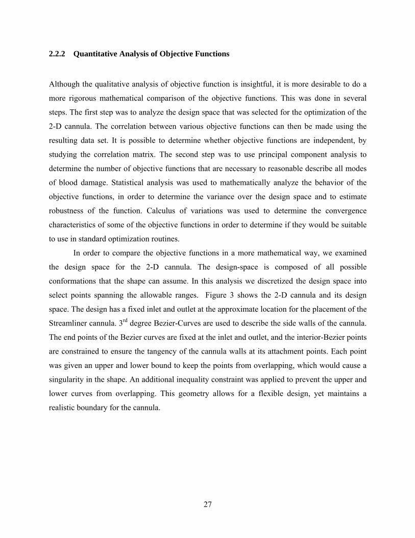
select points spanning the allowable ranges. Figure 3 shows the 2-D cannula and its design
space. The design has a fixed inlet and outlet at the approximate location for the placement of the
Streamliner cannula. 3rd degree Bezier-Curves are used to describe the side walls of the cannula.
The end points of the Bezier curves are fixed at the inlet and outlet, and the interior-Bezier points
are constrained to ensure the tangency of the cannula walls at its attachment points. Each point
was given an upper and lower bound to keep the points from overlapping, which would cause a
singularity in the shape. An additional inequality constraint was applied to prevent the upper and
lower curves from overlapping. This geometry allows for a flexible design, yet maintains a
realistic boundary for the cannula.
27

Figure 3: Design space for the 2-D cannula.
The design space was discretized by dividing the range for each parameter into six points
and removing any point combination that violates the inequality constraint. The flow was solved
for each set of discrete points. MATLAB was then used to determine the correlation between
each objective function and to do the principal component analysis (PCA). The eigenvalues of
PCA can help determine how many function provide distinct information to a system. If two
functions are highly correlated, then one function can be used to represent the other so one
function can be dropped. MATLAB was also used to calculate the statistics: mean, median,
maximum, minimum, and the variation; and to plot the histogram for each objective. The
histograms will tend to be skewed left or right if there is a large difference between the mean and
the median. The skew is indicative of the curvature of the objective function around the optimal
value. For example if the distribution is skewed toward the optimal value; that point is relatively
flat and robust. If the distribution is skewed away from the optimal point; that point is sharply
curved and very sensitive to small design changes.
2.3 OPTIMIZATION OF A 2-D CANNULA
While it is the ultimate objective to optimize the design of a blood cannula in three-dimensions,
this study adopted a two-dimensional simplification for several reasons. The most obvious
28

motivation is because of dramatically reduced computational time thereby allowing more
simulations to be performed in a practical span of several months. The additional speed also
enables insight to the sensitivities and behaviors of the objective functions upon the optimum
shape. The methods that were developed and refined in this two-dimensional analysis can be
readily expanded to 3D.
The characterization of the geometry is crucial for determining the best design. Although
the method for describing the 2-D geometry described in the previous section only has four
degrees of freedom, this should be sufficient for this problem. The SQP method (described in
4.3.3) was used to perform both the single-objective optimization and the multi-objective
optimization. Each objective function was individually optimized in order to analyze its effect on
the geometry, but also so that these values could be used in the multi-objective optimization
problem. The Koski approach was applied to the multi-objective optimization because it
normalized both the magnitude and variation of the function, which gives each objective function
equal footing.
The optimal designs were analyzed visually by observing the general trend in the shape.
The flow within the cannula was also checked for flow features, but also by examining the other
objective functions. The multi-objective design was also analyzed in order to find out the percent
difference between the optimal design and the MOO design. This is an estimate of how much
performance is “lost” from each objective in order to accomplish the multi-objective
optimization.
29

3.0 RESULTS OF OBJECTIVE FUNCTION ANALYSIS
It is important to understand the behavior of each function as it pertains to quality and low
quality designs. It is also important to have and indication of the ability of each function to
indicate flow regions that would cause increased blood damage. The following experiments
determine which functions provide the best information for use in a multi-objective optimization
problem.
3.1 QUALITATIVE ANALYSIS OF OBJECTIVE FUNCTIONS
The CFD solutions for the flow fields provide good insight into the flow through each cannula.
Figure 1 shows the flow features for each cannula. The CFD results confirm that there are
recirculation regions in the 90o turn, the minimum-vorticity cannula, and the pinched cannula.
The elevated shear stress can be seen in the straight cannula, the 90o turn, and the pinched
cannula. The jet regions are also apparent in the pinched cannula and the 90o turn. There are also
high stress regions at the inlets, which are a result of the rapid deceleration of the flow at the
inlet. This indicates that a better boundary condition would be advisable, but the inlet flow for a
cannula is typically blunted and not fully developed.
The features found when plotting the objective functions describing hemolysis and shear
induced platelet activation had similar features. The actual magnitude of the plots varied, but the
similarities were distinctive. Figure 4 shows six of these functions, plotted in the 90o cannula.
Some of the features that are prominent are the contracted regions showing the boundary layer
formation and the boundaries of the recirculation regions.
30

Figure 4: Field plot of the several functions that represent shear induced hemolysis.
Most of the functions relating to recirculation and stagnation failed to catch all of these
features, particularly those just distal to the contraction in the pinched cannula and the inner wall
of the square cannula. (See Figure 5) The flow angle clearly shows the presence of all of the
recirculation zones. Peclet number, residence time, and stagnation area all fail to identify these
recirculation zones because the speed of the recirculation is high in these two regions. The
residence time is slightly larger in the recirculation zone (100.75), but is not very distinct when
compared to the boundary layer (104). Stagnation area only shows the regions where there is a
boundary between forward and backwards flow. At best, these functions show the boundary
between forward and backwards flow, but they do not show the entire area as well as the
deviation angle. The vorticity function can pick up these high-speed zones, but fails to pick up
slow recirculation cells, like the one that forms in the minimum-vorticity cannula.
31
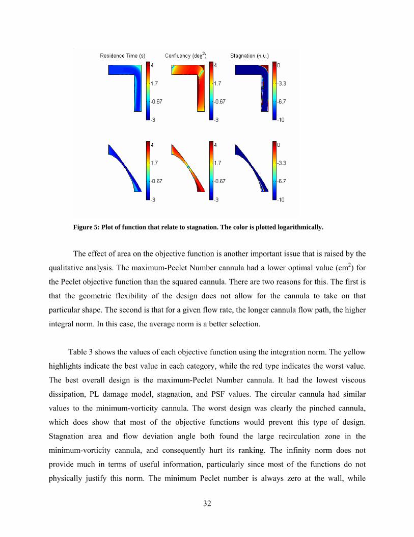
Figure 5: Plot of function that relate to stagnation. The color is plotted logarithmically.
The effect of area on the objective function is another important issue that is raised by the
qualitative analysis. The maximum-Peclet Number cannula had a lower optimal value (cm2) for
the Peclet objective function than the squared cannula. There are two reasons for this. The first is
that the geometric flexibility of the design does not allow for the cannula to take on that
particular shape. The second is that for a given flow rate, the longer cannula flow path, the higher
integral norm. In this case, the average norm is a better selection.
Table 3 shows the values of each objective function using the integration norm. The yellow
highlights indicate the best value in each category, while the red type indicates the worst value.
The best overall design is the maximum-Peclet Number cannula. It had the lowest viscous
dissipation, PL damage model, stagnation, and PSF values. The circular cannula had similar
values to the minimum-vorticity cannula. The worst design was clearly the pinched cannula,
which does show that most of the objective functions would prevent this type of design.
Stagnation area and flow deviation angle both found the large recirculation zone in the
minimum-vorticity cannula, and consequently hurt its ranking. The infinity norm does not
provide much in terms of useful information, particularly since most of the functions do not
physically justify this norm. The minimum Peclet number is always zero at the wall, while
32

maximum stagnation is always one when flow is below threshold. The infinity norm can be used
for the shear dependent objective functions.
Table 3: The evaluation of each objective function in the selected designs.
Cannula Selections
Objective Function
Good
Cannula
Direct
Cannula
Squared
Cannula
Minimum
Vorticity
Pinched
Cannula
Maximum
Peclet #
Vorticity 4.16E+05 1.59E+06 8.66E+05 2.78E+05 1.68E+07 9.39E+05
Viscous Dissipation 9.61E+04 1.44E+06 1.54E+05 5.59E+04 4.96E+06 1.91E+04
Damage Function 1 6.43E+07 1.60E+09 5.88E+07 2.57E+07 2.35E+09 1.02E+06
Damage Function 2 1.28E+08 3.19E+09 1.17E+08 5.12E+07 4.71E+09 2.04E+06
Damage Function 3 1.22E+7 2.93E+08 1.11E+07 4.84E+06 4.35E+08 1.96E+05
Residence Time 3.32E+03 1.40E+03 2.35E+03 2.74E+03 1.19E+03 1.25E+03
Acceleracton 5.41E+06 6.83E+08 2.36E+07 2.27E+07 1.18E+10 2.48E+07
Gradient of
Acceleration 1.84E+17 2.04E+25 3.13E+18 1.46E+20 6.42E+26 3.51E+20
Stagnation Area 3.34E-01 1.41E-01 7.60E-01 1.01E+00 1.33E-01 1.25E-01
Flow Direction 1.93E+01 4.42E+03 2.98E+04 3.63E+04 1.20E+04 1.55E+02
Maximum Shear
Stress 5.99E+05 2.86E+06 9.62E+05 3.46E+05 3.10E+07 1.17E+06
Elongation 9.15E+04 6.35E+05 4.78E+04 3.43E+04 7.08E+06 1.15E+05
Peclet Number 4.55E+11 4.17E+11 5.78E+11 4.80E+11 4.43E+11 4.76E+11
Damkohler Number 8.26E+00 8.14E-02 6.30E+00 8.71E+00 5.65E-02 4.43E+00
PSF 4.39E+03 1.06E+04 2.76E+03 1.72E+03 1.31E+04 2.83E+02
3.2 QUALITATIVE ANALYSIS OF THE DESIGN SPACE
3.2.1 Evaluation of the Design Space
Table 4 shows the correlation matrix for the design space using the integral norm approach.
Numbers in blue type indicate high correlation values, red type indicates moderately anti-
correlated values, and yellow highlights indicate the diagonal of the matrix. 1249 solutions were
required to cover the entire space. The functions that have been linked to hemolysis did show
33

high correlation with each other (C>0.95). The platelet stimulation function also showed a
reasonable correlation to the other power-law damage models (C>0.8). This was surprising since
the PSF is approximately the square root of the hemolysis model. The correlation between the
damage function using the maximum principal shear stress and the index based on viscous shear
stress indicated that they were virtually equivalent. The acceleration force was found to correlate
to the hemolysis models, but not as well as amongst each other (0.93>C>0.92 to >0.99). There
were no anti-correlated functions (C<-0.75). This means that there are no one-to-one trade offs in
the objective functions, so is possible to improve all of the objective functions to some extent.
Peclet Number, stagnation area, confluence, and the Damkohler Number all appear to be
independent of the each other and the other functions. The gradient of acceleration, although
capable of determining jet flow, does not correlate with the various hemolysis models. This
means that it is unlikely that this function actually contributes significantly to hemolysis.
Table 4: Correlation table for the design space analysis.
Ref.
frame Vorticity
Viscous
Dissipation
Damage
Function 1
Damage
Function 2
Damage Function 3
Res.
Time
Vorticity Both 1.0000 0.9996 0.9981 0.9981 0.9981 -0.3948
Viscous Dissipation Both 0.9996 1.0000 0.9979 0.9979 0.9977 -0.3924
Damage F1 Lag 0.9981 0.9979 1.0000 1.0000 1.0000 -0.3759
Damage F2 Lag 0.9981 0.9979 1.0000 1.0000 1.0000 -0.3759
Damage F3 Lag 0.9981 0.9977 1.0000 1.0000 1.0000 -0.3770
Residence Time Lag -0.3948 -0.3924 -0.3759 -0.3759 -0.3770 1.0000
Acceleraction Both 0.9278 0.9359 0.9259 0.9258 0.9238 -0.3193
Gradient of Accel Both 0.7298 0.7455 0.7259 0.7255 0.7220 -0.1879
Stagnation Area Eul -0.1076 -0.1049 -0.0984 -0.0984 -0.0993 -0.0597
Confluency Both 0.4360 0.4330 0.4472 0.4472 0.4478 -0.2814
Principal Shear Stress Both 0.9996 1.0000 0.9979 0.9979 0.9978 -0.3925
Elongation Both 0.9982 0.9995 0.9968 0.9968 0.9964 -0.3893
Peclet Number Both 0.0926 0.0879 0.1120 0.1120 0.1117 0.3702
Damkohler Number Both -0.2024 -0.1951 -0.1781 -0.1782 -0.1803 -0.1194
Platelet Stim. Funct. Both 0.8178 0.8040 0.8063 0.8065 0.8099 -0.3408
34

Table 4 (continued from left side)
Accel-
eration
Gradient
of Accel-
eration
Stagnation
Area
Conflu-ency
Principa
l Shear
Stress
Elong-
ation
Peclet Number
Damkohle
r Number PSF
0.9278 0.7298 -0.1076 0.4360 0.9996 0.9982 0.0926 -0.2024 0.8178
0.9359 0.7455 -0.1049 0.4330 1.0000 0.9995 0.0879 -0.1951 0.8040
0.9259 0.7259 -0.0984 0.4472 0.9979 0.9968 0.1120 -0.1781 0.8063
0.9258 0.7255 -0.0984 0.4472 0.9979 0.9968 0.1120 -0.1782 0.8065
0.9238 0.7220 -0.0993 0.4478 0.9978 0.9964 0.1117 -0.1803 0.8099
-0.3193 -0.1879 -0.0597 -0.2814 -0.3925 -0.3893 0.3702 -0.1194 -0.3408
1.0000 0.9030 -0.0562 0.3678 0.9353 0.9434 0.0650 -0.0867 0.5889
0.9030 1.0000 -0.0308 0.2222 0.7441 0.7605 0.0848 -0.0338 0.3286
-0.0562 -0.0308 1.0000 0.6913 -0.1051 -0.1020 -0.0476 0.6907 -0.2559
0.3678 0.2222 0.6913 1.0000 0.4331 0.4293 -0.0352 0.3848 0.3145
0.9353 0.7441 -0.1051 0.4331 1.0000 0.9995 0.0883 -0.1956 0.8047
0.9434 0.7605 -0.1020 0.4293 0.9995 1.0000 0.0829 -0.1873 0.7883
0.0650 0.0848 -0.0476 -0.0352 0.0883 0.0829 1.0000 0.0030 0.0643
-0.0867 -0.0338 0.6907 0.3848 -0.1956 -0.1873 0.0030 1.0000 -0.4925
0.5889 0.3286 -0.2559 0.3145 0.8047 0.7883 0.0643 -0.4925 1.0000
The principal component analysis yielded eigenvalues that were ranked from the lowest to
highest as shown in Figure 6. The bottom half of the figure shows the individual percent in blue,
and the cumulative percent in red. The cumulative percentages indicate that only three to four of
the objective functions represent more than 90% of the overall information represented by the
correlation matrix. It is statistically acceptable to use only four out of 15 for the optimization
method. Although four functions should be used to reach 90% of the information, three should
be sufficient, since the gradient of acceleration does not appear to correlate with hemolysis.
35

Figure 6: Plot of the eigenvalues and their information percent.
The correlation matrix for the infinity norm and the average norm were also evaluated.
There were no strong correlations among the objective functions evaluated by the infinity norm,
except for the PL models. They also showed little correlation to the equivalent function
evaluated with the integral norm. This is most likely because these are evaluated at a single point
in the flow field, where the integral and average norms are evaluated over the entire flow field.
Integrals tend to smooth out noisy data. The correlation matrix for the average norm showed
similarities to that of the integral norm. This is because the ratio between each function does not
change with the norm.
More statistical information can be gathered from the design space study. Table 5 shows
the minimum and maximum of the integral norm, the mean and medium of integral norm, and
the variance of the design space. Almost all of the functions had a variance of 4-6% and several
orders of magnitude difference between their max and min values. The only objective functions
that had a lower variance were residence time (0.13%), stagnation area (1.37%), Peclet Number
(0.06%), Damkohler Number (2.22%), and the PSF (1.43%). The acceleration force and the
gradient of acceleration both had high variances, 17.03% and 65.9% respectively.
36
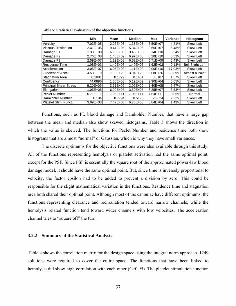
Table 5: Statistical evaluation of the objective functions.
Min Mean Median Max Varience HistogramVorticity 7.03E+05 2.23E+06 1.35E+06 7.50E+07 4.81% Skew LeftViscous Dissipation 2.41E+05 9.41E+05 5.34E+05 3.66E+07 5.48% Skew LeftDamage F1 1.38E+08 6.98E+08 3.48E+08 3.14E+10 6.54% Skew LeftDamage F2 2.76E+08 1.40E+09 6.97E+08 6.28E+10 6.53% Skew LeftDamage F3 2.59E+07 1.29E+08 6.52E+07 5.71E+09 6.43% Skew LeftResidence Time 1.08E+03 1.40E+03 1.40E+03 1.62E+03 0.13% Bell Slight LeftAcceleraction 3.05E+07 6.06E+08 1.11E+08 9.00E+10 17.03% Skew LeftGradient of Accel 4.58E+19 7.98E+23 3.04E+20 5.68E+26 65.89% Almost a PointStagnation Area 0.1091 0.1729 0.1461 0.6107 1.37% Skew LeftConfluency 44.0896 1.58E+03 5.12E+02 2.90E+04 5.65% Skew LeftPrincipal Shear Stress 9.20E+05 3.61E+06 2.05E+06 1.40E+08 5.47% Skew LeftElongation 1.05E+05 6.90E+05 3.50E+05 3.25E+07 6.53% Skew LeftPeclet Number 6.71E+11 7.06E+11 7.06E+11 7.54E+11 0.06% NormalDamkohler Number 0.104 0.7794 0.5193 2.9824 2.22% Skew LeftPlatelet Stim. Funct. 3.09E+03 7.47E+03 6.73E+03 3.84E+04 1.43% Skew Left
Functions, such as PL blood damage and Damkohler Number, that have a large gap
between the mean and median also show skewed histograms. Table 5 shows the direction in
which the value is skewed. The functions for Peclet Number and residence time both show
histograms that are almost “normal” or Gaussian, which is why they have small variances.
The discrete optimums for the objective functions were also available through this study.
All of the functions representing hemolysis or platelet activation had the same optimal point,
except for the PSF. Since PSF is essentially the square root of the approximated power-law blood
damage model, it should have the same optimal point. But, since time is inversely proportional to
velocity, the factor epsilon had to be added to prevent a division by zero. This could be
responsible for the slight mathematical variation in the functions. Residence time and stagnation
area both shared their optimal point. Although most of the cannulae have different optimums, the
functions representing clearance and recirculation tended toward narrow channels; while the
hemolysis related function tend toward wider channels with low velocities. The acceleration
channel tries to “square off” the turn.
3.2.2 Summary of the Statistical Analysis
Table 4 shows the correlation matrix for the design space using the integral norm approach. 1249
solutions were required to cover the entire space. The functions that have been linked to
hemolysis did show high correlation with each other (C>0.95). The platelet stimulation function
37
also showed a reasonable correlation to the other power-law damage models (C>0.8). This was
surprising since the PSF is approximately the square root of the hemolysis model. The
correlation between the damage function using the maximum principal shear stress and the index
based on viscous shear stress indicated that they were virtually equivalent. The acceleration force
was found to correlate to the hemolysis models, but not as well as amongst each other
(0.93>C>0.92 to >0.99). There were no anti-correlated functions (C<-0.75). This means that
there are no one-to-one trade offs in the objective functions, so is possible to improve all of the
objective functions to some extent. Peclet Number, stagnation area, confluence, and the
Damkohler Number all appear to be independent of the each other and the other functions. The
gradient of acceleration, although capable of determining jet flow, does not correlate with the
various hemolysis models. This means that it is unlikely that this function actually contributes
significantly to hemolysis.
The principal component analysis yielded eigenvalues that were ranked from the lowest
to highest as shown in Figure 6. The cumulative percentages indicate that only three to four of
the objective functions represent more than 90% of the overall information represented by the
correlation matrix. It is statistically acceptable to use only four out of 15 for the optimization
method. Although four functions should be used to reach 90% of the information, three should
be sufficient, since the gradient of acceleration does not appear to correlate with hemolysis.
The correlation matrix for the infinity norm and the average norm were also evaluated.
There were no strong correlations among the objective functions evaluated by the infinity norm,
except for the PL models. They also showed little correlation to the equivalent function
evaluated with the integral norm. This is most likely because these are evaluated at a single point
in the flow field, where the integral and average norms are evaluated over the entire flow field.
Integrals tend to smooth out noisy data. The correlation matrix for the average norm showed
similarities to that of the integral norm. This is because the ratio between each function does not
change with the norm.
More statistical information can be gathered from the design space study. Table 5 shows
the minimum and maximum of the integral norm, the mean and medium of integral norm, and
the variance of the design space. Almost all of the functions had a variance of 4-6% and several
orders of magnitude difference between their max and min values. The only objective functions
that had a lower variance were residence time (0.13%), stagnation area (1.37%), Peclet Number
38
(0.06%), Damkohler Number (2.22%), and the PSF (1.43%). The acceleration force and the
gradient of acceleration both had high variances, 17.03% and 65.9% respectively.
Functions, such as PL blood damage and Damkohler Number, that have a large gap
between the mean and median also show skewed histograms. Table 5 shows the direction in
which the value is skewed. The functions for Peclet Number and residence time both show
histograms that are almost “normal” or Gaussian, which is why they have small variances.
The discrete optimums for the objective functions were also available through this study.
All of the functions representing hemolysis or platelet activation had the same optimal point,
except for the PSF. Since PSF is essentially the square root of the approximated power-law blood
damage model, it should have the same optimal point. But, since time is inversely proportional to
velocity, the factor epsilon had to be added to prevent a division by zero. This could be
responsible for the slight mathematical variation in the functions. Residence time and stagnation
area both shared their optimal point. Although most of the cannulae have different optimums, the
functions representing clearance and recirculation tended toward narrow channels; while the
hemolysis related function tend toward wider channels with low velocities. The acceleration
channel tries to “square off” the turn.
3.3 THE OPTIMIZED 2-D CANNULA
The single objective optimization was successful and can be seen in Figure 7. Most of the runs
took only a few iterations (about 5-10) to reach a minimum. The exception was the damage
function, which took an average 50 iterations to reach its minimum. Table 7 shows the
optimization results and compared the different objective functions. The minimum-stagnation
area cannula was very similar to the pinched cannula from the qualitative analysis. The
maximum-Peclet Number cannula exhibited a constriction, but it was not as pronounced at the
one in the minimum stagnation area cannula. The Peclet Number was found to vary by less than
10% between each design. Stagnation area was similar between the maximum-Peclet Number
cannula, the minimum-confluence cannula, and the minimum-stagnation area cannula, but was
almost 4 times as high in the minimum-viscous dissipation cannula. The hemolysis indicators
increase as the cannula started to pinch off as expected.
39
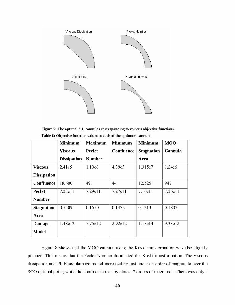
Figure 7: The optimal 2-D cannulas corresponding to various objective functions.
Table 6: Objective function values in each of the optimum cannula.
Minimum
Viscous
Dissipation
Maximum
Peclet
Number
Minimum
Confluence
Minimum
Stagnation
Area
MOO
Cannula
Viscous
Dissipation
2.41e5 1.10e6 4.39e5 1.315e7 1.24e6
Confluence 18,600 491 44 12,525 947
Peclet
Number
7.23e11 7.29e11 7.27e11 7.16e11 7.26e11
Stagnation
Area
0.5509 0.1650 0.1472 0.1213 0.1805
Damage
Model
1.48e12 7.75e12 2.92e12 1.18e14 9.33e12
Figure 8 shows that the MOO cannula using the Koski transformation was also slightly
pinched. This means that the Peclet Number dominated the Koski transformation. The viscous
dissipation and PL blood damage model increased by just under an order of magnitude over the
SOO optimal point, while the confluence rose by almost 2 orders of magnitude. There was only a
40
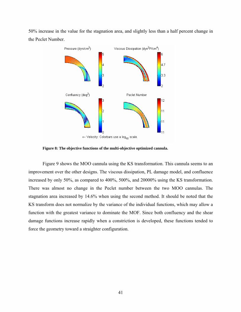
50% increase in the value for the stagnation area, and slightly less than a half percent change in
the Peclet Number.
Figure 8: The objective functions of the multi-objective optimized cannula.
Figure 9 shows the MOO cannula using the KS transformation. This cannula seems to an
improvement over the other designs. The viscous dissipation, PL damage model, and confluence
increased by only 50%, as compared to 400%, 500%, and 20000% using the KS transformation.
There was almost no change in the Peclet number between the two MOO cannulas. The
stagnation area increased by 14.6% when using the second method. It should be noted that the
KS transform does not normalize by the variance of the individual functions, which may allow a
function with the greatest variance to dominate the MOF. Since both confluency and the shear
damage functions increase rapidly when a constriction is developed, these functions tended to
force the geometry toward a straighter configuration.
41

Figure 9: Second set of multi-objective optimized (MOO) cannulae.
42

4.0 DISCUSSION AND CONLUSIONS
There are numerous possible choices for objective functions that represent blood damage.
Viscous dissipation, confluency, stagnation area, and Peclet Number were all shown to have
great promise in observing blood damage in its various forms. They were selected above the rest
because they had better qualities than the other function. Viscous dissipation had a reasonable
resemblance to the power-law blood damage models for shear induced hemolysis and platelet
activation, but showed better mathematical behavior. Confluency, which is somewhat difficult to
define, was very effective at penalizing designs with recirculation regions. Recirculation is
typically linked with high shear rates and buildup of platelet agonist and coagulation factors.
Stagnation area is a distant second to confluency, if an unacceptable reference flow field cannot
be found. It has a decent variance over the design space, but cannot be used to penalize
recirculation zones that have high velocities. Peclet Number is a good index for representing the
clearance of agonists, coagulation factors, and active platelets. It suffers from a small variance in
the design space, but also serves to balance the behavior of viscous dissipation. All three
objective functions exhibited robust performance about their optimal points, and are therefore
good selections.
This study illustrates the crucial importance of multi-objective optimization for designing
blood-wetted medical devices, because the mechanism for various forms of blood damage
compete with one another. For example, shear, which is a measure of hemolysis and platelet
activation, competes with convection, which is a measure of agonist build up, platelet adhesion,
and the build up of coagulation factors. Unfortunately, multi-objective optimization is still in its
infancy and an ideal approach has not been fully developed. Currently, two popular and
systematic methods were used based on normalizing the objective functions and do show
reasonable results.
43

4.1 QUALITATIVE ANALYSIS OF OBJECTIVE FUNCTIONS
The qualitative analysis gave great insight into the ability of several functions to evaluate blood
damage. Several objective functions showed very similar patterns in the flow field, which would
indicate that they are correlated with one another. The total area of the design was shown to
contribute to the optimal point. This type of analysis extends beyond optimization and is suitable
for analyzing CFD results in general. This allows for different design options or devices to be
compared, using the user preferred CFD package.
This analysis also gives preliminary guidance into which objectives are appropriate for
optimization. It is obvious that confluency is the only objective function that properly defines
recirculation regions in an Eulerian frame of reference. The Peclet Number also provides a good
indicator for the clearance in a device. The various functions that relate to shear induced
hemolysis and platelet activation show similar features. This tends to indicate that they are
interchangeable and that there is no preference in using one over the other, but further analysis is
necessary in order to show that this correlation exists.
4.2 QUANTITATIVE ANALYSIS OF OBJECTIVE FUNCTIONS
A more mathematical analysis of the objective function validated some of the results from the
qualitative analysis, but also gave more insight into the behavior of the objective functions. The
blood damage models have been reduced to viscous dissipation, or elongation in the principal
frame, the confluency or stagnation area, and Peclet Number. These functions are not correlated
with each other and provide a good basis for multi-objective optimization.
Several objective functions were eliminated out of mathematical preference, first through
logical deduction and secondly by examining their Hessian matrix. The first function that was
eliminated was vorticity since it only correlates to shear stress (a known cause of hemolysis) but
does not have its own mechanism for destroying blood cells. Unlike viscous dissipation and
shear stress, which are linked to blood damage through mechanistic means, flows with high
shear, especially turbulent flow, generally have high vorticity, but vorticity can occur where
there is no shear. Blackshear suggests that turbulent eddies on the scale of the RBC cause
44
hemolysis, but the means of damage is not clear. The second problem with this reasoning is that
our current modes of simulation cannot simulate eddies of this size. But, consider solid body
rotation of a fluid with the same density of a red blood cell. This is a flow that has vorticity
(twice the rotational rate) but no shear stress. Logically, one would expect that there would be no
hemolysis in the solid body rotation since there is no deformation of the cells. The work of
Sutera et al. (33) seems to support this hypothesis. They measured the effect of turbulence on
hemolysis, and showed that free turbulence did not raise the level of hemolysis. The turbulence
does increase hemolysis when in the presence of a wall because it increases the shear stress at the
wall. Currently we are discussing several experiments in order to investigate this hypothesis, but
for now it will be dropped until further study can be made.
The second function that should be dropped is the elongation. Elongation is commonly
used in chemical engineering for studying polymer flows. As mention above, it is the RMS value
of the normal components of the strain rate tensor, D. There is a debate as to what frame of
reference should be used to determine the elongation of a cell. Four frames are important to
consider. The first is the Eulerian fixed frame, which simplifies the problem considerable since
no transformations are necessary to calculate the function. The second frame is the local flow
frame, where the elongation is calculated along the streamline. This is how polymers usually
align themselves in the flow field. Thirdly, there is the principal frame where the elongation
should be at its maximum. The forth is based off of experimental results.
Normally, we would expect the greatest deformation in the principal axis, but this is not
what is seen experimentally. For Couette flow, the principal axis is aligned at 45o but
experimental results show that the red blood cells align at approximately 20o with some variance
due to flow and hematocrit. This would indicate that the frame should be rotated 20o for Couette
flow, but it the angle of alignment is different for various flows. There is thus a large uncertainty
as to the frame in which elongation should be calculated. In the principal frame elongation
becomes the strain rate, meaning that ε2 is proportional to viscous dissipation. All the analysis for
viscous dissipation would then hold for principal elongation.
The second variations of select objective functions were evaluated for positive
definiteness in order to further reduce the number of objective functions. Normally, the second
variation would require the solution of the sensitivity of the PDE to the design parameter, but
45
this value is independent of the objective functions, so we will only worry about the behavior of
the objective functions themselves.
The convergence of an objective function is directly tied to its Hessian matrix. If the
matrix is positive definite, then the convergence to a minima is guaranteed and should be
relatively fast. If the matrix is not positive definite, then the optimization routine can be attracted
to a saddle point or a maximum. Convergence for functions that do not have positive definite
Hessians depends on the nearness of the guess to the initial point. The Hessian is related to the
second variation of the objective function found using calculus of variations. Variations were
calculated for viscous dissipation, the power-law blood damage models, residence time, and
Peclet Number (Table 7). The symbol “^” implies the first variation, while the symbol “~”
implies the second variation of the function. The second variation of the residence time and that
of the power-law damage functions have negative components, which indicate that the Hessian
may not be positive definite at all points. The second variations of viscous dissipation and the
Peclet Number are always positive definite which make them suitable for optimization.
46

Table 7: First and second variations of selected objective functions.
Function Variation
Order
Variational Form
Viscous
Dissipation
1st ( )∫Ω
Ω++++ dvvvuvuuu yyxyxyxx ˆ2)ˆˆ)((ˆ22μ
2nd ( )∫Ω
Ω++++ dvvvuvuuu yyxyxyxx ˆ~2)ˆˆ)(~~(ˆ~22μ
PL Blood
Damage
Model
1st
( )∫Ω
Ω⎟⎟⎠
⎞⎜⎜⎝
⎛+− dvvuu
UC
UC VDVD ˆˆˆ
3
μμ
2nd
( )
( )( )
( )∫
∫
∫
Ω
Ω
Ω
Ω⎟⎟⎠
⎞⎜⎜⎝
⎛+−
Ω⎟⎠⎞
⎜⎝⎛ +++
Ω⎟⎟⎠
⎞⎜⎜⎝
⎛+−
dvvuuUC
dvvuuvvuuUC
dvvuuUC
UC
VD
VD
VDVD
ˆ~ˆ~ˆ
ˆ~ˆˆ2
3
ˆˆˆ~
3
5
3
μ
μ
μμ
Residence
Time
1st
∫Ω
Ω⎟⎠⎞
⎜⎝⎛ +
− dU
vvuu3
ˆˆ
2nd
( )∫Ω
Ω⎟⎠⎞
⎜⎝⎛ +
+−
+− dvvuu
Uvvuu
Uvvuu ~~ˆˆ
23ˆ~ˆ~
53
Peclet
Number
1st
∫Ω
Ω⎟⎟⎠
⎞⎜⎜⎝
⎛ + dD
dvvuu2
2)ˆˆ(2
2nd
∫Ω
Ω⎟⎟⎠
⎞⎜⎜⎝
⎛ + dD
dvvuu2
2)ˆ~ˆ~(2
47
4.3 OPTIMIZATION OF A 2-D CANNULA
There were several interesting results from this study. The first is that the power-law objective
function did indeed behave poorly, just as predicted by the mathematical analysis.
Approximation methods, like the Picard Method, must be used if the power-law models are to be
implemented. This means that the user must use more advanced optimization techniques, and
cannot use the common canned methods. The other option is to use viscous dissipation. The two
did reach the same optimal point, and no special method would be required for the convergence.
The optimal shapes for these types of functions were used in section 4, and shows that the
damage function is dominated by the shear stress. Since the flow is low enough, the stress caused
by the recirculation zone is not large enough to impact the value of the objective function. The
cannula increased its size in order to reduce the flow rate and the resulting stresses, until it
reached the pre-described limits of the shape (6.2). It is possible that there is a point, where flow
rate decreased enough to where the velocity term would dominate, but the constraints prevented
this.
The Peclet Number was optimized and the cannula appeared to have a slight constriction
in its side. The size of the cannula decreases in order to increase the flow speed through the
cannula. This makes sense, since the Peclet number is the balance of convection to diffusion. The
cannula must increase the velocity, since the diffusion term is constant. The value seems to reach
a balance at the point where flow would start to separate and cause a low velocity recirculation
region at the distal end.
The cannula generated by the confluence objective function was nearly circular, and if
weighted Bezier curves had been used to describe the geometry, it would probably be completely
circular. This again makes sense because the desired flow angle was selected to a circular path.
This however implies that the use of the confluency objective is fairly limited to the user’s a-
priori definition of the desired flow path. In some circumstances this would be desirable;
however for complex flow, it would be more advantageous to use the Stokes flow solution (low
Reynolds Number) to prescribe the desired path. Stokes flows are dominated by viscosity, as
opposed to momentum, and will typically not exhibit recirculation zones. Any recirculation
zones that appear at higher Reynolds numbers will show a significant deviation from the Stokes
flow. This method also solves the problem of more complex geometries.
48

This thesis has lead to a novel and innovative design of ventricular cannula that shows
numerical improvements over the previous design. The cannula has a larger upper portion, which
tapers down as it approaches the device. This reduces shear, since the initial flow is lower. It also
reduces the “sloshing” of blood toward the outer portion of the pipe. This phenomenon is
momentum related, and is reduced by having a lower momentum going into the turn. This also
decreases the high shear stress that forms when the fluid from the central core contacts the outer
wall. Finally, this design reduces the strength of the Dean vortices, which improves the blood
damage as well as the efficiency of the VAD to which it is connected. The new cannula then
tapers, causing the flow to accelerate. This increases the shear rate, but also increases the
convection of the undesirable chemicals and platelets. Another important result is that the
velocity profile is more uniform than the previous one. This also helps to improve the efficiency
of the VAD.
49

5.0 FUTURE WORK
This thesis had two goals. The first was to advance the understanding of current methods for
relating CFD results to blood damage. The objective functions that were chosen represent either
common methods of determining blood damage or other functions that seem to fit well with
concepts of blood damage. Although this list was comprehensive there are certainly other
methods that could be examined. It is also desirable to combine CFD with other simulation
techniques, such as the convection-diffusion (C-D) equation, which could be used to explicitly
compute clearance (wash out.) Even more complex than the C-D equation are various models of
platelet aggregation. Another area of future work also includes modeling actual blood cell
rupture. Finally, the power-law blood damage models can be evaluated in a Lagrangian frame of
reference. All three of these areas require more work in order to have a better understanding of
blood damage on both a macroscopic and microscopic level.
Besides examining new methods for describing blood damage, the current models were
only examined in a simple 2-D flow. More work should be done in order to compare these
objectives in more complex flows, for example through a blade path of a ventricular assist
device, or in 3D flow cases. For this thesis, it was assumed that the results would be the same as
in the 3D case. Verification would still be necessary to prove this hypothesis. Other variations
that must be analyzed involve other flow equations, such as turbulent flow, non-Newtonian flow,
and visco-elastic flows.
Future continuation of this research should also consider the use of more robust methods
of optimization. The description of the geometry, for example should be refined to minimize the
curvature and thus be less sensitive to errors in manufacturing or other factors that were not
taken into account in simulation or optimization routine. These factors can include changes in
viscosity or other alteration in the blood flow, defects in cannula, and changes caused by
implantation.
50

The second goal of this thesis was to improve the design of a specific flow path,
representative of a ventricular cannula. The new cannula resulting from this optimization
exercise would benefit from experimental validation for its superiority to be definitively
convincing. This will help verify that the selected objective functions are acceptable, and more
importantly demonstrate that there is significant room for improvement in the design of cannula.
Future extension of this research should also consider the design over a range of
operating conditions. Flow in the cardiovascular system is not constant and should be taken into
account in the optimization routine. Several methods could be used, including pulsatile flow and
optimization in unsteady flow. This is very difficult and computationally expensive, and still
assumes a flow regime that might not be ideal. Another method that could possibly help deal
with this is to run multi-objective optimization of a range of flow conditions with, but weight the
desired flow regime higher than the outliers. VADs sometime allow for the heart of the patient to
recover, in which case the patient is weaned off of the device. This means that the Cannula and
VADs must be designed to operate at lower flow rates than normal to accommodate weaning of
patients. This can likewise be accommodated with a time varying flow that is either ramped up to
nominal or vice versa, or by using a weighted function over the flow regime.
Finally, the optimal design of the cannula tip is important. Carefully consideration must
be taken to account for the heart-cannula interaction. Thrombosis commonly occurs at the area
where the cannula is placed into the heart. Another challenge is that the blood can be damaged at
the entrance to the cannula, so hemolysis could potentially be decreased by shape optimization.
Also, the exact placement of the cannula within the ventricle is impossible since it is not possible
to see inside the ventricle during implantation and each heart is unique. Multi-objective
optimization could also be implemented to reduce the effects of less than ideal placement using
similar weighting methods as described above.
51
BIBLIOGRAPHY
1. Giersiepen M, Wurzinger LJ, Opitz R, Reul H. Estimation of shear stress-related blood damage in heart valve prostheses--in vitro comparison of 25 aortic valves. Int J Artif Organs 1990;13(5):300-6.
2. James NL, Wilkinson CM, Lingard NL, van der Meer AL, Woodard JC. Evaluation of hemolysis in the VentrAssist implantable rotary blood pump. Artif Organs 2003;27(1):108-13.
3. Grigioni M, Daniele C, Morbiducci U, D'Avenio G, Di Benedetto G, Barbaro V. The power-law mathematical model for blood damage prediction: analytical developments and physical inconsistencies. Artif Organs 2004;28(5):467-75.
4. Sorensen EN, Burgreen GW, Wagner WR, Antaki JF. Computational simulation of platelet deposition and activation: I. Model development and properties. Ann Biomed Eng 1999;27(4):436-48.
5. Sorensen EN, Burgreen GW, Wagner WR, Antaki JF. Computational simulation of platelet deposition and activation: II. Results for Poiseuille flow over collagen. Ann Biomed Eng 1999;27(4):449-58.
6. Ogino H, Klangsuk N, Jin W, Bowles CT, Yacoub MH. Influence of the compliance of the pump housing and cannulas of a paracorporeal pneumatic ventricular assist device on transient pressure characteristics. Artif Organs 1995;19(6):525-34.
7. Ogino K, Hisatome I, Kotake H, Furuse T, Mashiba H, Kuroda H, et al. A case of four coronary artery fistulae originating from three vessels associated with aneurysm. Eur Heart J 1987;8(11):1260-3.
8. Richenbacher WE, Marks JD. Cannula selection and cannulation techniques for nonpulsatile mechanical ventricular assistance. Artif Organs 1995;19(6):519-24.
9. Deleuze P, Okude J, Leandri J, Rey P, Loisance D. An original inflow cannula for paracorporeal assist devices. ASAIO Trans 1989;35(3):442-4.
10. Curtis AS. A Multiple Modality Study of the Hemodynamics of Left Ventricular Cannulation [Masters of Science in Biomedical Engineering]. Pittsburgh: University of Pittsburgh; 1998.
52

11. He B. Shape Optimization of Navier-Stokes Flow with Application to Design of Artificial Heart Components [Ph.D]. Pittsburgh: Carnegie Mellon University; 1996.
12. Antaki JF, Dennis TJ, Konishi H, Brown ME, Maher TR, Tomczak JP, et al. An improved left ventricular cannula for chronic dynamic blood pump support. Artif Organs 1995;19(7):671-5.
13. Hanson SR. Device Thrombosis and Thromboembolism. Cardiovasc. Pathol. 1993;2:157S-165S.
14. Guyton AC, Hall JE. Textbook of medical physiology. 10th ed. Philadelphia: Saunders; 2000.
15. Saladin KS. Anatomy & physiology: the unity of form and function. 2nd ed. Boston: McGraw-Hill; 2000.
16. Chien S, Usami S, Taylor HM, Lundberg JL, Gregersen MI. Effects of hematocrit and plasma proteins on human blood rheology at low shear rates. J Appl Physiol 1966;21(1):81-7.
17. Paut O, Bissonnette B. Effects of temperature and haematocrit on the relationships between blood flow velocity and blood flow in a vessel of fixed diameter. Br J Anaesth 2002;88(2):277-9.
18. Walburn FJ, Schneck DJ. A constitutive equation for whole human blood. Biorheology 1976;13(3):201-10.
19. Thurston GB. Viscoelasticity of human blood. Biophys J 1972;12(9):1205-17.
20. Deutsch S, Phillips WM. An interpretation of low strain rate blood viscosity measurements: a continuum approach. Biorheology 1976;13(5):297-307.
21. Sharp MK, Thurston GB, Moore JE, Jr. The effect of blood viscoelasticity on pulsatile flow in stationary and axially moving tubes. Biorheology 1996;33(3):185-208.
22. Mann DE, Tarbell JM. Flow of non-Newtonian blood analog fluids in rigid curved and straight artery models. Biorheology 1990;27(5):711-33.
23. Mann KA, Deutsch S, Tarbell JM, Geselowitz DB, Rosenberg G, Pierce WS. An experimental study of Newtonian and non-Newtonian flow dynamics in a ventricular assist device. J Biomech Eng 1987;109(2):139-47.
24. Mizuno T, Tsukiya T, Taenaka Y, Tatsumi E, Nishinaka T, Ohnishi H, et al. Ultrastructural alterations in red blood cell membranes exposed to shear stress. Asaio J 2002;48(6):668-70.
25. Blackshear PL, Jr., Dorman FD, Steinbach JH. Some Mechanical Effects That Influence Hemolysis. Trans Am Soc Artif Intern Organs 1965;11:112-7.
53

26. Blackshear PL, Jr., Dorman FD, Steinbach JH, Maybach EJ, Singh A, Collingham RE. Shear, wall interaction and hemolysis. Trans Am Soc Artif Intern Organs 1966;12:113 20.
27. Bernstein EF, Blackshear PL, Jr., Keller KH. Factors influencing erythrocyte destruction in artificial organs. Am J Surg 1967;114(1):126-38.
28. Blackshear PL, Jr., Forstrom RJ, Dorman FD, Voss GO. Effect of flow on cells near walls. Fed Proc 1971;30(5):1600-11.
29. Reul H, Talukder N, Muller EW. Fluid mechanics of the natural mitral valve. J Biomech 1981;14(5):361-72.
30. Wurzinger LJ, Opitz, R., Eckstein, H. Mechanical Blood Trauma. Angeilogie 1986;38(3):81-97.
31. Umezu M, Fujimasu, H., Yamada, T., Fijimoto, T., Ranakawake, M., Nogawa, A., and Kijima T. Fluid Dynamic Investigation of Mechanical Blood Hemolysis. Heart Replacement: The 5th International Symposium on Artificial Heart and Assist Devices 1995;5:327-335.
32. Kingsbury C, Kafesjian R, Guo G, Adlparvar P, Unger J, Quijano RC, et al. Cavitation threshold with respect to dP/dt: evaluation in 29 mm bileaflet, pyrolitic carbon heart valves. Int J Artif Organs 1993;16(7):515-20.
33. Sutera SP, Croce PA, Mehrjardi M. Hemolysis and subhemolytic alterations of human RBC induced by turbulent shear flow. Trans Am Soc Artif Intern Organs 1972;18(0):335-41, 347.
34. Sutera SP, Mehrjardi MH. Deformation and fragmentation of human red blood cells in turbulent shear flow. Biophys J 1975;15(1):1-10.
35. Jaenike JR. The renal lesion associated with hemoglobinemia. I. Its production and functional evolution in the rat. J Exp Med 1966;123(3):523-35.
36. Jaenike JR, Schneeberger EE. The renal lesion associated with hemoglobinemia. II. Its structural characteristics in the rat. J Exp Med 1966;123(3):537-45.
37. Jaenike JR. The renal lesion associated with hemoglobinemia: a study of the pathogenesis of the excretory defect in the rat. J Clin Invest 1967;46(3):378-87.
38. Abrams C, and Lawrence, F.B. Platelet Signal Transduction. In: Coleman RW, Hirsh, J., Marder, V.J., Clowes, A.W., and George, J.N., editor. Hemostasis and Thrombosis: Basic Principles & Clinical Practice. 4th ed: Lippincott, Williams, and Wilkins; 2001. p. 541-559.
39. Tandon P, Diamond SL. Hydrodynamic effects and receptor interactions of platelets and their aggregates in linear shear flow. Biophys J 1997;73(5):2819-35.
54
40. Hanson SR, and Harker, L.A. Blood Coagulation and Blood-Material Interactions. Biomaterials Science 1996:193-198.
41. Mushahwar SS, Pyatt JR, Lowe R, Morrison WL, Perry RA, Ramsdale DR. Clinical outcomes of long coronary stents: a single-center experience. Int J Cardiovasc Intervent 2001;4(1):29-33.
42. Manolis AS, Chiladakis J, Hahalis G, Agelopoulos G. Initial experience with a newer generation coronary stent. J Invasive Cardiol 2001;13(3):217-22.
43. Holmes DR, Jr. In-stent restenosis. Rev Cardiovasc Med 2001;2(3):115-9.
44. Chuter TA. Stent-graft design: the good, the bad and the ugly. Cardiovasc Surg 2002;10(1):7-13.
45. Keiser JA, Uprichard AC. Restenosis: is there a pharmacologic fix in the pipeline? Adv Pharmacol 1997;39:313-51.
46. Sigwart U. Coronary stents. Z Kardiol 1995;84 Suppl 2:65-77.
47. Klugherz BD, Herrmann HC. Mechanical Prosthetic Valve Thrombosis: Case Report and Review of the Literature. J Thromb Thrombolysis 1998;6(3):253-259.
48. Vongpatanasin W, Hillis LD, Lange RA. Prosthetic heart valves. N Engl J Med 1996;335(6):407-16.
49. Antunes MJ. Reoperations on cardiac valves. J Heart Valve Dis 1992;1(1):15-28.
50. Metzdorff MT, Grunkemeier GL, Pinson CW, Starr A. Thrombosis of mechanical cardiac valves: a qualitative comparison of the silastic ball valve and the tilting disc valve. J Am Coll Cardiol 1984;4(1):50-3.
51. Kloster FE. Diagnosis and management of complications of prosthetic heart valves. Am J Cardiol 1975;35(6):872-85.
52. Hylen JC. Mechanical malfunction and thrombosis of prosthetic heart valves. Am J Cardiol 1972;30(4):396-404.
53. Wagner WR, Schaub RD, Sorensen EN, Snyder TA, Wilhelm CR, Winowich S, et al. Blood biocompatibility analysis in the setting of ventricular assist devices. J Biomater Sci Polym Ed 2000;11(11):1239-59.
54. Kasirajan V, McCarthy PM, Hoercher KJ, Starling RC, Young JB, Banbury MK, et al. Clinical experience with long-term use of implantable left ventricular assist devices: indications, implantation, and outcomes. Semin Thorac Cardiovasc Surg 2000;12(3):229-37.
55. 1997;62 Suppl 1.
55
56. Schwab SJ. Assessing the adequacy of vascular access and its relationship to patient outcome. Am J Kidney Dis 1994;24(2):316-20.
57. Albers FJ. Causes of hemodialysis access failure. Adv Ren Replace Ther 1994;1(2):107-18.
58. Haimov M. Vascular access for hemodialysis. Surg Gynecol Obstet 1975;141(4):619-25.
59. Bordenave L, Remy-Zolghadri M, Fernandez P, Bareille R, Midy D. Clinical performance of vascular grafts lined with endothelial cells. Endothelium 1999;6(4):267-75.
60. Callow AD. Problems in the construction of a small diameter graft. Int Angiol 1988;7(3):246-53.
61. Ritter EF, Kim YB, Reischl HP, Serafin D, Rudner AM, Klitzman B. Heparin coating of vascular prostheses reduces thromboemboli. Surgery 1997;122(5):888-92.
62. Burkel WE. The challenge of small diameter vascular grafts. Med Prog Technol 1988;14(3-4):165-75.
63. Antaki JF, Ghattas O, Burgreen GW, He B. Computational flow optimization of rotary blood pump components. Artif Organs 1995;19(7):608-15.
64. Jones SA. A relationship between Reynolds stresses and viscous dissipation: implications to red cell damage. Ann Biomed Eng 1995;23(1):21-8.
65. Sutera SP. Flow-induced trauma to blood cells. Circ Res 1977;41(1):2-8.
66. Yeleswarapu KK, Antaki JF, Kameneva MV, Rajagopal KR. A mathematical model for shear-induced hemolysis. Artif Organs 1995;19(7):576-82.
67. Mitamura Y, Nakamura, H., and Sekine, K. Prediction of Hemolysis in Rotary Blood Pumps with Computational Fluid Dynamics Analysis. J. Congestive Heart Failure Circulatory Support 2000;1(4):331-336.
68. Wootton DM, Ku DN. Fluid mechanics of vascular systems, diseases, and thrombosis. Annu Rev Biomed Eng 1999;1:299-329.
69. Jesty J, Yin W, Perrotta P, Bluestein D. Platelet activation in a circulating flow loop: combined effects of shear stress and exposure time. Platelets 2003;14(3):143-9.
70. Tambasco M, Steinman DA. On assessing the quality of particle tracking through computational fluid dynamic models. J Biomech Eng 2002;124(2):166-75.
71. Joseph D. Interrogation of Direct Numerical Simulation of Solid-Liquid Flow. Minneapolis: University of Minneapolis; 2002.
56

72. Ghattas O, and Malcevic, I. Dynamic-Mesh Finite Element Method for Lagrangian Computational Fluid Dynamics. Finite Elements in Analysis and Design 2002;38.
73. Cardoze D, Cunha, A., Miller, G., Phillips, T., and Walkington N. A Bezier Approach to Unstructured Moving Meshes. Proceedings of the 20th Symposium on Computation Geometry 2004.
74. Burgreen GW, Antaki JF, Wu J, le Blanc P, Butler KC. A computational and experimental comparison of two outlet stators for the Nimbus LVAD. Left ventricular assist device. Asaio J 1999;45(4):328-33.
75. Chaubal CV, and Leal, L.G. Smoothed Particle Hydrodynamic Techniques for the Solution of Kinetic Theory Problems: Part 2. The effect of flow perturbations on the simplle shear behaviot of LCPs. J. Non-Newtonian Fluid Mech. 1999;82:25-55.
76. Goldsmith HL, Karino T. Platelets in a region of disturbed flow. Trans Am Soc Artif Intern Organs 1977;23:632-8.
77. Karino T, Goldsmith HL. Aggregation of human platelets in an annular vortex distal to a tubular expansion. Microvasc Res 1979;17(3 Pt 1):217-37.
78. Karino T, Goldsmith HL. Disturbed flow in models of branching vessels. Trans Am Soc Artif Intern Organs 1980;26:500-6.
79. Burgreen GW, Antaki JF, Griffith BP. A design improvement strategy for axial blood pumps using computational fluid dynamics. Asaio J 1996;42(5):M354-60.
80. Osher S, Fedkiw RP. Level set methods and dynamic implicit surfaces. New York: Springer; 2003.
81. Fogelson AL. Continuum models of Platelet Aggregation: Formulation and Mechanical Properties. SIAM J. Appl. Math 1992;52:1089-1110.
82. Gunzburger MD. Finite element methods for viscous incompressible flows: a guide to theory, practice, and algorithms. Boston: Academic Press; 1989.
83. Johnson C. Numerical Solution of Partial Differential Equations by Finite Elements Method: Cambridge University Prss; 1990.
84. Hansbo P, and Szepessy, A. A Velocity-Pressure Streamline Diffusion Finite Element Method for the Incompressible Navier-Stokes Equations. Computational Methods in Applied Mechanics and Engineering 1990;84:175-192.
85. Hughes T, Franca, L., and Hulbert, G. A New Finite Element Formulation for Computational Fluid Dynamics: Viii the Galerkin/Least-Squares Method for Advection-Diffusion Equations. Computational Methods in Applied Mechanics and Engineering 1989;73:173-189.
57
86. Behr MaT, T. Finite Element Solution Strategies for Large-Scale Flow Simulations. Computational Methods in Applied Mechanics and Engineering 1994;112:3-24.
87. Hughes T, Liu, W., and Brooks, A. Finite Element Analysis of Incompressible Viscous Flows by the Penalty Function Formulation. Journal of Computional Physics 1979;30:1-60.
88. Codina R. An Iterative Penalty Method for the Finite Element Solution of Stationary Navier-Stokes Equations. Computational Methods in Applied Mechanics and Engineering 1993;110:237-262.
89. Mizukami A. Element-by-Element Penalty / Uzawa Formulation for Large Scale Flow Problems. Computational Methods in Applied Mechanics and Engineering 1994;112:283-289.
90. Fletcher R. Practical Methods of Optimization: John Wiley and Sons.; 1980.
91. Gill PE, Murray, W., and Wright, M.H. Practical Optimization. London: Academic Press; 1981.
92. Hoffman JD. Numerical methods for engineers and scientists. 2nd ed. New York: Marcel Dekker; 2001.
93. Broyden CG. The Convergence of a Class of Doupe-rank Minimization Algorithms. J. Inst. maths. Applics. 1970;6:76-90.
94. Fletcher R. A New Approach to Variable Metric Algorithms. Computer Journal 1970;13:317-322.
95. Goldfarb D. A Family of Variable Metric Updates Derived by Variational Means. Mathematics of Computing 1970;24:23-26.
96. Shanno DF. Conditioning of Quasi-Newton Methods for Function Minimization. Mathematics of Computing 1970;24(647-656).
97. Fletcher R, and Powell, M.J.D. A Rapidly Convergent Descent Method for Minimization. Computer Journal 1963;6:163-168.
98. Davidson WC. Variable Metric Method for Minimization. A.E.C. Research and Development Report 1959;ANL-5990.
99. Schittowski K. NLQPL: A FORTRAN-Subroutine Solving Constrained Nonlinear Programming Problems. Annals of Operations Research 1985;5:485-500.
100. Powell MJD. A Fast Algorithm for Nonlinearly Constrained Optimization Calculations. In: Watson GA, editor. Numerical Analysis: Springer Verlag; 1978.
58
101. Han SP. A Globally Convergent Method for Linear Programming. J. Optimization Theory and Applications 1977;22:297.
102. Biggs MC. Constrained Minimization Using Recursive Quadratic Programming. In: Dixon LCW, and Szergo, G.P., editor. Towards Global Optmization: North-Holland; 1975. p. 341-349.
103. Da Cunha NO, and Polak, E. Constrained Minimization Under Vector-valued Criteria in Finite Dimensional Spaces. j. Math. Anal. Appl. 1967;19:103-124.
104. Censor Y. Pareto Optimality in Multiobjective Problems. Appl. Math. Optimiz. 1977;4:41-59.
105. Marler RT, and Arora, J.S. Survey of Multi-Objective Optimization Methods for Engineering. Struct Multidisc Optim 2004;26:369-395.
106. Koski J, and Silvernnoinen, R. Norm Methods and Partial Weighting in Multicriterion Optimization of Structures. Int. J. Numer. Methods Eng. 1987;24:1101-1121.
107. Koski J. Multicriterion Optimization in Structural Design. In: Atrek E, Gallegher, R.H., Ragsdell, K.M., Zienkiewicz, O.C., editor. New Directions in Optimum Structural Design. New York: John Wiley and Sons; 1984. p. 483-503.
108. Kolesov VI, Levin AO, Vinogradov AG, Danilova LD. [on Changes of Morphological and Functional Properties of the Blood and Hemodynamics During the Use of the Niiekhaii (Aik-59) and Baliuzek's (Isl-2) Artificial Circulation Apparatus]. Grudn Khir 1963;49:34-40.
109. Smithwick W, 3rd, Kouchoukos NT, Karp RB, Pacifico AD, Kirklin JW. Late stenosis of Starr-Edwards cloth-covered prostheses. Ann Thorac Surg 1975;20(3):249-55.
110. Anzai N, Iriyama T, Yamada M, Ishihara S. Intravascular hemolysis with pulmonic stenosis. Occurrence after correction of subpulmonary ventricular septal defect. Chest 1977;71(4):561.
111. Solanki DL, Sheikh MU. Fragmentation hemolysis in idiopathic hypertrophic subaortic stenosis. South Med J 1978;71(5):599-601.
59