Helioseismology

Laurent Gizon (lecturer)

Winter 2006/07 Course:5-16 February 2007

These are the lecture notes of a lecture given at the University of Gottingen and the MaxPlanck Institute for Solar System Research in Katlenburg-Lindau, respectively.The lecture was given by Dr. Laurent Gizon. These notes are summaries of the lecture,written down by students which were attending the lecture.The authors of each single chapter are in detail:

Chapter 2: Nazaret Bello Gonzalez, Julian Blanco Rodrıguez, Bruno Sanchez-Andrade Nuno, Thorsten Stahn, Danica Tothova

Chapter 3: Nazaret Bello Gonzalez, Julian Blanco Rodrıguez, Nilda Oklay, BrunoSanchez-Andrade Nuno, Thorsten Stahn, Danica Tothova, Esa Villenius,Jean-Baptiste Vincent

Chapter 4: Khalil Daiffallah, Kristian Hallgren, Emre Isik, Christian Koch, CorneliaMartinecz, Martin Meling, Silvia Protopapa, Pedro Russo, Jean Santos,Clementina Sasso, Sofi Spjuth, Julia Thalmann, Cecilia Tubiana, LotfiYelles

Chapter 5: Christian Koch

For further information, additional material, and useful links you may visit the followingwebsite: Helioseismology lecture

Contents

1 Survey of helioseismology and asteroseismology aims and results 2

2 Observed properties of stars 32.1 Isolated spherical stars . . . . . . . . . . . . . . . . . . . . . . . 32.2 Factors influencing observed properties of stars . . . . . . . . . . 32.3 Radiation from the star . . . . . . . . . . . . . . . . . . . . . . . 32.4 Mass Ms . . . . . . . . . . . . . . . . . . . . . . . . . . . . . . . 52.5 Stellar radius . . . . . . . . . . . . . . . . . . . . . . . . . . . . 5

3 Dynamical structure of stars 63.1 Hydrostatic equilibrium . . . . . . . . . . . . . . . . . . . . . . . 63.2 Validity of this approximation . . . . . . . . . . . . . . . . . . . 63.3 Equation of state . . . . . . . . . . . . . . . . . . . . . . . . . . 83.4 The virial Theorem . . . . . . . . . . . . . . . . . . . . . . . . . 83.5 Another derivation . . . . . . . . . . . . . . . . . . . . . . . . . 10

4 Linear Stellar Oscillations 144.1 Eulerian and Lagrangian perturbations . . . . . . . . . . . . . . . 14

4.1.1 Equations of the fluid . . . . . . . . . . . . . . . . . . . 154.1.2 Equations of linear oscillations : . . . . . . . . . . . . . . 15

4.2 Eigenvalue problem of linear oscillations . . . . . . . . . . . . . . 164.2.1 Eigenvalue problem . . . . . . . . . . . . . . . . . . . . 164.2.2 Boundary conditions . . . . . . . . . . . . . . . . . . . . 164.2.3 Orthogonality of eigenfunctions . . . . . . . . . . . . . . 184.2.4 Variational principle . . . . . . . . . . . . . . . . . . . . 19

4.3 Linear perturbation theory . . . . . . . . . . . . . . . . . . . . . 204.4 Asymptotic description of p-mode frequencies . . . . . . . . . . . 20

4.4.1 Duvall’s law . . . . . . . . . . . . . . . . . . . . . . . . 204.4.2 More rigorous analysis . . . . . . . . . . . . . . . . . . . 21

5 Inversion of p-mode frequencies 245.1 Abel inversion of Duvall’s law . . . . . . . . . . . . . . . . . . . 245.2 Regularized least-squares & optimally localized averages inversions 26

1

Chapter 1

Short survey of helioseismology andasteroseismology aims and results

Here is a list of some topics in solar (and stellar) physics which may be investi-gated with the tool of helioseismology:

• What is the mechanism of the solar cycle?

• Dynamo theory: How does motions in the sun generate the magnetic fieldof the sun

• Large scale flows (e.g. meridional flows), convective flows

• The internal magnetic field of the sun

• Active regions: (detailed) structure, emergence, evolution

• Space weather

• Basic physics: neutrinos, G, micro physics (equation of state), etc.

For a more detailed overview about the aims of helio- and asteroseimologyas well as some of its results including some nice pictures and movies, have alook at the Power Point Presentation “Introduction” on the website of the lecture(http://www.mps.mpg.de/projects/seismo/Helioseismology.html).

2

Chapter 2

Observed properties of stars

2.1 Isolated spherical starsIn this section we assume an isolated, non magnetic, non rotating star. In thatcase it has a perfect spherical shape. If this star has a companion, forming abinary system, or any other massive body around, this could create deformations,and tidal forces, which we won’t take into consideration. We will also assumethat there is no interstellar medium in the surroundings, so that our line of sightis unperturbed. The assumption of neglecting rotation and magnetic fiels meansneglecting flattening of the polar regions due to the centrifugal forces, and stressesinside the star due to magnetic fields.

2.2 Factors influencing observed properties of starsMany characteristic properties of a star (such as structure, evolution and lifetime)are determined by its initial conditions, that is basically its initial mass, Ms, andits initial chemical composition.During its evolution, a star passes significant changes in some of its properties(e.g. Radius, Luminosity, Temperature, rotational speed), so that the stellar agebecomes another important factor influencing the observed properties.Finally, what we observe from a star, will be influenced by the distance betweenthe star and the observer and the interstellar medium that may be block or emit insome spectral regions

2.3 Radiation from the starThe radiation which is emitted by a star can be analyzed quantitatively, as theintegrated flux over a given spectral region, or qualitatively studying the shape ofthe spectral lines.Since, usually, most of the light comes from the region where we almost have ther-modynamic equilibrium, the energy distribution of the star can be approximated

3

Figure 2.1: Black body spectra for different temperatures.

by a black body, which follows the Planck law:

Iν = Bν(Ts) =2hν3

c2

[exp

(hν

kBTs

)− 1

]−1

(2.1)

In the prior equation, h, c and kB denote, respectively, the Planck’s constant,the speed of light and the Boltzmann constant. By considering a star as a blackbody, one may describe the Intensity Iν of the emitted light of a star at a certainfrequency ν by a Planck function, Bν(Ts), which solely depends on the surfacetemperature Ts. Figure 2.1 shows Intensity spectra for black bodies with differenttemperatures.In reality, the black body spectrum of star is superimposed by spectral lines fromphotons with higher or lower energy than the ones of the black body backgroundapproximation. Those photons come from regions where we might not have suchequilibrium, or a different temperature, leading to abortions or emission lines.Those lines will be mostly seen as absorption lines, due to the temperature gradi-ent. They not only reveal the chemical composition of the star, but may also beused to measure stellar oscillations trough their periodic doppler shifts.

The Luminosity of a star is the total amount of energy radiated at any directionper unit time (measured in W or J/s) and it is given by

Ls = 4πR2sσT 4

s , (2.2)

4

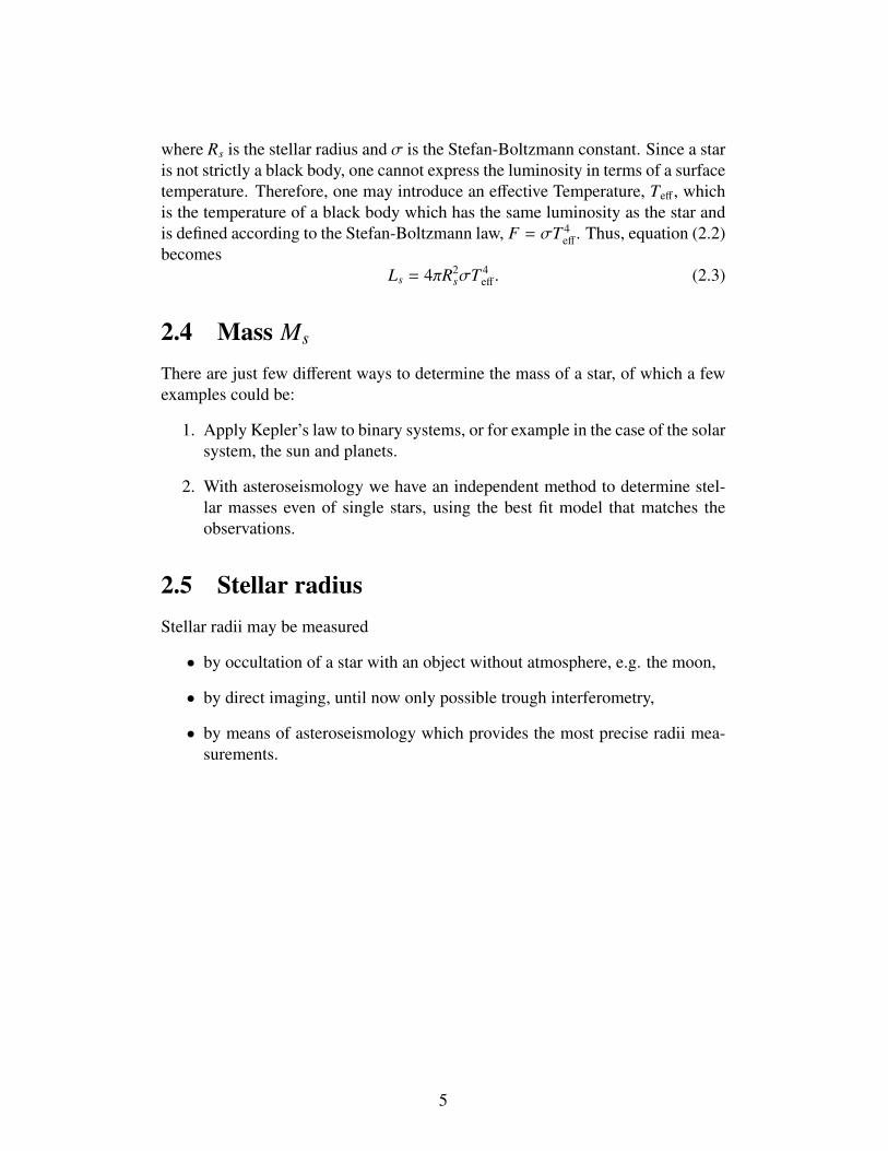
where Rs is the stellar radius and σ is the Stefan-Boltzmann constant. Since a staris not strictly a black body, one cannot express the luminosity in terms of a surfacetemperature. Therefore, one may introduce an effective Temperature, Teff, whichis the temperature of a black body which has the same luminosity as the star andis defined according to the Stefan-Boltzmann law, F = σT 4

eff. Thus, equation (2.2)

becomesLs = 4πR2

sσT 4eff. (2.3)

2.4 Mass Ms

There are just few different ways to determine the mass of a star, of which a fewexamples could be:

1. Apply Kepler’s law to binary systems, or for example in the case of the solarsystem, the sun and planets.

2. With asteroseismology we have an independent method to determine stel-lar masses even of single stars, using the best fit model that matches theobservations.

2.5 Stellar radiusStellar radii may be measured

• by occultation of a star with an object without atmosphere, e.g. the moon,

• by direct imaging, until now only possible trough interferometry,

• by means of asteroseismology which provides the most precise radii mea-surements.

5

Chapter 3

Dynamical structure of stars

3.1 Hydrostatic equilibriumConsider a thin spherical mass element with thickness δr and surface δs at a radiusr in the star. The gravitational force

FG =G[ρ(r)δsδr]M(r)

r2 (3.1)

acts on the mass element towards the stellar center. This gravitational force hasto be compensated by the difference of pressure force acting acting at radii r andr + δr:

[P(r + δr) − P(r)]δs = −FG (3.2)

Regarding that P(r + δr)− P(r) = ∂P∂r δr, equation (3.2) finally becomes the hydro-

static equation describing the solar structure:

∂P∂r

= −Gρ(r)M(r)

r2 (3.3)

Note that in the equation above, ρ(r) donotes the local density at radius r whileM(r) denotes an integral measure of the mass from the center up to the radius r.

3.2 Validity of this approximationIn order to proof the validity of the hydrostatic equilibrium, we may write theequation of motion (including only forces acting in radial direction) as

ρ

(∂vr

∂t+ vr∂rvr

)= −

∂P∂r

+ ρ∂φ

∂r, (3.4)

where the momentum of a mass element on left hand side of is generated by pres-sure forces and the gravitational force on right hand side.In general, the gravitational field inside the star can be described in terms of a

6

gravitational potential φwhich is the solution of a Poisson equation (here in spher-ical symmetry):

∇2φ =1r2∂r

(r2∂φ

∂r

)= −4πGρ (3.5)

Integration of equation (3.5) leads to an expression for ∂φ

∂r :∫ r

0∂r′

(r′2∂φ

∂r′

)dr′ = −

∫ r

04πGρr′2dr (3.6)

r2∂φ

∂r= −GM(r) (3.7)

∂φ

∂r=−GM(r)

r2 = g(r) (3.8)

Thus, equation (3.4) becomes

ρ

(∂vr

∂t+ vr∂rvr

)= −

∂P∂r

+ρGM(r)

r2 (3.9)

To proof the validity of the hydrostatic equilibrium, let us suppose

ρdvr

dt= −ε

ρGM(r)r2 , with: ε 1 (3.10)

As the most simple approximation, we can say the time for a substantial collapseof the star is given by the kinematic equation of the free fall in a gravitation field:

r = 12g(r)t2 = 1

2εGM(r)

r2 t2 (3.11)

⇒ t =

√1ε

2r3

GM(r) (3.12)

For the sun, we use r = R and M(r) = M(R) = M and obtain a collapse timeof t = 2 · 103 · ε−1/2sec. Assuming a minimal solar age of t > 4.4 · 109yr (accord-ing to the age of the oldest rocks on earth), one gets ε ∼ 10−28, showing that teassumption of hydrostatic equilibrium is very good.

Finally, we can summarise the first two equations describing the inner structure ofa star:

1. Mass conservation:dM(r)

dr= 4πρ(r)r2 (3.13)

2. Hydrostatic equilibrium:

∂P∂r

= −Gρ(r)M(r)

r2 (3.14)

7

3.3 Equation of stateWith an assumption of a star is an ideal gas:

P = Pgas + Pradiation (3.15)

Pgas = nkT =ρ(r)m

kT (3.16)

Mean molecular weight: m = µmH

Pgas = nkT =ρ(r)m

kT (3.17)

Pgas = ρ(r)µmH

kT(3.18)

(3.19)

Gas constant R = k/mH

Pgas = ρ(r)µ

RT Prad = 1/3aT 4 (3.20)

Equation of State:

P =ρRTµ

+13

aT 4 (3.21)

3.4 The virial Theorem

−Ω = 3∫ V

0PdV (3.22)

Ω is the negative gravitational energy of the star; V volume of a sphere ofradius r

3∫ V

0PdV = 3[PV]s

c − 3∫ s

cVdP (3.23)

= −3∫ s

cVdP (3.24)

= 4π∫ s

c

GM(r)r3ρ(r)r2 dr (3.25)

3∫ s

cPdV =

∫ s

c

GM(r)r

dM (3.26)

(3.27)

δΩ is the work required to bring δM from infinity to the sphere of radius r.

8

δΩ =

∫ r

∞

GM(r)δMx2 dx = −

GM(r)δMr

(3.28)

Ω = −

∫ s

c

GM(r)dMr

(3.29)

−Ω =

∫ s

c

GM(r)dMr

= 3∫ s

cPdV (3.30)

Theorem:

−Ω =

∫ s

c

GM(r)dMr

>

∫ s

c

GM(r)dMrs

(3.31)∫ s

c

GM(r)dMrs

=GM2

s

2rs(3.32)

−Ω >GM2

s

2rs(3.33)

(3.34)

Internal energy per unit volume is u = 1γ−1 P

γ is the ratio of specific heat: γ =cp

cv

P = (γ − 1)U (3.35)

−Ω = 3∫

(γ − 1)UdV = 3(γ − 1)U (3.36)

−Ω = 3(γ − 1)U (3.37)(3.38)

The total energy of a star would be

E = Ω + U = (4 − 3γ)U (3.39)

With this equation we can see where the star is stable or unstable:E < 0 stable→ γ > 4/3

E > 0 unstable→ γ < 4/3

For monoatomic gas, γ = 5/3

γ = 5/3→ Ω + U = −U (3.40)γ + 2U = 0 (3.41)

9

3.5 Another derivationWe can also derivate this theorem from Euler’s equation of fluid dynamics.

~r = −1ρ

−−−→gradP + ~Fgrav (3.42)

Then we multiply by ~r and integrate on the whole mass M∫M~r.~rdm = −

∫M

1ρ~r.−−−→gradPdm +

∫M~r. ~fgravdm (3.43)

We will now express separately the three components of this equation

(i)

∫M~r.~rdm =

∫M

(ddt

(~r.~r) − ~r2)

dm

=

∫M

(12

d2

dt2~r2 − ~r2

)dm

Here one can recognize the formulas of kinetic energy and momentum of in-ertia defined by

I =

∫M

r2dm

KE =12

∫M

r2dm

Finally, ∫M~r.~rdm =

12

d2Idt2 − 2KE (3.44)

(ii)

∫M

1ρ~r.−−−→gradPdm =

∫V~r.−−−→gradPdV

=

∫V

div(~rP)dV −∫

VPdiv(~r)dV

=

∫V

div(~rP)dV − 3∫

VPdV

=

∫S

P~rdS − 3∫

VPdV

We assume P = 0 at the surface of the star, so finally

10

∫M

1ρ~r.−−−→gradPdm = −3

∫V

PdV (3.45)

(iii) ∫M~r. ~fgravdm = Ω = Potential Energy of Gravitation (3.46)

At the end, we can now use 3.44, 3.45, 3.46 in 3.43, which brings us to anotherexpression of the virial theorem.

12

d2Idt2 − 2KE = 3

∫V

PdV + Ω (3.47)

12

I = 2KE + 3 (3γ − 1) U + Ω (3.48)

The gravitational energy of an isolated star is

−Ω =

∫GM (r)

rdM. (3.49)

If the structure of the star is homologous, fixed functions M(

rrs

)and ρ

(rrs

)can be

applied. In other words, the functional form remains the same when the size of astar is scaled. Making the following change of variables

M (r) = Ms f1

(rrs

)(3.50)

dMdr

dr = dM =Ms

rsf ′1

(rrs

)dr (3.51)

gives

−Ω =GM2

s

rsq, (3.52)

where q is the constant number

q =

∫ 1

0

f1 (x) f ′1 (x)x

dx. (3.53)

Now

I =

∫star

r2dM (3.54)

I = sMsr2s , (3.55)

11

where s is a constant.

rs = r0 + ε∆r (t) (3.56)

12

I = (3γ − 1) E + (4 − 3γ) Ω (3.57)

For a static case, when a star is in equilibrium, this becomes

0 = (3γ − 1) E + (4 − 3γ) Ω0. (3.58)

12

I =12

sMs∂2t (r0 + ε∆r)2 (3.59)

=12

sMs∂t

[(r0 + ε∆r) 2ε∆r

](3.60)

=12

sMs2r0ε∆r (3.61)

(3.62)

Ω = −qGM2

s

rs(3.63)

= −qGM2

s

r0

(1 + ε

∆rr0

)−1

(3.64)

= Ω0 + qGM2

s

r20

∆rε (3.65)

= Ω0

(1 − ε

∆rr0

)(3.66)

⇒ sMr0ε∆r = (3γ − 4) Ω0 + (4 − 3γ) Ω0

(1 − ε

∆rr0

)(3.67)

sMsr0∆r = − (4 − 3γ) Ω0∆rr0

(3.68)

Case γ > 43 , stable oscillations

∆r = C∆r, (3.69)

where C > 0 is a constant:

C = −Ω0 (4 − 3γ)

sr20 Ms

. (3.70)

Case γ < 43

C = −Ω0 (4 − 3γ)

Iq. (3.71)

12

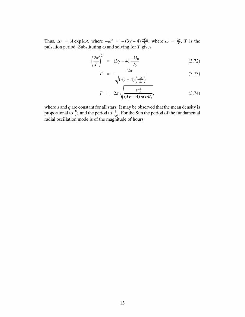
Thus, ∆r = A exp iωt, where −ω2 = − (3γ − 4) −Ω0I0

, where ω = 2πT , T is the

pulsation period. Substituting ω and solving for T gives(2πT

)2

= (3γ − 4)−Ω0

I0(3.72)

T =2π√

(3γ − 4)(−Ω0

I0

) (3.73)

T = 2π

√sr3

s

(3γ − 4) qGMs, (3.74)

where s and q are constant for all stars. It may be observed that the mean density isproportional to Ms

r3s

and the period to 1√ρ. For the Sun the period of the fundamental

radial oscillation mode is of the magnitude of hours.

13

Chapter 4

Linear Stellar Oscillations

4.1 Eulerian and Lagrangian perturbationsThe choice of independant variables differentiates the Eulerian and Lagrangianfluid descriptions. The position vector r and time t are the independent variables inan Eulerian fluid and any perturbation of the quantity Q is writen as Q′ = Q′(r, t) .This description is completly general since we suppose that the value of a variableat any point is uncorrelated with the value at a neighboring point. In contraste, theLagrangian description divides a fluid into tiny parcels. The independent variablesare the time t and the displacement vector ξ = r − r0 which are associated withparcels fluid, not points in space. The Lagrangian perturbation is denoted δQ(ξ, t).In terms of time derivatives in the case of Eulerian description, we write:

∂/∂t ≡ (∂/∂t)r (4.1)

derivative at fixed r.

In the case of Lagrangian description, we can write :

D0/Dt = (∂/∂t)r + (v0 · ∇) (4.2)

derivative at fixed r0 and comoving with to the backround flow v0.

Velocity perturbation:The displacement vector is defined as ξ = r − r0. The first order Lagrangian

variation of the vector v can writen as :

δv = v(r + ξ, t) − v0(r, t) = v(r, t) + (ξ · ∇)v − v0(r, t) (4.3)

we have also v(r, t) = v0(r, t)+v′(r, t) where v′(r, t) is the Eulerien perturbationof the velocity. The equation 4.3 become :

δv = v′(r, t) + (ξ · ∇)v0 (4.4)

14

From the definition of ξ we have also:

δv =D0ξ

Dt=∂ξ

∂t+ (v0 · ∇)ξ (4.5)

then we obtain :

v′ = δv − (ξ · ∇)v0 =D0ξ

Dt− (ξ · ∇)v0 (4.6)

4.1.1 Equations of the fluidMass conservation equation:

∂ρ

∂t+ ∇ · (ρv) = 0 (4.7)

Momentum equation:

ρDtv = −∇p − ρ∇φ (4.8)

where φ is the gravitational potentialPoisson equation:

4φ = 4πGρ (4.9)

where G is the constant of gravityEnergy equation:

ρT DtS = ρε − ∇ · F (4.10)

where S is the specific entropy, ρε is the internal energy density, F is theenergy flux and T is the temperature.

4.1.2 Equations of linear oscillations :At the equilibrium state, we have ∂t = 0 and the partial derivative in space vanishesalso, we have also v0 = 0 , we can write the fluid equations in this case as :

0 = −∇p0 − ρ0∇φ0 (4.11)

4φ0 = 4πGρ0 (4.12)

0 = ρ0ε0 − ∇ · F0 (4.13)

Perturbed state: Now we perturbe the pressure, the potential of the gravity,the density and the velocity with Eulerian perturbations, we replace all thesesquantities in the fluid equations. After the linearisation we obtain the equations oflinear oscillations:

15

ρ0∂2ξ

∂t2 = −∇p′ − ρ0∇φ′ − ρ′∇φ0 (4.14)

∂t(ρ′ + ∇ · (ρ0ξ)) = 0 (4.15)

4φ′ = 4πGρ′ (4.16)

ρ0T0∂t(δS ) = (ρ0ε)′ − ∇ · F′ (4.17)

4.2 Eigenvalue problem of linear oscillations

4.2.1 Eigenvalue problemThe basic equations of linear stellar oscillations (see previous section), describelinear adiabatic oscillations and can be solved for particular boundary conditions.Of course, these boundary conditions are satisfied for a set of special values of thefrequency ω – the eingenvalues.

4.2.2 Boundary conditionsSun center: As r → 0, c and ρ→ to a constant value, so one can write

g =GMr

r2 ≈4π3

r3Gρc

r2 → 0.

being ρc the value of the density at the Suns center. Furthermore, for theSchwarzschild discriminant A:

A→ 0 and L2l →

1r2 . (4.18)

After this assumptions, the simplified eigenvalue problem appears as

ddr

(r2ξr

)−

l(l + 1)ω2

(φ′ +

p′

ρ

)' 0, (4.19)

1ρ

dp′

dr− ω2ξr +

dφ′

dr' 0, (4.20)

ddr

(r2 dφ′

dr

)− l(l + 1)φ′ ' 0. (4.21)

16

Equating the different forms of the Poisson equation, one obtains

(r

ddr− l

) (r

ddr

+ l + 1)φ′ ' 0. (4.22)

This form of the Poisson equation now has two solutions, which are

rddr− l = 0 → φ′ ∼ rl, (4.23)

rddr

+ l + 1 = 0 → φ′ ∼ r−(l+1), (4.24)

where the latter is not a regular solution, since it goes to infinity for r → 0.Thus, we have (corresponding to 4.23)

rdφ′

dr= lφ′, (4.25)

and, combining 4.19, 4.20, and 4.23, one obtains for the radial componentof the displacement

ξr '1

ω2r2

(p′

ρ+ φ′

)for r→ 0. (4.26)

Solar surface: At the solar surface r → R the boundary conditions develop asfollows (Free surface boundary condition). From δp = 0:

p′ + ξ · ∇p = p′ − ρgξr = 0,p′ = ρgξr, (4.27)

As a second surface boundary condition, which only lasts in the Cowlingapproximation, we have ρ→ 0, resulting in

ξr =ω2R

gξh =

ω2R3

GMξh = (ωτdyn)2ξh, (4.28)

where τdyn denotes the dynamical time scale.

Our problem is still degenerate in m, since we assumed not to have effects ofthe magnetic field, rotation, and so on. This means, that if we evaluate the sameeigenfunctions for different m, we will obtain the same eigenvalues.

17

4.2.3 Orthogonality of eigenfunctionsNow, the eigenvalue problem can be written as

L[~ξ] = ω2ρ~ξ, (4.29)

which is the vector form of it and where L denotes the linear, second-orderdifferential operator. The solution of the problem is of the form

L[~ξnlm] = ω2nlm ρ ~ξnlm, (4.30)

i.e. that for each (l,m) one can find a number of solutions labeled with n. Then,n gives the number of modes of ξr in the radial direction. Now, one searchesfunctions which satisfy the boundary conditions at the center and the surface ofthe Sun, at the same time. One finds,

∫dV~ξ∗ · L(~ξ′) =∫

dV[− ξ∗ · ∇(ρc2∇ · ξ′) − ξ∗ · ∇(∇ρ · ξ′) +

∇p · ξ∗

ρ∇ · (ρξ′)

+ρξ∗ · ∇

[G

∫dV ′∇′[ρ(r′)ξ′(r′)]|r − r′|

] ]. (4.31)

This is then simplified by the ’integration by parts’, obtaining

∫dV

[ρc2(∇ · ξ∗)(∇ · ξ′) + (∇ · ξ∗)(∇p · ξ′)

]+

∫dV

[(∇p · ξ∗)(∇ · ξ′) +

(∇p · ξ∗)(∇ρ · ξ′)ρ

]− G

∫dV

∫dV ′∇[ρ(r)ξ∗(r)]∇′[ρ(r′)ξ′(r)]

|r − r′|. (4.32)

The main advantage of the form of 4.32 is that one can show now the invariantbehaviour of this equation. It also holds, if one swaps ξ and ξ′. Thus, it is

∫dVξ∗ · L(ξ′) =

∫dVξ′∗ · L(ξ) =

∫dV[L(ξ)]∗ · ξ′, (4.33)

then L is self-adjoint. Furthermore, one obtains for (n, l,m), after using 4.29the relation

ω2n′l′m′

∫dVξ∗nlm · ξn′l′m′ρ = ω∗2nlm

∫dVξ∗nlm · ξn′l′m′ρ. (4.34)

18

It can be shown that if (n, l,m) = (n′, l′,m′) then since the two integrals in 4.34are equal:

ω2n′l′m′ = ω∗2nlm, (4.35)

frequencies are real.This means, that unless some modes are degenerate, a given mode corresponds

to a given frequency. Last, the orthogonality of the eigenvectors ~ξnlm is given by

∫dVξnlm · ξn′l′m′ρ = δnn′δll′δmm′

∫dV ||ξnlm||

2ρ. (4.36)

4.2.4 Variational principleNote, that in the following the displacement vector will simply be denoted by writ-ing ξ instead of ~ξ. To obtain a very good estimate of frequencies when one is notable to solve the eigenvalue problem, one makes use of the variational principle,which can be written as

∫dVξ∗ · L(ξ) = ω2

∫dV ||ξ||2ρ. (4.37)

Effects of change of the displacement vector are represented by the substitu-tion ξ → ξ + ∆ξ. Now, one looks at the corresponding changes of the frequencyω2 → ω2 + (∆ω)2 and checks if 4.37 holds,

∫dV

[∆ξ∗ · L(ξ) + ξ∗ · L(∆ξ)

]=

(∆ω)2∫

dV ||ξ||2ρ + ω2∫

dV(ξ∗ · ∆ξ + ξ · ∆ξ∗)ρ, (4.38)

which represent the first-order changes that remain. Furthermore, since L isself-adjoint:

(∆ω)2∫

dV ||ξ||2ρ =∫dV

[∆ξ∗ · L(ξ) + (L(ξ∗))∗ · ∆ξ − ω2ρξ∗ · ∆ξ − ω2ρξ · ∆ξ∗

]=

2<∫

dV∆ξ∗ ·[L(ξ) − ω2ρξ

]. (4.39)

This implies, that (∆ω)2 → 0, i.e. ω2 is stationary with respect to a change ∆ξin ξ. In other words, this means that

19

(∆ω)2 = 0 (for an arbritrary ∆ξ) ⇐⇒ L(ξ) = ω2ρξ.

We show the implication⇐=.This forms the basis of the so-called ’Rayleigh-Ritz formula’ which is

ω2 =

∫dV(ξ + ∆ξ)∗ · L[ξ + ∆ξ]∫

dV ||ξ + ∆ξ||2ρ+ o(|∆ξ|2). (4.40)

So, the important thing concerning the variational principle is, that if onemakes a small variation inside the system one is still able to get a good approxi-mation of the frequency. In other words, if one assumes a small change ξ + ∆ξ inξ, one will still get the right ω.

4.3 Linear perturbation theory

4.4 Asymptotic description of p-mode frequencies

4.4.1 Duvall’s lawIf the wavelength is smaller than the variations in the local medium, the accoustic-wave dipersion relation takes in an important role:

ω2 = c2 | k |2= c2(k2r + k2

h) = c2(k2

r +l(l + 1)

r2

), (4.41)

where

kr =

[ω2

c2 −l(l + 1)

r2

]. (4.42)

kr has to fit the standing wave condition. Further a surface- induced phase shift αis introduced:∫ R

rt

krdr = (n + α)π, withc(rt)

rt=

ω

(l(l + 1))1/2 . (4.43)

This results in Duvall law (Duvall 1982; Nature 300, 242):

F(ω

L) =

∫ R

rt

(1 −

L2c2

ω2r2

)1/2 drc

=[n + α(ω)]π

ω,

L = l +12. (4.44)

c is a function of r. Fig. 4.1 shows the results of Duvall’s law for a frequencywhere α is taken as 1.5.

20

4.4.2 More rigorous analysisGough generalized the Duvall’s law. It is completely given in Deubner & Gough,1989 of an analysis by Lamb (1909). They assume:

• Cowling’s approximation,

• no derivatives of the gravitational acceleration, a quasiplane-parallel ap-proximation, and

• allow thermosdynamic variations, including γ1.

They define:X = c2ρ1/2∇ξ (4.45)

and retrieve:

d2Xdr2 +

Xc2

[S 2

l

(N2

ω2 − 1)

+ ω2 − ω2c

]= 0, (4.46)

where

H = −

(d(ln ρ)

dr

)−1

: density scale height,

ωc =c2

4H2

(1 − 2

dHdr

): accoustic cut-off frequency.

On transforming eq. (4.46) and taking a factor of ω2 from the brakets, the equationchanges to:

d2Xdr2 = −

Xc2ω2

[S 2

l

(N2 − ω2

)+ ω4 − ω2

cω2], (4.47)

the equation has 2 roots at (a2 −ω2) and (b2 −ω2) which can be retrieved throughstandard algebra. On introducing the roots in eq. (4.47) the equation can be writtento:

d2Xdr2 = −

Xc2ω2 (ω2 − ω2

+)(ω2 − ω2−), (4.48)

where ω+ is a modified Lamb frequency and ω− is a modified Bouyancy fre-quency. Fig. 4.2 shows a frequency plotted vs. the normalized radius of the Sun.The solid line shows the modified Lamb frequency for different degree l, whilethe broken line the modified Bouyancy frequency for different degrees l shows.Travelling waves have to have a frequency of ω ≥ ωc ' 5.3mHz. The conditionfor a standing wave can be written as:

ω

∫ r2

r1

[1 −

ω2c

ω2 −S 2

l

ω2

(1 −

N2

ω2

)]1/2drc' π(n − 1/2). (4.49)

For the standing wave the factor N2

ω2 can be neglected. Then ω2c

ω2 ' (n − 1/2).

21

Figure 4.1: Observed Duvall law where α is chosen to 1.5.

22

Figure 4.2: The frequency is plotted vs. the normalized Solar radius. The frequencies of ap-mode and the g-mode are inserted for comarison. Additionally the modified Lamb andBouyancy frequency are plotted for different degrees l.

23

Chapter 5

Inversion of p-mode frequencies

First Abel inversion will be shown for Duvall’s law. Afterwards two methods willbe described how to solve singularities in the inversion matrix.

5.1 Abel inversion of Duvall’s lawRemembering eq. (4.49) with a surface phase shift α Duvall’s law can be writtento: ∫ r2

r1

(1 −

L2c2

ω2r2

)1/2 drc

=[n + α]π

ω, (5.1)

whereL = l +

12. (5.2)

On introducing $ = ωL and a =

c(r)r , eq. (5.1) can be transformed to:

F($) =

∫ R

rt

(1 −

a2

$2

)1/2 drc. (5.3)

F are the observations and a(r) has to be found. After a change of variables,eq. (5.3) is:

F($) = −

∫ ω

as

(a−2 −$−2

)1/2 d(ln r)da

da, (5.4)

where:as = a(R⊙);

c(rt)rt

= $ = at; r = rt. (5.5)

On using (5.5) eq. (5.4) gets to:

dFd$

= −

∫ $

as

(a−2 −$−2

)1/2$−3 d(ln r)

dada. (5.6)

24

This results in and will be solved in the following:∫ a

as

($−2 − a−2

)1/2 dFd$

d$

= −

∫ a

as

∫ $

as

($−2 − a−2

)−1/2 (a−2 −$−2

)−1/2$−3 d(ln r)

dadad$

= −

∫ a

as

∫ a

a

($−2 − a−2

)−1/2 (a−2 −$−2

)−1/2$−3 d(ln r)

dad$da

= − −

∫ a

as

∫ π2

0

d(ln r)da

dθda

= −π

2

∫ a

as

d(ln r)da

da

= −π

2ln

( rR

). (5.7)

A change of integrations is used to get from line 2 to 3. Fig. 5.1 shows how the

Figure 5.1: Representation for changing the order of integration for getting from line 2 toline 3.

orders of integration are changed. A changing of variables is used$ = a−2 sin2 θ+

a−2 cos2 θ for transforming from line 3 to line 4. Finally r can be written to:

r = R exp[−

2π

∫ a

as

($−2 − a−2

)−1/2 dFd$

d$]. (5.8)

where:a =

c(r)r. (5.9)

25

This gives r as a function of a (fig. 5.2) and hence implicity a =c(r)

r as a functionof r and hence c as a function of r.

Figure 5.2: Representation for the relation a =c(r)

r .

5.2 Regularized Least-Squares (RLS) and OptimallyLocalized Averages (OLA) inversions

In helioseimology many of the inversion methods which are used are linear. Thenthe solution is a linear function of the data. First the 1-D rotation law Ω(r) will bediscussed. Then a possibility for regularization of a singular matrix will be shown.

1-D rotation law ω(r)Rotation raises the degeneracy of a global mode frequencies and introduces a

dependence on azimuthal order m. The dependence is particularly simple if arotation profile Ω(r) is considered depending only on the rasial coordinate:

ωnlm = ωnl0 + m∫

Knl(r)Ω(r)dr. (5.10)

The kernels Knl(r) are different for different modes. dnl =(ωnlm−ωnl0)

m are the data.Then

dnl =

∫Knl(r)Ω(r)dr + εnl, (5.11)

where εnl are noise in the data, each with a standard deviation σnl. The subscript iis chosen for simplicity in place of ”nl”.

26

Least-squares (LS) fittingThe idea of LS is to approximate the unknown function ω(r) in terms of a

chosen set of basis functions φk(r) : Ω(r) ≈ Ω(r) = Σxkφk(r). The coefficientsxk

have to be minimized:

Σi

di −∫

KiΩdr

σi

2

. (5.12)

This can be written as a matrix equation:

| Ax − b |2→ min. (5.13)

The solution of (5.13) is:x =

(AT A

)−1AT b. (5.14)

Unfortunately, unless we choose a highly restrictive representation for Ω, the ma-trix A is usually ill conditioned in helioseismic inversions and so the LS solutionx and hence Ω also are dominated by data noise and thus useless.

In the following two methods for regularization the matrix A will be shown.

Regularized Least-Squares (RLS) fittingWe can get better-behaved solutions out of LS by adding a ”regularization term”

to the minimization, e.g. to minimize:

Σ

di −∫

Ki ¯Omegadr

σi

2

= λ2∫

Ω2dr, (5.15)

Σ

di −∫

Ki ¯Omegadr

σi

2

= λ2∫ (

d2Ω

dr2

)2

dr. (5.16)

where λ2 is a trade-off parameter. This can again be written as a matrix equation:

| Ax − b |2 +λ2 | Lx |2→ min. (5.17)

The solution is:x =

(AT A + λ2LT L

)−1AT b. (5.18)

Optimally localized Averages (OLA) methodSince

di =

∫Ki(r)Ω(r)dr + εi, i = 1, . . . ,M. (5.19)

The idea is to try to find a linear combination of the Kernels for each radial loca-tion r0 that it is localiyed there:

K(r, r0) = ΣMi=1ci(r0)Ki(r). (5.20)

27

If it is successful, then the same linear combination of the data is a localizedaverage of the rotation rate near r = r0:

Ω(r0) ≡ Σcidi =

∫(ΣciKi) Ωdr + Σciεi (5.21)

=

∫KΩdr + Σci”svarepsiloni. (5.22)

In helioseismology the Substractive OLA (SOLA) is mainly used. There the coef-ficients ci are so chosen to minimize:∫ R

0

(K − T

)2+ tan θΣσ2

i c2i . (5.23)

E.g. T = A exp(−(r−r0)2

δ2

). This penalizes K for deviating from the target function

T . θ and δ are trade-off parameters.

28