Heinrich Begehr Andrei Duma Dumitru Gaspar Shigeyoshi Owa...

2016 Volume 24 No.1-2

GENERAL MATHEMATICS

EDITOR-IN-CHIEF

Daniel Florin SOFONEA

ASSOCIATE EDITOR

Ana Maria ACU

HONORARY EDITOR

Dumitru ACU

EDITORIAL BOARD

Heinrich Begehr Andrei Duma Dumitru Gaspar

Shigeyoshi Owa Dorin Andrica Hari M. Srivastava

Malvina Baica Vasile Berinde Piergiulio Corsini

Vijay Gupta Gradimir V. Milovanovic Claudiu Kifor

Detlef H. Mache Aldo Peretti Adrian Petrusel

SCIENTIFIC SECRETARY

Emil C. POPA

Nicusor MINCULETE

Ioan TINCU

Augusta RATIU

EDITORIAL OFFICE

DEPARTMENT OF MATHEMATICS AND INFORMATICS

GENERAL MATHEMATICS

Str.Dr. Ion Ratiu, no. 5-7 550012 - Sibiu, ROMANIA

Electronical version: http://depmath.ulbsibiu.ro/genmath/

Contents

A. Ionescu, M. Lefebvre, F. Munteanu, Optimal control of a

stochastic version of the Lotka-Volterra model . . . . . . . . . . . . . . . . . . . . . . . . 3

A.A. Opris, A class of Aczel-Popoviciu type inequality . . . . . . . . . . . . 11

G. Bascanbaz-Tunca, A. Erencin, F. Tasdelen, Some properties of

Bernstein type Cheney and Sharma Operators . . . . . . . . . . . . . . . . . . . . . . 17

M. Boncut, Dual variational principle for a problem of stationary flow

of a viscous fluid . . . . . . . . . . . . . . . . . . . . . . . . . . . . . . . . . . . . . . . . . . . . . . . . . . . 27

D.I. Duca, I.T. Luca, Bi-criteria problems for energy optimization 33

I. Tincu , On a Markov method . . . . . . . . . . . . . . . . . . . . . . . . . . . . . . . . . . . 49

T.D. Valcan, About a category of abelian groups . . . . . . . . . . . . . . . . . 53

E.C. Popa, Note on a conditional inequality . . . . . . . . . . . . . . . . . . . . . . . 65

S. Gungor, N. Ispir, Shape preserving properties of generalized Szasz

operators of max-product kind . . . . . . . . . . . . . . . . . . . . . . . . . . . . . . . . . . . . . .71

V. Ciobotariu-Boer, New integral inequalities for twice differentiable

functions . . . . . . . . . . . . . . . . . . . . . . . . . . . . . . . . . . . . . . . . . . . . . . . . . . . . . . . . . . . 81

B.D. Bucur, Interpreting modal logics using labeled graphs . . . . . . . 97

N. Manav, N. Ispir, Approximation by blending type operators based

on Szasz-Lupas basis functions . . . . . . . . . . . . . . . . . . . . . . . . . . . . . . . . . . . . 105

R. Paltanea, M. Talpau Dimitriu, On some second order moduli of

smoothness . . . . . . . . . . . . . . . . . . . . . . . . . . . . . . . . . . . . . . . . . . . . . . . . . . . . . . . .121

A. Babos, Interpolation operators on a square with one curved

side . . . . . . . . . . . . . . . . . . . . . . . . . . . . . . . . . . . . . . . . . . . . . . . . . . . . . . . . . . . . . . . 131

General Mathematics Vol. 24, No. 1-2 (2016), 3-10

Optimal control of a stochastic version of theLotka-Volterra model 1

Adela Ionescu, Mario Lefebvre, Florian Munteanu

Abstract

We study a controlled dynamical system that reduces to the Lotka-Volterramodel of competition between two species if the control variable is taken iden-tically equal to 1. Next, a stochastic version of the feedback linearization of thesystem is considered. The aim is to maximize the time that the ratio of thenumber of individuals of each species remains between two acceptable limits,taking the quadratic control costs into account. An explicit solution is foundby solving the partial differential equation satisfied by the value function.

2010 Mathematics Subject Classification: 93E20, 93B18.Key words and phrases: Stochastic control, Wiener process, feedback

linearization.

1 Introduction

We consider the controlled system

x(t) = ax(t)− bx(t)y(t)u(t),(1)

y(t) = −cy(t) + dx(t)y(t)u(t),(2)

where a, b, c and d are positive constants. If u(t) ≡ 1, this system is the Lotka-Volterra model of competition between two species, which is a basic dynamic pop-ulation model in two dimensions. The term ax(t) entails that, in the absence ofpredators, the prey population increases exponentially. Similarly, the term −cy(t)means that, in the absence of prey, the predator population decreases exponentially.Moreover, the term −bx(t)y(t) (respectively dx(t)y(t)) implies that the decrease ofthe prey population (resp. increase of the predator population) is proportional to

1Received 15 June, 2016Accepted for publication (in revised form) 22 September, 2016

3

4 A. Ionescu, M. Lefebvre, F. Munteanu

the frequency of the encounters between predators and prey, which is assumed to bea function of the product x(t)y(t); see [7] and [8].

Suppose that we want to keep the ratio x(t)/y(t) of the number of individualsof each species between two acceptable limits, k1 and k2, for as long as possible.

In the next section, we will compute the feedback linearization of the abovesystem. Then, in Section 3, we will consider a stochastic version of this feedbacklinearization. An optimal control problem will be set up and solved explicitly in onespecial instance. This type of problem has been termed LQG homing by Whittle[9] and has been considered extensively by the second author in a series of papers;see, for instance, [4] and [5]. In general, the problems that could be solved explicitlyso far are for one-dimensional systems. Makasu [6] obtained recently an explicitsolution to a two-dimensional problem.

Finally, we will end with a few remarks in Section 4.

2 Feedback linearization

We rewrite the system in the form (see [1] and [3])

(3) x = f(x) + g(x) · u,

with

(4) f(x) =

(ax−cy

)and g(x) =

(−bxydxy

).

If T(x) is a diffeomorphism and z = T(x), then we have:

(5) z =∂T

∂x[f(x) + g(x) · u] .

Since T is a diffeomorphism, T−1 exists and we have:

(6) x = T−1(z).

In order to achieve the feedback linearization of the controlled system, we mustchoose T(x) = (T1(x), T2(x))t such that (see [2])

(7)

∂T1(x)∂x · g = 0,

∂T2(x)∂x · g 6= 0,

∂T1(x)∂x · f = T2.

We find that

(8) T(x) =

(dx+ byadx− cby

).

Optimal control of a stochastic version of the Lotka-Volterra model 5

Using the transformation

(9) z1(t) = dx(t) + by(t) and z2(t) = adx(t)− cby(t),

we obtain that the feedback linearization of the controlled system is

z1(t) = z2(t),(10)

z2(t) = a2dz1(t) + bc2z2(t)− (a+ c)bdz1(t)z2(t)u(t).(11)

Notice that we can write that

(12) x(t) =cz1(t) + z2(t)

d(a+ c)and y(t) =

az1(t)− z2(t)b(a+ c)

.

In the next section, a stochastic version of the system (10), (11) will be consid-ered.

3 Stochastic control

We consider the controlled stochastic system

z1(t) = z2(t),

z2(t) = a2dz1(t) + bc2z2(t)− (a+ c)bdz1(t)z2(t)u(t)

+ [v(z1(t), z2(t))]1/2W (t),(13)

where v(z1(t), z2(t)) is a non-negative function, and W (t), t ≥ 0 is a standardBrownianmotion.

Let z1(0) = z1 and z2(0) = z2. Based on the acceptable values k1 and k2 (with0 < k1 < k2) of the ratio x(t)/y(t), we define the first-passage time

(14) τ(z1, z2) := inf

t ≥ 0 :

z2(t)

z1(t)=adk1 − bcdk1 + b

oradk2 − bcdk2 + b

,

and we consider the cost criterion

(15) J(z1, z2) =

∫ τ(z1,z2)

0

1

2q0z1(t)z2(t)u

2(t) + γ

dt,

where q0 > 0 and γ < 0 are constants. We look for the control u(t) that minimizesthe expected value of J(z1, z2).

Remark 1 Because γ is negative, the aim is to maximize the time that the ratioz2(t)/z1(t) remains between the two boundaries, taking the quadratic control costsinto account. Moreover, the term z1(t)z2(t) in front of u2(t) is because the larger thenumber of individuals is, the more expensive it should be to control the two species.


Remark 2 We assume that adk1 − bc ≥ 0, so that z2(t) will also be non-negativebetween the initial time t = 0 and the stopping time τ(z1, z2).

Let F (z1, z2) be the value function; that is,

(16) F (z1, z2) := infu(t),0≤t≤τ(z1,z2)

E [J(z1, z2)] .

Making use of dynamic programming, we find that F is such that

0 =1

2q0z1z2u

2 + γ + z2Fz1 + (a2dz1 + bc2z2)Fz2

− (a+ c)bdz1z2uFz2 +1

2v(z1, z2)Fz2z2 ,(17)

where u = u(0)

Differentiating Equation (17) with respect to u, we obtain that the optimalcontrol is given by

(18) u∗ =(a+ c)bd

q0Fz2 := κFz2 .

Substituting this expression into (17), we obtain that F satisfies the second-ordernon-linear partial differential equation

(19) 0 = −1

2q0κ

2z1z2 (Fz2)2 + γ + z2Fz1 + (a2dz1 + bc2z2)Fz2 +1

2v(z1, z2)Fz2z2 .

The boundary conditions are

(20) F (z1, z2) = 0 ifz2z1

=adk1 − bcdk1 + b


.

Moreover, because γ is negative, we must have:

(21) F (z1, z2) ≤ 0.

Next, assume that

(22) v(z1, z2) = σ20 z1z2 (≥ 0)

and let

(23) Φ(z1, z2) := e−αF (z1,z2),

where

(24) α :=[(a+ c)bd]2

q0σ20(> 0).


We find that the function Φ(z1, z2) satisfies the second-order linear partial differentialequation

(25) −γαΦ + z2Φz1 + (a2dz1 + bc2z2)Φz2 +1

2σ20 z1z2Φz2z2 = 0,

subject to

(26) Φ(z1, z2) = 1 ifz2z1

=adk1 − bcdk1 + b


.

Finally, let us try a solution of the form

(27) Φ(z1, z2) = Ψ(z),

where z := z2/z1. We find that Equation (25) is transformed into the ordinarydifferential equation

(28) −γαΨ− z2Ψ′ + (a2d+ bc2z)Ψ′ +1

2σ20 zΨ′′ = 0.

The boundary conditions are

(29) Ψ(z) = 1 if z =adk1 − bcdk1 + b


.

Let us consider the following particular case: a = 1/2, c = 1/3, b = d = 1,q0 = σ20 = 1, γ = −1, k1 = 2/3 and k2 = 5/3. We first calculate

(30) α =25

36.

Equation (28) becomes

(31)25

36Ψ− z2Ψ′ +

(1

4+

1

9z

)Ψ′ +

1

2zΨ′′ = 0,

and we find that the two boundaries are at 0 and 3/16.Making use of the mathematical software Maple, we obtain that the general

solution of Equation (31) can be written as follows:

(32) Ψ(z) = c1HeunB

(−1

2,2

9,3

2,8

3,−z

)+ c2√zHeunB

(1

2,2

9,3

2,8

3,−z

),

where HeunB is a special function. The constants c1 and c2 are uniquely determinedfrom the boundary conditions Ψ(0) = Ψ(3/16) = 1:

Ψ(z) = HeunB

(−1

2,2

9,3

2,8

3,−z

)−4

3

(−1 + HeunB

(−1

2 ,29 ,

32 ,

83 ,−

316

)) √3zHeunB

(12 ,

29 ,

32 ,

83 ,−z

)HeunB

(12 ,

29 ,

32 ,

83 ,−

316

) .(33)


–0.2

–0.15

–0.1

–0.05

020 40 60 80 100 120 140 160 180

z2

Figure 1: Value function F (z1 = 1000, z2) for 0 ≤ z2 ≤ 187,5.

Figures 1 and 2 show respectively the value function F (z1, z2) and the optimalcontrol when z1 = 1000. Then, the variable z2 belongs to the interval [0; 187,5].Notice that the value function F (z1, z2) is a function of the ratio z2/z1, but theoptimal control is not, because it is expressed in terms of the partial derivative ofF (z1, z2) with respect to z2.

–0.02

–0.015

–0.01

–0.005

020 40 60 80 100 120 140 160 180

z2

Figure 2: Optimal control u∗ for z1 = 1000 and 0 ≤ z2 ≤ 187,5.

4 Concluding remarks

In this note, we obtained an explicit solution to a stochastic optimal control prob-lem for an important system in a particular case. For a different choice of thefunction v(z1, z2), we could try to solve the appropriate partial differential equationby making use of numerical methods. Finally, we could also try to find a subopti-mal control, either by making some approximations, or by choosing the form of thecontrol variable (for instance, a linear control).


Acknowledgements. This research was supported by grant FP7-PEOPLE-2012-IRSES-316338 and by the Natural Sciences and Engineering Research Council ofCanada (NSERC).

References

[1] M. Henson, D. Seborg, Nonlinear Process Control, Prentice Hall, EnglewoodCliffs, New Jersey, 2005.

[2] A. Ionescu, F. Munteanu, On the feedback linearization for the 2D prey-predator dynamical systems, Scientific Bulletin of the “Politehnica” Universityof Timisoara, Romania, Transactions on Mathematics and Physics, vol. 2, 2015,8 pages.

[3] A. Isidori, Nonlinear Control Systems, Springer Verlag, New York, 1989.

[4] M. Lefebvre, F. Zitouni, General LQG homing problems in one dimension, Int.J. Stoch. Anal., 2012, Article ID 803724, 20 pages. doi:10.1155/2012/803724

[5] M. Lefebvre, F. Zitouni, Analytical solutions to LQG homing problems in onedimension, Systems Science and Control Engineering: An Open Access Journal,vol. 2, 2014, 41–47.

[6] C. Makasu, Explicit solution for a vector-valued LQG homing problem, Optim.Lett., vol. 7, 2013, 607–612.

[7] J. D. Murray, Mathematical Biology, Springer Verlag, New York, 2002.

[8] V. Volterra, Principes de biologie mathematique, Acta Biother., vol. 3, 1937,1–36.

[9] P. Whittle, Optimization over Time, Vol. I, Wiley, Chichester, 1982.

Adela IonescuUniversity of CraiovaDepartment of Applied MathematicsAl. I. Cuza 13, Craiova 200585, Romaniae-mail: [email protected]

Mario LefebvrePolytechnique MontrealDepartment of Mathematics and Industrial EngineeringC.P. 6079, Succursale Centre-ville, Montreal, Quebec H3C 3A7, Canadae-mail: [email protected]


Florian MunteanuUniversity of CraiovaDepartment of Applied MathematicsAl. I. Cuza 13, Craiova 200585, Romaniae-mail: [email protected]


A class of Aczel-Popoviciu type inequality 1

Adonia-Augustina Opris

Abstract

In this paper we give a new generalized and sharpend version of Aczel-Popoviciu inequality via positive and homogeneous functionals.

2010 Mathematics Subject Classification: 26D15, 26D20, 26D99.Key words and phrases: Aczel’s inequality, Popoviciu’s inequality, positive

functionals, convex functions, Holder’s inequality.

1 Introduction

The Aczel’s inequality states that if ak, bk, k = 1, n are positive numbers such that

a21 −n∑

k=2

a2k > 0 or b21 −n∑

k=2

b2k > 0

then

(1)

(a21 −

n∑k=2

a2k

)(b21 −

n∑k=2

b2k

)≤

(a1b1 −

n∑k=2

akbk

)2

with equality if and only if ak, bk, k = 1, n are proportional.Aczel [1] published inequality (1) in 1956. In 1959 Popoviciu [4] gave a generalizedof (1).

Theorem 1 (T. Popoviciu) Let p ≥ q > 1,1

p+

1

q= 1 and let ai, bi, i = 1, n be

positive numbers such that

ap1 −n∑

i=2

api > 0 and bq1 −n∑

i=2

bqi > 0


11

12 A.A. Opris

then

(2)

(ap1 −

n∑i=2

api

) 1p(bq1 −

n∑i=2

bqi

) 1q

≤ a1b1 −n∑

i=2

aibi

(exponential generalization of Aczel’s inequality).

Many mathematicians have been given different proofs, various generalizations,improvements and applications of inequalities (1) and (2) (see and the referencestherein).

In this paper we give an inequality of Aczel-Popoviciu type via positive homo-geneous functionals.

Let I be a nonempty subset of R and L be a class of real valued functions on Isuch that, if f, g ∈ L and λ is a positive real number then:

a) f · g ∈ L;b) |f |p ∈ L for p ≥ 0;c) λf ∈ L.

Let A be a functional, A : L→ R, such thati) if f ∈ L and f ≥ 0, then A(f) ≥ 0;ii) if λ ≥ 0, f ∈ L follows that A(λf) = λA(f).

We note that, if L is a linear set and A is a linear positive functional, then thefollowing theorem holds:

Theorem 2 (Holder’s inequality) Let L be a linear class of real valued functions.

If p, q > 0,1

p+

1

q= 1 with f, g ≥ 0 and fp, gq ∈ L, then

(3) A(fg) ≤ (A(fp))1p (A(gq))

1q .

2 Main Result

Let L be a class of real valued functions which satisfies the conditions a), b) and c)and A be a real functional defined on L which satisfies conditions i) and ii).

Theorem 3 Let A be a positive and homogeneous functional defined on L. Let

p, q > 0,1

p+

1

q= 1 and let f, g ∈ L, f, g > 0 such that ap ≥ A(fp), bq ≥ A(gq),

where a, b are two fixed positive numbers. Then the following inequality holds:

(4) (ap −A(fp))1p (bq −A(gq))

1q

≤ ab−max

(1

p· b

1p

a1q

(A(fp))1p +

1

q· a

1p

bq

p2(A(gq))

1p

)p

,

(1

p· b

1q

ap

q2(A(fp))

1q +

1

q· a

1q

b1p

(A(gq))1q

)q.


Proof. Let

(5) x =(A(fp))

1p

a∈ [0, 1] and y =

(A(gq))1q

b∈ [0, 1].

Using the Young’s inequality

u1p · v

1q ≤ 1

pu+

1

qv,

1

p+

1

q= 1 for u = 1− xp and v = 1− yq

we have

(6) (1− xp)1p (1− yq)

1q ≤ 1

p(1− xp) +

1

q(1− yq) = 1− 1

pxp − 1

qyq.

Because the functions tp and tq are convex on [0, 1], by Jensen’s inequality we get

(7)

1

pxp +

1

qyq =

1

pxp +

1

qy

pp−1 =

1

pxp +

1

q

(y

1p−1

)p≥(1

px+

1

qy

1p−1

)p

1

pxp +

1

qyq =

1

px

qq−1 +

1

qyq =

1

p

(x

1q−1

)q+

1

qyq ≥

(1

px

1q−1 +

1

qy

)q

.

So, from (6) and (7) follows

(1− xp)1p (1− yq)

1q ≤ 1−max

(1

px+

1

qy

1p−1

)p

,

(1

px

1q−1 +

1

qy

)q.

Using (5), the relation is equivalent to that

(ap −A(fp))1p · (bq −A(gq))

1q

≤ ab−max

ab1p· (A(f

p))1p

a+

1

q

((A(gq))

1q

b

) 1p−1

p

,

ab

1p

((A(fp))

1p

a

) 1q−1

+1

q· (A(g

q))1q

b

q .

So

ab

1p· (A(f

p))1p

a+

1

q

((A(gq))

1q

b

) 1p−1

p

=

a 1p b

1p · 1

p· (A(f

p))1p

a+ a

1p b

1p · 1

q

((A(gq))

1q

b

) 1p−1

p

=

a 1p−1b1p · 1

p(A(fp))

1p + a

1p b

1q · 1

q·

((A(gq))

1q

) qp

bqp

p

14 A.A. Opris

=

[1

p· b

1p

a1q

(A(fp))1p +

1

q· a

1p

bq

p2(A(gq))

1p

]pand

ab

1p

((A(fp))

1p

a

) 1q−1

+1

q· (A(g

q))1q

b

q

=

a 1q b

1q · 1

p·

((A(fp))

1p

) 1q−1

a1

q−1

+ a1q b

1q · 1

q· (A(g

q))1q

b

q

=

[b1q

ap

q2· 1p(A(fp))

1p· pq +

a1q

b1p

· 1q(A(gq))

1q

]q

=

[1

p· b

1q

ap

q2(A(fp))

1q +

1

q· a

1q

b1p

(A(gq))1q

]q.

After that, we obtain (5).

Corollary 1 If the conditions from Theorem 3 are satisfied, then the followingPopoviciu-type inequality holds

(8) (ap −A(fp))1p (bq −A(gq))

1q ≤ ab− (A(fp))

1p (A(gq))

1q .

Proof. Using the inequality

1

pu+

1

qv ≥ u

1p · v

1q ,

1

p+

1

q= 1, u, v > 0

we obtain that

(9)

(1

p· b

1p

a1q

(A(fp))1p +

1

q· a

1p

bq

p2(A(gq))

1p

)p

≥

( b 1p

a1q

(A(fp))1p

) 1p

·

(a

1p

bq

p2(A(gq))

1p

) 1q

p

=b1p

a1q

(A(fp))1p · a

1q

b1p

(A(gq))1q = (A(fp))

1p · (A(gq))

1q

and

(10)

(1

p· b

1q

ap

q2(A(fp))

1q +

1

q· a

1q

b1p

(A(gq))1q

)q


≥

( b1q

ap

q2(A(fp))

1q

) 1p

·

(a

1q

b1p

(A(gq))1q

) 1q

q

=b1p

a1q

(A(fp))1p · a

1q

b1p

(A(gq))1q = (A(fp))

1p · (A(gq))

1q .

So, from (10), (11) and (5) follows (9).

Corollary 2 If L is a linear set of functions and A is a linear positive functional,then

(11) (ap −A(fp))1p (bq −A(gq))

1q ≤ ab−A(fg).

Proof. By (3) and (8) we obtain (11).

3 Particular cases

Define

A(f) =

∫ 1

0f(x)dx

where f : [0, 1] → R, f being an integrable and positive function on [0, 1].So A(f) is a positive linear functional.

Taking

ap ≥∫ 1

0fp(x)dx and bq ≥

∫ 1

0gq(x)dx

where f, g > 0 on [0, 1] and a, b are two fixed positive numbers, p, q > 0,1

p+

1

q= 1

it follows that(ap −

∫ 1

0fp(x)dx

) 1p(bq −

∫ 1

0gq(x)dx

) 1q

≤ ab−∫ 1

0f(x)g(x)dx

equivalent with

(ap −A(fp))1p (bq −A(gq))

1q ≤ ab−A(fg).

For p = q = 2 we obtain

(a2−A(f2))12 (b2−A(g2))

12 ≤ ab−A(fg) ⇔ (a2−A(f2))(b2−A(g2)) ≤ (ab−A(fg))2

(a Aczel-Popoviciu type inequality).

For this case, the reason of an elementary proof is to define the function

h : (0,+∞) → R, h(t) = t2(a2 −A(f2))− 2(ab−A(fg))t+ (b2 −A(g2)).

16 A.A. Opris

So, is sufficient to remark that the function h has two real roots if and only if ∆ ≥ 0.But

h(t) = (t2a2 − 2abt+ b2)− (t2A(f2)− 2A(fg)t+A(g2))

= (t2a2 − 2abt+ b2)−A(t2f2 − 2fgt+ g2)

= (ta− b)2 −A((tf − g)2).

For t =b

awe have

h

(b

a

)= −A

((b

af − g

)2)< 0, lim

t→∞h(t) > 0.

So, the equation h(t) = 0 has real solutions. It follows that

∆ ≥ 0 ⇒ 4(ab−A(fg))2 − 4(a2 −A(f2))(b2 −A(g2)) ≥ 0

equivalent with Aczel-Popoviciu’s inequality for positive real functions

(a2 −A(f2))(b2 −A(g2)) ≤ (ab−A(fg))2.

References

[1] J. Aczel, Some general methods in the theory of functional equations in onevariable, (Russian), New applications of functional equations, Uspekhi Mat.Nauk (N.S.) 11, 69(3)(1956), 3-68.

[2] J. L. Diaz-Barrero, M. Grau-Sanchez, P. G. Popescu, Refinements of Aczel,Popoviciu and Bellman’s inequalities, Computers and Mathematics with Appli-cations, 56(2008), 2356-2359.

[3] D. S. Mitrinovic, J. E. Pecaric, A. M. Fink, Classical and new inequalities inanalysis, Kluwer Academic Publishers, Dordrecht, Boston, London, 1993.

[4] J. T. Popoviciu, On an inequality, Gazeta Matematica si Fizica A, 11(1959),no. 64, 451-461.

[5] J. Tian, S. Wu, New refinements of generalized Aczel’s inequality and theirapplications, Journal of Mathematical Inequalities, 10(2016), no. 1, 247-259.

[6] S. Wu, Some improvements of Aczel’s inequality and Popoviciu’s inequality,Computers and Mathematics with Applications, 56(5)(2008), 1196-1205.

Adonia-Augustina OprisTechnical University of Cluj-NapocaNorth University Center Baia MareDepartment of MathematicsBulevardul Muncii 103-105, Cluj-Napoca 400641e-mail: [email protected]


Some properties of Bernstein type Cheney and SharmaOperators 1

Gulen Bascanbaz-Tunca, Aysegul Erencin, Fatma Tasdelen

Abstract

In this paper, we prove that Bernstein type Cheney and Sharma operatorspreserve modulus of continuity and Lipschitz continuity properties of the at-tached function f . We also introduce a result for these operators when f is aconvex function.

2010 Mathematics Subject Classification: 41A36.Key words and phrases: Modulus of continuity function, Lipschitz continuous

function.

1 Introduction

The classical Bernstein operators Bn : C[0, 1] → C[0, 1] are defined by

Bn (f ;x) =n∑

k=0

f

(k

n

)(n

k

)xk (1− x)n−k , x ∈ [0, 1], n ∈ N.

As is well known, some properties of the original function f are preserved by theseoperators. Before mention some of them we recall some needful definitions.A real valued continuous function f is said to be convex on [0, 1], if the followinginequality holds

f

(n∑

k=1

αkxk

)≤

n∑k=1

αkf(xk)

for all x1, x2, · · · , xn ∈ [0, 1] and for all non-negative numbers α1, α2, · · · , αn suchthat α1 + α2 + · · ·+ αn = 1.Let f be a real valued continuous function defined on [0, 1]. Then f is said to be

1Received 15 June, 2016Accepted for publication (in revised form) 2 August, 2016

17

18 G. Bascanbaz-Tunca, A. Erencin, F. Tasdelen

Lipschitz continuous of order γ(0 < γ ≤ 1) on [0, 1], if there exists a constantM > 0such that

|f(x)− f(y)| ≤M |x− y|γ

for all x, y ∈ [0, 1]. The set of Lipschitz continuous functions of order γ with Lipschitzconstant M is denoted by LipM (γ).A continuous and non-negative function ω defined on [0, 1] is called a modulus ofcontinuity function, if each of the following conditions is satisfied:i) ω(u+ v) ≤ ω(u) + ω(v) for u, v, u+ v ∈ [0, 1], i.e., ω is semi-additive,ii) ω(u) ≥ ω(v) for u ≥ v, i.e., ω is non-decreasing,iii) limu→0+ ω(u) = ω(0) = 0.We now remind which properties of f are preserved by Bernstein operators.

(a) If f(x) is non-decreasing on [0, 1], then Bn (f ;x) is non-decreasing on [0, 1](Theorem 6.3.3 in [6]).

(b) If f(x) is convex on [0, 1], then Bn (f ;x) is convex on [0, 1] (Theorem 6.3.3 in[6]) and also Bn (f ;x) ≥ Bn+1 (f ;x) ≥ f(x) for all n ∈ N and all x ∈ [0, 1] (see[12]).

(c) If f(x) ∈ LipM (γ), then Bn (f ;x) ∈ LipM (γ) for all n ∈ N and all x ∈ [0, 1].

This result proved by Lindvall [8] with the help of the probabilistic methods. Later,Brown, Elliott and Paget introduced more elementary proof for the same result in[3].

(d) If ω is a modulus of continuity function, then for each n ∈ N Bn (ω;x) is amodulus of continuity function also [7].

(e) If f(x) is a non-negative function such that x−1f(x) is non-increasing on (0, 1],then for each n ∈ N x−1Bn (f ;x) is non-increasing also [7].

By using Abel-Jensen equalities (see [2], p.322 and p.326)

(u+ v + nβ)n =n∑

k=0

(n

k

)u (u+ kβ)k−1 [v + (n− k)β]n−k

and

(1) (u+ v) (u+ v + nβ)n−1 =n∑

k=0

(n

k

)u (u+ kβ)k−1 v [v + (n− k)β]n−k−1

where u, v and β ∈ R, Cheney and Sharma [4] constructed and investigated twoBernstein type operators for f ∈ C[0, 1], x ∈ [0, 1] and n ∈ N as follows:

Qn (f ;x) = (1 + nβ)−nn∑

k=0

f

(k

n

)(n

k

)x (x+ kβ)k−1 [1− x+ (n− k)β]n−k

Cheney and Sharma Operators 19

and

Gn (f ;x) = (1 + nβ)1−nn∑

k=0

f

(k

n

)(n

k

)x (x+ kβ)k−1 (1−x)

[1−x+(n−k)β

]n−k−1,

where β is a non-negative real parameter. Clear that for β = 0 each of theseoperators turns out to be the classical Bernstein operators. It is well known that ifnβ = nβn → 0 as n → ∞, then we have limn→∞Qn (f ;x) = f(x) for f ∈ C[0, 1](see [2], p. 322-326). In this paper, we only concern with the Cheney and Sharmaoperators defined by Gn (f ;x) := Gn(f)(x). We now give some results related tothese operators. Cheney and Sharma [4] proved that these operators reproduce onlythe constant functions. In [9], Stancu and Cismasiu firstly showed that

Gn (t;x) = x.

Later, they established an approximation formula for the function f by means ofsuch operators and an integral representation for the remainder term of the approx-imation formula. The authors also introduced an expression for this remainder termin terms of the divided differences. In [5], Craciun presented a new class of positivelinear operators included the operators Gn (f ;x) and examined some approxima-tion properties of them. By using Adolf Hurwitz equality Stancu [10] constructeda generalization of Gn (f ;x) and extended the results given in [9] for these opera-tors. In [1] Agratini and Rus interested a general class of positive linear operatorsof discrete type that gives the operators Gn (f ;x) as a special case, and studiedapproximation properties of them and also convergence of the iterates of these oper-ators. By means of Abel-Jensen type combinatorial equalities Stancu and Stoica [11]introduced some algebraic polynomial operators such that one of them involves theCheney and Sharma operators. They investigated uniform convergence property ofthese operators and evaluated the remainder term corresponding to approximationformula of f .

2 Main results

In this part, by using the same technique in [3] and [7], we firstly show that if ω isa modulus of continuity function, then Gn(ω) is also. Later, we prove that Gn(f)preserves the Lipschitz constant M and order γ of a Lipschitz continuous functionf . Finally, we introduce a property of Gn(f) under the convexity of f .

Theorem 1. If ω is a modulus of continuity function, then Gn(ω) is also a modulusof continuity function.

Proof. Let x, y ∈ [0, 1] such that y ≥ x. Then from the definition of Gn we have

Gn (ω; y) = (1 + nβ)1−nn∑

j=0

ω

(j

n

)(n

j

)y (y + jβ)j−1 (1−y)

[1−y+(n−j)β

]n−j−1.


In the equality (1) if we take u = x, v = y − x and n = j, then one has

y (y + jβ)j−1 =

j∑k=0

(j

k

)x (x+ kβ)k−1 (y − x)

[y − x+ (j − k)β

]j−k−1

and so

Gn (ω; y) = (1 + nβ)1−nn∑

j=0

j∑k=0

ω

(j

n

)(n

j

)(j

k

)x (x+ kβ)k−1

× (y − x)[y − x+ (j − k)β

]j−k−1(1− y)

[1− y + (n− j)β

]n−j−1.

Changing the order of the summations and letting j − k = l, we obtain

Gn (ω; y) = (1 + nβ)1−nn∑

k=0

n∑j=k

ω

(j

n

)n!

(n− j)!k!(j − k)!x (x+ kβ)k−1

× (y − x)[y − x+ (j − k)β

]j−k−1(1− y)

[1− y + (n− j)β

]n−j−1

=(1 + nβ)1−nn∑

k=0

n−k∑l=0

ω

(k + l

n

)n!

k!l!(n− k − l)!x (x+ kβ)k−1

× (y − x) (y − x+ lβ)l−1 (1− y)[1− y + (n− k − l)β

]n−k−l−1.

(2)

On the other hand,

Gn (ω;x) = (1 + nβ)1−nn∑

k=0

ω

(k

n

)(n

k

)x (x+ kβ)k−1 (1−x)

[1−x+(n−k)β

]n−k−1.

In (1) replacing u, v and n by y − x, 1− y and n− k, respectively, we get

(1− x)[1− x+ (n− k)β

]n−k−1=

n−k∑l=0

(n− k

l

)(y − x) (y − x+ lβ)l−1

× (1− y)[1− y + (n− k − l)β

]n−k−l−1.

Using this we reach to

Gn (ω;x) = (1 + nβ)1−nn∑

k=0

n−k∑l=0

ω

(k

n

)n!

k!l!(n− k − l)!x (x+ kβ)k−1

× (y − x) (y − x+ lβ)l−1 (1− y)[1− y + (n− k − l)β

]n−k−l−1.

(3)

Thus from (2) and (3) it follows that

Gn (ω; y)−Gn (ω;x) = (1 + nβ)1−nn∑

k=0

n−k∑l=0

[ω

(k + l

n

)− ω

(k

n

)]n!

k!l!(n− k − l)!

× x (x+ kβ)k−1 (y − x) (y − x+ lβ)l−1 (1− y)

×[1− y + (n− k − l)β

]n−k−l−1.


Inverting the summations we conclude that

Gn (ω; y)−Gn (ω;x)

= (1 + nβ)1−nn∑

l=0

n−l∑k=0

[ω

(k + l

n

)− ω

(k

n

)]n!

l!(n− l)!

(n− l)!

k!(n− k − l)!

× x (x+ kβ)k−1 (y − x) (y − x+ lβ)l−1 (1− y)[1− y + (n− k − l)β

]n−k−l−1

=(1 + nβ)1−nn∑

l=0

n−l∑k=0

[ω

(k + l

n

)− ω

(k

n

)](n

l

)(n− l

k

)x (x+ kβ)k−1

× (y − x) (y − x+ lβ)l−1 (1− y)[1− y + (n− k − l)β

]n−k−l−1

(4)

Since ω is a modulus of continuity function, we have

ω

(k + l

n

)− ω

(k

n

)≤ ω

(l

n

).

Therefore,

Gn (ω; y)−Gn (ω;x)

≤ (1 + nβ)1−nn∑

l=0

n−l∑k=0

ω

(l

n

)(n

l

)(n− l

k

)x (x+ kβ)k−1

× (y − x) (y − x+ lβ)l−1 (1− y)[1− y + (n− k − l)β

]n−k−l−1

=(1 + nβ)1−nn∑

l=0

ω

(l

n

)(n

l

)(y − x) (y − x+ lβ)l−1

×n−l∑k=0

(n− l

k

)x (x+ kβ)k−1 (1− y)

[1− y + (n− k − l)β

]n−k−l−1.

Now in the equality (1), if we set x, 1−y and n−l in place of u, v and n, respectively,then we find

(x+ 1− y)[x+ 1− y + (n− l)β

]n−l−1=

n−l∑k=0

(n− l

k

)x (x+ kβ)k−1 (1− y)

×[1− y + (n− k − l)β

]n−k−l−1

and so

Gn (ω; y)−Gn (ω;x) ≤ (1 + nβ)1−nn∑

l=0

ω

(l

n

)(n

l

)(y − x) (y − x+ lβ)l−1

×(1− (y − x)

)[1− (y − x) + (n− l)β

]n−l−1

=Gn (ω, y − x)


which shows the semi-additivity of Gn(ω). From (4) we deduce that Gn (ω; y) ≥Gn (ω;x) when y ≥ x. That is, Gn (ω;x) is non-decreasing. Finally, by the definitionof Gn it is obvious that limx→0Gn (ω;x) = Gn (ω; 0) = ω(0) = 0. Hence, we mayconclude that Gn(ω) is a modulus of continuity function.

Theorem 2. If f ∈ LipM (γ), then Gn(f) ∈ LipM (γ) for all n ∈ N and x ∈ [0, 1].

Proof. Let x, y ∈ [0, 1] such that y ≥ x. From (4), one has

Gn (f ; y)−Gn (f ;x)

= (1 + nβ)1−nn∑

l=0

n−l∑k=0

[f

(k + l

n

)− f

(k

n

)](n

l

)(n− l

k

)x (x+ kβ)k−1

× (y − x) (y − x+ lβ)l−1 (1− y)[1− y + (n− k − l)β

]n−k−l−1

which leads to∣∣Gn (f ; y)−Gn (f ;x)∣∣

≤ (1 + nβ)1−nn∑

l=0

n−l∑k=0

∣∣∣∣∣f(k + l

n

)− f

(k

n

) ∣∣∣∣∣(n

l

)(n− l

k

)x (x+ kβ)k−1

× (y − x) (y − x+ lβ)l−1 (1− y)[1− y + (n− k − l)β

]n−k−l−1

Since f ∈ LipM (γ), we can get∣∣Gn (f ; y)−Gn (f ;x)∣∣

≤M (1 + nβ)1−nn∑

l=0

n−l∑k=0

(l

n

)γ (nl

)(n− l

k

)x (x+ kβ)k−1

× (y − x) (y − x+ lβ)l−1 (1− y)[1− y + (n− k − l)β

]n−k−l−1

=M (1 + nβ)1−nn∑

l=0

(l

n

)γ (nl

)(y − x) (y − x+ lβ)l−1

×n−l∑k=0

(n− l

k

)x (x+ kβ)k−1 (1− y)

[1− y + (n− k − l)β

]n−k−l−1.

Using the Abel-Jensen equality given by (1), we find

∣∣Gn (f ; y)−Gn (f ;x)∣∣ ≤M (1 + nβ)1−n

n∑l=0

(l

n

)γ (nl

)(y − x) (y − x+ lβ)l−1

×(1− (y − x)

)[1− (y − x) + (n− l)β

]n−l−1.


Now application of the Holder inequality with p = 1γ and q = 1

1−γ leads to

∣∣Gn (f ; y)−Gn (f ;x)∣∣ ≤M (1 + nβ)1−n

n∑l=0

l

n

(n

l

)(y − x) (y − x+ lβ)l−1

×(1− (y − x)

)[1− (y − x) + (n− l)β

]n−l−1

γ

×

(1 + nβ)1−n

n∑l=0

(n

l

)(y − x) (y − x+ lβ)l−1

×(1− (y − x)

)[1− (y − x) + (n− l)β

]n−l−1

1−γ

=MGn (t; y − x)

γGn (1; y − x)

1−γ

=M (y − x)γ

which completes the proof.

Theorem 3. If f is convex , then Gn (f ;x) ≥ f(x) for all n ∈ N and x ∈ [0, 1].

Proof. Let

αk = (1 + nβ)1−n

(n

k

)x (x+ kβ)k−1 (1− x)

[1− x+ (n− k)β

]n−k−1

and

xk =k

n, k = 0, 1 · · · , n.

Then, it is clear thatn∑

k=0

αk = Gn (1;x) = 1.

By the hypothesis, we can write

Gn (f ;x) =

n∑k=0

αkf(xk) ≥ f

(n∑

k=0

αkxk

)= f

(Gn (t;x)

)= f(x).

This is the required result.

References

[1] O. Agratini, I. A. Rus, Iterates of a class of dicsrete linear operators via contrac-tion principle, Comment. Math. Univ. Carolin., vol. 44, no. 3, 2003, 555-563.


[2] F. Altomare, M. Campiti, Korovkin-type approximaton theory and its applica-tions, Walter de Gruyter, Berlin-New York, 1994.

[3] B. M. Brown, D. Elliott, D. F. Paget, Lipschitz constants for the Bernsteinpolynomials of a Lipschitz continuous function, J. Approx. Theory, vol. 49, no.2, 1987, 196-199.

[4] E. W. Cheney, A. Sharma, On a generalization of Bernstein polynomials, Riv.Mat. Univ. Parma, 2(5)(1964), 77-84.

[5] M. Craciun, Approximation operators constructed by means of Sheffer se-quences, Rev. Anal. Numer. Theor. Approx., vol. 30, no. 2, 2001, 135-150.

[6] P. J. Davis, Interpolation and Approximation, Dover publicaitons, INC. NewYork, 1975.

[7] Z. Li, Bernstein polynomials and modulus of continuity, J. Approx. Theory, vol.102, no. 1, 2000, 171-174.

[8] T. Lindvall, Bernstein polynomials and the law of large numbers, Math. Sci.,vol. 7, no. 2, 1982, 127-139.

[9] D. D. Stancu, C. Cismasiu, On an approximating linear positive operator ofCheney-Sharma, Rev. Anal. Numer. Theor. Approx., vol. 26, no. 1-2, 1997,221-227.

[10] D. D. Stancu, Use of an identity of A. Hurwitz for construction of a linearpositive operator of approximation, Rev. Anal. Numer. Theor. Approx., vol. 31,no. 1, 2002, 115-118.

[11] D. D. Stancu, E. I. Stoica On the use Abel-Jensen type combinatorial formulasfor construction and investigation of some algebraic polynomial operators ofapproximation, Stud. Univ. Babes-Bolyai Math., vol. 54, no. 4, 2009, 167-182.

[12] Z. Ziegler, Linear approximation and generalized convexity, J. Approx. Theory,vol. 1, no. 4, 1968, 420-443.

Gulen Bascanbaz-TuncaAnkara University,Faculty of Science,Department of Mathematics, 06100Tandogan, Ankara, [email protected]


Aysegul Erencin

Abant Izzet Baysal University,Faculty of Arts and Science,Department of Mathematics, 14280Bolu, [email protected]

Fatma TasdelenAnkara University,Faculty of Science,Department of Mathematics, 06100Tandogan, Ankara, [email protected]


Dual variational principle for a problem of stationaryflow of a viscous fluid 1

Mioara Boncut

Abstract

In this paper we formulate the dual variational principle for a problem ofstationary flow of a viscous fluid in a pipe with transversal section in the L-formrepresented by a second elliptic equation with Dirichlet boundary conditions.

2010 Mathematics Subject Classification: 35J20.Key words and phrases: variational principle, stationary flow, Dirichlet

boundary conditions.

1 Formulation of the problem

The equation that describes the stationary flow of a viscous fluid in a pipe, with anarbitrary transversal section Ω with the boundary Γ, is [3]

µ∆u(x, y) =dp

dz, (x, y) ∈ Ω

u(x, y) = 0, (x, y) ∈ Γ

where u is the velocity of the fluid, µ is the coefficient of viscosity and ∆p is thepressure fall on the length, l, of the pipe.

(µ = const; 1µdpdz = const; dpdz = −∆p

l )The problem is to determine the repartition of the velocity in the section Ω. The

problem can be represented in the following mathematical model:

(1)−∆u = f, in Ωu = 0, on Γ

1Received 01 July, 2016Accepted for publication (in revised form) 16 October, 2016

27

28 M. Boncut

(f =∆p

µl)

We introduced the following elements:

H10 (Ω) = u ∈ H1(Ω)|u = 0 on Γ

where H1(Ω) is the Sobolev space on Ω;

a(u, v) =

∫Ω

∇u∇v dΩ, ∀u, v ∈ H10 (Ω)

(a(u, v) is a bilinear, symmetrical, bounded and coercive form);

φ(v) =

∫Ω

fv dΩ, ∀v ∈ H10 (Ω)

(φ(v) is a linear and bounded form).

Definition 1. A function u ∈ H1(Ω) will be called a weak solution of the problem(1) if

(2) a(u, v) = φ(v), ∀v ∈ H10 (Ω)

In paper [3] is proved that the equation (2) has a unique solution (by the LaxMilgram theorem) and u minimizes the functional.

(3) F (u) =

∫Ω

[|∇u|2 − 2fu

]dΩ.

Thus the problem (1) is equivalent to the following minimization problem

(Pν)

Find u0 ∈ H1

0 (Ω) such thatF (u0) ≤ F (u), ∀u ∈ H1

0 (Ω).

The solution of the variational problem (Pν) with Ω in the L-form, is deter-mined using the Ritz method with finite elements through the procedure of localapproximation and ansembly [2].

2 Dual variational principle

We want to find a functional Fd(−→w ) and a class W of admissible functions such that

the equality

(4) infu∈H1

0 (Ω)F (u) = sup

w∈WFd(

−→w )

Dual variational principle 29

is satisfied.We introduce the vectorial function −→w and the functional parameter −→a as

−→w =

w1

w2

∈W = (H1(Ω)×H1(Ω)) ≡ H1,2(Ω)

−→a =

a1a2

∈ C1,2(Ω)

(C1,2(Ω) = C1(Ω)× C1(Ω)) with β ≡ ∇−→a − |−→a |2 ≥ const > 0 on Ω.The Green formula can be written in the form

(5)

∫Ω

−→w T · ∇u dΩ+

∫Ωu∇ · −→w dΩ =

∫Ωuwn ds, u ∈ H1(Ω), −→w ∈W (Ω)

where wn is the normal component of −→w on Γ(wn = −→w T · −→n ).Using (5) and the relation

(6) ∇ · u−→w = u∇ · −→w +−→w · ∇u

can be write the following integral identities:

ϕ(−→w , u) =∫Ω∇ · u−→w dΩ−

∫Γu−→w · −→n ds ≡ 0 ≡

∫Ω(−→w · ∇u+ u∇ · −→w ) dΩ,

ϕ(u−→a , u) =∫Ω∇ · u2−→a dΩ−

∫Γu2−→a · −→n ds ≡ 0 ≡

∫Ω(2u−→a · ∇u+ u2∇ · −→a ) dΩ.

Then, the functional F (u), (3), u ∈ H10 (Ω) can be represented

F (u) = F (u)− 2ϕ(−→w , u) + ϕ(u−→a , u)

=∫Ω

[−→|υ|2 + β

(u− γ

β

)2− γ2

β −−→|w|2

]dΩ

where −→ν = ∇u+ u−→a −−→w and γ = f +∇ · −→w −−→a · −→w . Since β > 0, it follows that

(7) F (u) ≥ −∫Ω

[−→|w|2 + 1

β(f +∇ · −→w −−→a −→w )

2dΩ

]Let us define the functional Fd(

−→w ) :W → R,

(8) Fd(−→w ) = −

∫Ω

[−→|w|2 + γ2

β

]dΩ

where W = H1(Ω)×H1(Ω).Using (7) we can prove that

(9) F (u) ≥ Fd(−→w ) and sup

−→wFd(

−→w ) ≤ infuF (u).

30 M. Boncut

Definition 2. If (9) becomes an equality, then, Fd(−→w ) , w ∈W is the dual functional

for F (u), u ∈ H10 (Ω).

Let now present the conditions for which (9) is an equality.

Theorem 1. The functional Fd(−→w ), −→w ∈ H1,2(Ω) is the dual one for the functional

F (u), u ∈ H10 (Ω), if

(10) −→w = −→w 0 = ∇u0 + u0−→a

where u0 is the weak solution of the problem (1) and between u0 and −→w 0 there existsthe relation

(11) u0 =1

β(f +∇ · −→w −−→a · −→w )

Proof. Let be u0 the weak solution of the problem (1) and u0−→a ∈ H1,2(Ω), −→a ∈

C1,2(Ω). According to the definition of u0,−→w 0 and −→a , we can write:

−→V |u = u0;

−→w = −→w 0 = ∇u0 + u0−→a −−→w0 = ∇u0 + u0

−→a −∇u0 − u0−→a = 0

u0 −1

β[f +∇ · −→w0 −−→a · −→w0] = u0 −

1

β[f +∇ · (∇u0 + u0

−→a )]−−→a (∇u0 + u0−→a )

= ... = u0 −u0ββ = 0

Consequently, in the specified conditions,−→V = 0 and u = γ

β will be choosen in

(7) and then in (11) the equality is fulfilled. This mean that Fd(−→w ) is the dual

functional for F (u).The dual variational problem is

(Pνd)

Find the variational function −→w0 ∈ H1,2(Ω) such that

Fd(−→w0) ≥ Fd(w), ∀w ∈ H1,2(Ω)

Algorithm Ritz for the dual variational problem:We choose the Ritz approximation in the form −→w n = (w1n, w2n)

T where

w1n(x, y) =

n∑k=1

bkφk(x, y); (x, y) ∈ Ω; bk ∈ R

w2n(x, y) =n∑

k=1

ckφk(x, y); (x, y) ∈ Ω; ck ∈ R

−→a = k(x, y)T < 2R2 where R is the radius of the circle containing Ω.

We obtain

Fd(−→wn) =

∫Ω

[w21n + w2

2n + 1β

(f + ∂w1n

∂x + ∂w2n∂y − a1w1n − a2w2n

)2]dΩ

≡ (b1, ..., bn; c1, ..., cn)

Dual variational principle 31

For Φ →R2nextrem

(−1

2∂Φ∂bj

= 0;−12∂Φ∂cj

= 0)results the system:

n∑k=1

ajkbk +n∑

k=1

βjkck = r(1)j

n∑k=1

γjkbk +

n∑k=1

δjkck = r(2)j

where

ajk =

∫Ω

[φjφk +

1

β(φ

′jx − a1φj)(φ

′kx − a1φk)

]dΩ

βjk =

∫Ω

1

β

[(φ

′jx − a1φj)(φ

′kx − a2φk)

]dΩ

γjk =

∫Ω

1

β

[(φ

′jy − a2φj)(φ

′kx − a1φk)

]dΩ

δjk =

∫Ω

[φjφk +

1

β(φ

′jy − a2φj)(φ

′kx − a2φk)

]dΩ

r(1)j =

∫Ω

f

β(φ

′jx − a1φj)dΩ

r(2)j =

∫Ω

f

β(φ′

jy − a2φj)dΩ

Numerical example:

µ = 1, 5 · 10−4Ns/m2;

dp

dz= −5000N/m3, f = − 1

µ

dp

dz;

Ω in the L-form with a = 0, 1m

−→a = (80x, 80y)T ;β = 160− 6400(x2 + y2)

φk(x, y) = ω(x, y) · pk(x, y)

with

ω(x, y) = −xy(x− a)(y − a)

(x+ y − a−

√(x− a

2

)2+(y − a

2

)2)and

pk(x, y) = xiyj , k =1

2(i+ j)(i+ j + 1) + j + 1, i, j = 0, 1, 2...

32 M. Boncut

References

[1] V. L. Berdicevski, Les principles variations de la mecanique des milieux conti-nus, Nauka, Moscov, 1983.

[2] M. Boncut, Finite element approximation of the Navier Stokes Equation, Gen.Math., vol. 12, no. 2, 2004, 61-68.

[3] H. Brezis, Analyse Functionelle. Theorie et Applications, Massau, Paris, 1992.

[4] I. Vacek, Dual Variational Principles for an Eliptic Partial Differential Equa-tion, Aplikave Matematiky, Praha, 21, 1976, 5-27.

Mioara BoncutUniversity Lucian Blaga of SibiuFaculty of ScienceDepartament of Mathematics and InformaticsStr. Dr. I. Ratiu, No. 5-7 550012 Sibiu Romaniae-mail: [email protected]


Bi-criteria problems for energy optimization 1

Dorel I. Duca, Ionut Traian Luca

Abstract

In this material we consider a new approach for energy optimization basedon bi-criteria problems. Similar method was successfully developed for portfoliotheory. We managed to extend and improve it. Due to optimization for energyproduction which has an important impact on greenhouse gases, our modelsbring some contributions to General Climate Models.

2010 Mathematics Subject Classification: 90C90, 90C47, 90C29, 90C31,49J35.

Key words and phrases: optimization, minimax, Kuhn-Tucker, energy, extremeevents.

1 Introduction

Increasing population and climate change is generating a significant increase of powerdemand. This is even more visible in arid and semiarid areas due to air conditioning.Increase of power demand is generating peaks in consumption, which might be as-similated to extreme events. To prevent brownouts as peak approaches grid capacity,producers have two scenarios, either to increase the grid capacity (requires importantinvestments) or to shave the peak, redistributing this way the consumption to otherconvenient hour intervals. Even after a brief analysis of energy consumption, fluctu-ations are visible. To reduce energy fluctuation and extreme consumption, Ruddell,Salamanca and Mahalov ([24]) have created a model which enables a partial shift ofpower demand from peak load, during extreme events such as heat waves. Reducingdaily fluctuation of energy consumption is an objective for the producers, togetherwith the general objective for each company to maximize it’s economic performance.We have identified a similarity between portfolio selection and energy optimization,


33

34 D.I. Duca, I.T. Luca

which is visible by asimilating risk to fluctuation and total welth to economic per-formance. This class of problems, where risk has to be minimized and total wealthhas to be maximized, is playing an important role in portfolio optimization theory.Considered as a milestone for the portfolio optimization, the Mean Variance Model(MVM), introduced by Markowitz ([24]) is using variance to measure risk while totalwealth is the amount of money cashed in by the investor. Implementation of MVMis difficult, due to quadratic form of objective function. Mathematicians have triedto extend and improve the MVM (see Smith ([32]), Mossin ([23]), Merton ([22]),Samuelson ([28]), Fama ([10]), Hakkanson ([12]), Elton and Gruber ([8]), ([9]), Liand Ng ([17]) Constantinides ([6]), Perold ([25]), Dumas and Luciano ([7]), Bestand Grauer ([1]), ([2]), Chopra, Hensel and Turner ([5]), Sharpe ([29]), ([30]), ([31]),Stone ([33]), Lee, Finnerty and Wort ([15]), Huang and Qiao ([13]), Konno andYamazaki ([14]), Cai et al ([4])). Our paper develops a new approach for energyoptimization, based on bi-criteria programming.

2 Problem formulation

A power plant focuses the problem of determining the optimum quantity of energyto be produced at certain time intervals, such that fluctuation of energy during aperiod of time is reduced to minimum, performance indicator is maximized and someconstraints imposed by the market and by the power grid are fulfilled. From theway the problem is defined, it’s clear that we are dealing with a bi-criteria prob-lem, where fluctuation has to be minimized and economic performance maximized.During our research together with Professor Mahalov and Professor Duca, we havecreated two different models. In the first model, fluctuation of energy is the maxi-mum absolute deviation between energy produced at a certain time moment and apredefined level of energy. It is an extension of risk evaluation introduced by Cai etall ([4]) in portfolio theory. The predefined level may be a random value chosen bypower plant or the average energy produced during a certain period from the past.Economic performance is evaluated by turnover, calculated as the total, over entiretime period, of quantity multiplied with price. For solving reasons it’s required tohave both fluctuation and turnover expressed in the same measuring unit. This iswhy energy fluctuation will be multiplied with price. Introduction of price in themeasure of fluctuation is helping the optimization process, because price is an ele-ment with a significant impact on demand. We called this minimax model. Denotingby 1, 2, ..., i, ...., n the time horizon for which the energy has to be optimized and

xi - energy produced at hour i, i = 1, n,

pi - price of energy at hour i, i = 1, n,

r - predefined level of energy,

ε - minimum level of energy which the energy plant has to deliver,

ρ - maximum production capacity of the energy plant,we have the following mathematical expressions for fluctuation of energy


maxi=1,n

|pixi − pir|

turnover

n∑i=1

pixi

constraints

ε ≤ xi ≤ ρ, i = 1, n

which are determining the following mathematical model for our problem

(1)

min

(maxi=1,n

|pixi − pir| , −n∑

i=1pixi

)T

ε ≤ xi ≤ ρ, i = 1, n.

Definition 1 For a problem min f(x)x ∈ X

where X ⊆ Rn and f = (f1, f2, ...fm)T : X → Rm, a feasible solution x∗ ∈ X is saidto be efficient solution if @x ∈ X such that

f (x) ≤ f (x∗)

f (x) = f (x∗) .

The combination between maximum absolute deviation and turnover in the ob-jective function of the problem will never allow a point situated under the predifenedlevel to be efficient. This is reducing the optimization possibilities and determinedus to develope the second model, which we called production index. Fluctuation ofenergy in the production index model is computed as

maxi=1,n

xiρpi

.

and the mathematical model for out problem is

(2)

mini=1,n

(maxi=1,n

xiρ pi

;−

n∑i=1

pixi

)T

ε ≤ xi ≤ ρ, i = 1, n.


3 Computing the optimal solution

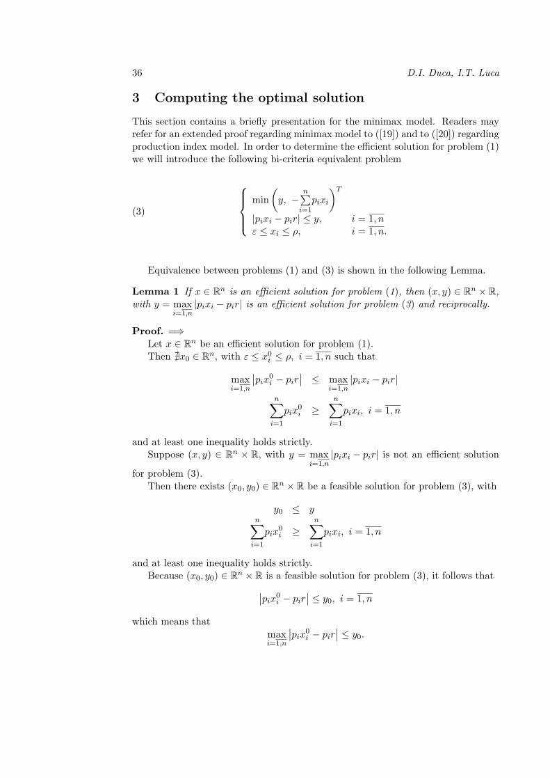
This section contains a briefly presentation for the minimax model. Readers mayrefer for an extended proof regarding minimax model to ([19]) and to ([20]) regardingproduction index model. In order to determine the efficient solution for problem (1)we will introduce the following bi-criteria equivalent problem

(3)

min

(y, −

n∑i=1pixi

)T

|pixi − pir| ≤ y, i = 1, nε ≤ xi ≤ ρ, i = 1, n.

Equivalence between problems (1) and (3) is shown in the following Lemma.

Lemma 1 If x ∈ Rn is an efficient solution for problem (1), then (x, y) ∈ Rn × R,with y = max

i=1,n|pixi − pir| is an efficient solution for problem (3) and reciprocally.

Proof. =⇒Let x ∈ Rn be an efficient solution for problem (1).

Then @x0 ∈ Rn, with ε ≤ x0i ≤ ρ, i = 1, n such that

maxi=1,n

∣∣pix0i − pir∣∣ ≤ max

i=1,n|pixi − pir|

n∑i=1

pix0i ≥

n∑i=1

pixi, i = 1, n

and at least one inequality holds strictly.Suppose (x, y) ∈ Rn × R, with y = max

i=1,n|pixi − pir| is not an efficient solution

for problem (3).Then there exists (x0, y0) ∈ Rn × R be a feasible solution for problem (3), with

y0 ≤ yn∑

i=1

pix0i ≥

n∑i=1

pixi, i = 1, n

and at least one inequality holds strictly.

Because (x0, y0) ∈ Rn × R is a feasible solution for problem (3), it follows that∣∣pix0i − pir∣∣ ≤ y0, i = 1, n

which means that

maxi=1,n

∣∣pix0i − pir∣∣ ≤ y0.


Thus we obtain that

maxi=1,n

∣∣pix0i − pir∣∣ ≤ y0 ≤ y = max

i=1,n|pixi − pir|

n∑i=1

pix0i ≥

n∑i=1

pixi, i = 1, n

and at least one inequality holds strictly.This way we obtain a contradiction for the efficiency of x ∈ Rn as solution for

(1).In conclusion, (x, y) ∈ Rn × R, with y = max

i=1,n|pixi − pir| is an efficient solution

for problem (3).⇐=

Let (x, y) ∈ Rn×R, with y = maxi=1,n

|pixi − pir| be an efficient solution for problem

(3).Suppose x ∈ Rn is not an efficient solution for problem (1) and let x0 be a feasible

solution, with

maxi=1,n

∣∣pix0i − pir∣∣ ≤ max

i=1,n|pixi − pir| , i = 1, n

n∑i=1

pix0i ≥

n∑i=1

pixi, i = 1, n

and at least one inequality holds strictly.Denoting y0 = max

i=1,n

∣∣pix0i − pir∣∣ , it follows

y0 ≤ yn∑

i=1

pix0i ≥

n∑i=1

pixi, i = 1, n

and at least one inequality holds strictly, which contradicts the efficiency of (x, y) ∈Rn × R.

In conclusion x ∈ Rn is an efficient solution for problem (1) and this ends ourproof.

Using results of Yu ([34]), Bot ([3]) and Geoffrion ([11]) the bi-criteria problem(3) is equivalent to the following parametric optimization problem

(4)

min

λy − (1− λ)

n∑i=1pixi

|pixi − pir| ≤ y, i = 1, nε ≤ xi ≤ ρ, i = 1, n.

with λ ∈ (0, 1) and the following Lemma holds.


Lemma 2 (x, y) ∈ Rn ×R is an efficient solution for bi-criteria problem (3) if andonly if ∃λ ∈ (0, 1) such that (x, y) ∈ Rn × R is an optimal solution for parametricoptimization problem (4)

The meaning of in this context is the sensitivity of energy plant for reducingthe fluctuation. The bigger is, the energy plant is more interested in reducingthe fluctuation. The smaller is, the energy plant is less interested in reducing thefluctuation and more interested in increasing the turnover.

Considering the equivalence between problems (1) and (3), respectively problems(3) and (4), it follows from transitivity that problems (1) and (4) are equivalent. Thismeans that in order to compute the efficient solution for (1) we have to determinethe optimal solution for (4). In the process of computing the optimal solution,we will split the set 1, 2, ..., n in subsets like 1, 2, ..., l and l + 1, l + 2, ..., n,or 1, 2, ..., l, l + 1, l + 2, ...,m and m+ 1,m+ 2, ..., n. If price is constant onsuch an interval, it will be denoted by p.

Theorem 1 The optimal solutions for parametric optimization problem (4) are:

1. If λ < nn+1 , then

x∗i = ρ, i = 1, ny∗ = p (ρ− r)

or

• if p1 ≤ pj , j = l + 1, n, then

x∗i = ρ, i = 1, l

x∗j = r + y∗

pj, j = l + 1, n

y∗ = p (ρ− r)

where p1 = pi, i = 1, l.

• else problem has no solution.

2. If λ = nn+1 , then x∗i = r + y∗

pi, i = 1, n

y∗ = mini=1,n

pi (ρ− r) .

3. If λ > nn+1 , then

x∗i = r, i = 1, ny∗ = 0.

4. If λ < ll+1 , then


• if pj < p, j = l + 1, n, thenx∗i = ρ, i = 1, l

x∗j = ρ, j = l + 1, n

y∗ = p (ρ− r)



5. If λ = ll+1 , then

• if pj < pi, i = 1, l, j = l + 1, n, thenx∗i = r + y∗

pi, i = 1, l

x∗j = ρ, j = l + 1, n

y∗ = mini=1,l

pi (ρ− r) , if pj < pi.

• else problem has no solution

6. If λ < l+(n−m)l+(n−m)+1 , then

• if pj ≤ p ≤ pi, i = 1, l, j = l + 1,m, thenx∗i = r + y∗

pi, i = 1, l

x∗j = ρ, j = l + 1,m

x∗k = ρ, k = m+ 1, ny∗ = p (ρ− r)

where p3 = pk, k = m+ 1, n.


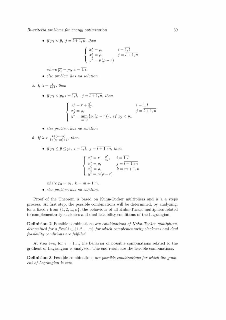
Proof of the Theorem is based on Kuhn-Tucker multipliers and is a 4 stepsprocess. At first step, the possible combinations will be determined, by analyzing,for a fixed i from 1, 2, ..., n, the behaviour of all Kuhn-Tucker multipliers relatedto complementarity slackness and dual feasibility conditions of the Lagrangian.

Definition 2 Possible combinations are combinations of Kuhn-Tucker multipliers,determined for a fixed i ∈ 1, 2, ..., n for which complementarity slackness and dualfeasibility conditions are fulfilled.

At step two, for i = 1, n, the behavior of possible combinations related to thegradient of Lagrangian is analyzed. The end result are the feasible combinations.

Definition 3 Feasible combinations are possible combinations for which the gradi-ent of Lagrangian is zero.


At step three, for i = 1, n, the combining capacity of feasible combinations isanalyzed. The end result are the critical combinations.

Definition 4 Critical combinations are those feasible combinations for which a so-lution does not exist if they are combined.

At step four, the optimal solutions are computed based on feasible and criticalcombinations.Proof. of Theorem 1 . Let λ ∈ (0, 1) fixed. Problem (4) is equivalent with thefollowing

min

λy − (1− λ)

n∑i=1pixi

−y ≤ pixi − pir, i = 1, npixi − pir ≤ y, i = 1, nε ≤ xi, i = 1, nxi ≤ ρ, i = 1, n

which is a convex optimization problem with inequality constraints.The associated Kuhn-Tucker conditions are

(KT1) ∂L∂xi

= − (1− λ) pi − aipi + bipi − ci + di = 0, i = 1, n

(KT2) ∂L∂y = λ−

n∑i=1ai −

n∑i=1bi = 0

(KT3) (−y∗ − pix∗i + pir) ai = 0, ai ≥ 0, i = 1, n

(KT4) (pix∗i − pir − y∗) bi = 0, bi ≥ 0, i = 1, n

(KT5) (ε− x∗i ) ci = 0, ci ≥ 0, i = 1, n

(KT6) (x∗i − ρ) di = 0, di ≥ 0, i = 1, n

where

L : Rn × R× Rn × Rn × Rn × Rn −→ R

L (x, y, a, b, c, d) = λy − (1− λ)

n∑i=1

pixi +

n∑i=1

ai (−y − pixi + pir) +

n

+∑i=1

bi (pixi − pir − y) +

+n∑

i=1

ci (ε− xi) +n∑

i=1

di (xi − ρ)

is the associated Lagrangian and (x∗, y∗) ∈ Rn × R is the optimal solution.


Remark 1 Due to the fact that the optimization problem is a convex one, it followsthat Kuhn-Tucker conditions are both necessary and sufficient.

We have to compute (x∗, y∗) ∈ Rn×R in order to determine the optimal solutionfor our parametric problem (4).

Step 1Let i ∈ 1, 2, ...n fixed. Then, the possible scenarios for Kuhn-Tucker multipliersare

Kuhn-Tucker multipliers

Scenarios ai bi ci di1 =0 =0 =0 =0

2 > 0 =0 =0 =0

3 =0 > 0 =0 =0

4 =0 =0 > 0 =0

5 =0 =0 =0 > 0

6 > 0 > 0 =0 =0

7 > 0 =0 > 0 =0

8 > 0 =0 =0 > 0

9 =0 > 0 > 0 =0

10 =0 > 0 =0 > 0

11 =0 =0 > 0 > 0

12 > 0 > 0 > 0 =0

13 > 0 > 0 =0 > 0

14 =0 > 0 > 0 > 0

15 > 0 =0 > 0 > 0

16 > 0 > 0 > 0 > 0

We will analyze the behavior of each scenario related to complementarity slack-ness and dual feasibility conditions (Kuhn-Tucker conditions (KT3) to (KT6)) andwe will determine the solution for each scenario if it exists. We will analyze in detailonly scenario 1

ai = 0 bi = 0 ci = 0 di = 0The system generated by Kuhn-Tucker conditions (KT3) to (KT6) is

(5)

−y∗ ≤ pix

∗i − pir

pix∗i − pir ≤ y∗

x∗i ≥ εx∗i ≤ ρ.

From the first two inequalities of the system we have

x∗i ≥ r − y∗

pi

x∗i ≤ r +y∗

pi


and considering the last two inequalities of the system it follows that

y∗ ≤ pi (r − ε)

y∗ ≤ pi (ρ− r) .

Thus, in case of scenario 1, the solution for system (5) isx∗i ∈

[r − y∗

pi, r + y∗

pi

]y∗ ≤ pi (r − ε)y∗ ≤ pi (ρ− r) .

From the 16 scenarios, we have proved that only 8 are possible combinations.These are 1, 2, 3, 4, 5, 6, 7 and 10.

Step 2For i = 1, n we will analyze the behavior of possible combinations related to the

gradient of Lagrangian (Kuhn-Tucker conditions (KT1) and (KT2)). In detail wewill present scenario 6.

ai > 0 bi > 0 ci = 0 di = 0The system generated by Kuhn-Tucker conditions (KT1) and (KT2) is − (1− λ) pi − aipi + bipi = 0, i = 1, n

λ−n∑

i=1ai −

n∑i=1bi = 0

and thusai = bi − (1− λ) , i = 1, n.

It follows thatn∑

i=1

ai =

n∑i=1

bi − n (1− λ) .

But ai > 0, i = 1, n and then bi > (1− λ) , i = 1, n.In conclusion we get

λ >n

n+ 1.

Synthesizing the behavior of the 8 possible combinations related to Kuhn-Tuckerconditions (KT1) and (KT2)) the following situation is obtained

Scenario Solution (KT1) (KT2)

1 @ × ×2 @ × ×3 ∃, if λ = n

n+1 X X4 @ × ×5 @ X ×6 ∃, if λ > n

n+1 X X7 @ × ×10 ∃, if λ < n

n+1 X X


Remark 2 For scenario 5 we notice that (KT2) is not satisfied, which means thatscenario 5 will not generate a solution by it’s own, but may be combined with othersto generate solution.

Thus, the feasible scenarios which will generate the optimal solution for (4) are3, 5, 6 and 10.

Step 3

We state that the critical combinations are 6 with 5 and 6 with 10. Readersmay find an extended proof in ([19]). Same reference contains a proof that order ofscenarios in a combination does not change the solution.

Step 4

The combinations based on which we will compute the optimal solution for (4)are 3, 6, 10, 6+3, 10+3, 10+5, 3+5 and 3+5+10. We will analyze combination 10+3,the others being similar. They are extensively described in ([19]). For combination10 with 3, if i = 1, l and j = l + 1, n, then Kuhn-Tucker conditions (KT1) and (KT2)will be

− (1− λ) pi + bipi + di = 0, i = 1, l

− (1− λ) pj + bjpj = 0, j = l + 1, n

λ−l∑

i=1bi −

n∑j=l+1

bj = 0.

Thus

di = pi [(1− λ)− bi] , i = 1, l

and because di > 0, i = 1, l it follows that

l∑i=1

bi < l (1− λ) .

Also

bj = (1− λ) , j = l + 1, n

and thenn∑

j=l+1

bj = (n− l) (1− λ)

Using now the last equation of the system it follows

λ <n

n+ 1.

For 10, with i = 1, l the solution isx∗i = ρ, i = 1, l

y∗ = pi (ρ− r) , i = 1, l


and for 3, with j = l + 1, n the solution isx∗j = r + y∗

pj, j = l + 1, n

y∗ ≤ pj (ρ− r) , j = l + 1, n.

Because y∗ = pi (ρ− r) , i = 1, l we state that all prices are constant on the set1, 2, ...l and denote p1 = pi, i = 1, l. In order to have all conditions for y∗ fulfilledit is necessary that

p1 ≤ pj , j = l + 1, n.

Chosing

y∗ = p1 (ρ− r)

an optimal solution for (4) isx∗i = ρ, i = 1, l

x∗j = r + y∗

pj, j = l + 1, n

y∗ = p1 (ρ− r) , if p1 ≤ pj .

if λ < nn+1 .

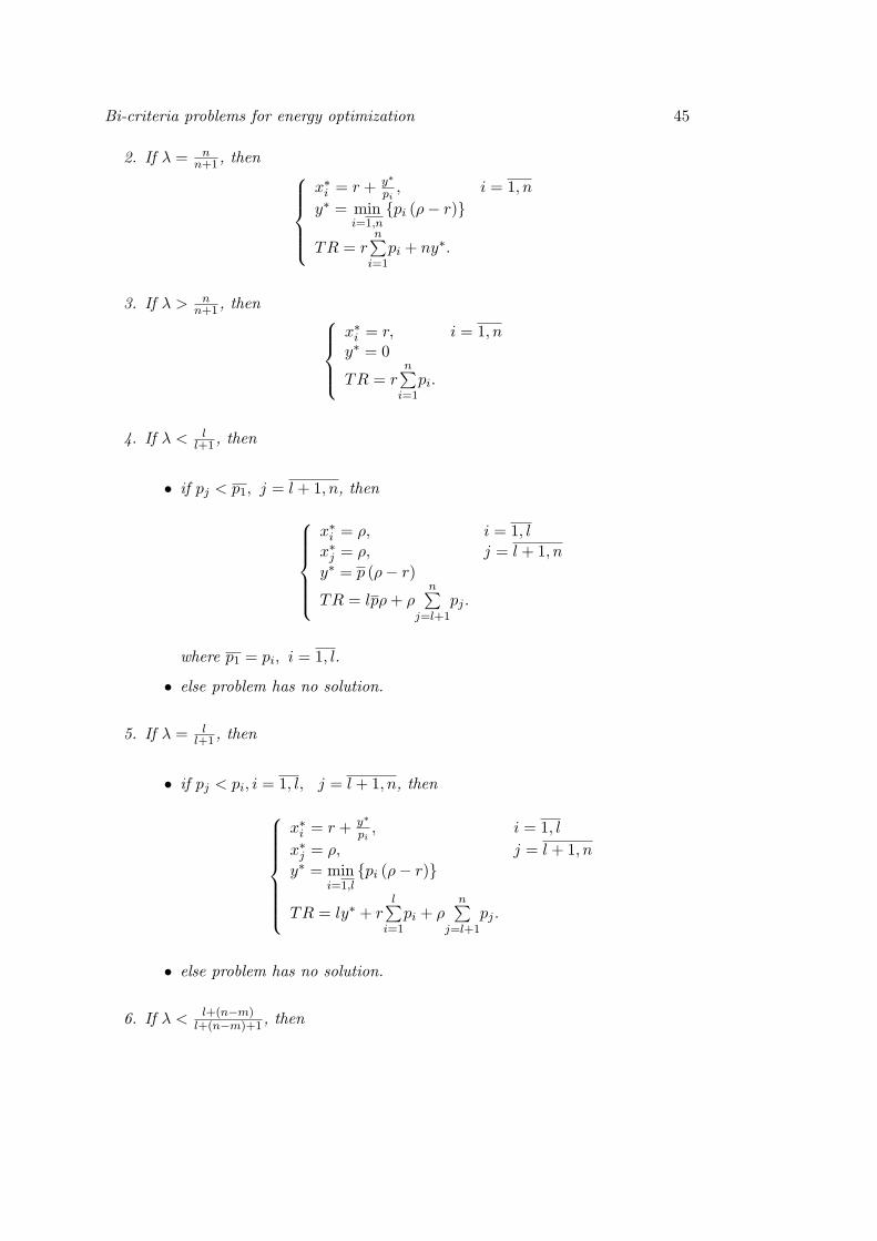
Denoting by TR the turnover, using Theorem 1 and the equivalence betweenproblems (1), (3) and (4), the following is true

Theorem 2 The efficient solution for bi-criteria energy optimization problem (1)is

1. If λ < nn+1 , then

x∗i = ρ, i = 1, ny∗ = p (ρ− r)TR = npρ

or

• if p1 ≤ pj , j = l + 1, n, then

x∗i = ρ, i = 1, l

x∗j = r + y∗

pj, j = l + 1, n

y∗ = p1 (ρ− r)

TR = lp1ρ+ rn∑

j=l+1

pj + (n− l) y∗.




2. If λ = nn+1 , then

x∗i = r + y∗

pi, i = 1, n

y∗ = mini=1,n

pi (ρ− r)

TR = rn∑

i=1pi + ny∗.

3. If λ > nn+1 , then

x∗i = r, i = 1, ny∗ = 0

TR = rn∑

i=1pi.

4. If λ < ll+1 , then

• if pj < p1, j = l + 1, n, then

x∗i = ρ, i = 1, l

x∗j = ρ, j = l + 1, n

y∗ = p (ρ− r)

TR = lpρ+ ρn∑

j=l+1

pj .



5. If λ = ll+1 , then

• if pj < pi, i = 1, l, j = l + 1, n, then

x∗i = r + y∗

pi, i = 1, l

x∗j = ρ, j = l + 1, n

y∗ = mini=1,l

pi (ρ− r)

TR = ly∗ + rl∑

i=1pi + ρ

n∑j=l+1

pj .


6. If λ < l+(n−m)l+(n−m)+1 , then


• if pj ≤ p3 ≤ pi, i = 1, l, j = l + 1,m, then

x∗i = r + y∗

pi, i = 1, l

x∗j = ρ, j = l + 1,m

x∗k = ρ, k = m+ 1, ny∗ = p (ρ− r)

TR = ly∗ + rl∑

i=1pi + ρ

n∑j=l+1

pj + (n−m) pρ.

where p3 = pk, k = m+ 1, n.


4 Conclusion

Both models are sensitive to input data. A small change of parameters in theconstraint system can change completely the solution. Due to predefined level andthe form for measure of fluctuation, Minimax model has a limited optimizationrange. Our models may provide the framework for optimization of power grids.

References

[1] Best M.J., Grauer R.R., Sensitivity analysis for mean-variance portfolio prob-lems, Management Science, vol. 37, no. 8, 1991, pp. 980-989.

[2] Best M.J., Grauer R.R., On the sensitivity of mean-variance efficient portfoliosto changes in asset means: Some analytical and computational results, Reviewof Financial Studies, vol. 4, no. 2, 1991, pp. 315-342.

[3] Bot I.R., Grad S.M., Wanka G., Duality in Vector Optimization, Springer, 2009.

[4] Cai X., Teo K-L., Yang X., Zhou X.Y., Portfolio optimization under a minimaxrule, Management Science, vol. 46, no. 7, 2000, pp. 957-972.

[5] Chopra V.K., Hensel C.R., Turner A.L., Massaging mean-variance inputs: re-turns from alternative global investment strategies in the 1980s, ManagementScience, vol. 39, no. 7, 1993, pp. 845-855.

[6] Constantinides G.M., Capital market equilibrium with transactions costs, Jour-nal of Political Economy, vol. 94, no. 4, 1986, pp. 842-862.

[7] Dumas B., Luciano E., An exact solution to a dynamic portfolio choice problemunder transaction costs, Journal of Finance, vol. 46, no. 2, 1991, pp. 577-595.

[8] Elton E.J., Gruber M.J., The multi-period consumption investment problemand single period analysis, Oxford Economic Papers, vol. 26, no. 2, 1974, pp.289-301.


[9] Elton E.J., Gruber M.J.,On the optimality of some multiperiod portfolio selec-tion criteria, Journal of Business, vol. 47, no. 2, 1974, pp. 231-243.

[10] Fama F., Multiperiod consumption-investment decision, American EconomicReview, vol. 60, no. 1, 1970, pp. 163-174.

[11] Geoffrion M.A., Proper Efficiency and the Theory of Vector Maximization, Jour-nal of Mathematical Analysis and Applications, vol. 22, no. 3, 1968, pp. 618-630.

[12] Hakkanson N.H., Multiperiod mean variance analysis: Toward a general theoryof portfolio choice, Journal of Finance, vol. 26, no. 4, 1971, pp. 857-884.

[13] Huang X., Qiao L., A risk index model for multiperiod uncertain portfolio se-lection, Information Science, vol. 217, 2012, pp. 108-116.

[14] Konno H., Yamazaki H., Mean absolute deviation portfolio optimization modeland its applications to Tokyo Stock Market, Management Science, vol. 37, no.5, 1991, pp. 519-531.

[15] Lee C.F., Finnerty J.E., Wort D.H., Index models for portfolio selection, Hand-book of Quantitative Finance and Risk Management, 2010, pp. 111-124.

[16] Leith C. Numerical simulation of the earth’s atmosphere, Methods in Compu-tational Physics, 1965, pp. 1-28

[17] Li D., Ng W.L., Optimal dynamic portfolio selection: Multiperiod mean-variance formulation, Mathematical finance, vol. 10, no. 3, 2000, pp. 387-406.

[18] Li J., Mahalov A., Hyde P., Impacts of agricultural irrigation on ozone con-centrations in the Central Valley of California and in the contiguous UnitedStates based on WRF-Chem simulations, Agricultural and Forest Meteorology,vol. 221, 2016, pp. 34-49.

[19] Mahalov A., Luca T.I., Minimax rule for energy optimization, Computers andFluids (accepted for publication)

[20] Mahalov A., Luca T.I., Production index for energy optimization, Optimizationand Engineering (submited for publication)

[21] Markowitz H., Portfolio selection, The Journal of Finance, vol. 7, no. 1, 1952,pp. 77-91.

[22] Merton C., Lifetime portfolio selection under uncertainty: the continuous timecase, Review of Economics and Statistics, vol. 51, no. 4, 1972, pp. 247-257.

[23] Mossin J., Optimal multiperiod portfolio policies, Journal of Business, vol. 41,no. 2, 1968, pp. 215-229.


[24] Ruddell B., Salamanca F., Mahalov A., Reducing a semiarid city’s peak electri-cal demand using distributed cold thermal energy storage, Applied Energy, vol.134, 2014, pp. 35-44.

[25] Perold A.F., The implementation shortfall: Paper versus reality, Journal ofPortfolio Management, vol. 14, no. 3, 1988, pp. 4-9.

[26] Phillips N., The general circulation of the atmosphere: a numerical experiment,Quarterly Journal of the Royal Meteorological Society, vol 82, 1956, pp. 123-154.

[27] Salamanca F., Georgescu M., Mahalov A., Moustaoui M., Wang M., Anthro-pogenic heating of the urban environment due to air conditioning, Journal ofGeophysical Research: Atmospheres, American Geophysical Union, vol. 119(10), 2014, pp. 5949-5965.

[28] Samuelson A., Lifetime portfolio selection by dynamic stochastic programming,Review of Economics and Statistics, vol. 51, no. 3, 1969, pp. 239-246.

[29] Sharpe W., A simplified model for portfolio analysis, Management Science, vol.9, no. 2, 1963, pp. 277-293.

[30] Sharpe W., A linear programming algorithm for a mutual fund portfolio selec-tion, Management Science, vol. 13, no. 7, 1967, pp. 499-510.

[31] Sharpe W., A linear programming approximation for general portfolio selectionproblem, Journal of Finance and Quantitative Analysis, vol. 6, no.5, 1971, pp.1263-1275.

[32] Smith K.V., A transaction model for portfolio revision, Journal of Finance, vol.22, no. 3, 1967, pp. 425-439.

[33] Stone B.K., A linear programming formulation of the general portfolio selectionproblem, vol. 8, no. 4, 1973, pp. 621-636.

[34] Yu P.L., Cone convexity, cone extreme points and nondominated solutions indecision problems with multiobjectives, Journal of Optimization Theory andApplications, vol. 14, no. 3, 1974, pp. 319-377.

Dorel I. DucaBabes Bolyai UniversityFaculty of Mathematics and Computer ScienceDepartment of MathematicsKogalniceanu street 1, Cluj Napoca, [email protected]

Ionut Traian LucaBabes Bolyai UniversityFaculty of BusinessDepartment of BusinessHorea street 7, Cluj Napoca, [email protected]


On a Markov method 1

Ioan Tincu

Abstract

This paper contains a new approach a transformed Markov.

2010 Mathematics Subject Classification: 40A05, 40B05.Key words and phrases: Method Markov, convergent series.

1 Introduction

Let

∞∑k=1

A(k) a series of real numbers convergence with the sum A,

∞∑k=1

A(k) = A.

The method of A.A.Markov consists in expansion of every term A(k) in, conver-gent series,

A(k) =

∞∑k=1

a(k)i , A =

∞∑k=1

A(k) =

∞∑k=1

∞∑i=1

a(k)i =

∞∑i=1

Ai, Ai =∑k≥1

a(k)i ,

when all the series from the columns Ai are convergent.

2 Main result

Continue presents a new approach of method Markov.

Theorem 1 Let∞∑n=0

an a real series convergent and f, g : [0,∞) × [0,∞) → R two

functions which verify:i) f(0, n) = an, (∀)n ∈ N,ii) f(i+ 1, j)− f(i, j) = g(i, j + 1)− g(i, j), (∀)i ∈ 0, 1, ..., j, j ∈ N.

If limn→∞

n∑j=0

g(j, n+ 1) = 0 then

∞∑j=0

aj =

∞∑j=0

[f(j + 1, j) + g(j, j)].


49

50 I. Tincu

Proof. We have

f(j + 1, j)− f(0, j) =

j∑i=0

[f(i+ 1, j)− f(i, j)] =

j∑i=0

[g(i, j + 1)− g(i, j)]

Note

aj = f(j + 1, j) +

j∑i=0

[g(i, j)− g(i, j + 1)].

Therefore,n∑

j=0

aj =

n∑j=0

f(j + 1, j) +

n∑j=0

j∑i=0

[g(i, j)− g(i, j + 1)].

In formulan∑

j=0

j∑i=0

Ai,j =

n∑j=0

n∑i=j

Aj,i,

we will consider

Ai,j = g(i, j)− g(i, j + 1),

and we will obtain

n∑j=0

aj =

n∑j=0

f(j + 1, j) +

n∑j=0

n∑i=j

[g(j, i)− g(j, i+ 1)]

=

n∑j=0

f(j + 1, j) +

n∑j=0

[g(j, j)− g(j, n+ 1)]

=

n∑j=0

[f(j + 1, j) + g(j, j)]−n∑

j=0

g(j, n+ 1).

Since limn→∞

n∑j=0

g(j, n+ 1) = 0, it followsn∑

j=0

aj =n∑

j=0

[f(j + 1, j) + g(j, j)].

Propertie 1 The following relation

(1)

(n+ j − 2

j

)≥ j, (∀)j ∈ N

holds.

Proof. In order to prove this relation we will use mathematical induction.

For j = 1 we have

(n+ 3

1

)≥ 1, 1 ≥ 1.

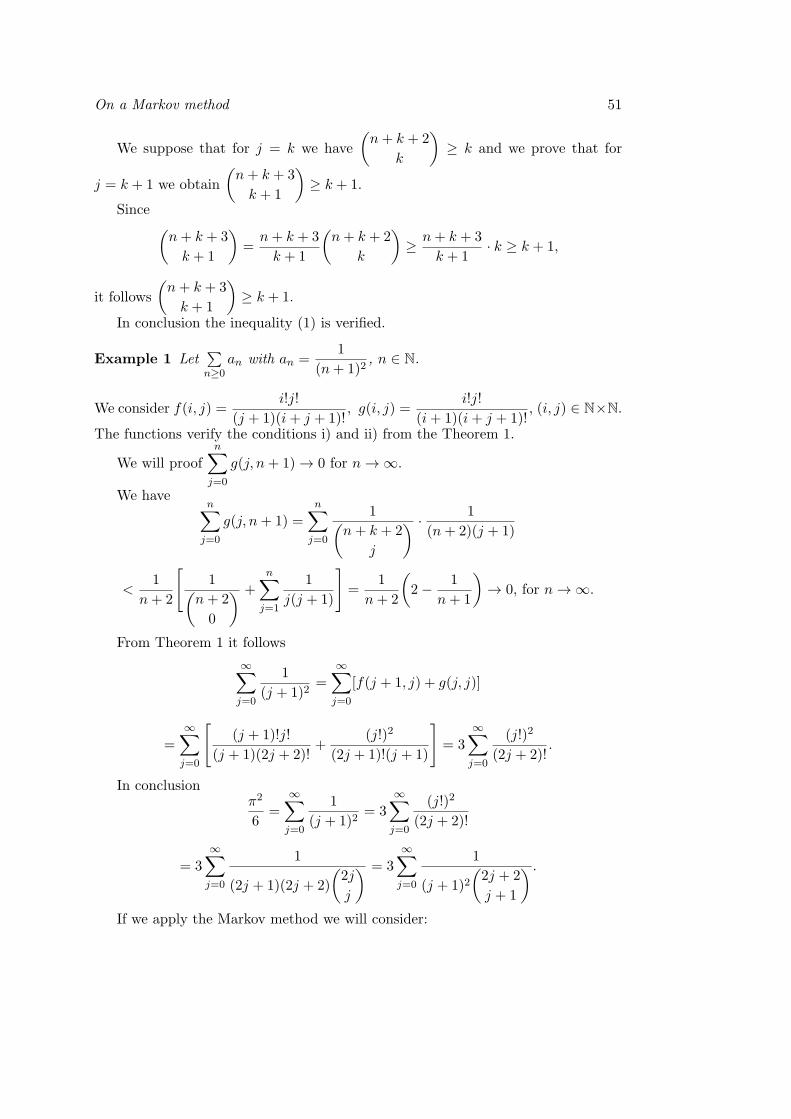
On a Markov method 51

We suppose that for j = k we have

(n+ k + 2

k

)≥ k and we prove that for

j = k + 1 we obtain

(n+ k + 3

k + 1

)≥ k + 1.

Since (n+ k + 3

k + 1

)=n+ k + 3

k + 1

(n+ k + 2

k

)≥ n+ k + 3

k + 1· k ≥ k + 1,

it follows

(n+ k + 3

k + 1

)≥ k + 1.

In conclusion the inequality (1) is verified.

Example 1 Let∑n≥0

an with an =1

(n+ 1)2, n ∈ N.

We consider f(i, j) =i!j!

(j + 1)(i+ j + 1)!, g(i, j) =

i!j!

(i+ 1)(i+ j + 1)!, (i, j) ∈ N×N.

The functions verify the conditions i) and ii) from the Theorem 1.

We will proof

n∑j=0

g(j, n+ 1) → 0 for n→ ∞.

We haven∑

j=0

g(j, n+ 1) =n∑

j=0

1(n+ k + 2

j

) · 1

(n+ 2)(j + 1)

<1

n+ 2

[1(

n+ 2

0

) +

n∑j=1

1

j(j + 1)

]=

1

n+ 2

(2− 1

n+ 1

)→ 0, for n→ ∞.

From Theorem 1 it follows

∞∑j=0

1

(j + 1)2=

∞∑j=0

[f(j + 1, j) + g(j, j)]

=∞∑j=0

[(j + 1)!j!

(j + 1)(2j + 2)!+

(j!)2

(2j + 1)!(j + 1)

]= 3

∞∑j=0

(j!)2

(2j + 2)!.

In conclusionπ2

6=

∞∑j=0

1

(j + 1)2= 3

∞∑j=0

(j!)2

(2j + 2)!

= 3∞∑j=0

1

(2j + 1)(2j + 2)

(2j

j

) = 3∞∑j=0

1

(j + 1)2(2j + 2

j + 1

) .If we apply the Markov method we will consider:

52 I. Tincu

i)∑n≥1

1

n(n+ 1)...(n+ k)=

1

k · k!,

ii) a(k)i =

(i− 1)!

k(k + 1)...(k + i),

iii) Ai =∑k≥1

aki = (i− 1)!∑k≥1

1

k(k + 1)...(k + i)=

= (i− 1)!∑k≥1

[1

k(k + 1)...(k + i− 1)− 1

(k + 1)...(k + i)

]· 1i=

(i− 1)!

i · i!=

1

i2,

∞∑i=1

Ai =

∞∑i=1

1

i2=π2

6=∑i≥1

∑k≥1

a(k)i .

References

[1] G. M. Fihtenholt, Curs de calcul diferential si integral, E.T.Bucuresti, vol.II,1964.

[2] G.H.Hardy, Divergent series, At the Clarendon Press, Oxford, 1949.

Ioan TincuUniversity Lucian Blaga of SibiuFaculty of ScienceDepartament of MathematicsStr. Dr. I. Ratiu, No. 5-7 550012 Sibiu Romaniae-mail: [email protected]


About a category of abelian groups 1

Teodor Dumitru Valcan

Abstract

We say that an R-module (abelian group) M has the direct summand in-tersection property (in short D.S.I.P.) if the intersection of any two direct sum-mands ofM is again a direct summand inM . In this work we will present threeclasses of abelian groups (torsion, divisible, respectively torsion-free) which havethe property that any proper subgroup has D.S.I.P. and we are going to showthat there are not such mixed groups.

2010 Mathematics Subject Classification: 13D30, 43A70.Key words and phrases: R-module, abelian group, Frattini subgroup.

1 Short history and introduction

Let R be an associative ring, with unity. We say that an R-module (abeliangroup) M has the direct summand intersection property, in short D.S.I.P., if theintersection of any two direct summand of M is again a direct summand in M . TheR-modules (the abelian groups) with D.S.I.P. have been studied in [1]-[3], [5], [6] and[8]-[17]. In this work we will present three classes of abelian groups (torsion, divisible,respectively torsion-free) which have the property that any proper subgroup hasD.S.I.P. and we are going to show that there are not mixed groups with this property.We shall call these groups ”groups with the property (P )”.

In this context, all through this paper by group we mean abelian group in additivenotation and we will use the classic notations:

- P - for the set of all prime numbers,- r(A) - for the rank of a group A,- t(A) - for the type of a torsion-free group A,- F (A) - for the Frattini subgroup of a group A (see [10]),- |I| - for the cardinal of a set I.For the beginning we make the remark that, according to the proofs in [10], it

follows:1Received 30 June, 2016Accepted for publication (in revised form) 01 October, 2016

53

54 T.D. Valcan

Remark 1 Let G be an abelian group.

1) If G has D.S.I.P., then no any their (proper) subgroup has D.S.I.P..

2) If any proper subgroup of G has D.S.I.P. and G has a (direct) decompositionin fully invariant direct summands, then G has D.S.I.P..

3) If G has D.S.I.P., then no any quotient group of G has D.S.I.P..

4) If any nontrivial quotient group of group G has D.S.I.P. and G has a (direct)decomposition in fully invariant direct summands, then G has D.S.I.P..

5) Let B be a (proper) subgroup of G. If B and G/B have D.S.I.P., then it doesnot follow that G has D.S.I.P..

Proof. 1) Counterexample: let p be a prime number and let be G = Z(p)⊕Z(p∞)and B = Z(p)⊕C, where C = ⟨c2⟩, and c2 is a generator of Z(p∞) with the propertythat p2c2 = 0; so C ∼= Z(p2). Then, according to [6,Theorem 2], G has D.S.I.P., butB doesn’t have this property anymore.

2) Let G be a group with the property that any proper subgroup has D.S.I.P. and

let G =⊕i∈I

Gi be a direct decomposition of G in fully invariant direct summands.

Then the hypothesis and [6,Lemma 1] show that G has D.S.I.P., too.

3) Counterexample: let G = Q ⊕ Q and B = Z. Then, according to [8,Lemma4.1 and Corollary 2.2], G and B have D.S.I.P., but [6,Theorem 2] shows that G/B =

(Q/Z)⊕ (Q/Z) =⊕p∈P

(Z(p∞)⊕ Z(p∞)) does not have this property.

4) Let G be a group with the property that any quotient group (of G) has

D.S.I.P. and, as to the point 2), let G =⊕i∈I

Gi be a direct decomposition of G in

fully invariant direct summands. Then the hypothesis shows that, for every i ∈ I,Gi has D.S.I.P.. Again [6,Lemma 1] shows that G has D.S.I.P., too.

5) Counterexample: let be G = Z(p2) ⊕ Z(p∞) ⊕ Z(q∞), where p and q aretwo distinct prime numbers. Then F (G) = Z(p∞) ⊕ Z(q∞) and G/F (G) ∼= Z(p2).According to [8,Remark 3.6] and to [6,Theorem 2], F (G) and G/F (G) have D.S.I.P.,but G does not have this property.

2 Torsion groups

We begin the determination of the torsion groups with the property (P ) withthe determination of the p-groups with this property.

Theorem 1 The following statements are equivalent for a p-group G:

a) G has the property (P ).

b) either

i) G is indecomposable non-elementary, (1)or

ii) G is elementary, (2)or


iii) G = Z(p2)⊕Z(p). (3)

Proof. a) implies b) Let G be a p-group with the property that any proper subgrouphas D.S.I.P.. IfG is either indecomposable or elementary, then this gives the requiredresult. So that we suppose that G is not a such group. If there is g ∈ G[p] such thathp(g) = k, where 1 ≤ k < ∞, then g ∈ pkG and g ∈ pk+1G. It follows that there isa ∈ G such that g = pka. Since pg = 0, it follows that o(a) = k + 1 and accordingto [4,Corollary 27.2], ⟨a⟩ is a direct summand in G, that is G = ⟨a⟩ ⊕ B. Now wedistinguish two cases.

Case 1: For any b ∈ B[p], ⟨b⟩ is a direct summand in B. Then B[p] is a directsummand in B. We suppose that B = B[p]⊕C. But C[p] = C ∩B[p] = 0; so C = 0and B = B[p]. It follows that there is a cardinal mp such that, up to isomorphism,G = Z(pk+1) ⊕ (⊕mpZ(p)). If k = mp = 1, then G = Z(p2)

⊕Z(p) is of the form

(3). If k ≥ 2, the subgroup Z(pk+1) ⊕ Z(p) does not have D.S.I.P., which is acontradiction to the hypothesis.

Case 2: There is a b1 ∈ B[p] such that ⟨b1⟩ is not a direct summand in B. Wechoose such a b1 ∈ B[p]. Then the subgroup ⟨a⟩⊕ ⟨b1⟩ does not have D.S.I.P. and Gdoes not have the property (P ) - again we obtain a contradiction to the hypothesis.

It follows that, for any g ∈ G[p], either hp(g) = 0 or hp(g) = ∞. So thedirect summands of G are either p-bounded or isomorphic to Z(p∞). So, G =E⊕F , where pE = 0 and F is divisible. Then, according to the hypothesis and to

[6,Theorem 2], it follows that F = Z(p∞) and G is a p-group with D.S.I.P.. So thereis a cardinal mp such that G = (⊕mpZ(p)) ⊕ Z(p∞). We suppose that Z(p∞) =⟨c1, c2, . . . , cn, . . .⟩, with relationships pc1 = 0, pc2 = c1, . . . , pcn = cn−1, . . . and alsowe consider the subgroup K = Z(p) ⊕ ⟨c2⟩. Then the subgroup K does not haveD.S.I.P. - again we obtain a contradiction to the hypothesis. In conclusion F = 0and G is elementary.

b) implies a) If G is a group as in the statement, then either

i) G = Z(pn), (4)or

ii) G = Z(p∞), (5)or

iii) G = ⊕mpZ(p), (6)or G is of the form (3), where n ∈ N∗, 2 ≤ n < ∞ and mp is any cardinal. If G isof the form (3) it has the property (P), because any proper subgroup of G is eitherindecomposable or elementary. If G is either of the form (4) or of the form (5), thenany subgroup of G is indecomposable, so any subgroup of G has, in a trivial way,D.S.I.P.. If G is of the form (6), then any subgroup of G is of the same form, so anysubgroup of G has D.S.I.P..

From the above theorem and from [6,Theorem 2] it follows the following remarks:

Remark 2 a) If G is a p-group with D.S.I.P., then no any subgroup of G has thesame property.

56 T.D. Valcan

b) Generally, the p-groups with the property (P ) not coincide with these withD.S.I.P. with this property.

Now we can present the structure of torsion groups with the property (P ).

Corollary 1 If G is a torsion group, then the following statements are equivalent:a) G has the property (P ).b) G is of the form

G = (⊕p∈P1

Ap)⊕ (⊕p∈P2

Bp)⊕ (⊕p∈P3

Cp)⊕ (⊕p∈P4

Dp), (7)

where:- P1, P2, P3 and P4 are subsets of the set P of all prime numbers, with the

property that P1 ∩ P2 = P1 ∩ P3 = P1 ∩ P4 = P2 ∩ P3 = P2 ∩ P4 = P3 ∩ P4 = ∅,- for every p ∈ P1, Ap is a reduced (non-elementary) indecomposable p-group,- for every p ∈ P2, Bp is an elementary p-group,- for every p ∈ P3, Cp is a p-group of the form (3),- for every p ∈ P4, Dp is an indecomposable divisible p-group.

Proof. a) implies b) Let G =⊕p∈P

Gp be a torsion group, decomposed according to

[4,Theorem 8.4]. According to the hypothesis, for every p ∈ P , any proper subgroupof Gp has D.S.I.P.. So, for every p ∈ P , Gp is either of the form (3) or (4) or (5) or(6) and G is of the form (7).

b) implies a) Conversely, let G be a group of the form (7) and let H be any

subgroup of G. Then [4,Theorem 18.1] shows that H =⊕p∈P

Hp, where, for every

p ∈ P , Hp = H ∩Gp, and Gp is the p-component of G. Since, for every p ∈ P , Hp

satisfies the conditions from (2.1), it follows that, for every p ∈ P , Hp has D.S.I.P..Then [6,Lemma 1] shows that H has D.S.I.P., too and G has the property (P ).

From the above proved facts and from [8,Corollary 3.3] we obtain:

Remark 3 a) If G is a torsion group with D.S.I.P., then no any proper subgroupof G has this property.

b) Generally, the torsion groups which have the property (P ) not coincide withthese with D.S.I.P. with this property.

3 Divisible groups

Now we shall pass to determination of the divisible groups with the property(P ). In this context we have the following result:

Proposition 1 If G is a divisible group, then the following statements are equiva-lent:


a) G has the property (P ).

b) G has one from the following forms:

i) G = Q, (8)or

ii) G = Q⊕Q, (9)or

iii) G =⊕

p∈P0Z(p∞), (10)

or

where P0 is a subset of the set P of all prime numbers.

Proof. a) implies b) Let G = (⊕m0Q) ⊕ (⊕p∈P0

Dp) be a divisible group, where: Q

is the additive group of rational numbers, m0 is the torsion-free rank of G, P0 is asubset of the set P of all prime numbers and, for every p ∈ P0, Dp is a divisiblep-group. According to the hypothesis and to [17,Proposition 6], either G = ⊕m0Q

or G =⊕p∈P0

Dp.

We suppose that G = ⊕m0Q and m0 ≥ 3. In this case we consider the subgroupH = Q ⊕ E ⊕ F , where E and F are (proper) subgroups of Q such that t(E) andt(F ) are incomparable. Then [5,Theorem 3.3] shows that H does not have D.S.I.P..It follows that if G is a divisible torsion-free group with the property (P ), then it iseither of the form (8) or of the form (9).

Otherwise: According to (4.1), Q⊕Q has an indecomposable subgroup H, ofrank 2. Then the subgroup B = H ⊕ Q does not have D.S.I.P., because there arehomomorphisms 0 = f : H → Q which are not monomorphisms.

We suppose that G is torsion. According to the hypothesis and to [8,Theorem4.4], G is of the form (10).

b) implies a) If G = Q, then any subgroup H of G is indecomposable, so H hasD.S.I.P.. If G is of the form (9), then any subgroup of G is either indecomposable(see (4.1)) or completely decomposable of rank r ≤ 2. In this case [6,Theorem 6]completes the proof. If G is torsion and H is any subgroup of G, then, following

the same reasoning as in (2.3), we obtain that H =⊕p∈P

Hp, where, for every p ∈ P ,

Hp is a subgroup of Z(p∞). It follows that, for every p ∈ P , Hp has D.S.I.P.. Again[8,Theorem 4.4] shows that H has D.S.I.P..

From (3.1) and [8,Theorem 4.4] we obtain:

Remark 4 a) If G is a divisible group with D.S.I.P., then not any subgroup of Ghas the same property.

b) The divisible groups which have the property that any proper subgroup hasD.S.I.P. coincide with these with D.S.I.P. with this property.

58 T.D. Valcan

4 Torsion-free groups

Before passing to determine the structure of the torsion-free abelian groups withthe property (P ), we will present several results, obtained in [16], concerning theindecomposable subgroups of some torsion-free groups, results which we need here.

(4.1): If I is any index set, with the property that |I| ≤ |P |, then the groupQ∗ = ⊕IQ has indecomposable subgroups of every rank m ≤ |I|.

(4.2): Let Hi|i ∈ I be a family of torsion-free groups such that, for every i ∈ I,there is Gi ≤ Hi, where Gi|i ∈ I is a family of reduced of rank one groups, withthe property that, for every i1, i2 ∈ I, i1 = i2, t(Gi1) and t(Gi2) are incomparable.

Then the group H =⊕i∈I

Hi has indecomposable subgroups of every rank m ≤ |I|.

(4.3): Let G = B ⊕ C be any group and A a subgroup of G. If C is free and Ais indecomposable, then either r(A) = 1 or A ⊆ B.

Now we shall pass to the determination of torsion-free groups with the property(P ). We begin with the following elementary result:

Remark 5 If G is a free group, then any subgroup of G has D.S.I.P..

Proof. According to [4,Theorem 14.5], any subgroup of a free group is a free group,too. Now [8,Corollary 2.2] completes the proof.

Proposition 2 Let be G = D ⊕ F , where D = 0 is divisible and F is free. Thenthe following statements are equivalent:

a) G has the property (P ).b) r(D) = 1 and F is of finite rank.

Proof. a) implies b) Let be G = D ⊕ F , where D = 0 is divisible and F is free.According to the hypothesis and to [5,Theorem 3.3], it follows that F is of finiterank.

If r(D) ≥ 2, then let B and C be two subgroups of D, such that t(Z) < t(B) <t(C) and let K = Z ⊕ B ⊕ C. Then K is a subgroup of G, which, according to[6,Theorem 6], does not have D.S.I.P. It follows that r(D) = 1.

Otherwise: If r(D) ≥ 2, then, according to (4.1), D has an indecomposablesubgroup H, of rank two. Since there are homomorphisms 0 = f : H → Z which arenot monomorphisms, in this case [5,Proposition 1] shows that the subgroup H ⊕ Zdoes not have D.S.I.P..

b) implies a) Let G = Q ⊕ F be a group as in the statement and let B be anysubgroup of G. According to (4.3), if B is indecomposable, then r(B) = 1 and Bhas D.S.I.P.. We suppose that r(B) ≥ 2. Then we distinguish three cases:

Case 1: Suppose that Q ≤ B. Then B = Q ⊕ E, where E = F ∩ B is a freegroup and r(E) ≥ 1. According to [5,Theorem 3.3], B has D.S.I.P..

Case 2: Suppose that F ≤ B. Then B = C ⊕F , where C = Q∩B is a reducedof rank one group. According to [5,Theorem 5.5], B has D.S.I.P..

Case 3: Suppose that Q∩B = C is a reduced of rank one group and F ∩B = Eis a free group with r(E) < r(F ). In this case, according to [4,p.44], there is H a


subgroup of Q with C ≤ H and there is K a subgroup of F with E ≤ K such thatC ⊕ E is the maximal direct sum contained in B and H ⊕K is the minimal directsum containing B, with components in Q, respectively F . So C ⊕E ≤ B ≤ H ⊕Kand it is straightforward to verify that B is a subdirect sum of H and K with kernelsC, respectively E. Then, according to [4,p.43,44] the following relationships hold:

(H ⊕K)/B ∼= B/(C ⊕ E) ∼= H/C ∼= K/E (11)

B/C ∼= K (12)

B/E ∼= H. (13)

Since K is free, according to [4,Theorem 14.4], C is a direct summand in B. Itfollows that H = C, K = E and B = C ⊕ E has D.S.I.P..

Theorem 2 Let G be a completely decomposable torsion-free group, which has nofree direct summand. Then the following statements are equivalent:

a) The group G has the property (P ).b) r(G) ≤ 2.

Proof. a) implies b) We distinguish two cases:Case 1: G is not reduced. In this case G = D ⊕ B, where D is divisible and

B is reduced. According to the hypothesis and to (3.1), it follows that r(D) ≤ 2.From [5,Theorem 3.3] it follows that B is homogeneous, completely decomposableof finite rank.

We suppose that G = Q ⊕ B and r(B) ≥ 2, and we consider the subgroupK = Q ⊕ C ⊕ E, where C is a direct summand of rank one in B, and E is asubgroup of B which is isomorphic with Z. According to [5,Theorem 3.3], K doesnot have D.S.I.P. - contradiction to the hypothesis. It follows that if G = Q ⊕ B,then r(B) ≤ 1.

Now we suppose that G = Q ⊕ Q ⊕ B. From above proved facts it followsthat r(B) ≤ 1. If r(B) = 1, then let U and V be two subgroups of Q such thatt(B) < t(U) < t(V ) and K = V ⊕ U ⊕B. Then, again, [5,Theorem 3.3] shows thatthis subgroup K does not have D.S.I.P.. It follows that B = 0 and r(G) = 2.

Otherwise: If G = Q ⊕ Q ⊕ B, then, according to (4.1), Q ⊕ Q has an inde-composable subgroup of rank two L, in which case L⊕B does not have D.S.I.P..

Case 2: G is reduced. Then G =⊕i∈I

Gi, where, for every i ∈ I, r(Gi) = 1. We

suppose that r(G) ≥ 3.If there are i1, i2 ∈ I, i1 = i2, such that t(Gi1) and t(Gi2) are comparable, then

the subgroup K = Gi1 ⊕Gi2 ⊕H does not have D.S.I.P.; here H is a subgroup of Gwhich is isomorphic to Z.

We suppose that, for every i1, i2 ∈ I, i1 = i2, t(Gi1) and t(Gi2) are incomparable.In this case (4.2) shows that G has an indecomposable subgroup of rank two and(thus) G does not have the property (P ).

Therefore, also in this case, r(G) ≤ 2.

60 T.D. Valcan

b) implies a) Let G be a group as in the statement, with r(G) ≤ 2 and let Bbe any subgroup of G. Then either B is indecomposable or B = H ⊕ K, wherer(H) = r(K) = 1. In both cases B has D.S.I.P..

Corollary 2 If G is a torsion-free group, then the following statements are equiva-lent:

a) The group G has the property (P ).b) i) If G is divisible, then r(G) ≤ 2;

ii) If G is reduced, then:either

α) G is indecomposable and r(G) ≤ 2,or

β) G is completely decomposable and it has no free direct summand andr(G) ≤ 2,

orγ) G = B ⊕ F (14)where: F is free of finite rank, r(B) = 1 and t(B) ≥ t(F ).

iii) G = Q⊕H (15)where H is reduced and eitherα) if H is free, then r(H) is finite,orβ) if H is not free, then r(H) = 1.

Proof a) implies b) Let G = D ⊕ H be a torsion-free group, where D is divisibleand H is reduced. According to proved facts in this section, we distinguish threecases:

Case 1: Suppose that H = 0. In this case (3.1) shows that G has the property(P ) if and only if r(G) ≤ 2.

Case 2: Suppose that D = 0. If G is indecomposable and r(G) ≥ 3, then,following the same reasoning as in the proof of (4.6) - Case 2, we obtain that G hasa subgroup which does not have D.S.I.P.. Therefore, in this case r(G) ≤ 2.

We suppose that G is not indecomposable. In this case we consider, accordingto Zorn’s Lemma, a maximal independent set Gii∈I of direct summands of rank

one of G. If G∗ =⊕i∈I

Gi, then either G = G∗ or G = G∗ ⊕K, where K is a direct

summand of G and r(K) ≥ 2. According to the hypothesis, K and any his subgrouphas D.S.I.P.. But K is not completely decomposable, because then we contradictthe maximality of Gii∈I . If K has an indecomposable subgroup L, then r(L) ≥ 2and, for every i ∈ I, Gi ⊕ L does not have the property (P ). Therefore K = 0 andG is completely decomposable.

If G has no direct summand isomorphic to Z, then (4.6) shows that G has theproperty (P ) if and only if r(G) ≤ 2.

We suppose that G has a direct summand isomorphic to Z. Then, according to

[6,Theorem 6], G = (⊕nZ)⊕ (⊕i∈J

Hi), where: n ∈ N∗, J is a subset of I, for every


i1, i2 ∈ J , i1 = i2, t(Hi1) and t(Hi2) are incomparable types. Now, following thesame reasoning as in the proof of (4.6) - Case 2, we obtain that |J | ≤ 2. If |J | = 2,then (4.2) and [5,Theorem 5.5] show that G has a subgroup which does not haveD.S.I.P.. Now (4.5) shows that, in this case, G has the property (P ) if and only ifit is of the form (14).

Case 3: Suppose that D = 0 and H = 0. According to the hypothesis, D,Hand any their subgroup have D.S.I.P.. According to (3.1) and to [5,Theorem 3.3],r(D) ≤ 2 and H is completely decomposable of finite rank. If H is free, then (4.5)completes the proof for this case. If H is not free, then, according to [5,Theorem3.3], it has no direct summands isomorphic to Z. In this case (4.6) completes theproof.

Two remarks should be made here, see [8]:

Remark 6 a) If G is a torsion-free group with D.S.I.P., then no any subgroup ofG has the same property.

b) The torsion-free groups which have the property that any proper subgroup hasD.S.I.P. coincide with these with D.S.I.P. with this property.

5 Splitting mixed groups

In this section we are going to show that the problem of mixed groups with theproperty (P ) has no solution, that is:

Proposition 3 There are not mixed groups with the property (P ).

Proof. Indeed, if G is a mixed group, then there are g, t ∈ G, where g is anelement of infinite order and t is an element of order pn, with p-prime numberand n ∈ N∗. According to [5,Proposition 1.4], it follows that the subgroup H =⟨g⟩⊕ ⟨t⟩ ∼= Z⊕Z(pn) does not have D.S.I.P. and then G does not have the property(P ) anymore.

Open problem: Find the structure of abelian groups which have the propertythat any proper quotient group has the direct summand intersection property.

References

[1] U. Albrecht, J. Hausen, Modules with the quasi-summand intersection property,Bull. Austr. Math. Soc., 44, 1991, 189-201.

[2] U. Albrecht, J. Hausen, Mixed Abelian Groups with the Summand IntersectionProperty, Lecture Notes in Pure and Applied Math., 182, Aekker, New York,1996, 123-132.

[3] D. M. Arnold, J. Hausen, A characterization of modules with the summandintersection property, Comm. Algebra, vol. 2, no. 18, 1990, 519-528.

62 T.D. Valcan

[4] L. Fuchs, Infinite Abelian Groups Theory, Vol.I, Academic Press, New York andLondon, Pure and Applied Mathematics, 36, 1970.

[5] J. Hausen, Modules with the summand intersection property, Comm. Algebra,17, 1989, 135-148.

[6] F. F. Kamalov, Intersection of direct summands of abelian groups, (in Russian),Izv, Vyssh. Uchebn. Zaved. Mat. 5, 1977, 45-56.

[7] A. Kuros, The Groups Theory, (in Russian), Ed. Nauka, 1967.

[8] D. Valcan, Abelian groups with the direct summand intersection property, (inRomanian), The Annual Conference of the Romanian Society of MathematicalSciences, 1977, May 29 - June 1, Bucharest, Romania, 111-120.

[9] D. Valcan, Other characterizations of the abelian groups with the direct sum-mand intersection property, Studia Univ. Babes-Bolyai, Seria Mathematica, vol.XLIII, no. 1, March 1998, 95-122.

[10] D. Valcan, Subgroups and quotient groups of abelian groups with the directsummand intersection property, Sci. Bull. of Nord Univ., Baia Mare, Seria B,Fascicola Math.-Inf., vol. XIII, no.1-2, 1997, 17-32.

[11] D. Valcan, Submodules and quotient modules of modules with the direct sum-mand intersection property, Italian J. of Pure and Applied Math., no.7, 2000,95-112.

[12] D. Valcan, Injective modules with the direct summand intersection property,Sci. Bull. of Moldavian Academy of Sciences, Seria Mathematica, vol. 31, no.3, 1999, 39-50.

[13] D. Valcan, On a problem of abelian groups theory, Proceedings of the AnnualMeeting of the Romanian Society of Mathematical Sciences, Cluj-Napoca, 27-31May 1998, 57-64.

[14] D. Valcan, On some homomorphisms of direct sums of modules, Proceedings ofA. Razmadze Math. Institute, vol. 124, 2000, 151-162.

[15] D. Valcan, Again on the direct sums of modules with the direct summand in-tersection property, Sci. Bull. of Moldavian Academy of Sciences, Seria Mathe-matica, vol. 37, no. 3, 2001, 79-87.

[16] D. Valcan, Indecomposable subgroups of torsion-free abelian groups, StudiaUniv. Babes-Bolyai, Seria Mathematica, vol. LII, no. 2, June 2007, 133-140.

[17] G. V. Wilson, Modules with the summand intersection property, Comm. in Al-gebra, vol. 1, no. 14, 1986, 21-38.


Teodor Dumitru Valcan”Babes-Bolyai” UniversityFaculty of Mathematics and Computer ScienceDepartment of MathemticsStr. M. Kogalniceanu, Nr.1, 400084 Cluj-Napoca, Romaniae-mail: [email protected]


Note on a conditional inequality 1

Emil C. Popa

Abstract

In this paper we present some considerations on a conditional inequality.

2010 Mathematics Subject Classification: 26D15.Key words and phrases: Inequality, exponential of sum, Lagrange function

1 Introduction

In [3] E. Paltanea has presented some interesting proofs for the following conditionalinequality:

Theorem 1 Let a1, a2, . . . , an be arbitrary positive numbers, n ≥ 2, such that

1

1 + a1+

1

1 + a2+ · · ·+ 1

1 + an= s, s ∈ (0, 1].

Thena1a2 · · · an ≥

(ns− 1)n.

The main purpose of this note is to give a new proof of this theorem and we willestablish the following related inequalities.

Theorem 2 Let a1, a2, . . . , an be arbitrary positive numbers such that

1

1 + a1+

1

1 + a2+ · · ·+ 1

1 + an= s, s ∈ (n− 1, n).

Thena1a2 · · · an ≤

(ns− 1)n, n ≥ 2.

1Received 20 June, 2016Accepted for publication (in revised form) 21 October, 2016

65

66 E.C. Popa

Theorem 3 For (a1, a2, . . . , an) ∈ [1,∞)n and n ≥ 1, the inequalities

n∏i=1

ai ≥ep

pp

(2n− e

n∑i=1

1

ai

)p

,

n∏i=1

ai >ep

pp

(2n− 4

n∑i=1

1

1 + ai

)p

are valid for all p ∈ (0,∞).

2 Proofs of theorems

Now we are in a position to prove our theorems.

Proof of Theorem 1. If s = 1, we denote1

1 + ai= xi and we have ai =

1− xixi

,

xi ∈ (0, 1). Butn∑

i=1

xi = 1, and hence

n∏i=1

ai =

n∏i=1

1− xixi

=

n∏i=1

x1 + · · ·+ xi−1 + xi+1 + · · ·+ xnxi

≥n∏

i=1

(n− 1) n−1√x1x2 · · ·xi−1xi+1 · · ·xn

xi= (n− 1)n.

For s ∈ (0, 1) we denote

1/s

1 + ai= xi, ai =

1/s− xixi

andn∏

i=1

ai =n∏

i=1

1/s− xixi

.

Let f(x1, x2, . . . , xn) = φ(x1)φ(x2) . . . φ(xn), where φ(x) =1/s− x

x,

n∑i=1

xi = 1.

We have φ′(xi) = − 1

sx2i, φ′′(xi) =

2

sx3i.

Now we consider

L(x1, x2, . . . , xn) = f(x1, x2, . . . , xn) + λ(x1 + x2 + · · ·+ xn − 1).

The system of equtions

∂L

∂xi=

∂f

∂xi+ λ = 0, i = 1, 2, . . . , n


which is equivalent to

− 1

sx21φ(x2) . . . φ(xn) = − 1

sx22φ(x1)φ(x3) . . . φ(xn)

= · · · = − 1

sx2nφ(x1)φ(x2) . . . φ(xn−1),

or

x21φ(x1) = x22φ(x2) = · · · = x2n−1φ(xn−1) = x2nφ(xn),

and (x1 − x2)

(x1 + x2 − 1

s

)= 0

(x2 − x3)(x2 + x3 − 1

s

)= 0

· · ·(xn−1 − xn)

(xn−1 + xn − 1

s

)= 0,

has a unique nonzero solution xi =1

n, 1 ≤ i ≤ n. Thus, the point

(1

n,1

n, . . . ,

1

n

)is a

unique critical point which is located in the interior of

(x1, x2, . . . , xn) ∈ (0, 1)n

∣∣∣∣∣n∑

i=1

xi = 1

.

We observe that x1 + x2 =1s ∈ (1,∞) is imposible, and so on.

Straightforward computation gives us

d2L

(1

n,1

n, . . . ,

1

n

)=n4

sn(n− s)n−2

[2(n− s)

n(dx1

2 + dx22 + · · ·+ dxn

2)

+2(dx1dx2 + dx1dx3 + · · ·+ dxn−1dxn)] >n4

sn(n−s)n−2(dx1+dx2+· · ·+dxn)2 = 0,

because2(n− s)

n> 1 for n ≥ 2.

Hence

(1

n,1

n, · · · , 1

n

)is a extremal point (minimum) of the function f(x1, x2, . . . , xn).

Therefore, it follows that

f(x1, x2, . . . , xn) ≥ f

(1

n,1

n, . . . ,

1

n

)=

(n− s

s

)n

.

Proof of Theorem 2. We denote1

ai= bi ∈ (0,∞) and we have

n∑i=1

1

1 + ai=

n∑i=1

bi1 + bi

= n−n∑

i=1

1

1 + bi.

Butn∑

i=1

1

1 + ai= s ∈ (n− 1, n), hence

n∑i=1

1

1 + bi= n− s ∈ (0, 1) with bi ∈ (0,∞).

68 E.C. Popa

Using the Theorem 1 we obtain

n∏i=1

bi ≥(

n

n− s− 1

)n

=

(s

n− s

)n

.

Hencen∏

i=1

1

ai≥(

s

n− s

)n

, andn∏

i=1

ai ≤(ns− 1)n

.

Proof of Theorem 3. Using probability methods, the following sharp inequalityis established in [2]

ep

pp

(n∑

i=1

xi

)p

≤ exp

(n∑

i=1

xi

),

where p ∈ (0,∞), n ∈ N∗, xi ≥ 0 for 1 ≤ i ≤ n.

For exi = ai ∈ [1,∞) we obtain:

n∏i=1

ai ≥ep

pp

(n∑

i=1

ln ai

)p

.

Letting f(x) = x lnx−2x, x ∈ [1,∞), it is easy to obtain lnx ≥ 2− e

x, for x ∈ [1,∞).

Hencen∑

i=1

ln ai ≥ 2n− en∑

i=1

1

aiand

n∏i=1

ai ≥ep

pp

(2n− e

n∑i=1

1

ai

)p

.

Now, for g(x) = (x+1) lnx− 2(x− 1), x ∈ [1,∞) it is easy to find lnx ≥ 2− 4

x+ 1for x ∈ [1,∞).

Hence,n∑

i=1

ln ai ≥ 2n− 4

n∑i=1

1

1 + ai,

andn∏

i=1

ai ≥ep

pp

(2n− 4

n∑i=1

1

1 + ai

)p

.

References

[1] B. Belaidi, A. Farissi, Z. Latreuch, On open problems of F. Qi, JIPAM, Vol. 10(2009), Issue 3, Article 90.

[2] Yu Miao, Li-Min Liu, Feng Qi, Refinements of inequalities between the sum ofsquares and the exponential of sum of a nonnegative sequence, JIPAM, Vol.9(2008), Issue 2, Article 53.

[3] E. Paltanea, Tehnici de abordare a inegalitatilor, G.M. 11 (2015).


Emil C. PopaUniversity Lucian Blaga of SibiuFaculty of ScienceDepartament of Mathematics and InformaticsStr. Dr. I. Ratiu, No. 5-7, 550012 Sibiu, Romaniae-mail: [email protected]


Shape preserving properties of generalized Szaszoperators of max-product kind 1

Sule Yuksel Gungor, Nurhayat Ispir

Abstract

In this study, we present the nonlinear generalized Szasz operators of max-product kind and we give a better error estimate for the large subclasses offunctions. Also we study some shape preserving properties of concerned oper-ators.

2010 Mathematics Subject Classification: 41A30, 41A25, 41A29.Key words and phrases: nonlinear max-product operators, max-product

generalized Szasz operators, shape preserving properties.

1 Introduction

In the Korovkin-type approximation theory, one of the important problems is ap-proximate to a continuous function by linear positive operators. In order to definethese approximating operators mainly the addition and multiplication of the realsare used. Therefore all of approximating operators are linear operators.

In [1], [2] and the open problem given in [11](pp. 324-326, Open Problem 5.5.4),the following questions were raised:

• Is the linear structure the only one which allows us to construct approximationoperators?

• Do all the approximation operators have to be linear?

The answer to these questions is negative. As a solution to this problem ”max-product kind operators” were presented using maximum instead of sum in usuallinear operators and gave error estimate in terms of modulus of continuity in [3], [4],[5], [6], [7], [9], [10].


71

72 S. Gungor, N. Ispir

The nonlinear Favard-Szasz–Mirakjan operators of max-product type were in-troduced and the error estimate was obtained in [3],[8], [9].

In [12], we defined the nonlinear generalized Szasz operators of max-product typeas the following

(1) S(M)n (f)(x) =

∞∨k=0

cn,k(x)f(bnkan

)

∞∨k=0

cn,k(x)

with

cn,k(x) =(anx)

k

bknk!

where x ∈ [0,∞), (an) and (bn) are increasing and unbounded sequences of positive

real numbers such that limn→∞

√bnan

= 0, f : [0,∞) → R+ is a continuous func-

tion. Also we gave an error estimate as ω1

(f,√

bnxan

)for the operators S

(M)n (f) :

CB+ ([0,∞)) → CB+ ([0,∞)) given by (1) in terms of the modulus of continuity.Here CB+ ([0,∞)) = f | f : [0,∞) → R+ continuous and bounded .

Let S(M)n (f)(x) is the generalizad Szasz operators of max-product kind defined

in (1). Then,

• For a continuous function f : [0,∞) → R+, the operators S(M)n (f)(x) are

positive and continuous on [0,∞).

• The operators S(M)n (f)(x) satisfy the pseudo-linearity property. That is, for

every f, g ∈ CB+ ([0,∞)) and for any α, β ∈ R+,

S(M)n (α.f ∨ β.g) = α.S(M)

n (f) (x) ∨ β.S(M)n (g) (x) .

Moreover, these operators are positive homogenous, i.e., S(M)n (λf) = λS

(M)n (f)

for all λ ≥ 0.

• Since S(M)n (f)(0)− f (0) = 0 for all n, we may suppose, throughout the paper,

that x ∈ (0,∞).

For each k, j ∈ 0, 1, 2, ... and x ∈[bnjan, bn(j+1)

an

], we will denote by

(2) mk,n,j

(x) =cn,k(x)

cn,j(x).

Properties of generalized Szasz operators of max-product kind 73

2 Better Error Estimates for Some Subclasses ofFunctions

In this section we will show that for some subclasses of functions, for examplebounded, nondecreasing and concave functions, the order of approximation can beimproved.

Consider the functions fk,n,j :[bnjan, bn(j+1)

an

]→ R,

fk,n,j (x) = mk,n,j(x)f

(bnk

an

)=

cn,k(x)

cn,j(x)f

(bnk

an

)=

j!

k!

(anx

bn

)k−j

f

(bnk

an

)

for all k, j ∈ 0, 1, 2, ... .Then we can write S(M)n (f) (x) =

∞∨k=0

fk,n,j (x) , for any

j ∈ 0, 1, 2, ... and x ∈[bnjan, bn(j+1)

an

].

Lemma 1 Let f : [0,∞) → [0,∞) be a bounded function such that

S(M)n (f) (x) = max fj,n,j (x) , fj+1,n,j (x) for all x ∈

[bnj

an,bn (j + 1)

an

],

then ∣∣∣S(M)n (f) (x)− f (x)

∣∣∣ ≤ ω1

(f,bnan

)for all x ∈

[bnj

an,bn (j + 1)

an

],

where ω1 (f, δ) = sup |f (x)− f (y)| : |x− y| ≤ δ;x, y ∈ [0,∞) .

Proof. We have the following two cases:

Case 1) Let x ∈[bnjan, bn(j+1)

an

]such that S

(M)n (f) (x) = fj,n,j (x) .

Since x ∈[bnjan, bn(j+1)

an

]we have 0 ≤ x− bnj

an≤ bn

anand fj,n,j (x) = mj,n,j(x).f

(bnjan

)=

f(bnjan

).

Hence, we get∣∣∣S(M)n (f) (x)− f (x)

∣∣∣ = |fj,n,j (x)− f (x)| =∣∣∣∣f (bnjan

)− f (x)

∣∣∣∣≤ ω1

(f,bnan

).


Case 2) Let x ∈[bnjan, bn(j+1)

an

]such that S

(M)n (f) (x) = fj+1,n,j (x) . Since 0 ≤

bn(j+1)an

− x ≤ bnan

and mk,n,j(x) ≤ 1 for all k, j ∈ 0, 1, 2, ... we have∣∣∣S(M)n (f) (x)− f (x)

∣∣∣ = |fj+1,n,j (x)− f (x)|

=

∣∣∣∣mj+1,n,j(x).f

(bn (j + 1)

an

)− f (x)

∣∣∣∣≤

∣∣∣∣f (bn (j + 1)

an

)− f (x)

∣∣∣∣ ≤ ω1

(f,bnan

).

Corollary 1 Let f : [0,∞) → [0,∞) be a bounded, nondecreasing function and

g : (0,∞) → [0,∞) , g (x) = f(x)x be a nonincreasing function, then∣∣∣S(M)

n (f) (x)− f (x)∣∣∣ ≤ ω1

(f,bnan

)for all x ∈ [0,∞) .

Proof. Since f is a nondecreasing function, we have

S(M)n (f) (x) =

∞∨k≥j

fk,n,j (x) , for all x ∈[bnj

an,bn (j + 1)

an

].

Let x ∈[bnjan, bn(j+1)

an

], k, j ∈ 0, 1, 2, ... and k ≥ j. Then

fk+1,n,j (x) =j!

(k + 1)!.

(anx

bn

)k−j+1

.f

(bn (k + 1)

an

)=

(anx

bn

).

j!

(k + 1)!.

(anx

bn

)k−j

.f

(bn (k + 1)

an

).

Since g is a nonincreasing function, we havef(

bn(k+1)an

)bn(k+1)

an

≤f(

bnkan

)bnkan

that is f(bn(k+1)

an

)≤

k+1k f

(bnkan

)and using x ≤ bn(j+1)

anwe get

fk+1,n,j (x) ≤ (j + 1)!

(k + 1)!.

(bnx

an

)k−j

.k + 1

k.f

(bnk

an

)= fk,n,j (x)

j + 1

k.

Therefore k ≥ j + 1 we get fk,n,j (x) ≥ fk+1,n,j (x) . Hence we have fj+1,n,j (x) ≥fj+2,n,j (x) ≥ ... ≥ fn,n,j (x) ≥ ... which is

S(M)n (f) (x) = max fj,n,j (x) , fj+1,n,j (x) for all x ∈

[bnj

an,bn (j + 1)

an

].

Thus from Lemma 1 we obtain∣∣∣S(M)n (f) (x)− f (x)

∣∣∣ ≤ ω1

(f,bnan

)for all x ∈ [0,∞) .


Lemma 2 ([9]) If the function f : [0,∞) → [0,∞) is concave, then the funciton

g : (0,∞) → [0,∞) , g (x) = f(x)x is nonincreasing.

Proof. Let x, y ∈ (0,∞) be with x ≤ y. Then

f (x) = f

(x

yy +

y − x

y0

)≥ x

yf(y) +

y − x

yf (0) ≥ x

yf(y),

which implies f(x)x ≥ f(y)

y .

Corollary 2 Let f : [0,∞) → [0,∞) be a bounded, nondecreasing concave function,

then∣∣∣S(M)

n (f) (x)− f (x)∣∣∣ ≤ ω1

(f, bnan

)for all x ∈ [0,∞) .

Proof. Since f : [0,∞) → [0,∞) is a concave function, from Lemma 2 we have the

funciton g : (0,∞) → [0,∞) , g (x) = f(x)x is nonincreasing. Thus from Corollary 1

we get the desired result.

3 Shape Preserving Properties

In this section, we concern with some shape preserving properties of max-producttype generalized Szasz operators.

As in previous section for any k, j ∈ 0, 1, 2, ... consider the functions fk,n,j :[bnjan, bn(j+1)

an

]→ R defined by

fk,n,j (x) = mk,n,j(x).f

(bnk

an

)=cn,k(x)

cn,j(x).f

(bnk

an

)=j!

k!.

(anx

bn

)k−j

.f

(bnk

an

).

Lemma 3 Let f : [0,∞) → R+ be a nondecreasing function. Then for all k, j ∈0, 1, 2, ... , k ≤ j and x ∈

[bnjan, bn(j+1)

an

]we have fk,n,j (x) ≥ fk−1,n,j (x) .

Proof. Since for k ≤ j we get

mk,n,j(x)

mk−1,n,j(x)=anx

bnk≥ anbnk

.bnj

an≥ 1,

which implies

mk,n,j(x) ≥ mk−1,n,j(x).

Because f is a nondecreasing function we get

mk,n,j(x).f

(bnk

an

)≥ mk−1,n,j(x).f

(bn (k − 1)

an

)which is desired result.


Corollary 3 Let f : [0,∞) → R+ be a nonincreasing function. Then for all k, j ∈0, 1, 2, ... , k ≥ j and x ∈

[bnjan, bn(j+1)

an

]we have fk,n,j (x) ≥ fk+1,n,j (x) .

Proof. Let k ≥ j. Since the function g (x) = 1x is nonincreasing on

[bnjan, bn(j+1)

an

], it

follows

mk,n,j(x)

mk+1,n,j(x)=bn (k + 1)

an.1

x≥ bn (k + 1)

an.

anbn (j + 1)

=k + 1

j + 1≥ 1,

which impliesmk,n,j(x) ≥ mk+1,n,j(x).

Because f is a nonincreasing function we get

mk,n,j(x).f

(bnk

an

)≥ mk+1,n,j(x).f

(bn (k + 1)

an

)which is desired result.

Theorem 1 Let f : [0,∞) → R+ be a nondecreasing and bounded function. Then

S(M)n (f)(x) is nondecreasing and bounded on [0,∞).

Proof. If f : [0,∞) → R+ is a bounded function we know that S(M)n (f)(x) is

continuous and bounded on [0,∞). Therefore it is sufficient to show that S(M)n (f)(x)

is nondecreasing on each subinterval of [0,∞) when f is a nonincreasing function.

Let j ∈ 0, 1, 2, ... and x ∈[bnjan, bn(j+1)

an

]and f is a nondecreasing function.

From Lemma 3, we can write fj,n,j (x) ≥ fj−1,n,j (x) ≥ fj−2,n,j (x) ≥ ... ≥ f0,n,j (x)and so

S(M)n (f)(x) =

∞∨k=j

fk,n,j (x) for all x ∈[bnj

an,bn (j + 1)

an

].

For k ≥ j, since the function fk,n,j (x) is nondecreasing and S(M)n (f)(x) can be writ-

ten as the supremum of nondecreasing functions, then S(M)n (f)(x) is nondecreasing.

Corollary 4 If f : [0,∞) → R+ is a nonincreasing function then S(M)n (f)(x) is

nonincreasing.

Proof. Because f is nondecreasing and positive f is bounded on [0,∞). Since

S(M)n (f)(x) is continuous and bounded on [0,∞), it is sufficient to show that

S(M)n (f)(x) is nonincreasing on each subinterval of [0,∞).

Let j ∈ 0, 1, 2, ... and x ∈[bnjan, bn(j+1)

an

]. Since f is nonincreasing, from Corol-

lary 3, we get fj,n,j (x) ≥ fj+1,n,j (x) ≥ fj+2,n,j (x) ≥ ... ≥ fn,n,j (x) ≥ ... and so

S(M)n (f)(x) =

j∨k=0

fk,n,j (x) , for all x ∈[bnj

n+ 1,bn (j + 1)

n+ 1

].


For k ≤ j since the function fk,n,j (x) is nonincreasing and S(M)n (f)(x) can be written

as the supremum of nonincreasing functions, S(M)n (f)(x) is nonincreasing.

Remark 1 ([9], [13]) A continuous function f is quasiconvex on the bounded in-terval [0, a] if there exists a point c ∈ [0, a] such that f is nonincreasing on [0, c] andnondecreasing on [c, a]. The quasiconvexity of f on [0,∞) means that quasiconvexityof f any bounded interval [0, a], with arbitrary large a > 0. The class of nondecreas-ing functions, the class of nonincreasing functions and the class of convex functionson [0,∞) are included by the class of quasiconvex functions on [0,∞).

Corollary 5 If f : [0,∞) → R+ is a continuous, bounded and quasiconvex function

then for all n ∈ N, S(M)n (f)(x) is quasiconvex on [0,∞).

Proof. If f is nonincreasing or nondecreasing function then by the Corollary 4 or

by the Theorem 1, for all n ∈ N, S(M)n (f)(x) is nonincreasing or nondecreasing on

[0,∞).

Now suppose that there exists a point c ∈ (0,∞) such that f is nonincreasingon [0, c] and nondecreasing on [c,∞). The functions F,G : [0,∞) → R+ are definedby F (x) = f (x) for all x ∈ [0, c], F (x) = f (c) for all x ∈ [c,∞) and G (x) = f (c)for all x ∈ [0, c], G (x) = f (x) for all x ∈ [c,∞).

It is obvious that F is nonincreasing and continuous on [0,∞), G is nondecreasingand continuous on [0,∞) and f (x) = max F (x) , G (x), for all x ∈ [0,∞).

In addition, since S(M)n (f)(x) is pseudo-linear, we can write for all x ∈ [0,∞)

S(M)n (f)(x) = max

S(M)n (F )(x), S(M)

n (G)(x).

Hence by Corollary 4 and Theorem 1, S(M)n (F )(x) is nonincreasing and continuous

on [0,∞), S(M)n (G)(x) is nondecreasing and continuous on [0,∞).

Now, we have two cases: 1) S(M)n (F )(x) and S

(M)n (G)(x) don’t intersect each other,

2) S(M)n (F )(x) and S

(M)n (G)(x) intersect each other.

Case 1) For all x ∈ [0,∞) since maxS(M)n (F )(x), S

(M)n (G)(x)

= S

(M)n (F )(x) or

maxS(M)n (F )(x), S

(M)n (G)(x)

= S

(M)n (G)(x), by using Remark 1 we get

S(M)n (f)(x) is quasiconvex on [0,∞).Case 2) If S

(M)n (F )(x) and S

(M)n (G)(x) intersect

each other then by Remark 1, there exists a point c ∈ [0,∞) such that S(M)n (f)(x)

is nonincreasing on [0, c] and nondecreasing on [c,∞) which implies that S(M)n (f)(x)

is quasiconvex on [0,∞).

Theorem 2 Let f : [0,∞) → [0,∞) be an arbitrary function. Then S(M)n (f)(x) is

convex on[bnjan, bn(j+1)

an

]⊂ [0,∞), j = 0, 1, 2, ... .


Proof. For any j ∈ 0, 1, 2, ... and x ∈[bnjan, bn(j+1)

an

]since we can write

S(M)n (f)(x) =

∞∨k=0

fk,n,j (x) it is enough to show that for any fixed j, fk,n,j (x) is


an

].

Since f ≥ 0, (an) and (bn) are sequences of positive real numbers and fk,n,j (x) =

j!k! .(anxbn

)k−j.f(bnkan

)it is sufficient to show that the functions gk,j(x) = xk−j are


an

]. For k = j, gj,j = 1 is a constant function and it is con-

vex. For k = j + 1, gj+1,j(x) = x is convex. For k = j − 1, gj−1,j(x) = 1x and

g′′j−1,j(x) = 2

x3 > 0 for all x ∈[bnjan, bn(j+1)

an

]and it is convex. For k > j + 2,

g′′k,j(x) = (k − j) (k − j − 1)xk−j−2 > 0 for all x ∈

[bnjan, bn(j+1)

an

]and it is also con-

vex. For k < j − 2, g′′k,j(x) = (k − j) (k − j − 1)xk−j−2 > 0 for all x ∈

[bnjan, bn(j+1)

an

]and it is also convex. Since S

(M)n (f)(x) can be written as the supremum of convex

functions, it is convex on[bnjan, bn(j+1)

an

].

References

[1] B. Bede, H. Nobuhara, J. Fodor, K. Hirota, Max-product Shepard approxima-tion operators, Journal of Advanced Computational Intelligence and IntelligentInformatics, 10(2006), 494-497.

[2] B. Bede, H. Nobuhara, M. Dankova, A. Di Nola, Approximation by Pseudo-Linear Operators, Fuzzy Sets and Systems, 159 (2008), 804-820.

[3] B. Bede, S. G. Gal, Approximation by Nonlinear Bernstein and Favard-Szasz-Mirakjan Operators of Max-Product Kind, Journal of Concrete and ApplicableMathematics, 8(2010), No.2, 193-207.

[4] B. Bede, L. Coroianu, S.G. Gal, Approximation and Shape Preserving Propertiesof the Bernstein Operator of Max-Product Kind, Int. J. Math. Math. Sci. 2009,Art. ID 590589, 26 pp., doi:10.1155/2009/590589.

[5] B. Bede, L. Coroianu, S.G. Gal, Approximation and Shape Preserving Proper-ties of the Nonlinear Bleimann-Butzer-Hahn Operators of Max-Product Kind,Comment. Math. Univ. Carolin. 51 (2010), no.3, 397-415.

[6] B. Bede, L. Coroianu, S. G. Gal, Approximation and Shape Preserving Proper-ties of the Nonlinear Meyer–Konig and Zeller Operator of Max-Product Kind,Numer Func Anal Opt, 31(3), (2010), 232-253.

[7] B. Bede, L. Coroianu, S.G. Gal, Approximation and Shape Preserving Propertiesof the Nonlinear Baskakov Operators of Max-Product Kind, Studia Univ. Babes-Bolyai Mathematica, 15(4), (2010),193-218.


[8] B. Bede, L. Coroianu, S.G. Gal, Approximation by Truncated Favard-Szasz-Mirakjan Operator of Max-Product Kind, Demonstratio Mathematica, Vol. 44,No.1 (2011), 105-122.

[9] B. Bede, L. Coroianu, S.G. Gal, Approximation and Shape Preserving Prop-erties of the Nonlinear Favard-Szasz-Mirakjan Operator of Max-Product Kind,Filomat 24 (2010), no. 3, 55–72.

[10] L. Coroianu, S. Gal, Classes of Functions with Improved Estimates in Approx-imation by the Max-Product Bernstein Operator, Analysis and Applications,Vol. 9, No. 3 (2011) 249-274.

[11] S.G. Gal, Shape-Preserving Approximation by Real and Complex Polynomials,Birkhauser, Boston-Basel-Berlin (2008).

[12] S. Gungor, N. Ispir, Quantitative Estimates for Generalized Szasz Operators ofMax-Product Kind, (Submitted).

[13] T. Popoviciu, Deux remarques sur les fonctions convexes, Bull.Soc. Sci. Acad.Roumaine, 220 (1938), 45-49.

Sule Yuksel GungorGazi UniversityFaculty of SciencesDepartment of Mathematics06500, Ankara, Turkeye-mail: [email protected]

Nurhayat IspirGazi UniversityFaculty of SciencesDepartment of Mathematics06500, Ankara, Turkeye-mail: [email protected]


New integral inequalities for twice differentiablefunctions 1

Vlad Ciobotariu-Boer

Abstract

In this paper we establish some new general integral inequalities for twicedifferentiable functions. Then we apply these inequalities to obtain some in-equalities for special means of real numbers. Finally, some new general quadra-ture rules of trapezoidal type are provided.

2010 Mathematics Subject Classification: 26D10, 26D15, 41A55.Key words and phrases: Convex function, integral inequalities, special means.

1 Introduction

In 1938, A. Ostrowski [11] proved the following integral inequality

(1)

∣∣∣∣f(x)− 1

b− a

∫ b

af(t)dt

∣∣∣∣ ≤14 +

x− a+ b

2b− a

2 (b− a)∥f ′∥∞,

provided f is differentiable and ∥f ′∥∞ = supt∈(a,b)

|f ′(t)| <∞.

The constant1

4is sharp in the sense that it cannot be replaced by a smaller

constant.In the last years, many authors have concentrated their efforts in generalising

(1) and have applied the obtained results in different fields, including NumericalIntegration, Probability Theory and Statistics, Information Theory, etc.

For results and generalizations concerning Ostrowski’s integral inequality see[1]-[10], [12], [13] and the references therein.


81

82 V. Ciobotariu-Boer

In recent years a number of authors have considered an error analysis for someknown and some new quadrature formulas.

In this article, we first give a general integral identity for twice derivatives func-tions. Then we apply this identity to obtain our results using functions whose twicederivatives in absolute value are bounded and/or convex on [a, b], we obtained newintegral inequalities of trapezoidal type which are better than some known. Finally,we gave some applications for special means of real numbers and some numericalquadrature rules.

2 Main results

In order to prove our main results, we need the following new Lemmas:

Lemma 1 Let f1, f2, f3 : [0, 1] → R be three functions defined by

f1(t) = |1− nt+ nt2|, f2(t) = t|1− nt+ nt2|, f3(t) = (1− t)|1− nt+ nt2|,

with n ∈ (0,+∞). Then we have:

(i)

∫ 1

0f1(t)dt = v(n);(2)

(ii)

∫ 1

0f2(t)dt =

∫ 1

0f3(t)dt =

1

2v(n),(3)

where

v(n) =

6− n

6, n ∈ (0, 4]

6n− n2 + 2(n− 4)√n2 − 4n

6n, n ∈ (4,+∞).

Proof. (i) If n ∈ (0, 4], then we find

|1− nt+ nt2| = 1− nt+ nt2

for all t ∈ [0, 1] and ∫ 1

0f1(t)dt =

(t− n

t2

2+ n

t3

3

) ∣∣∣10=

6− n

6.

If n ∈ (4,+∞), then we obtain

|1− nt+ nt2| =

1− nt+ nt2, t ∈ [0, t1] ∪ [t2, 1]

−1 + nt− nt2, t ∈ (t1, t2),

where t1 =n−

√n2 − 4n

2nand t2 =

n+√n2 − 4n

2n.

New integral inequalities for twice differentiable functions 83

Thus, we can write∫ 1

0f1(t)dt =

(t− n

t2

2+ n

t3

3

) ∣∣∣t10−(t− n

t2

2+ n

t3

3

) ∣∣∣t2t1

+

(t− n

t2

2+ n

t3

3

) ∣∣∣1t2=

6n− n2 + 2(n− 4)√n2 − 4n

6n.

(ii) Using the change of the variable u = 1− t for t ∈ [0, 1], we find∫ 1

0f2(t)dt =

∫ 1

0f3(t)dt.

A simple computation shows that∫ 1

0f2(t)dt =

1

2v(n).

Lemma 2 Let g : (0,+∞) → R be a mapping defined by

g(x) =v(x)

x

Then we have

(4) minx∈(0,+∞)

g(x) = g

(16

3

)=

1

16.

Proof. g is continuous function on (0,+∞) and is differentiable on (0, 4)∪ (4,+∞).

Note that

g′(x) =

− 1

x2, x ∈ (0, 4)

2√x2 − 4x− x

x3, x ∈ (4,+∞)

and g′(x) < 0 for all x ∈ (0, 4) ∪(4,

16

3

), g′

(16

3

)= 0 and g′(x) > 0 for all

x ∈(16

3,+∞

). Finally, we get the desired result.

Lemma 3 Let f : I ⊂ R → R be a twice differentiable function on I0 with f ′′ ∈L1[a, b], where a, b ∈ I0, a < b, then

(5)1

b− a

∫ b

af(u)du− 1

2(b− a)[(x− a)(f(a) + f(x)) + (b− x)(f(x) + f(b))]

+1

2n(b− a)[(x− a)2(f ′(x)− f ′(a)) + (b− x)2(f ′(b)− f ′(x))]


=1

2n(b− a)

[(x− a)3

∫ 1

0(1− nt+ nt2)f ′′(ta+ (1− t)x)dt

+(b− x)3∫ 1

0(1− nt+ nt2)f ′′((1− t)x+ tb)dt

]holds for all x ∈ [a, b] and for n ∈ (0,+∞).

Proof. By integration by parts, we get∫ 1

0(1− nt+ nt2)f ′′(ta+ (1− t)x)dt =

1

x− a[f ′(x)− f ′(a)]

− n

(x− a)2[f(a) + f(x)] +

2n

(x− a)2

∫ 1

0f(ta+ (1− t)x)dt

and then, using the change of the variable u = ta+ (1− t)x for t ∈ [0, 1] we obtain

(6)

∫ 1

0(1− nt+ nt2)f ′′(ta+ (1− t)x)dt =

2n

(x− a)3

∫ x

af(u)du

− n

(x− a)2[f(a) + f(x)] +

1

x− a[f ′(x)− f ′(a)].

Then multiplying both sides of (6) by(x− a)3

2n(b− a), we get

(7)1

b− a

∫ x

af(u)du− 1

2· x− a

b− a[f(a) + f(x)] +

1

2n· (x− a)2

b− a[f ′(x)− f ′(a)]

=(x− a)3

2n(b− a)

∫ 1

0(1− nt+ nt2)f ′′(ta+ (1− t)x)dt.

Similarly, we find

(8)1

b− a

∫ b

xf(u)du− 1

2· b− x

b− a[f(x) + f(b)] +

1

2n· (b− x)2

b− a[f ′(b)− f ′(x)]

=(b− x)3

2n(b− a)

∫ 1

0(1− nt+ nt2)f ′′((1− t)x+ tb)dt.

Summing the above equalities (7) and (8), we get the desired equality.

Remark 1 If we take x = a or x = b in Lemma 3, then (5) reduces to

(9)1

b− a

∫ b

af(u)du− f(a) + f(b)

2+

(b− a)(f ′(b)− f ′(a))

2n

=(b− a)2

2n

∫ 1

0(1− nt+ nt2)f ′′((1− t)a+ tb)dt

for all n ∈ (0,+∞).


Remark 2 If we take x =a+ b

2in Lemma 3, then (5) reduces to

(10)1

b− a

∫ b

af(u)du− 1

2

[f(a) + f(b)

2+ f

(a+ b

2

)]+

(b− a)(f ′(b)− f(a))

8n

=(b− a)2

16n

∫ 1

0(1− nt+ nt2)

[f ′′(1−t2a+

1+t

2b

)+f ′′

(1+t

2a+

1−t2b

)]dt

for all n ∈ (0,+∞).

Now, by using Lemma 3, we prove our main theorems:

Theorem 1 Let f : I ⊂ R → R be a twice differentiable function on I0 such thatf ′′ ∈ L∞[a, b], where a, b ∈ I, a < b. Then the following inequality holds

(11)∣∣∣ 1

b− a

∫ b

af(u)du− 1

2(b− a)[(x− a)(f(a) + f(x)) + (b− x)(f(x) + f(b))]

+1


∣∣∣≤ 1

2g(n)

(x− a)3 + (b− x)3

b− a∥f ′′∥∞

for all x ∈ [a, b], where ∥f ′′∥∞ = supu∈[a,b]

|f ′′(u)| <∞.

Proof. From Lemma 3 and using the properties of modulus, we have∣∣∣ 1

b− a

∫ b

af(u)du− 1

2(b− a)[(x− a)(f(a) + f(x)) + (b− x)(f(x) + f(b))]

+1


∣∣∣≤ ∥f ′′∥∞

2n(b− a)[(x− a)3 + (b− x)3]

∫ 1

0|1− nt+ nt2|dt.

From Lemma 1 and the above inequality we obtain the desired inequality.

Corollary 1 Under the assumptions of Theorem 1, for n =16

3we have

(12)∣∣∣ 1

b− a

∫ b

af(u)du− 1

2(b− a)[(x− a)(f(a) + f(x)) + (b− x)(f(x) + f(b))]

+3

32(b− a)[(x− a)2(f ′(x)− f ′(a)) + (b− x)2(f ′(b)− f ′(x))]

∣∣∣≤ 1

32· (x− a)3 + (b− x)3

b− a∥f ′′∥∞

for all x ∈ [a, b].


Theorem 2 Let f : I ⊂ R → R be a twice differentiable function on I0 such thatf ′′ ∈ L1[a, b], where a, b ∈ I, a < b.

If |f ′′| is convex on [a, b], then the following inequality holds

(13)∣∣∣ 1

b− a

∫ b

af(u)du− 1

2(b− a)[(x− a)(f(a) + f(x)) + (b− x)(f(x) + f(b))]

+1


∣∣∣≤ 1

4(b− a)g(n)[(x− a)3(|f ′′(a)|+ |f ′′(x)|) + (b− x)3(|f ′′(x)|+ |f ′′(b)|)]


Proof. From Lemma 3, using the properties of modulus, by the convexity of |f ′′|,we arrive at∣∣∣ 1

b− a

∫ b

af(u)du− 1

2(b− a)[(x− a)(f(a) + f(x)) + (b− x)(f(x) + f(b))]

+1


∣∣∣≤ 1

2n(b− a)

(x− a)3

[|f ′′(a)|

∫ 1

0t|1− nt+ nt2|dt

+ |f ′′(x)|∫ 1

0(1− t)|1− nt+ nt2|dt

]+(b− x)3

[|f ′′(x)|

∫ 1

0(1− t)|1− nt+ nt2|dt

+|f ′′(b)|∫ 1

0t|1− nt+ nt2|dt

].

Applying Lemma 2 in the above inequality we obtain (13).

Corollary 2 Under the assumptions of Theorem 2, for n =16

3, we deduce

(14)∣∣∣ 1

b− a

∫ b

af(u)du− 1

2(b− a)[(x− a)(f(a) + f(x)) + (b− x)(f(x) + f(b))]

+3

32(b− a)[(x− a)2(f ′(x)− f ′(a)) + (b− x)2(f ′(b)− f ′(x))]

∣∣∣≤ 1

64· (x− a)3(|f ′′(a)|+ |f ′′(x)|) + (b− x)3(|f ′′(x)|+ |f ′′(b)|)

b− a



Corollary 3 Under the assumptions of Theorem 1, for x = a or x = b, we have

(15)

∣∣∣∣ 1

b− a

∫ b


2+

(b− a)(f ′(b)− f ′(a))

2n

∣∣∣∣≤ 1

2g(n)(b− a)2∥f ′′∥∞.

Corollary 4 Under the assumptions of Theorem 1, for x = a or x = b and n = 4,we have

(16)

∣∣∣∣ 1

b− a

∫ b


2+

(b− a)(f ′(b)− f ′(a))

8

∣∣∣∣≤ 1

24(b− a)2∥f ′′∥∞

(see [3], [13]).

Corollary 5 Under the assumptions of Theorem 1, for x = a or x = b and n =16

3,

we have

(17)

∣∣∣∣ 1

b− a

∫ b


2− 3(b− a)

32(f ′(b)− f ′(a))

∣∣∣∣≤ 1

32(b− a)2∥f ′′∥∞.

Corollary 6 Under the assumptions of Theorem 1, for x = a or x = b and f ′(a) =f ′(b), we have

(18)

∣∣∣∣ 1

b− a

∫ b


2

∣∣∣∣ ≤ 1

2g(n)(b− a)2∥f ′′∥∞.

Corollary 7 Under the assumptions of Theorem 1, for x = a or x = b, f ′(a) = f ′(b)and n = 4, we have

(19)

∣∣∣∣ 1

b− a

∫ b


2

∣∣∣∣ ≤ 1

24(b− a)2∥f ′′∥∞.

Corollary 8 Under the assumptions of Theorem 1, for x = a or x = b, f ′(a) = f ′(b)

and n =16

3, we have

(20)

∣∣∣∣ 1

b− a

∫ b


2

∣∣∣∣ ≤ 1

32(b− a)2∥f ′′∥∞.


Corollary 9 Under the assumptions of Theorem 1, for x =a+ b

2, we have

(21)

∣∣∣∣ 1

b− a

∫ b

af(u)du− 1

2

[f(a) + f(b)

2+ f

(a+ b

2

)]+b− a

8n[f ′(b)− f ′(a)]

∣∣∣∣≤ 1

8g(n)(b− a)2∥f ′′∥∞.


2and n = 4, we

have

(22)

∣∣∣∣ 1

b− a

∫ b

af(u)du− 1

2

[f(a) + f(b)

2+ f

(a+ b

2

)]+b− a

32[f ′(b)− f ′(a)]

∣∣∣∣≤ 1

96(b− a)2∥f ′′∥∞.


2and n =

16

3,

we have

(23)

∣∣∣∣ 1

b− a

∫ b

af(u)du− 1

2

[f(a) + f(b)

2+ f

(a+ b

2

)]+

3(b− a)

128[f ′(b)− f ′(a)]

∣∣∣∣≤ 1

128(b− a)2∥f ′′∥∞.

Corollary 12 Under the assumptions of Theorem 2, for x = a or x = b, we have

(24)

∣∣∣∣ 1

b− a

∫ b


2+

(b− a)(f ′(b)− f ′(a))

2n

∣∣∣∣≤ 1

4g(n)(b− a)2(|f ′′(a)|+ |f ′′(b)|).

Corollary 13 Under the assumptions of Theorem 2, for x = a or x = b and n = 4,we have

(25)

∣∣∣∣ 1

b− a

∫ b


2+

(b− a)(f ′(b)− f ′(a))

8

∣∣∣∣≤ 1

48(b− a)2(|f ′′(a)|+ |f ′′(b)|).

(see [13]).


Corollary 14 Under the assumptions of Theorem 2, for x = a or x = b and n =16

3,

we have

(26)

∣∣∣∣ 1

b− a

∫ b


2+

3(b− a)

32(f ′(b)− f ′(a))

∣∣∣∣≤ 1

64(b− a)2(|f ′′(a)|+ |f ′′(b)|).

Corollary 15 Under the assumptions of Theorem 2, for x = a or x = b and f ′(a) =f ′(b), we have

(27)

∣∣∣∣ 1

b− a

∫ b


2

∣∣∣∣≤ 1

4g(n)(b− a)2(|f ′′(a)|+ |f ′′(b)|).

Corollary 16 Under the assumptions of Theorem 2, for x = a or x = b, f ′(a) =f ′(b) and n = 4, we have

(28)

∣∣∣∣ 1

b− a

∫ b


2

∣∣∣∣≤ 1

48(b− a)2(|f ′′(a)|+ |f ′′(b)|)

(see [13]).

Corollary 17 Under the assumptions of Theorem 2, for x = a or x = b, f ′(a) =

f ′(b) and n =16

3, we have

(29)

∣∣∣∣ 1

b− a

∫ b


2

∣∣∣∣≤ 1

64(b− a)2(|f ′′(a)|+ |f ′′(b)|).


2, we have

(30)

∣∣∣∣ 1

b− a

∫ b

af(u)du− 1

2

[f(a) + f(b)

2+ f

(a+ b

2

)]+b− a

8n[f ′(b)− f ′(a)]

∣∣∣∣≤ 1

16g(n)(b− a)2(|f ′′(a)|+ |f ′′(b)|).



2and n = 4, we

have

(31)

∣∣∣∣ 1

b− a

∫ b

af(u)du− 1

2

[f(a) + f(b)

2+ f

(a+ b

2

)]+b− a

32[f ′(b)− f ′(a)]

∣∣∣∣≤ 1

192(b− a)2(|f ′′(a)|+ |f ′′(b)|).


2and n =

16

3,

we have

(32)

∣∣∣∣ 1

b− a

∫ b

af(u)du− 1

2

[f(a)+f(b)

2+ f

(a+ b

2

)]+

3(b−a)128

[f ′(b)−f ′(a)]∣∣∣∣

≤ 1

256(b− a)2(|f ′′(a)|+ |f ′′(b)|).


2and f ′(a) =

f ′(b), we have

(33)

∣∣∣∣ 1

b− a

∫ b

af(u)du− 1

2

[f(a) + f(b)

2+ f

(a+ b

2

)]∣∣∣∣≤ 1

16g(n)(b− a)2(|f ′′(a)|+ |f ′′(b)|).


2, f ′(a) = f ′(b)

and n = 4, we have

(34)

∣∣∣∣ 1

b− a

∫ b

af(u)du− 1

2

[f(a) + f(b)

2+ f

(a+ b

2

)]∣∣∣∣≤ 1

192(b− a)2(|f ′′(a)|+ |f ′′(b)|).


2, f ′(a) = f ′(b)

and n =16

3, we have

(35)

∣∣∣∣ 1

b− a

∫ b

af(u)du− 1

2

[f(a) + f(b)

2+ f

(a+ b

2

)]∣∣∣∣≤ 1

256(b− a)2(|f ′′(a)|+ |f ′′(b)|).


3 Applications for special means

Recall the following means:(a) The arithmetic mean

A = A(a, b) :=a+ b

2, a, b ≥ 0;

(b) The geometric mean

G = G(a, b) :=√ab, a, b ≥ 0;

(c) The harmonic mean

H = H(a, b) :=2ab

a+ b, a, b > 0;

(d) The logarithmic mean

L = L(a, b) :=

a if a = b

b− a

ln b− ln aif a = b

, a, b > 0;

(e) The identric mean

I = I(a, b) :=

a if a = b

1

e

(bb

aa

) 1b−a

if a = b, a, b > 0;

(f) The p-logarithmic mean

Lp = Lp(a, b) :=

a if a = b

bp+1 − ap+1

(p+ 1)(b− a)if a = b

, p ∈ R \ −1, 0, a, b > 0.

It is also known that Lp is monotonically nondecreasing in p ∈ R with L−1 := Land L0 := I. The following simple relationship are known in the literature

H ≤ G ≤ L ≤ I ≤ A.

Now, using the results of Section 2, some new inequalities are derived for theabove means.

Proposition 1 Let p ≥ 2 and 0 < a < b. Then we have the inequality∣∣∣∣Lpp(a, b)−A(ap, bp) +

p(p− 1)

2n(b− a)2Lp−2

p−2(a, b)

∣∣∣∣≤ p(p− 1)

2g(n)(b− a)2A(ap−2, bp−2).


Proof. The assertion follows from (24) applied for f(x) = xp, x ∈ [a, b].

Proposition 2 Let 0 < a < b. Then we have the inequality∣∣∣∣L−1(a, b)−H−1(a, b)− (b− a)2A(a, b)

nG4(a, b)

∣∣∣∣ ≤ g(n)(b− a)2A(a−3, b−3).

Proof. The assertion follows from (24) applied for f(x) =1

x, x ∈ [a, b].

Proposition 3 Let 0 < a < b. Then we have the inequality∣∣∣∣ln I(a, b) + lnG(a, b)− (b− a)2

2nG2(a, b)

∣∣∣∣ ≤ 1

2g(n)(b− a)2A(a−2, b−2).

Proof. The assertion follows from (24) applied for f(x) = − lnx, x ∈ [a, b].

Proposition 4 Let 0 < a < b and p ≥ 2. Then we have the inequality∣∣∣∣Lpp(a, b)−A(A(ap, bp), Ap(a, b)) +

p(p− 1)

8n(b− a)2Lp−2

p−2(a, b)

∣∣∣∣≤ p(p− 1)

8g(n)(b− a)2A(ap−2, bp−2).

Proof. The assertion follows from (30) applied for f(x) = xp, x ∈ [a, b].

Proposition 5 Let 0 < a < b. Then we have the inequality∣∣∣∣L−1(a, b)−A(H−1(a, b), A−1(a, b)) +(b− a)2A(a, b)

4nG4(a, b)

∣∣∣∣≤ 1

4g(n)(b− a)2A(a−3, b−3).

Proof. The assertion follows from (30) applied for f(x) =1

x, x ∈ [a, b].

Proposition 6 Let 0 < a < b. Then we have the inequality∣∣∣∣ln I(a, b) + lnG(G(a, b), A(a, b)) +(b− a)2

8nG2(a, b)

∣∣∣∣≤ 1

8g(n)(b− a)2A(a−2, b−2).

Proof. The assertion follows from (30) applied for f(x) = − lnx, x ∈ [a, b].


4 Applications for composite quadrature formula

Let ∆ be a division a = x0 < x1 < . . . < xm−1 < xm = b of the interval [a, b] andξ = (ξ1, ξ2, . . . , ξm) a sequence of intermediate points, ξi ∈ [xi−1, xi], i = 1,m. Thenthe following results hold:

Theorem 3 Let f : I ⊂ R → R be a twice differentiable function on I such thatf ′′ ∈ L∞[a, b], where a, b ∈ I, a < b. Then we have∫ b

af(u)du = A(f, f ′;∆, ξ) +R(f, f ′,∆, ξ)

where

A(f, f ′,∆, ξ) :=1

2

m∑i=1

[(ξi − xi−1)(f(xi−1) + f(ξi)) + (xi − ξi)(f(ξi) + f(xi))]

− 1

2n

m∑i=1

[(ξi − xi−1)2(f ′(ξi)− f ′(xi−1)) + (xi − ξi)

2(f ′(xi)− f ′(ξi))].

The remainder R(f, f ′,∆, ξ) satisfies the estimation:

(36) |R(f, f ′,∆, ξ)| ≤ 1

2g(n)∥f ′′∥∞

m∑i=1

[(ξi − xi−1)3 + (xi − ξi)

3],

for any choice ξ of the intermediate points.

Proof. Apply Theorem 1 on the interval [xi−1, xi], i = 1,m to get∣∣∣ ∫ xi

xi−1

f(u)du− 1

2[(ξi − xi−1)(f(xi−1) + f(ξi)) + (xi − ξi)(f(ξi) + f(xi))]

+1

2n[(ξi − xi−1)

2(f ′(ξi)− f ′(xi−1)) + (xi − ξi)2(f ′(xi)− f ′(ξi))]

∣∣∣≤ 1

2g(n)∥f ′′∥∞[(ξi − xi−1)

3 + (xi − ξi)3].

Summing the above inequalities over i from 1 tom and using the generalized triangleinequality, we get the desired estimation.

Corollary 24 The following perturbed trapezoid rule holds∫ b

af(u)du = T (f, f ′,∆) +RT (f, f

′,∆)

where

T (f, f ′,∆) :=m∑i=1

hi2[f(xi−1) + f(xi)]−

m∑i=1

h2i2n

[f ′(xi)− f ′(xi−1)]


with hi := xi − xi−1 and the remainder term RT (f, f′,∆) satisfies the estimation

|RT (f, f′,∆)| ≤ 1

2g(n)∥f ′′∥∞

n∑i=1

h3i .

Corollary 25 The following twice repeated trapezoidal rule holds:∫ b

af(u)du = Tr(f, f

′,∆) +Rr(f, f′,∆)

where

Tr(f, f′,∆) :=

m∑i=1

hi2

[f(xi−1) + f(xi)

2+ f

(xi−1 + xi

2

)]

−m∑i=1

h2i8n

[f ′(xi)− f ′(xi−1)]

and the remainder term Rr(f, f′,∆) satisfies the estimation

|Rr(f, f′,∆)| ≤ 1

8g(n)∥f ′′∥∞

m∑i=1

h3i .

Theorem 4 Let f : I ⊂ R → R be a twice differentiable function on I such thatf ′′ ∈ L1[a, b], where a, b ∈ I, a < b. If |f ′′| is convex on [a, b] then we have∫ b

af(u)du = A(f, f ′,∆, ξ) +R1(f, f

′,∆, ξ)

where the remainder R1(f, f′,∆, ξ) satisfies estimation

(37) |R1(f, f′,∆, ξ)| ≤ 1

4g(n)

m∑i=1

[(ξi − xi−1)3(|f ′′(xi−1)|+ |f ′′(ξi)|)

+(xi − ξi)3(|f ′′(ξi)|+ |f ′′(xi)|)]

for any choice ξ of the intermediate points.

Proof. Applying Theorem 2 on the interval [xi−1, xi], i = 1,m, we find∣∣∣ ∫ xi

xi−1

f(u)du− 1

2[(ξi − xi−1)(f(xi−1) + f(ξi)) + (xi − ξi)(f(ξi) + f(xi))]

+1

2n[(ξi − xi−1)

2(f ′(ξi)− f ′(xi−1)) + (xi − ξi)2(f ′(xi)− f ′(ξi))]

∣∣∣≤ 1

4g(n)[(ξi − xi−1)

3(|f ′′(xi−1)|+ |f ′′(ξi)|) + (xi − ξi)3(|f ′′(ξi)|+ |f ′′(xi)|)].

Summing the above inequalities over i from 1 tom and using the generalized triangleinequality, we get the desired estimation (37).


Corollary 26 The following perturbed trapezoid rule holds∫ b

af(u)du = T (f, f ′,∆) +R1

T (f, f′,∆)

where the remainder term R1T (f, f

′,∆) satisfies the estimation

|R1T (f, f

′,∆)| ≤ 1

4g(n)

m∑i=1

h3i (|f ′′(xi−1)|+ |f ′′(xi)|).

Corollary 27 The following twice repeated trapezoidal rule holds∫ b

af(u)du = Tr(f, f

′,∆) +R1r(f, f

′,∆)

where the remainder term R1r(f, f

′,∆) satisfies the estimation

|R1r(f, f

′,∆)| ≤ 1

16g(n)

m∑i=1

h3i (|f ′′(xi−1)|+ |f ′′(xi)|).

References

[1] N.S. Barnett, P. Cerone, S.S. Dragomir, M.R. Pinheiro, A. Sofo, Ostrowski typeapplications, RGMIA, 13(1)(2010), Article 3.

[2] P. Cerone, S.S. Dragomir, J. Roumeliotis, An inequality of Ostrowski type formappings whose second derivatives are bounded and applications, RGMIA Re-search Report Collection, 1(1)(1998), Article 4.

[3] P. Cerone, S.S. Dragomir, Trapezoidal type rules from an inequalities point ofview, Handbook of Analytic-Computational Methods in Applied Mathematics,CRC Press, N.Y., 2000.

[4] V. Ciobotariu-Boer, On some integral inequalities, Submitted.

[5] S.S. Dragomir, Th. M. Rassias (Eds.), Ostrowski Type Inequalities and Applica-tions in Numerical Integration, Kluwer Academic Publishers, Dordrecht, 2002.

[6] S.S. Dragomir, N.S. Barnett, An Ostrowski type inequality for mappings whosesecond derivatives are bounded and applications, RGMIA Research Report Col-lection, 1(2)(1998), Article 9.

[7] S.S. Dragomir, On the Ostrowski’s integral inequality for mappings with boundedvariation and applications, Math. Ineq. and Appl., 1(2)(1998).

[8] S.S. Dragomir, The Ostrowski integral inequality for Lipschitzian mappings andapplications, Comp. and Math. with Appl., 38(1999), 33-37.


[9] S.S. Dragomir, S. Wang, A new inequality of Ostrowski’s type in Lp-norm andapplications to some special means and to some numerical quadrature rules,Indian J. of Math., 40(3)(1998), 245-304.

[10] D.S. Mitrinovic, J.E. Pecaric, A.M. Fink, Inequalities for Functions and TheirIntegrals and Derivatives, Kluwer Academic, Dordrecht, 1994.

[11] A.M. Ostrowski, Uber die absolutabweichung einer differentiebaren funktion vonihrem integralmitelwert, Comment. Math. Helv., 10(1938), 226-227.

[12] C.E.M. Pearce, J.E. Pecaric, Inequalities for differentiable mappings with appli-cation to special means and quadrature formula, Appl. Math. Lett., 13(2000),51-55.

[13] M.Z. Sarikaya, E. Set, M.E. Ozdemir, On some integral inequalities for twicedifferentiable mappings, Stud. Univ. Babes-Bolyai Math., 59(2014), No. 1, 11-24.

Vlad Ciobotariu-Boer”Avram Iancu” High SchoolCluj-Napoca, Romaniae-mail: vlad [email protected]


Interpreting modal logics using labeled graphs 1

Beatrice Daniela Bucur

Abstract

Modal logic is an extension of the logic of predicates and propositions whichincludes operators that express modality. In modal logic we deal with truthand falsehood in different possible worlds, as well as in the real world. Inthis paper we construct a labeled graph associated to a transition system, as astarting point in analyzing modal logics. We define the concepts of inclusion,isomorphism, ”modal equivalence” and equivalence between graphs.

2010 Mathematics Subject Classification: 03B45; 05C78.

Key words and phrases: bisimulation; labeled graph; transition system.

1 Transition systems

Transition systems are concepts used in computer science. They consist of statesand transitions among them. The set of states can be countable or uncountable,and so can the set of transitions.

Definition 1 Formally, a transition system ST is a triple (S,A,→), where S is aset of states, A a set of actions and →⊆ S ×A× S is the transition relation.

We can consider the transition system ST, a tuple (S,A,→, P, L) where S is aset of states, A a set of actions, →⊆ S × A × S is a transition relation, P a set ofatomic propositions and L : S → 2P a label function.

To a transition system we can associate o set of atomic propositions which dependon the properties taken into account. Thus we can obtain a variety of choices whicha logical analysis is able to predict. From the point of view of transition mechanisms,the choice is arbitrary.


97

98 B.D. Bucur

2 Labeled graphs

Definition 2 A labeled graph is a tuple LG = (S,E, T, f) where S is a finite setof elements representing the vertices of LG, E is a set of elements used to label theedges of the graph, T is a set of binary relations on S and f : E → T a surjectivefunction.

Remark. In the graphic representation of this structure, the vertices are drawnsas boxes which contain their names. An edge from xi ∈ S to xj ∈ S is labeled bya ∈ E if and only if (xi, xj) ∈ f(a). Note that the

Figure 1: Graphic representation of a labeled graph

Example. Consider

• S = x1, x2, x3, x4 ;

• L = a, b, c ;

• T = ρ1, ρ2, ρ3 ;

• ρ1 = (x1, x4), (x3, x4) ;

• ρ2 = (x2, x1), (x2, x3) ;

• ρ3 = (x4, x2) ;

• f(a) = ρ1;

• f(b) = ρ2;

• f(c) = ρ3.


3 Labeled graphs and transition systems

We notice the following:

1. A labeled graph can be interpreted as a transition system.

2. The states of ST are the vertices of the graph.

3. The actions of ST can be associated with the labels of the graph.

We define the labeled graph associated to a transition system, and denote thisby LG(ST ), to be a tuple (S,E, T, f), where S is the set of states, E the set ofactions, T the set of atomic propositions and f : E → T a surjective function.

Let LG1(ST ) = (S1, E1, T1, f1) and LG2(ST ) = (S2, E2, T2, f2) two labeledgraphs associated to a transition system. Consider the function

g : S1 → S2

and define

g : 2S1×S1 → 2S2×S2

by

g(∅) = ∅

and

g(R) = (x1, x2) ∈ S2 × S2 : ∃(a1, a2) ∈ R with g(ai) = xi for i = 1, 2 .

Definition 3 We say that LG1 is included in LG2, and denote this by LG1 ⊆ LG2,if the following conditions hold:

1. E1 ⊆ E2;

2. there is an injective function g : S1 → S2 for which

g(f1(a) ⊆ f2(a) ∀a ∈ E1.

Proposition 1 The inclusion relation previously defined is reflexive and transitive.

Proof. It is clear that LG ⊆ LG, therefore the relation is reflexive.

We assume now LG1 ⊆ LG2 and LG2 ⊆ LG3 and prove that LG1 ⊆ LG3. SinceLG1 ⊆ LG2, there is an injective function g1 : S1 → S2 so that

g1(f1(a)) ⊆ f2(a) ∀a ∈ E1.

In a similar way, there is an injective function g2 : S2 → S3 so that

g2(f2(a)) ⊆ f3(a) ∀a ∈ E2.

100 B.D. Bucur

Clearly, from E1 ⊆ E2 and E2 ⊆ E3 we get E1 ⊆ E3. It means that we can definean injective function g3 : S1 → S3 by g3 = g2 g1 such that

g2(g1(a)) ⊆ g2(f2(a)) ∀a ∈ E1.

But g2(f2(a)) ⊆ f3(a) ⇒ g2(g1(f1(a))) ⊆ f3(a), therefore

g3(f1(a)) ⊆ f3(a) ∀a ∈ L1,

hence LG1 ⊆ LG3.

Definition 4 If LG1 ⊆ LG2 and LG2 ⊆ LG1 we say that LG1 and LG2 are iso-morphic and denote this by LG1 ∼ LG2.

Proposition 2 The relation ∼ is reflexive, symmetric and transitive.

Proof. We prove that ∼ is reflexive, symmetric and transitive.1) Obviously LG1 ∼ LG1.2) If LG1 ∼ LG2 then clearly LG2 ∼ LG1.3) Let LG1 ∼ LG2 and LG2 ∼ LG3. Then we obtain LG1 ⊆ LG2 and LG2 ⊆ LG1,and also LG2 ⊆ LG3 and LG3 ⊆ LG2. But then it follows that LG1 ⊆ LG3 andLG3 ⊆ LG1 and the claim is proved.

Definition 5 Let s ∈ S. Define the relation in the following way:

1. s p if and only if p is true in the state s.

2. s ρ ∧ ψ if and only if s ρ and s ψ.

3. s ¬ρ if and only if s ρ.

The most famous theories about modal logic are based on the model built by SaulKripke which, in a restricted sense, refers to necessity and possibility.The semantics of modal logics consists of a non-empty set G, whose elements arecalled possible worlds, a binary relation R between the elements of G called accessi-bility relation and a labeling function which describes every situation. Modal logicmakes use of the modal operators (necessary) and (possible).

The truth of a modal formula φ for a state w in LG(ST ), denoted by (LG) w φis defined as follows.

Definition 6

1. w p if p is true in the state w.

2. w ¬p if and only if w p.

3. w p ∧ q if and only if w p and w q.

4. w p if and only if u p for any element u ∈ G such that wRu.

5. w p if and only if there is u ∈ G such that wRu and u p.


Figure 2: Example of a labeled graph associated to a transition system

• S = x1, x2, x3, x4 ;

• L = p, q, r ;

• T = ρ1, ρ2, ρ3 ;

• ρ1 = (x3, x4) ;

• ρ2 = (x2, x1), (x2, x3), (x1, x4) ;

• ρ3 = (x2, x4) .

Definition 7 We define a function h : T × S → t, f (with t and f truth values“true” and “false”) which assigns the truth value to the sentence p at the state x,denoted by h(p, x).

Remark. In the preceding example we have h(q, x4) = h(r, x4) = h(p, x4) =h(x3, q) = h(x1, q) = T, the rest of the sentences being false.We can interpret the basic formulas of the modal language in terms of the states ofan LG(ST ) :

• LG(ST ), x2 q : x1 is the only state accessible from x2 and q is true in x1.

• LG(ST ), x1 q : there is a state accessible x4 from x1, where q is true.

• LG(ST ), x1 q : x1 is accessible from x2 and q is true in all states accessiblefrom x1.

• LG(ST ), x4 ⊥ q : there are no accessible states from x4 so that anyformula starting with is true. Also, all formulas starting with are false.

102 B.D. Bucur

Definition 8 Let LG(ST ) = (S,E, T, f) be a labeled graph associated to a transitionsystem. A set A ⊂ S is defined in LG(ST ) if A = w ∈ S : (LG) w φ for somemodal formulas φ.

Figure 3: A second example of a labeled graph associated to a transition system

Example.

• x4 is defined by ⊥ (x4 is the only final state);

• x1 is defined by ⊥ ∧ ⊥ (x1 can be a final state);

• x2 is defined by ( ⊥ ∧ ⊥) (x2 is the only state from which x1 can bereached);

• x3 is defined by ⊥ .

Note that all subsets of S = x1, x2, x3, x4 are defined. However, troubles mightappear if the states do not have distinct modal formulas.

Definition 9 Let LG1(S1, E1, T1, f1) and LG2(S2, E2, T2, f2) be two labeled graphsassociated to a transition system. We say that (LG1) w1 and (LG2) w2 are “modallyequivalent” (see also [3]) if, for all modal formulas φ, (LG1) w1 φ if and only if(LG2) w2 φ. We denote this by (LG1) ≈ (LG2).

Definition 10 Let LG1(ST ) and LG2(ST ) be two labeled graphs associated to atransition system. A subset S ⊆ S1 × S2 is called a ”bisimulation” (see [2]) if, forany w1 ∈ S1 and w2 ∈ S2 with w1, w2 ∈ S, we have

1. h(p, w1) = h(p, w2) for all p ∈ T ;


2. if w1E1v1 then there exists v2 ∈ S2 such that w2E2v2 and v1Sv2;

3. if w2E2v2 then there exists v1 ∈ S1 such that w1E1v1 and v1Sv2.

We denote LG1(ST ) ↔ LG2(ST ) if there is a bisimulation v relative to w1 with w2.

Proposition 3 The relation ” ↔ ” is an equivalence relation.

Proof. Clearly LG1(ST ) ↔ LG1(ST ). Then, if LG1(ST ) ↔ LG2(ST ), clearly wealso have LG2(ST ) ↔ LG1(ST ). Finally, LG1(ST ) ↔ LG2(ST ) implies that

(1) h(p, w1) = h(p, w2) ∀p ∈ T and w1 ∈ S1, w2 ∈ S2.

Similarly, LG2(ST ) ↔ LG3(ST ) implies that

(2) h(q, w2) = h(q, w3) ∀q ∈ T and w2 ∈ S2, w3 ∈ S3.

Equalities (1) and (2) imply now that, when p = q is arbitrary, h(p, w1) = h(p, w3)for all (w1, w3) ∈ S1 ×S3, hence the first part of the definition is satisfied. To verifythe second part, if w1E1v1 then there exists v2 ∈ S2 so that w2E2v2 and v1Sv2 whereS ⊆ S1 × S2. Since w2E2v2 then there exists v3 ∈ S3 so that w3E3v3 and v2S

′v3where S′ ⊆ S2 × S3. Thus, if w1E1v1 then there is v3 ∈ S3 such that w3E3v3 andv1S

′′v3 where S′′ ⊆ S1 × S3 and, consequently, the second part of the definition ischecked. One can similarly deal with the third part and conclude the proof.

4 Conclusions

In a broad sense, modal logic covers a family of logics with a series of norms anda variety of different symbols. The most famous theories regarding modal logic arebased on the model built by Saul Kripke. If in the transition system we includea supplementary labeling function for the states, we obtain a Kripke-type struc-ture. Representing such structures through labeled graphs allows for a graphicalinterpretation which proves useful in the theoretical analysis of their properties.

References

[1] B.D. Bucur and I.T. Preda, A challenge to study the algebraic properties oflabeled graphs, Proceedings of the 12th Conference on Artificial Intelligence andDigital Communincation AIDC, 1-3.

[2] J. Hales, T. French and R. Davies, Refinement quantified logics of knowledgeand belief for multiple agents, Computer science and software engineering theuniversity of Western Australia Perth, Australia.

[3] E. Pacuit, Notes on modal logic, 2009.

104 B.D. Bucur

[4] N. Tandareanu, Knowledge Bases with Output, Knowledge and InformationSystems, pp. 2, 4, 2000, 438-460.

[5] N. Tandareanu, Collaborations between distinguished representatives for labelledstratified graphs, Annals of the University of Craiova, Mathematics and Com-puter Science Series, vol. 30, no.2 , 2003, 184-192.

[6] N. Tandareanu, Distinguished Representatives for Equivalent Labelled StratifiedGraphs and Applications, Discrete Applied Mathematics, vol. 144/1-2, 2004,183-208.

[7] N. Tandareanu, Knowledge Representation by Labeled Stratified Graphs, The8th World Multi-Conference on Systemics, Cybernetics and Informatics, July18-21, Orlando, Florida, Vol. V: Computer Science and Engineering, 2004, 345-350.

[8] N. Tandareanu and M. Ghindeanu, Hierarchical Reasoning Based on Strat-ified Graphs. Application in Image Synthesis, 15th International Workshopon Database and Expert Systems Applications, Proceedings of DEXA2004,Zaragoza, IEEE Computer Society, Los Alamitos California, 2004, 498-502.

[9] R. A. DeVore, G. G. Lorentz, Constructive Approximation, Springer Verlag,Berlin Heildelberg New York, 1993.

[10] S. Ishikawa, Fixed point and iteration of a nonexpansive mapping in a Banachspace, Proc. Amer. Math. Soc., vol. 73, no. 2, 1976, 65-71.

Beatrice Daniela BucurUniversity of PitestiDepartment of Computer SciencePitesti, Romaniae-mail: ciolan [email protected]


Approximation by blending type operators based onSzasz-Lupas basis functions 1

Nesibe Manav, Nurhayat Ispir

Abstract

In this study, a certain bivariate summation integral type operators basedon Lupas-Szasz functions are introduced and investigated the degree of approx-imation. In terms of partial and total modulus of continuity and K-functional.Furtermore, the operators extended to Bogel continuous functions by the meansof Generalized Boolean Approach.

2010 Mathematics Subject Classification: 41A10, 41A25, 41A36.Key words and phrases: Lupas-Szasz operators, Bogel continuous functions,

GBS operators, moduli of countunity, Petree-K funtional.

1 Introduction

Inspired by Lupas’s paper [25], in [2] Agratini investigated some convergence prop-erties of the following operators

(1) Ln (f ;x) = 2−nx∑∞

k=0(nx)k2kk!

f(kn

),

where f ∈ C [0,∞), and C [0,∞) denotes the space of all real valued continuousfunctions on [0,∞).

In [3] Agratini introduced Kantorovich variant of the operators (1) and obtainedthe smoothness properties in terms of modulus of continuity. Also, by using prob-abilistic methods, he investigated rate of convergence of the Kantorovich variant ofthe operators (1) for functions of bounded variation.

Erencin and Tasdelen introduced the following generalization of the operators(1)

(2) L∗n (f ;x) = 2−anx

∑∞k=0

(anx)k2kk!

f(

kbn

), x ≥ 0

1Received 15 June, 2016Accepted for publication (in revised form) 10 October, 2016

105

106 N. Manav, N. Ispir

where (an), (bn) are increasing and unbounded sequences of positive numbers suchthat

anbn

= 1 +O(

1bn

), limn→∞

1bn

= 0

and studied their weighted approximation properties by means of weighted approxi-mation [16], later they gave the rate of convergence for the Kantorovich type versionof the operators L∗

n by means of the modulus of continuity, for local Lipschitz classand Peetre’s K-functional [17].

In [23], for integrable functions, we studied the approximation properties of cer-tain summation-integral type operators as follows:

(3) Dan,bn (f ;x) =anbn

∑∞k=0 ln,k (x)

∞∫0

Pn,k (u) f (u) du,

where pn,k (x) = e−anbn

x

(anbnx

)k

k!, ln,k (x) =

(anbnx

)k

2kk!2−

anbn

x and (an) , (bn) are real

number sequences such that limn→∞

an = ∞, limn→∞

bn = ∞, limn→∞

bnan

= 0,bnan

≤ 1 and

x ∈ [0,∞).

Inspired by the above works, we can introduce the bivariate case of the summa-tion integral type operators based on Lupas-Szasz functions as follows:

(4) D∗n,m (f ;x, y) =

anbn

cmdm

∑∞j=0

∑∞k=0 l

k,jn,m (x, y)

∞∫0

∞∫0

pk,jn,m (u, v) f (u, v) dudv

where f is Lebesque integraliable function, pk,jn,m (x, y) = pn,k (x) pm,j (y) is a ten-

soral product of pn,k (x) = e−anbn

x

(anbnx)k

k!and pm,j (y) = e−

cmdm

y

(cmdmy)j

j!, lk,jn,m (x, y)

is a tensoral product of ln,k (x) =

(anbnx)k

2kk!2−

anbn

x and lm,j (y) =

(cmdmy)j

2jj!2−

cmdm

y ,

(an) , (bn) , (cm) , (dm) sequences are unbounded and increasing sequences of posi-

tive real numbers which limn→∞

bnan

= 0,bnan

≤ 1, limm→∞

dmcm

= 0,dmcm

≤ 1 and (x, y) ∈ J2,

J2 = J × J with J = [0,∞), n,m ∈ N.The bivariate operators (4) are defined on C

(J2), J2 = J × J with J = [0,∞).

Here C(J2)denotes the space of all real valued continuous bivariate functions f

defined on the J2. CB

(J2)is the space of all real valued continuous and bounded

bivariate functions f defined on J2, CB

(J2)is endowed with the norm ∥f∥CB(J2) =

sup(x,y)∈J2

|f (x, y)|.

In the present study, we give some basic convergence properties of the operatorsD∗

n,m defined by (4) and investigate the degree of approximation in terms of the com-plete and partial modulus of continuity of these operators. We obtain the order of

Operators based on Szasz-Lupas basis functions 107

convergence with using Petree-K functional. Later, we introduce the GBS (General-ized Boolean Sum) operators of the operators (4) and investigate some convergenceproperties on the space of the Bogel continuous functions.

2 Approximation properties

In order to examine the approximation properties, we give some results using thetwo-dimensional test functions ei,j(t, s) = tisj , ( i, j = 0, 1, 2). By simple calculationswe have the following lemma:

Lemma 1 Let D∗n,m be the bivariate linear positive operators defined by (4). For

all m,n ∈ N, D∗n,m satisfy the following results:

D∗n,m (e0,0;x, y) = 1,

D∗n,m (e1,0;x, y) = x+

bnan,

D∗n,m (e0,1;x, y) = y + dm

cm,

D∗n,m (e2,0;x, y) = x2 + 5

bnanx+ 2

(bnan

)2

,

D∗n,m (e0,2;x, y) = y2 + 5dm

cmy + 2

(dmcm

)2,

D∗n,m (e3,0;x, y) = x3 + 12

bnanx2 + 29

(bnan

)2

x+ 6

(bnan

)3

D∗n,m (e0,3;x, y) = y3 + 12dm

cmy2 + 29

(dmcm

)2y + 6

(dmcm

)3and

D∗n,m (e4,0;x, y) = x4 + 22

bnanx3 + 131

(bnan

)2

x2 + 206

(bnan

)3

x+ 24

(bnan

)4

D∗n,m (e0,4;x, y) = y4 + 22dm

cmy3 + 131

(dmcm

)2y2 + 206

(dmcm

)3y + 24

(dmcm

)4.

Proof. Proof is clearly by definition of the operators D∗n,m and Lemma 2 in [23].

Remark 1 For n,m ∈ N and for all (x, y) ∈ J2, using Remark 2 in [23] we have

(5) D∗n,m (t− x;x, y) =

bnan,

(6) D∗n,m (s− y;x, y) = dm

cm,


(7) D∗n,m

((t− x)2 ;x, y

)= 3

bnanx+ 2

(bnan

)2

,

(8) D∗n,m

((s− y)2 ;x, y

)= 3dm

cmy + 2

(dmcm

)2.

Taking into account the condition (7) and by Lemma 1 we can write

D∗n,m

((e1,0 − x)2 ;x, y

)= O

(bnan

)(x+ 1) ,

D∗n,m

((e1,0 − x)4 ;x, y

)= O

(bnan

)(x2 + x+ 1

),

and as similar we get

D∗n,m

((e0,1 − y)2 ;x, y

)= O

(dmcm

)(y + 1) ,

D∗n,m

((e0,1 − y)4 ;x, y

)= O

(dmcm

) (y2 + y + 1

).

2.1 Direct Estimates

We start with the following theorem.

Theorem 1 LetD∗

n,m

are positive linear operators given (4), we have,

limn,m→∞∥∥D∗

n,m (f)− f∥∥ = 0,

where, for all f ∈ C(J2), D∗

n,m operators are uniformly convergent to f on thecompact subintervals of J2.

Proof. Taking into account the conditions of Lemma 1 and for all (x, y) ∈ [0, a]×[0, a] ⊂ J2, a > 0, we can easily see that

limn,m→∞

D∗n,m (ei,j ;x, y) = ei,j(x, y), i, j = 0, 1, 2

By using the universal Korovkin-type theorem in [31], the theorem is proved.

Now, we give the convergence properties about modulus of continuity.


2.2 Rate of approximation

Next the degree of approximation of the operators D∗n,m given by (4) will be estab-

lished in the space CB

(J2).Then, the complete modulus of continuity for bivariate

case is defined as follows:

(9) ω(f ; δ) = sup|f(t, s)− f(x, y)| :√

(t− x)2 + (s− y)2 ≤ δ,

for every (t, s), (x, y) ∈ J2. Further, the partial moduli of continuity with respectto x and y is defined as

(10) ω1(f ; δ) = sup

|f(x1, y)− f(x2, y)| : y ∈ J and |x1 − x2| ≤ δ

,

(11) ω2(f ; δ) = sup

|f(x, y1)− f(x, y2)| : x ∈ J and |y1 − y2| ≤ δ

.

It is obvious that they satisfy the main features of the usual modulus of continuity[1] .

Now, we can give the rate of convergence of the sequence of the operatorsD∗

n,m

to the function f ∈ CB

(J2).

Theorem 2 LetD∗

n,m

are positive linear operators given (4), the following in-

equalities ∣∣D∗n,m (f ;x, y)− f (x, y)

∣∣ ≤ 2ω (f ; δn,m)∣∣D∗n,m (f ;x, y)− f (x, y)

∣∣ ≤ 2[ω1(f ; δn) + ω2(f ; δm)

]hold. Here ω is the complete modulus of continuity, ω1 and ω2 are the partial moduliof continuity with respect to x and y and

δn,m (x, y) =

3xbnan

+ 2

(bnan

)2

+ 3ydmcm

+ 2

(dmcm

)21/2

,

δn (x) =

3xbnan

+ 2

(bnan

)21/2

and δm (y) =

3ydmcm

+ 2

(dmcm

)21/2

, (x, y) ∈ J2.

Proof. Using the definition of 9, we can write∣∣D∗n,m (f ;x, y)− f (x, y)

∣∣ ≤ D∗n,m (|f (t, s)− f (x, y)| ;x, y)

≤ D∗n,m

(ω(f ;√

(t− x)2 + (s− y)2);x, y

)≤ ω(f ; δ)

[1 + 1

δD∗n,m

(√(t− x)2 + (s− y)2;x, y

)].

Applying the Cauchy-Schwarz inequality, we have∣∣D∗n,m (f ;x, y)− f (x, y)

∣∣≤ ω(f ; δ)

[1 + 1

δ

D∗

n,m

(((t− x)2 + (s− y)2

);x, y

)1/2]≤ ω(f ; δ)

[1 + 1

δ

D∗

n,m

((t− x)2;x

)+D∗

n,m

((s− y)2; y

)1/2]≤ ω(f ; δ)

1 + 1δ

3xbnan

+ 2

(bnan

)2

+ 3ydmcm

+ 2

(dmcm

)21/2


Taking δ := δn,m (x, y) =

3xbnan

+ 2

(bnan

)2

+ 3ydmcm

+ 2

(dmcm

)21/2

, we obtain

the desired result.

Now, using the well-known properties of 10, 11 and using Cauchy-Schwarz in-equality we can write∣∣D∗

n,m (f ;x, y)− f (x, y)∣∣ ≤ D∗

n,m (|f (t, s)− f (x, y)| ;x, y)≤ D∗

n,m (|f (t, s)− f (t, y)| ;x, y) +D∗n,m (|f (t, y)− f (x, y)| ;x, y)

≤ D∗n,m

(1 + 1

δm|s− y|ω2 (f ; δm) ;x, y

)+D∗

n,m

(1 + 1

δn|t− x|ω1 (f ; δn) ;x, y

)≤ ω2 (f ; δm)

(1 + 1

δm

(D∗

n,m

((s− y)2

);x, y

))1/2)+ω1 (f ; δn)

(1 + 1

δn

(D∗

n,m

((t− x)2

);x, y

))1/2)= A1 +A2

Taking δm = δm (y) =

3ydmcm

+ 2

(dmcm

)21/2

, from the definition of 11 we

obtain A1 = 2ω2 (f ; δm). Similarly using the definition of 10 we get A2 = 2ω1 (f ; δn)

with δn = δn (x) =

3xbnan

+ 2

(bnan

)21/2

. Hence, theorem is proved.

Now, we find the order of approximation of the D∗n,m operators to f (x, y) ∈

CB

(J2)by Petree’s K-functional. Priorly, we recall some notations.

Let C2B

(J2)is the space of all differentiable function f ∈ CB

(J2)such that

∂if

∂xi,

∂if

∂yifor i = 1, 2 belong to CB

(J2). The norm on the space C2

B

(J2), is defined as

∥f∥C2B(J2) = ∥f∥CB(J2) +

2∑i=1

(∥∥∥∥∂if∂xi∥∥∥∥CB(J2)

+

∥∥∥∥∂if∂yi∥∥∥∥CB(J2)

).

The Petree’s K-functional of function f ∈ C(J2)is defined as:

(12) K(f, δ) = infg∈C2B(J2)||f − g||CB(J2) + δ ∥g∥C2

B(J2), (δ > 0).

It is also known that

(13) K(f, δ) ≤Mω2(f,

√δ) + min (1, δ) ||f ||CB(J2)

holds for δ > 0 (see also [14]). Here the constant M in the above inequality isindependent of δ and f and ω2(f,

√δ) is the second order modulus of continuity.


Theorem 3 For the function f ∈ CB

(J2), the following inequality∣∣D∗

n,m (f ;x, y)− f (x, y)∣∣(14)

≤ 4K (f ;Mn,m (x, y)) + ω (f ; δn,m (x, y))

≤M

ω2(f,

√Mn,m (x, y)) + min (1,Mn,m (x, y)) ||f ||CB(J2)

+ ω (f ; δn,m (x, y))

holds where δ2n,m (x, y) =

(bnan

)2

+

(dmcm

)2

and M is constant independent from f .

Proof. We define the auxiliary operators as follows:

(15) D∗n,m (f ;x, y) = D∗

n,m (f ;x, y) + f (x, y)− f(anx+bn

an, cmy+dm

cm

).

Then using Lemma 2, we have

D∗n,m ((t− x) ;x, y) = 0, D∗

n,m ((s− y) ;x, y) = 0

Let g ∈ C2B

(J2)and (t, s) ∈ J2. Using the Taylor’s theorem we get

g (t, s)− g (x, y) = g (t, y)− g (x, y) + g (t, s)− (t, y)

= (t− x) ∂g(x,y)∂x +

t∫x(t− u) ∂2g(u,y)

∂u2 du

+(s− y) ∂g(x,y)∂y +

s∫y(s− v) ∂2g(x,v)

∂v2dv.

(16)

Operating Dn,m on both sides of the equality (16), we have

D∗n,m (g;x, y)− g (x, y)

= D∗n,m

(t∫x(t− u) ∂2g(u,y)

∂u2 du;x, y

)−

anx+bnan∫x

(anx+bn

an− u)

∂2g(u,y)∂u2 du

+D∗n,m

(s∫y(s− v) ∂2g(x,v)

∂v2dv;x, y

)−

cmy+dmcm∫y

(cmy+dm

cm− v)

∂2g(u,y)∂u2 dv.

Hence, ∣∣D∗n,m (g;x, y)− g (x, y)

∣∣≤ D∗

n,m

(∣∣∣∣ t∫x|t− u|

∣∣∣∂2g(u,y)∂u2

∣∣∣ du∣∣∣∣ ;x)+

∣∣∣∣∣∣anx+bn

an∫x

∣∣∣anx+bnan

− u∣∣∣ ∣∣∣∂2g(u,y)

∂u2

∣∣∣ du∣∣∣∣∣∣

+D∗n,m

(∣∣∣∣∣ s∫y |s− v|∣∣∣∂2g(x,v)

∂v2

∣∣∣ du∣∣∣∣∣ ;x)

+

∣∣∣∣∣∣cmy+dm

cm∫y

∣∣∣ cmy+dmcm

− v∣∣∣ ∣∣∣∂2g(x,v)

∂v2

∣∣∣ dv∣∣∣∣∣∣


≤D∗

n,m

((t− x)2 ;x

)+(anx+bn

an− x)2

∥g∥C2B(J2)

+

D∗

n,m

((s− y)2 ;x

)+(cmy+dm

cm− y)2

∥g∥C2B(J2)

By considering Lemma 2 ∣∣D∗n,m (g;x, y)− g (x, y)

∣∣≤ 3bn

anδ2n (x) +

(bnan

)2+ 3dm

cmδ2m (y) +

(dmcm

)2≤(4bnanδ2n (x) +

4dmcm

δ2m (y))∥g∥C2

B(J2) .

Thus we get for f ∈ CB

(J2), we find

∣∣D∗n,m (f ;x, y)

∣∣ ≤ ∣∣D∗n,m (f ;x, y)

∣∣+ |f (x, y)|+∣∣∣∣f (anx+ bn

an,cmy + dm

cm

)∣∣∣∣(17)

≤ 3 ∥f∥CB(J2)

Now, from equation (17), we have∣∣D∗n,m (f ;x, y)− f (x, y)

∣∣≤∣∣D∗

n,m ((f − g) ;x, y)∣∣+ ∣∣D∗

n,m (g;x, y)− g (x, y)∣∣+ |g (x, y)− f (x, y)|

+∣∣∣f (anx+bn

an, cmy+dm

cm

)− f (x, y)

∣∣∣≤ 4 ∥f − g∥C(I2) + 4

(bnanδ2n (x) +

dmcmδ2m (y)

)∥g∥C2

B(J2)

+ω

(f ;

√(anx+bn

an− x)2

+(cmy+dm

cm− y)2)

.

Taking the infimum on the right hand side over all g ∈ C2B

(J2)and using ( 13) we

obtain ∣∣D∗n,m (f ;x, y)− f (x, y)

∣∣≤ 4K (f ;Mn,m (x, y))

+ω

(f ;

√(anx+bn

an− x)2

+(cmy+dm

cm− y)2)

≤Mω2(f,

√Mn,m (x, y)) + min (1,Mn,m (x, y)) ||f ||C(J2)

+ω

f ;√( bnan

)2

+

(dmcm

)2

Hence, the proof is completed.


3 Approximation in the space of Bogel continuousfunctions

In this section, we give a generalization of the operators (4) for the B-continuous(Bogel Continuous) functions. For this, we introduce the GBS (Generalized BooleanSum) operators associated with the operators (4) and investigate some of its smooth-ness properties.

The definitions of B-continuity and B-differentiability were introduced by KarlBogel in ([12], [13]). After, the well-known Korovkin theorem is improved for B-continuous functions in [6] and [7].

The approximation properties of the bivariate Bernstein type operators and cor-responding GBS operators were investigated in [9], [10], [26], [27] and [28].

Let us give some basic definitions and notations which will be used in this study( for more information [12], [13]).

Let I1 and I2 be compact real intervals and let D = I1 × I2. A function f :D → R is called a B-continuous (Bogel continuous) at a point (x0, y0) ∈ D iflim(x,y)→(x0,y0)∆xyf [x0, y0;x, y] = 0, for any (x, y) ∈ D, with ∆xyf [x0, y0;x, y] =f (x, y)− f (x, y0)− f (x0, y) + f (x0, y0).

We define the GBS operators associated with D∗n,m (f ;x, y) as follows:

GD∗n,m (f ;x, y) := D∗

n,m (f ;x, y) = anbn

cmdm

∑∞j=0

∑∞k=0 l

k,jn,m (x, y)

×∞∫0

∞∫0

pk,jn,m (u, v) [f (u, y) + f (x, v)− f (u, v)] dudv

where the operator GD∗n,m is well-defined from the space Cb(Icd) on itself and f ∈

Cb(Icd). It is clear that GD∗n,m is a linear positive operator and reproduces linear

functions. Cb(Icd) denotes the space of all B-continuous functions on Icd = [0, c] ×[0, d] ([4] p.380).

We now give the rate of convergence of the sequences of the operators (18) tof ∈ Cb(Icd) using the modulus of continuity in Bogel sense. We begin by recallingthe definition of Bogel (mixed) modulus of smoothness of f ∈ Cb(Icd). The Bogel(mixed) modulus of smoothness of f ∈ Cb(Icd) is defined as

ωB(f ; δ1, δ2) = sup∣∣∆(x,y)f [t, s;x, y]

∣∣ : |x− t| < δ1, |y − s| < δ2,

for all (x, y) , (t, s) ∈ Icd and for any (δ1,δ2) ∈ (0,∞) × (0,∞) with ωB : [0,∞) ×[0,∞) → R [8]. This modulus has similar properties with usual modulus of continu-ity. For example, if f ∈ Cb(Icd) then f is uniform B-continuous on Icd then

limn,m→∞ ωB (f ; δn, δm) = 0.

Theorem 4 For every f ∈ Cb(Icd), in each (x, y) ∈ Icd, the operators (18) satisfiesthe following inequality

(18)∣∣GD∗

n,m (f ;x, y)− f (x, y)∣∣ ≤ 4ωB (f ; δn, δm)


where δn =

√3 bnanx+

(bnan

)2, δm =

√3 cmdmy +

(cmdm

)2.

Proof. From the definition of ωB (f ; δn, δm) and by the elementary inequality

ωB (f ;λnδn, λmδm) ≤ (1 + λn) (1 + λm)ωB (f ; δn, δm) ;λn, λm > 0

we get, ∣∣∆(x,y)f [t, s;x, y]∣∣ ≤ ωB (f ; |x− t| , |y − s|)

≤(1 + |x−t|

δn

)(1 + |y−s|

δm

)ωB (f ; δn, δm)

for every (x, y) , (t, s) ∈ Icd and for any δn, δm > 0. Using the definition of∆(x,y)f [t, s;x, y], we may write

f(x, s) + f(t, y)− f(t; s) = f(x; y)−∆(x,y)f [t; s;x; y] .

When we apply the GD∗n,m (f ;x, y) operator to this equality we get

GD∗n,m (f ;x, y) = f(x; y)Dn,m (e0,0;x, y)−Dn,m

(∆(x,y)f [t; s;x; y];x, y

).

Since Dn,m (e0,0;x, y) = 1, taking into account inequality (19), using the linearity ofthe D∗

n,m operators and using Cauchy-Schwarz inequality we have,∣∣GD∗n,m (f ;x, y)− f (x, y)

∣∣ ≤ D∗n,m

(∣∣∆(x,y)f [t; s;x; y]∣∣ ;x, y)

≤(D∗

n,m (e0,0;x, y) + δ−1n

√D∗

n,m

((e1,0 − x)2 ;x, y

)+δ−1

m

√D∗

n,m

((e0,1 − y)2 ;x, y

)δ−1n δ−1

m

√D∗

n,m

((e1,0 − x)2 ;x, y

)D∗

n,m

((e0,1 − y)2 ;x, y

))ωB (f ; δn, δm) .

From Lemma 2, taking

δn =

√3 bnanx+

(bnan

)2,

δm =

√3 cmdmy +

(cmdm

)2,

we reach the desired inequality (18).Now, we study the degree of approximation for the operators GD∗

n,m (f ;x, y) bymeans of the Lipschitz class for B-continuous functions.

For f ∈ Cb(Icd), we define the Lipschitz class LipM (λ, µ) with λ, µ ∈ (0, 1] asfollows:

LipM (λ, µ) =f ∈ Cb (Icd) :

∣∣∆(x,y)f [t, s;x, y]∣∣ ≤M |t− x|λ |s− y|µ

for (t, s) , (x, y) ∈ Icd, M > 0 ([4] p.382).


Theorem 5 Let f ∈ LipM (λ, µ), then we have∣∣GD∗n,m (f ;x, y)− f (x, y)

∣∣ ≤Mδλ/2n δ

µ/2m ,

where δn =

√3 bnanx+

(bnan

)2, δm =

√3 cmdmy +

(cmdm

)2are the same as previous theo-

rem and λ, µ ∈ (0, 1], (x, y) ∈ Icd.

Proof. By the definition of the GD∗n,m operators and by linearity of the D∗

n,m

operators, we may write

GD∗n,m (f ;x, y) = D∗

n,m (f(x, s) + f(t, y)− f(t; s);x, y)

= D∗n,m

(f(x; y)−∆(x,y)f [t; s;x; y];x, y

)= f(x; y)D∗

n,m (e0,0;x, y)−D∗n,m

(∆(x,y)f [t; s;x; y];x, y

) .And, by using the hypothesis, we have∣∣GD∗

n,m (f ;x, y)− f (x, y)∣∣ ≤ D∗

n,m

(∣∣∆(x,y)f [t; s;x; y]∣∣ ;x, y)

≤MD∗n,m

(|t− x|λ |s− y|µ ;x, y

)=MD∗

n,m

(|t− x|λ ;x, y

)D∗

n,m (|s− y|µ ;x, y).

Applying the Holder’s inequality with p1 = 2/λ, q1 = 2/ (2− λ) and p2 = 2/µ, q1 =2/ (2− µ), we get

∣∣GD∗n,m (f ;x, y)− f (x, y)

∣∣ ≤MD∗n

(|t− x|2 ;x

)λ2D∗

m

(|s− y|2 ; y

)µ2

≤Mδλ2n δ

µ2m.

Now we give some illustrations about convergence of the operators to a certainfunction by means of graphics.

Example 1 In Figure 1, for n = 5, n = 10, n = 50 the convergence of GD∗n,m (f ;x, y)

( respectively green, yellow and pink) to f (x, y) = (x− 1)2 + (y − 1) (blue) is illus-trated with an = n, bn = ln

√n+ 10, cm = m, dm = ln

√m+ 10.

Example 2 In Figure 2, for n = 5, n = 10, n = 50 the convergence of GD∗n,m (f ;x, y)

( respectively green, yellow and pink) to f (x, y) = (x− 1)2 (y − 1) (blue) is illus-trated for the sequences are an = n+1, bn =

√n+ 10, cm = m+1, dm =

√m+ 10.


Figure 1: The convergence GD∗n,m (f ;x, y) to f (x, y) = (x− 1)2 + (y − 1) for

an = n, bn = ln√n+ 10, and cm = m,dm = ln

√m+ 10

Figure 2: The convergence GD∗n,m (f ;x, y) to f (x, y) = (x− 1)2 (y − 1) for

an = n, bn = ln√n+ 10, and cm = m,dm = ln

√m+ 10

References

[1] G. A. Anastassiou, S. G. Gal, Approximation Theory: Moduli of Continuityand Global Smoothness Preservation, Birkhauser, Boston, 2000.

[2] O. Agratini, On a sequence of linear and positive operators, Facta Univarsitatis,Ser. Math. Inform. 14, 1999, 41-48.


[3] O. Agratini, Bivariate positive operators in polinomial weighted spaces, Abst.Appl. Anal., 2013, 8p, Article ID 850760.

[4] P. N. Agrawal, N. Ispir, Degree of Approximation for Bivariate Cholodowsky-Szasz-Charlier Type Operators, Results. Math. Springer Basel, Volume 69, Issue3, June 2016, 369-385, DOI:10.1007/s00025-015-0495-6.

[5] P. N. Agrawal, N. Ispir, A. Kajla, Approximation properties of Lupas- Kan-torovich Operators based on Polya Distribution, Rend. Circ. Mat. Palermo,2015, DOI: 10.1007/s12215-015-0228-4.

[6] C. Badea, I. Badea, H. H. Gonska, A test function theorem and approximationby pseudo polynomials, Bull. Austral. Math. Soc., 34, 1986, 53-64.

[7] C. Badea, C. Cottin, Korovkin-type theorems for Generalized Boolean Sum op-erators, Colloquia Mathematica Societatis Janos Bolyai, 58, ApproximationTheory, Kecskemet (Hungary), 1990, 51-68.

[8] I. Badea, Modulus of continuity in Bogel sense and some applications forapproximation by a Bernstein-type operator, Studia Univ.Babes-Bolyai, Ser.Math-Mech, (Romanian), 18 (2), 1973, 69-78.

[9] D. Barbosu, GBS operators of Schurer-Stancu type, An. Univ. Craiova Ser. Mat.Inform. 30 (2), 2003, 34-39.

[10] D. Barbosu, M. Barbosu, On the sequence of GBS operators of Stancu-type,Dedicated to Costica Mustata on his 60th anniversary. Bul. Stiint. Univ. BaiaMare Ser. B Fasc. Mat.-Inform. 18 (1), 2002, 1-6.

[11] I. Barsan, P. Braica, M. Farcas, About approximation of B-continuous functionsof several variables by generalized Boolean sum operators of Bernstein type ona simplex Creat. Math. Inform. 20 (1), 2011, 20-23.

[12] K. Bogel, Mehrdimensionale Differentiation von Funtionen mehrererVeranderlicher, J. Reine Angew. Math. 170, 1934, 197-217.

[13] K. Bogel, Uber die mehrdimensionale differentiation, integration undbeschrankte variation, J. Reine Angew. Math., 173, 1935, 5-29.

[14] P. L. Butzer, H. Berens, Semi-gorups of operators and approximation, Springer,New York,xi+318 pp., 1967.

[15] R. A. DeVore, G. G. Lorentz, Constructive Approximation, Springer Verlag,Berlin Heildelberg New York, 1993.

[16] A. Erencin, F. Tasdelen, On a family of linear and positive operators in weightedspaces, JIPAM. J. Inequal. Pure Appl. Math., vol.8, no. 2, Article 39, 2007, 6pp.


[17] A. Erencin, F. Tasdelen, On certain Kantorovich typeoperators, Fasc. Math.,no. 41, 2009, 65-71.

[18] M. D. Farcas, About approximation of B-continuous and B-differentiable func-tions of three variables by GBS operators of Bernstein type, Creat. Math. In-form. 17 (2), 2008, 20-27.

[19] M. D. Farcas, About approximation of B-continuous functions of three variablesby GBS operators of Bernstein type on a tetrahedron, Acta Univ. ApulensisMath. Inform. 16, 2008, 93-102.

[20] M. D. Farcas, About approximation of B-continuous and B-differential functionsof three variables by GBS operators of Bernstein-Schurer type, Bul. Stiint. Univ.Politeh. Timis. Ser. Mat. Fiz. 52, 2007, 13-22.

[21] S. Ishikawa, Fixed point and iteration of a nonexpansive mapping in a Banachspace, Proc. Amer. Math. Soc., vol. 73, no. 2, 1976, 65-71.

[22] N. Ispir, C. Atakut, C. Approximation by modified Szasz-Mirakjan operators onweighted spaces, Proc. Indian Acad. Sci. Math. Sci. 112 (4), 2002, 571-578.

[23] N. Ispir, N. Manav, Approximation by the summation integral type operatorsbased on Lupas-Szasz basis functions, (submitted).

[24] N. Ispir, P. N. Agrawal, A. Kajla, GBS operators of Lupas -Durrmeyer typebased on Polya distribution, Results in Math., DOI: 10.1007/s00025-015-0507-6, 2015.

[25] A. Lupas, The approximation by some positive linear operators, In: Proceed-ings of the International Dortmund Meeting on Approximation Theory (M.W.Muller et al.,eds.), Akademie Verlag, Berlin, 1995, 201-229.

[26] D. Miclaus, On the GBS Bernstein-Stancu’s type operators, Creat. Math. In-form. 22 (1), 2013, 73-80.

[27] O. T. Pop, Approximation of B-differentiable functions by GBS operators, Anal.Univ. Oradea, Fasc. Matem., XIV, 2007, 15-31.

[28] O.T. Pop, D. Barbosu, GBS operators of Durrmeyer-Stancu type, MiskolcMath. Notes 9 (1), 2008, 53-60.

[29] O. T. Pop, Approximation of B-continuous and B-differentiable functions byGBS operators defined by infinite sum, JIPAM. J. Inequal. Pure Appl. Math.10 (1), Article 7, 8 pp., 2009.

[30] O. T. Pop, M. D. Farcas, About the Bivariate Operators of Kantorovich Type,Acta Math. Univ. Comenianae LXXVIII (1), 2009, 43-52.


[31] V. I. Volkov, On the convergence of sequences of linear positive operators in thespace of two variables, Dokl. Akad.Nauk.SSSR, 115,, 1957, 17-19.

Nesibe ManavGazi UniversityScience FacultyDepartment of Mathematics06500 Ankarae-mail: [email protected]

Nurhayat IspirGazi UniversityScience FacultyDepartment of Mathematics06500 Ankarae-mail: [email protected]


On some second order moduli of smoothness 1

Radu Paltanea, Maria Talpau Dimitriu

Abstract

The paper contains the equivalence of two moduli of smoothness with acorresponding generalized K-functional of order two. Also estimates of thedegree of approximation of functions by using general positive linear operatorsin terms of this K-functional are given.

2010 Mathematics Subject Classification: 26A15, 41A17, 41A25, 41A36,41A44.

Key words and phrases: K-functionals, moduli of continuity, Lipschitz spaces,positive linear operators, degree of approximation.

1 Introduction and auxiliary results

Quantitative estimates for the approximation of functions in C1[a, b] by positivelinear operators in terms of the first modulus of the derivative can be found in [1],[5], [2] and in many other papers. In the paper [6] (see also [7]), R. Paltanea definedtwo second order moduli of continuity that extend the first modulus of the derivativefor the class of arbitrary functions. For f : [a, b] −→ R and t > 0, these are

ωd2(f, t) = t sup

∣∣∣∣f(x+ t1)− f(x)

t1− f(y + t2)− f(y)

t2

∣∣∣∣ :t1 > 0, t2 > 0, x, x+ t1, y, y + t2 ∈ [a, b],

max x+ t1, y + t2 −min x, y ≤ t;(1)

and

ωe2(f, t) = t sup

|f(x+ t1 + t2)− f(x+ t1)− f(x+ t2) + f(x)|t1

:


121

122 R. Paltanea, M. Talpau Dimitriu

t1 > 0, t2 > 0, t1 + t2 ≤ t, x, x+ t1 + t2 ∈ [a, b].(2)

In these formulas the supremum is accepted to be infinite. Note that if f is aLipschitz function then ωd

2(f, t) and ωe2(f, t) are finite for all t > 0. The name

second order moduli of continuity for ωd2 and ωe

2 is justified by

ωd2(f + l, t) = ωd

2(f, t), ωe2(f + l, t) = ωe

2(f, t),

for f : [a, b] −→ R, l linear function and t > 0.

In [6], [7], the following results are given

Theorem A. We have

(3) ωd2(f, t) = ωe

2(f, t), (∀)f ∈ B[a, b], (∀)t > 0.

Theorem B. We have

(4) ωd2(f, t) = tω1(f

′, t), (∀)f ∈ C1[a, b], (∀)t > 0.

In [7] estimates with optimal constants of the degree of approximation of func-tions by using general positve linear operators in terms of moduli ωd

2(f, t) and ωe2(f, t)

are given. In this paper we consider a generalized K-functional equivalent to thesemoduli and establish general estimates of the degree of approximation by positivelinear operators with this K-functional.

Recall that o function f : [a, b] −→ R is said to be Lipschitz continuous if

(∃)M > 0, (∀)x, y ∈ [a, b] : |f(x)− f(y)| ≤M |x− y| .

The class of all Lipschitz continuous functions on [a, b] denoted by Lip[a, b] is aseminormed space, seminormed by

(5) |f |Lip[a,b] = supx,y∈[a,b]

x=y

|f(x)− f(y)||x− y|

.

Note that

|f |Lip[a,b] = suph∈(0,b−a]

∥∆h(f)∥[a+h2,b−h

2 ]

h,

∆hf(x) = f(x+ h

2

)− f

(x− h

2

)being the central difference and ∥·∥ the sup-norm.

Lemma 1. For f ∈ Lip[a, b] we have

(6) |f |Lip[a,b] = suph∈(0,t]

∥∆h(f)∥[a+h2,b−h

2 ]

h, (∀)t ∈ (0, b− a].


Proof. We denote by

αf (t) = suph∈(0,t]

∥∆h(f)∥[a+h2,b−h

2 ]

h, t ∈ (0, b− a].

Since αf is an increasing positive function on (0, b − a], there exists the limitlimt→0+

αf (t) and limt→0+

αf (t) ≤ αf (t) ≤ |f |Lip[a,b].

On the other hand, for n ∈ N, h ∈ (0, b − a] and x ∈[a+ h

2 , b−h2

], with the

notation xi = x− h2 + ihn , i = 0, n, we have

|∆h(f)(x)|h

≤ 1

h

n−1∑i=0

|f(xi+1)− f(xi)| ≤n

h

∥∥∥∆ hnf∥∥∥[a+h

2,b−h

2 ]≤ αf

(h

n

)whence |f |Lip[a,b] ≤ lim

t→0+αf (t).

Below it is given a useful property of ωe2:

Lemma 2. Let f ∈ Lip[a, b]. Then:

ωe2(f, nt) ≤ n2ωe

2(f, t), (∀)n ∈ N

Proof. Let t1 > 0, t2 > 0, t1 + t2 ≤ nt, x, x+ t1 + t2 ∈ [a, b]. We have:

f(x+ t1 + t2)− f(x+ t1)− f(x+ t2) + f(x)

=n∑

i=1

n∑j=1

[f

(x+

it1n

+jt2n

)− f

(x+

(i− 1)t1n

+jt2n

)

−f(x+

it1n

+(j − 1)t2

n

)+ f

(x+

(i− 1)t1n

+(j − 1)t2

n

)].

Then

|f(x+ t1 + t2)− f(x+ t1)− f(x+ t2) + f(x)|t1

≤ 1

n· ω

e2(f, t)

t· n2 = n · ω

e2(f, t)

t.

This impliesωe2(f, nt)

nt≤ n

ωe2(f, t)

ti.e. the inequality.

2 The K-functional Kd2

Definition 1. For f ∈ Lip[a, b] and t > 0 set

Kd2 (f, t) = t inf

g∈C2[a,b]

|f − g|Lip[a,b] + t

∥∥g′′∥∥ .(7)

Remark 1. If f ∈ C1[a, b], then

Kd2 (f, t) = t inf

g∈C2[a,b]

∥∥f ′ − g′∥∥+ t

∥∥g′′∥∥ = tK1

(f ′, t

),(8)

where K1(g, h) = K1(g, h, C[a.b], C1[a, b]) is the usual K-functional.


Remark 2. It can be proved that

Kd2 (f, t) = t inf

g∈C1[a,b],g′∈Lip[a,b]

|f − g|Lip[a,b] + t

∣∣g′∣∣Lip[a,b]

.

Theorem 1. For all f ∈ Lip[a, b],

(9)1

2ωd2(f, t) ≤ Kd

2 (f, t) ≤ 4ωd2(f, t), t ∈ (0, b− a].

Proof. Let t1 > 0, t2 > 0, x, x+ t1, y, y+ t2 ∈ [a, b] such that max x+ t1, y + t2−min x, y ≤ t. Let g ∈ C2[a, b].∣∣∣∣f(x+ t1)− f(x)

t1− f(y + t2)− f(y)

t2

∣∣∣∣≤ |(f − g)(x+ t1)− (f − g)(x)|

t1+

|(f − g)(y + t2)− (f − g)(y)|t2

+

∣∣∣∣g(x+ t1)− g(x)

t1− g(y + t2)− g(y)

t2

∣∣∣∣≤ 2 |f − g|Lip[a,b] + t

∥∥g′′∥∥≤ 2

(|f − g|Lip[a,b] + t

∥∥g′′∥∥)Since g is arbitrary it follows that∣∣∣∣f(x+ t1)− f(x)

t1− f(y + t2)− f(y)

t2

∣∣∣∣ ≤ 2Kd

2 (f, t)

t

from where the left inequality in (9).To prove the right inequality we consider the following extension of function f

to a larger interval as in [3], ft :[a+ t

2 , b+t2

]−→ R,

(10) ft(x) =

f(x+ t

2

)− f

(a+ t

2

)+ f(a) , x ∈

[a− t

2 , a);

f(x) , x ∈ [a, b];

f(x− t

2

)− f

(b− t

2

)+ f(b) , x ∈

(b, b+ t

2

].

We define gt : [a, b] −→ R,

(11) gt(x) =4

t2

x∫a

dv

t4∫

− t4

[ft

(u+ v +

t

4

)− ft

(u+ v − t

4

)]du.

Let h ∈ (0, t], x ∈[a+ h

2 , b−h2

].

|∆h(f − gt)(x)|h

=

∣∣∣∣∣f(x+ h

2

)− f

(x− h

2

)h

−gt(x+ h

2

)− gt

(x− h

2

)h

∣∣∣∣∣


=

∣∣∣∣∣∣∣∣f(x+ h

2

)− f

(x− h

2

)h

− 4

t2h

x+h2∫

x−h2

dv

t4∫

− t4

[ft

(u+ v +

t

4

)− ft

(u+ v − t

4

)]du

∣∣∣∣∣∣∣∣≤ 2

th

x+h2∫

x−h2

dv

t4∫

− t4

∣∣∣∣∣f(x+ h

2

)− f

(x− h

2

)h

−ft(u+ v + t

4

)− ft

(u+ v − t

4

)t2

∣∣∣∣∣ duWe will evaluate the expression

E =

∣∣∣∣∣f(x+ h

2

)− f

(x− h

2

)h

−ft(u+ v + t

4

)− ft

(u+ v − t

4

)t2

∣∣∣∣∣ .If u+ v ∈

[a+ t

4 , b−t4

], then

E =

∣∣∣∣∣f(x+ h

2

)− f

(x− h

2

)h

−f(u+ v + t

4

)− f

(u+ v − t

4

)t2

∣∣∣∣∣≤ ωd

2(f, 2t)

2t≤ 2

ωd2(f, t)

t.

We used that maxx+ h

2 , u+ v + t4

− min

x− h

2 , u+ v − t4

≤ 3

2 t < 2t andLemma 2.If b− t

4 < u+ v ≤ b+ t4 , then

E =

∣∣∣∣∣f(x+ h

2

)− f

(x− h

2

)h

−f(b)− f

(b− t

2

)t2

∣∣∣∣∣≤ ωd

2 (f, 2t)

2t≤ 2

ωd2(f, t)

t.

If a− t4 ≤ u+ v < a+ t

4 , then

E =

∣∣∣∣∣f(x+ h

2

)− f

(x− h

2

)h

−f(a+ t

2

)− f(a)

t2

∣∣∣∣∣≤ ωd

2 (f, 2t)

2t≤ 2

ωd2(f, t)

t.

Therefore |∆h(f−gt)(x)|h ≤ 2

ωd2(f,t)t , whence

|f − gt|Lip[a,b] = suph∈(0,t]

∥∆h(f − gt)∥[a+h2,b−h

2]

h≤ 2

ωd2(f, t)

t.

The second derivative of function gt is

(12) g′′t (x) =4

t2

[ft

(x+

t

2

)− 2ft (x) + ft

(x− t

2

)].


If x ∈[a+ t

2 , b−t2

], then

t∣∣g′′t (x)∣∣ = 4

t

∣∣∣∣f (x+t

2

)− 2f (x) + f

(x− t

2

)∣∣∣∣ ≤ 2ωd2(f, t)

t.

If x ∈[a, a+ t

2

), then

t∣∣g′′t (x)∣∣ = 4

t

∣∣∣∣f (x+t

2

)− f (x)− f

(a+

t

2

)+ f (a)

∣∣∣∣= 2

∣∣∣∣∣f(x+ t

2

)− f (x)

t2

−f(a+ t

2

)− f (a)

t2

∣∣∣∣∣ ≤ 2ωd2(f, t)

t.

If x ∈(b− t

2 , b], then

t∣∣g′′t (x)∣∣ = 4

t

∣∣∣∣−f (x)− f

(b− t

2

)+ f (b) + f

(x− t

2

)∣∣∣∣= 2

∣∣∣∣∣f (b)− f(b− t

2

)t2

−f (x)− f

(x− t

2

)t2

∣∣∣∣∣ ≤ 2ωd2(f, t)

t.

So t ∥g′′t ∥ ≤ 2ωd2(f,t)t and |f − gt|Lip[a,b] ≤ 2

ωd2(f,t)t which leads to

Kd2 (f, t) ≤ t

(|f − g|Lip[a,b] + t

∥∥g′′t ∥∥) ≤ 4ωd2(f, t).

3 General estimates with the K-functional Kd2

Theorem 2. Let L : C[a, b] −→ C[a, b] a positive linear operator such that Le0 =e0, Le1 = e1 and f ∈ Lip[a, b]. Then (∀)x ∈ [a, b], (∀)t > 0

(13) |L(f, x)− f(x)| ≤ max

L (|e1 − xe0| , x) ,L((e1 − xe0)

2 , x)

2t

· Kd2 (f, t)

t.

Conversely, if (∃)A, B ≥ 0 such that

(14) |L(f, x)− f(x)| ≤ max

AL (|e1 − xe0| , x) , BL((e1 − xe0)

2 , x)

t

· Kd2 (f, t)

t

holds for all positive linear operator, any f ∈ Lip[a, b], any x ∈ [a, b] and any t > 0

then B ≥ 1

2and A ≥ 1.

Proof. Let g ∈ C2[a, b] be. We have

g(y)− g(x) = g′(x) (y − x) +1

2g′′(ξ) (y − x)2


with ξ between x and y. Therefore

|L (g − g(x)e0)| =∣∣L (g − g(x)e0 − g′(x) (e1 − xe0) , x

)∣∣≤ L

(∣∣g − g(x)e0 − g′(x) (e1 − xe0)∣∣ , x) ≤ 1

2

∥∥g′′∥∥L((e1 − xe0)2 , x

)and

|L(f, x)− f(x)| ≤ |L (f − g − (f − g) (x)e0, x)|+ |L (g − g(x)e0, x)|

≤ |f − g|Lip[a,b] L (|e1 − xe0| , x) +L((e1 − xe0)

2 , x)

2t· t∥∥g′′∥∥

≤ max

L (|e1 − xe0| , x) ,L((e1 − xe0)

2 , x)

2t

·(|f − g|Lip[a,b] + t

∥∥g′′∥∥) .Since g was arbitrary it follows that

|L(f, x)− f(x)| ≤ max

L (|e1 − xe0| , x) ,L((e1 − xe0)

2 , x)

2t

· Kd2 (f, t)

t.

We prove now the converse part. We consider positive linear operator L definedby

L(f, x) = (1− x)f(0) + xf(1), f ∈ C[0, 1].

For f = e2 we have L(f, x) = x, L (|e1 − xe0| , x) = 2x(1− x), L((e1 − xe0)

2 , x)=

x(1 − x), Kd2 (f, t) ≤ t2 ∥f ′′∥ = 2t2 and from (14) it follows 1 ≤ max4At, 2B.

Passing to the limit t→ 0 we obtain B ≥ 1

2.

We consider positive linear operator L defined by

L(f, x) =1

2[(1− x)f(0) + xf(1) + f(x)] , f ∈ C[0, 1].

For f =∣∣e1 − 1

2e0∣∣ we have L(f, x) = x(1−x)+ 1

2

∣∣x− 12

∣∣, L (|e1 − xe0| , x) = x(1−x),L((e1 − xe0)

2 , x)= x(1−x)

2 , Kd2 (f, t) ≤ t |f |Lip[0,1] = t and from (14), for x = 1

2 it

follows 14 ≤ max1

4A,B8t. Passing to the limit t→ ∞ we obtain A ≥ 1.

Corollary 1. Let L : C[a, b] −→ C[a, b] a positive linear operator such that Le0 =e0, Le1 = e1 and f ∈ Lip[a, b]. Then

(15) |L(f, x)− f(x)| ≤ 2Kd2

(f,

1

2

√L((e1 − xe0)

2 , x))

.

Proof. Using L (|e1 − xe0| , x) ≤√L((e1 − xe0)

2 , x), from (13) we obtain the

estimates (15) for t = 12

√L((e1 − xe0)

2 , x).


Remark 3. As a consequence we mention the following estimates for positive linearoperators reproducing linear functions in terms of the least concave majorant of thefirst modulus of the derivative given in [4]:

(16) |L(f, x)− f(x)| ≤ 1

2·√L((e1 − xe0)

2 , x)· ω1

(f ′,

√L((e1 − xe0)

2 , x))

.

Indeed, if f ∈ C1[a, b] then using the relations (15), (8) and the well known repre-sentation K1(g, h) =

12ω1(g, 2h) for g ∈ C[a, b] and h > 0, we have

|L(f, x)− f(x)| ≤ 2Kd2

(f,

1

2

√L((e1 − xe0)

2 , x))

=

√L((e1 − xe0)

2 , x)K1

(f ′,

1

2

√L((e1 − xe0)

2 , x))

=1

2·√L((e1 − xe0)

2 , x)· ω1

(f ′,

√L((e1 − xe0)

2 , x))

.

Corollary 2. Let F : C[a, b] −→ R be a positive linear functional and z ∈ [a, b] besuch that F (e0) = 1, F (e1) = z . Then for all f ∈ Lip[a, b] and all t > 0

(17) |F (f)− f(z)| ≤ max

F (|e1 − ze0|) ,F((e1 − ze0)

2)

2t

· Kd2 (f, t)

t.

Proof. Consider positive linear operator L : C[a, b] −→ C[a, b], defined for f ∈C[a, b] by L(f, z) = F (f) and L(f, x) = f(x), for x ∈ [a, b] \ z. It is clear that Lsatisfies conditions in Theorem 2. Then relation (17) follows directly from relation(13), for x = z.

Theorem 3. Let L : C[a, b] −→ C[a, b] be a positive linear operator. Then for allf ∈ Lip[a, b], x ∈ [a, b], s > 0 and t > 0

|L(f, x)− f(x)| ≤ |f(x)| · |L(e0, x)− 1|+[L(e0, x) +

|L(xe0 − e1, x)|s

]ω(f, s)(18)

+max

L(|L(e0, x)e1 − L(e1, x)e0|, x)L(e0, x)

,L((L(e0, x)e1 − L(e1, x)e0)

2 , x)

2tL(e0, x)2

×

×Kd2 (f, t)

t.

Proof. Fix f ∈ Lip[a, b]. x ∈ [a, b] and t > 0. Denote

z =L(e1, x)

L(e0, x).


It follows that z ∈ [a, b]. Define positive linear functional F : C[a, b] → R,

F (f) =L(f, x)

L(e0, x), f ∈ C[a, b].

Then we have F (e0) = 1 and F (e1) = z. We can apply Corollary 2 and we obtainrelation (17). But we have

F (|e1 − ze0|) =1

L(e0, x)2L(|L(e0, x)e1 − L(e1, x)e0|, x),(19)

F ((e1 − ze0)2) =

1

L(e0, x)3L((L(e0, x)e1 − L(e1, x)e0)

2 , x).(20)

We can write

|L(f, x)− f(x)| ≤ |L(f, x)− L(e0, x)f(z)|+ |f(x)| · |L(e0, x)− 1|(21)

+L(e0, x)|f(z)− f(x)|.

Now, using Corollary 2 and relations (19), (20) we obtain

|L(f, x)− L(e0, x)f(z)| = L(e0, x)|F (f)− f(z)|

≤ max

L(|L(e0, x)e1 − L(e1, x)e0|, x)L(e0, x)

,L((L(e0, x)e1 − L(e1, x)e0)

2 , x)

2tL(e0, x)2

×

×Kd2 (f, t)

t.

The third term in (21) can be estimate as follows

L(e0, x)|f(z)− f(x)| ≤ L(e0, x)ω1(f, |z − x|) ≤ L(e0, x)

(1 +

|z − x|s

)ω1(f, s)

=

(L(e0, x) +

|L(xe0 − e1, x)|s

)ω1(f, s).

From relations above relation (18) follows immediatly.

References

[1] R. A. DeVore, Optimal convergence of positive linear operators, Proceedingsof the Conference on the Constructive Theory of Functions, Budapest, 1969,378-396.

[2] H. H. Gonska, On approximation of continuously differentiable functions bypositive linear operators, Bull. Austral. Math. Soc. 27, 1983, 73–81.

[3] H. H. Gonska, Quantitative Korovkin Type Theorems on Simultaneous Approx-imation, Math. Z. 186, 1984, 419-433.


[4] H. H. Gonska, J. Meier, On approximation by Bernstein-type operators: bestconstants, Studia Sci. Math. Hungar., 22, 1987, 287-297.

[5] B. Mond, R. Vasudevan, On approximation by linear positive operators, J. Ap-prox. Theory 30, 1980, 334–336.

[6] R. Paltanea, New second order moduli of continuity, In: Approximation andoptimization (Proc. Int. Conf. Approximation and Optimization, Cluj-Napoca1996; ed. by D.D. Stancu et al.), vol I, Transilvania Press, Cluj-Napoca, 1997,327-334.

[7] R. Paltanea, Approximation theory using positive linear operators, Birkhauser,2004.

Radu PaltaneaTransilvania University of BrasovFaculty of Mathematics and InformaticsDepartment of Mathematics and InformaticsEroilor 29, 500 036 Brasov , Romaniae-mail: [email protected]

Maria Talpau DimitriuTransilvania University of BrasovFaculty of Mathematics and InformaticsDepartment of Mathematics and InformaticsEroilor 29, 500 036 Brasov , Romaniae-mail: [email protected]


Interpolation operators on a square with one curvedside 1

Alina Babos

Abstract

We construct some Lagrange, Hermite and Birkhoff- type operators whichinterpolate a given function and some of its derivatives on the border of asquare with one curved side. We also consider their product and Boolean sumoperators. We study the interpolation properties and the degree of exactnessof the constructed operators.

2010 Mathematics Subject Classification: 41A05, 41A80.Key words and phrases: Square, curved edges, interpolation operators.

1 Introduction

There have been constructed interpolation operators of Lagrange, Hermite andBirkhoff type on a triangle with all straight sides, starting with the paper [6] ofR.E. Barnhil, G. Birkhoff and W.J. Gordon, and in many others papers (see, e.g.,[3], [5], [7], [8], [15]). Then, were considered interpolation operators on triangleswith curved sides (one, two or all curved sides), many of them in connection withtheir applications in computer aided geometric design and in finite element analysis(see, e.g, [1]-[4], [9],[10], [12], [16]-[19]).

In [13] the authors consider Dh the square with one curved side having thevertices V1 = (0, 0), V2 = (h, 0), V3 = (h, h) and V4 = (0, h), three straight sidesΓ1,Γ2, along the coordinate axes, Γ3 parallel to axis Ox, and the curved side Γ4

which is defined by the function g, such that g(h) = g(0) = h.They construct and analyze Bernstein-type operators on the square with one

and two curved side.Let F be a real-valued function defined on Dh and (0, y), (g(y), y), respectively,

(x, 0), (x, h) be the points in which the parallel lines to the coordinate axes, passingthrough the point (x, y) ∈ Dh, intersect the sides Γ2,Γ4, respectively Γ1 and Γ3.


131

132 A. Babos

Figure 1: The square Dh

2 Lagrange-type operators

Let L1 and L2 be the interpolation operators defined by

(L1F )(x, y) =g(y)− x

g(y)F (0, y) +

x

g(y)F (g(y), y),

(L2F )(x, y) =h− y

hF (x, 0) +

y

hF (x, h).(1)

1) Both operators L1 and L2 interpolates the function F along two sides of thesquare Dh:

(L1F )(0, y) = F (0, y) (L1F )(g(y), y) = F (g(y), y), y ∈ [0, h]

(L2F )(x, 0) = F (x, 0) (L2F )(x, h) = F (x, h) x ∈ [0, h]

Figure 2: The interpolation domain for L1 and L2

2) The degree of exactness: dex(Li) = 1, i = 1, 2.

Interpolation operators on a square with one curved side 133

Let PL21 be the product of the operators L2 and L1, i.e., P21 = L2L1.

We have

(PL21F )(x, y) =

(h− x)(h− y)

h2F (0, 0) +

x(h− y)

h2F (h, 0)

+y(h− y)

h2F (0, h) +

xy

h2F (h, h)(2)

1) The interpolation properties: PL21F = F , on the four vertices of the square

V1, V2, V3 and V4.

Figure 3: The interpolation domain for P21

2) The degree of exactness: dex(PL21) = 1.

Let SL21 be the Boolean sum of the operators L2 and L1, i.e., SL

21 = L2 ⊕ L1 =L2 + L1 − L2L1.

We have

(SL21)(x, y) =

h− y

hF (x, 0) +

y

hF (x, h) +

g(y)− x

g(y)F (0, y) +

+x

g(y)F (g(y), y)− (h− x)(h− y)

h2F (0, 0)(3)

− x(h− y)

h2F (h, 0)− y(h− x)

h2F (0, h)− xy

h2F (h, h)

1) The interpolation properties: SL21F = F on ∂Dh.

2) The degree of exactness: dex(SL21) = 1.

134 A. Babos

3 Hermite-type operators

Suppose that the real valued function F is defined on the square Dh and it possessesthe partial derivatives F (1,0) on the side Γ4 and F (0,1) on Γ3.

We consider the operators H1 and H2 defined by

(H1F )(x, y) =[x− g(y)]2

g2(y)F (0, y) +

x[2g(y)− x]

g2(y)F (g(y), y)

+x[x− g(y)]

g(y)F (1,0)(g(y), y),(4)

(H2F )(x, y) =(y − h)2

h2F (x, 0) +

y(2h− y)

h2F (x, h)

+y(y − h)

hF (0,1)(x, h)

1) The interpolation properties:

(H1F ) = F, on Γ2 ∪ Γ4 (H1F )(1,0) = F (1,0), on Γ4

(H2F ) = F, on Γ1 ∪ Γ3 (H2F )(0,1) = F (0,1), on Γ3.

Figure 4: The interpolation domain for H1 and H2

2) The degree of exactness: dex(H1) = dex(H2) = 2

The product of the operators H1 and H2 is given by


(PH12F )(x, y) =

[x− g(y)]2

g2(y)

[(y − h)2

h2F (0, 0) +

y(2h− y)

h2F (0, h) +

+y(y − h)

hF (0,1)(0, h)

]+

x[2g(y)− x]

g2(y)

[(y − h)2

h2F (g(y), 0)

+y(2h− y)

h2F (g(y), h) +

y(y − h)

hF (0,1)(g(y), h)

](5)

+x[x− g(y)]

g(y)

[(y − h)2

h2F (1,0)(g(y), 0)

+y(2h− y)

h2F (1,0)(g(y), h) +

y(y − h)

hF (1,1)(g(y), h)

]with the degree of exactness: dex(PH

12) = 2

The Boolean sum of the operators H1 and H2 is given by

(SH12F )(x, y) =

[x− g(y)]2

g2(y)F (0, y) +

x[2g(y)− x]

g2(y)F (g(y), y)

+x[x− g(y)]

g(y)F (1,0)(g(y), y) +

(y − h)2

h2F (x, 0)

+y(2h− y)

h2F (x, h) +

y(y − h)

hF (0,1)(x, h)

− [x− g(y)]2

g2(y)

[(y − h)2

h2F (0, 0) +

y(2h− y)

h2F (0, h) +

+y(y − h)

hF (0,1)(0, h)

]− x[2g(y)− x]

g2(y)

[(y − h)2

h2F (g(y), 0)(6)

+y(2h− y)

h2F (g(y), h) +

y(y − h)

hF (0,1)(g(y), h)

]− x[x− g(y)]

g(y)

[(y − h)2

h2F (1,0)(g(y), 0)

+y(2h− y)

h2F (1,0)(g(y), h) +

y(y − h)

hF (1,1)(g(y), h)

]with the degree of exactness dex(SH

12) = 2

4 Birhoff-type operators

We suppose that the function F : Dh → R has the partial derivatives F (1,0) andF (0,1) on the sides Γ4 and respectively Γ3.

We consider the Birhoff-type operators B1 and B2 defined respectively by

136 A. Babos

(B1F )(x, y) = F (0, y) + xF (1,0)(g(y), y),

(B2F )(x, y) = F (x, 0) + yF (0,1)(x, h),

1)The interpolation properties:

B1F = F on Γ2 and (B1F )(1,0) = F (1,0)on Γ4,

B2F = F on Γ1 and (B2F )(0,1) = F (0,1)on Γ3

Figure 5: The interpolation domain for B1 and B2

2) The degree of exactness: dex(B1) = dex(B2) = 1

References

[1] A. Babos, Some interpolation operators on triangle, The 16th InternationalConference The Knowledge - Based Organization, Applied Technical Sciencesand Advanced Military Technologies, Conference Proceedings 3, Sibiu, 28-34,(2010).

[2] A. Babos, Some interpolation schemes on a triangle with one curved side,General Mathematics, Vol. 21, No.1-2, 2013,97-106.

[3] A. Babos, Interpolation operators on a triangle with two and three curved edges,Creat. Math. Inform. 22, No. 2,135-142,(2013).

[4] A. Babos, Interpolation operators on a triangle with one curved side, GeneralMathematics, Vol. 22, No.1, 2014, ISSN 1221-5023, 125-131.

[5] R.E. Barnhil, J.A. Gregory, Polynomial interpolation to boundary data ontriangles, Math. Comput. 29(131), 726-735 (1975).


[6] R.E. Barnhil, G. Birkoff, W.J. Gordon, Smooth interpolation in triangle, J.Approx. Theory. 8, 114-128 (1973).

[7] R.E. Barnhil, L. Mansfield, Error bounds for smooth interpolation, J. Approx.Theory. 11,306-318, (1974).

[8] D. Barbosu, I. Zelina, About some interpolation formulas over triangles, Rev.Anal. Numer. Theor. Approx, 2, 117-123, (1999).

[9] D. Barbosu, Aproximarea functiilor de mai multe variabile prin sume booleenede operatori liniari de tip interpolator, Ed.Risoprint, Cluj-Napoca, (2002).

[10] C. Bernardi, Optimal finite-element interpolation on curved domains, SIAM J.Numer. Anal., 26, 1212-1240, (1989)

[11] G. Birkhoff, Interpolation to boundary data in triangles, J. Math. Anal. Appl.,42, 474-484, (1973)

[12] P. Blaga, T. Catinas, Gh. Coman, Bernstein-type operators on triangle withall curved sides, Appl. Math. Comput. 218, 7 , 3072-3082, (2011).

[13] P. Blaga , T. Catinas, Gh. Coman, Bernstein type operators on a square withone and two curved side, Studia Univ. Babes Bolyai, LV, 3, 51-67, (2010).

[14] T. Catinas, P. Blaga , Gh. Coman, Interpolation operators on some triangleswith curved sides, Analele Stiintifice ale Universita tii ”Al.I.Cuza” din I asi,Matematica, Tomul LX, 450-486, (2014).

[15] T. Catinas, Gh. Coman, Some interpolation operators on a simplex domain,Studia Univ. Babes Bolyai, LII, 3, 25-34, (2007).

[16] G. Coman, T. Catinas, Interpolation operators on a triangle with one curvedside, BIT Numer Math 47, (2010).

[17] G. Coman, T. Catinas, Interpolation operators on a tetrahedron with threecurved sides, Calcolo, (2010)

[18] W.J. Gordon, C. Hall, Transfinite element methods: blending-function interpo-lation over arbitrary curved element domains Numer. Math. 21, 109-129 (1973).

[19] J.A. Marshall, R. McLeod, Curved elements in the finite element method,Conference on Numer. Sol. Diff. Eq., Lectures Notes in Math., 363, SpringerVerlag, 89-104, (1974).

Alina Babos”Nicolae Balcescu” Land Forces AcademyFaculty of Military ManagementDepartment of Technical Sciences3-5 Revolutiei Street, 550170, Sibiu, Romaniae-mail: alina babos [email protected]

139

Participations to ICATA 2016

No.Crt.

Name/ e-mail Affiliation

1Acar [email protected]

Kirikkale University,Turkey

2Acar [email protected]


3Acu Ana [email protected]

Lucian Blaga University of Sibiu,Romania

4Agratini [email protected]

Babes-Bolyai University, Cluj-Napoca,Romania

5Agrawal [email protected]

Indian Institute of Technology Roorkee,India

6Akkus [email protected]


7Albu [email protected]

Simion Stoilow Institute of Mathematicsof the Romanian Academy, Bucharest,Romania

8Altun [email protected]


9Aral [email protected]


10Aral [email protected]

Kanuni Technical and IndustrialHigh School,Turkey

11Arikan [email protected]

Hacettepe University,Turkey

12Aydin [email protected]

Atilim University ,Turkey

13Babos Alinaalina babos [email protected]

Nicolae Balcescu Land Forces Academy,Romania

14Bascanbaz-Tunca [email protected]

Ankara University,Turkey

15Boncut [email protected]


16Bucur Beatrice [email protected]

University of Pitesti,Romania

17Cetin [email protected]

Turkish State MeteorologicalService, Ankara,Turkey

18Ciobotariu-Boer Vladvlad [email protected]

Avram Iancu High School, Cluj-Napoca,Romania

19Deo [email protected]

Delhi Technological University,India

20Erencin [email protected]

Abant Izzet Baysal University,Turkey

21Gheorghiu [email protected]

Romanian Academy, T. PopoviciuInstitute of Numerical Analysis,Romania

22Gavrea [email protected]

Technical University of Cluj-Napoca,Romania

23Gavrea [email protected]


24Ghisa [email protected]

York University, Toronto,Canada

25Gırjoaba Adrianadrian [email protected]


26Gungor Sule [email protected]

Gazi University,Turkey

140

No.Crt.


27Gupta [email protected]

Netaji Subhas Institute of Technology,India

28Ionescu [email protected]

University of Craiova,Romania

29Ispir [email protected]


30Ivan [email protected]


31Ivanescu [email protected]


32Kara [email protected]


33Karsli Harunkarsli [email protected]

Abant Izzet Baysal University,Turkey

34Kechagias [email protected]

Technological Education Instituteof Thessaly,Greece

35Khan Khalidkhalid64 [email protected]

Jawaharlal Nehru University,India

36Kizilaslan [email protected]


37Koparal [email protected]

Kocaeli University,Turkey

38Lopez Moreno Antonio [email protected]

University of Jaen,Spain

39Luca Traian Ionuttraian [email protected]

Babes Bolyai University,Romania

40Manav [email protected]


41Minculete [email protected]

Transilvania University of Brasov,Romania

42Mirea Mihaela Mioaram [email protected]


43Muraru Carmen Violetacarmen [email protected]

Vasile Alecsandri University of Bacau,Romania

44Neer [email protected]


45Omur [email protected]

Kocaeli University,Turkey

46Opris [email protected]


47Ozhavzali [email protected]


48Ozden [email protected]


49Pandey [email protected]

Sardar Vallabhbhai NationalInstitute of Technology,India

50Paltanea [email protected]

Universitatea Transilvania din Brasov,Romania

51Popa C. [email protected]


52Pop Emilia Loredanapop emilia [email protected]

S.C. Light Soft S.R.L. Cluj-Napoca,Romania

53Radu Voichita [email protected]

Babes Bolyai University, Cluj-Napoca,Romania

54Ratiu [email protected]


141

No.Crt.


55Razzaghi [email protected]

Mississippi State University,USA

56Sidharth [email protected]


57Simian [email protected]


58Sofonea Daniel [email protected]


59Tachev Ganchogtt [email protected]

University of Architecture-Sofia,Bulgaria

60Tasdelen [email protected]


61Talpau Dimitriu [email protected]

Universitatea Transilvania din Brasov,Romania

62Tercan [email protected]


63Tincu [email protected]


64Valcan Teodor [email protected]

Babes-Bolyai University, Cluj - Napoca,Romania

65Zapryanova [email protected]

University of Economics-Varna,Bulgaria

Heinrich Begehr Andrei Duma Dumitru Gaspar Shigeyoshi Owa...

Documents

Transcript of Heinrich Begehr Andrei Duma Dumitru Gaspar Shigeyoshi Owa...