Heiko Schröder, 2003 Real time image processing on-board satellites.
86
Heiko Schröder, 2003 Real time image processing on-board satellites
-
date post
19-Dec-2015 -
Category
Documents
-
view
221 -
download
0
Transcript of Heiko Schröder, 2003 Real time image processing on-board satellites.

Heiko Schröder, 2003
Real timeimage processingon-board satellites
© Heiko Schröder, 2003 Parallel image processing 2
Heiko Schröder
Srikanthan ThambipillaiTimo Bretschneider
Tobias TrenschelIan McLoughlin
Doug MaskellWu Jigang
The PPU for X-SAT1 and beyond
The PPU for X-SAT1 and beyond

© Heiko Schröder, 2003 Parallel image processing 3
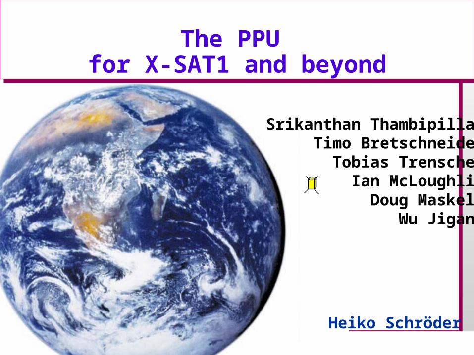
1000 nmRGB 2500 nm
Multispectral
© Heiko Schröder, 2003 Parallel image processing 4
CHRIS
Multispectral
© Heiko Schröder, 2003 Parallel image processing 5
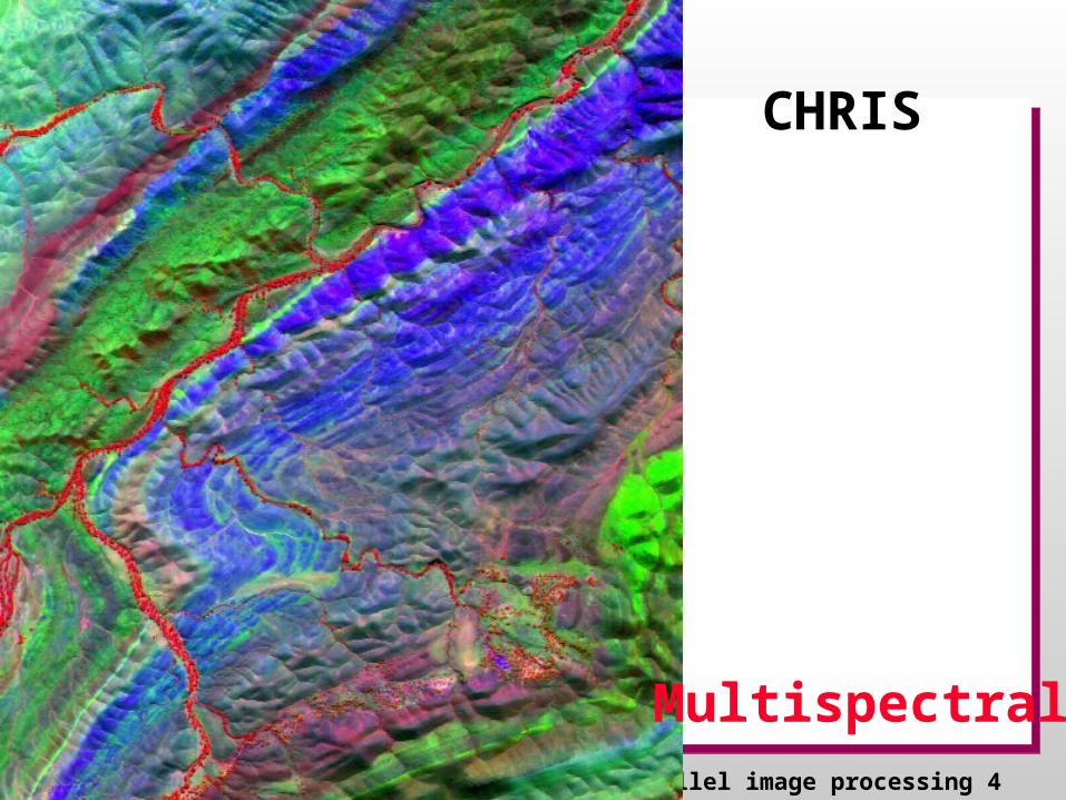
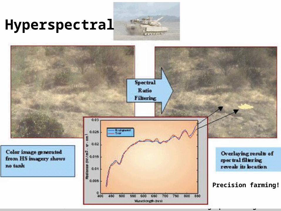
Hyperspectral
Precision farming!

© Heiko Schröder, 2003 Parallel image processing 6
Increasing Performance of X-SAT1Increasing Performance of X-SAT1
7 km/s 100 Mbit/sec 4000 s/orbit 400 Gbit/orbit download: 4 Gbit/orbit
On-board image analysis andcompression
685 km
Singapore100 x output if useful/useless<=1/100
100 x value

© Heiko Schröder, 2003 Parallel image processing 7
Performance evaluation
P=C/A
X-SAT1 without PPU:P=15,000,000/25,000/1200 = .5 $/km2
$12,500 for 50x500 km2 air planeUseful? What are we looking for?
•C -- Cost
•A --image area: Useful (can be sold)

© Heiko Schröder, 2003 Parallel image processing 8
Our aim: High performance via COTS16 processors (+ spares) off-the-shelfconnected via afault tolerant reconfigurable network
Mesh/torus
Real-time

© Heiko Schröder, 2003 Parallel image processing 9
processorsfault
tolerantmesh
on-board
PPU for X-SAT1

© Heiko Schröder, 2003 Parallel image processing 10
FPGA
ctrlh/vo/er/w
Instructionsto PEs
link to PE
BSP?
Mesh with slow recovery
Real-time
© Heiko Schröder, 2003 Parallel image processing 11
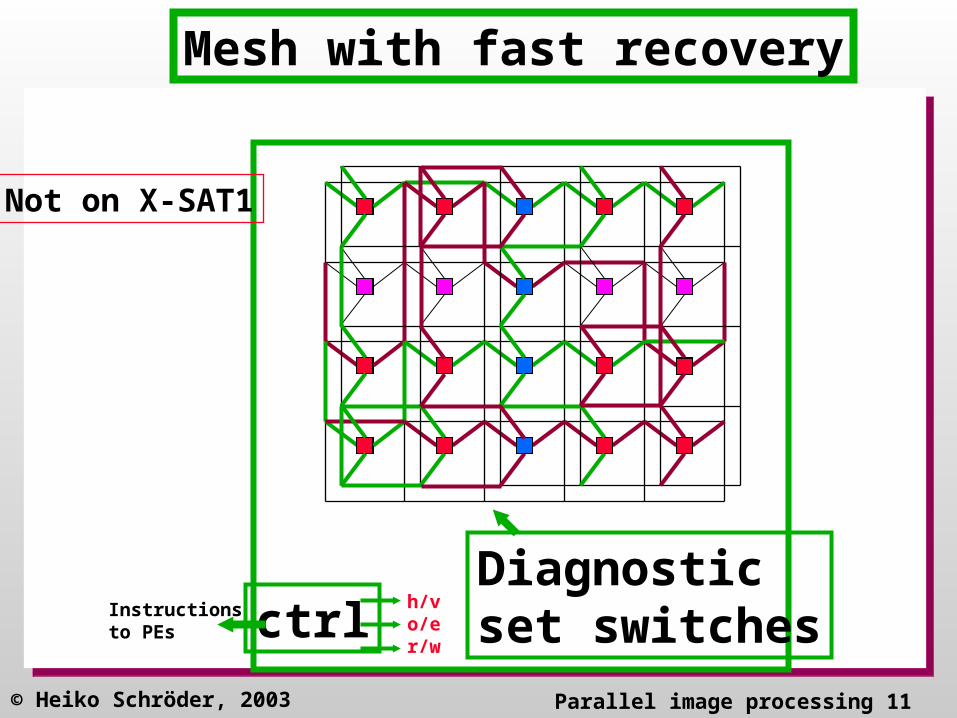
ctrlh/vo/er/w
Instructionsto PEs
Diagnosticset switches
Mesh with fast recovery
Not on X-SAT1
© Heiko Schröder, 2003 Parallel image processing 12
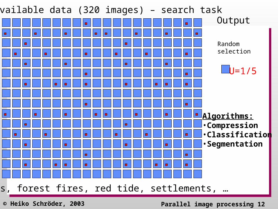
Available data (320 images) – search task
Oil slicks, forest fires, red tide, settlements, …
Randomselection
U=1/5
Output
Algorithms:•Compression•Classification•Segmentation

© Heiko Schröder, 2003 Parallel image processing 13
Compressionratio (CR=4loss-less)
Segmentation gain (SG=16, 1/16 of a useful image is useful)
Classification gain(CG=5, 1 in 5 images contain useful information)
U=.8
U=.2
U=4
U=1 U=16
The satellite efficiency cube
Not likely
LOSSY=60U=32
U=64
(0,0,0)
© Heiko Schröder, 2003 Parallel image processing 14
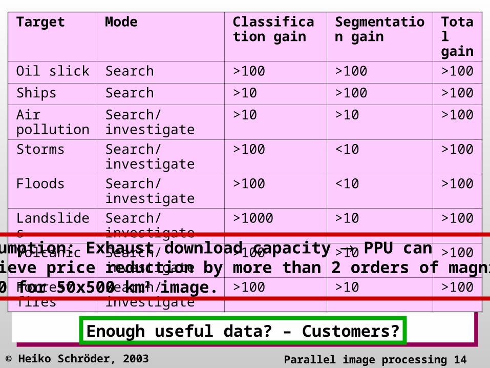
Target Mode Classification gain
Segmentation gain
Total gain
Oil slick Search >100 >100 >100
Ships Search >10 >100 >100
Air pollution Search/investigate >10 >10 >100
Storms Search/investigate >100 <10 >100
Floods Search/investigate >100 <10 >100
Landslides Search/investigate >1000 >10 >100
Volcanic Search/investigate >100 >10 >100
Forrest fires Search/investigate >100 >10 >100
Assumption: Exhaust download capacity PPU can achieve price reduction by more than 2 orders of magnitude$100 for 50x500 km2 image.
Enough useful data? – Customers?
© Heiko Schröder, 2003 Parallel image processing 15
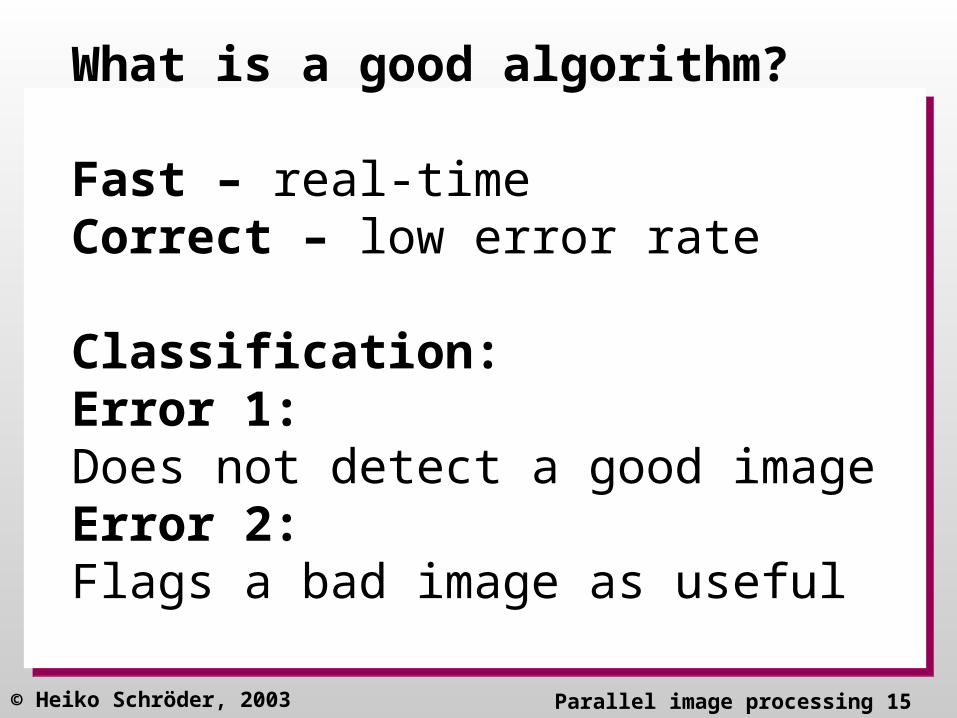
What is a good algorithm?
Fast – real-timeCorrect – low error rate
Classification:Error 1: Does not detect a good imageError 2:Flags a bad image as useful
© Heiko Schröder, 2003 Parallel image processing 16
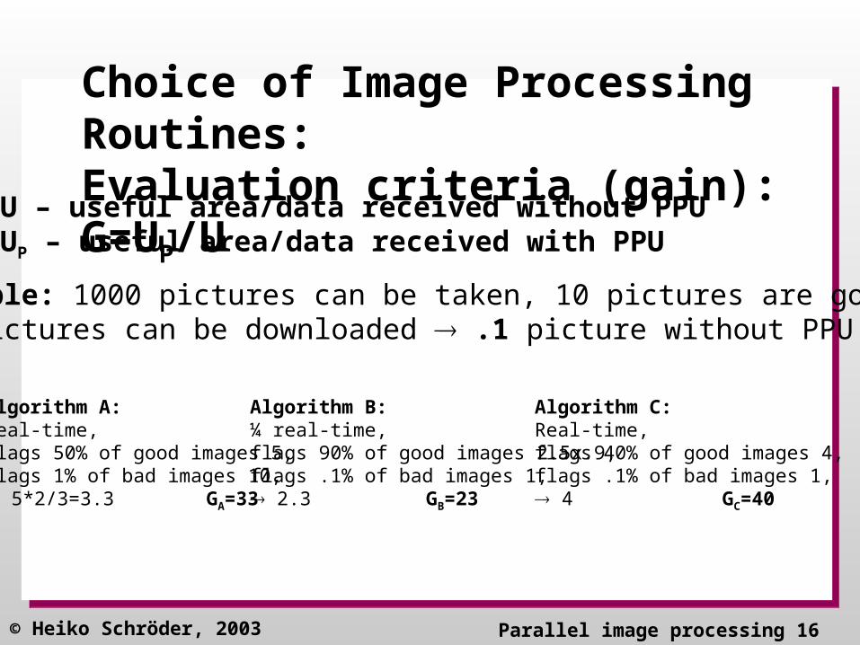
Choice of Image Processing Routines:Evaluation criteria (gain): G=UP/U
U – useful area/data received without PPUUP – useful area/data received with PPU
Algorithm A:Real-time, flags 50% of good images 5, flags 1% of bad images 10, 5*2/3=3.3 GA=33
Example: 1000 pictures can be taken, 10 pictures are good,10 pictures can be downloaded .1 picture without PPU
Algorithm B:¼ real-time, flags 90% of good images 2.5x.9, flags .1% of bad images 1, 2.3 GB=23
Algorithm C:Real-time, flags 40% of good images 4, flags .1% of bad images 1, 4 GC=40

© Heiko Schröder, 2003 Parallel image processing 17
1 2 3 4 5 6 7 8
9 10 11 12 13 14 15 16
17 18 19 20 21 22 23 24
25 26 27 28 29 30 31 32
33 34 35 36 37 38 39 40
41 42 43 44 45 46 47 48
49 50 51 52 53 54 55 56
57 58 59 60 61 62 63 64
LL1+2+3+4
HL1+3-2-4
LH1+2-3-4
HH1+4-2-3
1 2
3 4
LL HL
LH HH
LL HL
LH HH
LL HL
LH HH
LL HL
LH HH
LL HL
LH HH
LL HL
LH HH
LL HL
LH HH
LL HL
LH HH
LL HL
LH HH
LL HL
LH HH
LL HL
LH HH
LL HL
LH HH
LL HL
LH HH
LL HL
LH HH
LL HL
LH HH
LL HL
LH HH
LL LL
LL LL
LL LL
LL LL
LL LL
LL LL
LL LL
LL LL
LH LH
LH LH
LH LH
LH LH
LH LH
LH LH
LH LH
LH LH
HL HL
HL HL
HL HL
HL HL
HL HL
HL HL
HL HL
HL HL
HH HH
HH HH
HH HH
HH HH
HH HH
HH HH
HH HH
HH HH
1 2 3 4 5 6 7 89 10 11 12 13 14 15 16
17 18 19 20 21 22 23 2425 26 27 28 29 30 31 3233 34 35 36 37 38 39 4041 42 43 44 45 46 47 4849 50 51 52 53 54 55 5657 58 59 60 61 62 63 64
L1+2
H1-2
L3+4
H3-4
Invertible!+ /2 - /2

© Heiko Schröder, 2003 Parallel image processing 18
HL1 HL1 HL1 HL1
HL1 HL1 HL1 HL1
HL1 HL1 HL1 HL1
HL1 HL1 HL1 HL1
HH1HH1HH1HH1
HH1HH1HH1HH1
HH1HH1HH1HH1
HH1HH1HH1HH1
LH1 LH1 LH1 LH1
LH1 LH1 LH1 LH1
LH1 LH1 LH1 LH1
LH1 LH1 LH1 LH1
LL1 LL1 LL1 LL1
LL1 LL1 LL1 LL1
LL1 LL1 LL1 LL1
LL1 LL1 LL1 LL1
7+8+15+16
23+24+31+32
38+40+47+48
55+56+63+64
5+6+13+14
21+22+29+30
37+38+24+46
53+54+61+62
3+4+11+12
19+20+27+28
35+36+43+44
51+52+59+60
1+2+9+10
17+18+25+26
33+34+41+42
49+50+57+58
LL2
LH2
LH2
LH2
LH2
HL2
HL2
HH2
HH2
HL2
HL2
HH2
HH2
LL2
LL2 LL2LH3
HL3
HH3
LL3
33+42-34-41
35+44-36-43
49+58-50-57
51+60-52-59
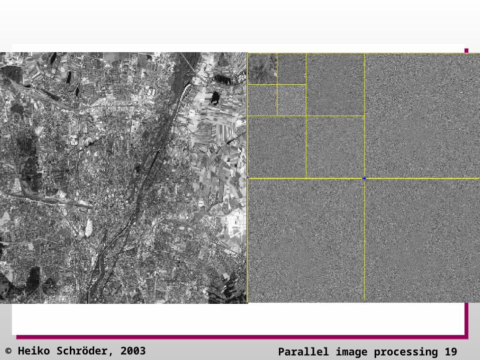
© Heiko Schröder, 2003 Parallel image processing 19
© Heiko Schröder, 2003 Parallel image processing 20
How to find areas of interestImage classification
?

© Heiko Schröder, 2003 Parallel image processing 21
Thresholding

© Heiko Schröder, 2003 Parallel image processing 22
Mathematical morphologyMathematical morphology
erosion
dilation
erosion
edge detection, thinning, noise removal, enlarging
Structural elementreference point

© Heiko Schröder, 2003 Parallel image processing 23
ThresholdingMM-segmentation

© Heiko Schröder, 2003 Parallel image processing 24
MM-Hough TransformMM-Hough Transform
reference pointerosion
m d
d
m
a dot leads to one addition if there is a matching point

© Heiko Schröder, 2003 Parallel image processing 25
1min420km
Investigative mode
72 sec500km
36sec250km

© Heiko Schröder, 2003 Parallel image processing 26
30 sec210km
7 min2900 km Follow coast
Search mode
400 sec:Storm: 3kmShip: 5kmFire: 50mAir plane: 100km

© Heiko Schröder, 2003 Parallel image processing 27
2000 km
High-performance Computer network
Image analysis•Classification•Segmentation•compression
Intelligent search
Maximize the efficiency/useful outputof the satellite!
200 km

© Heiko Schröder, 2003 Parallel image processing 28
skeletonsskeletons
Compression and classification
© Heiko Schröder, 2003 Parallel image processing 29
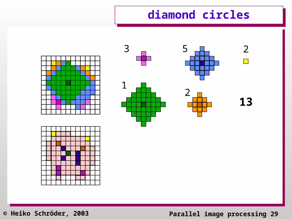
diamond circlesdiamond circles
23
21
5
13

© Heiko Schröder, 2003 Parallel image processing 30
odd square circlesodd square circles
• 8-neighbourhood skeleton
3 6
13
0 4

© Heiko Schröder, 2003 Parallel image processing 31
square circlessquare circles
• red-square-skeleton
1
1
0
3
0
0
0
1
6
© Heiko Schröder, 2003 Parallel image processing 32
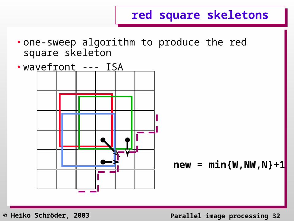
red square skeletonsred square skeletons
• one-sweep algorithm to produce the red square skeleton
• wavefront --- ISA
new = min{W,NW,N}+1

© Heiko Schröder, 2003 Parallel image processing 33
granularitygranularity
• Histograms of skeletons classify images
© Heiko Schröder, 2003 Parallel image processing 34
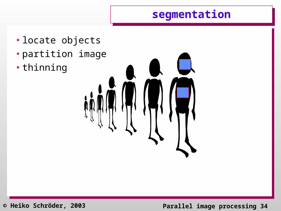
segmentationsegmentation
• locate objects
• partition image
• thinning

© Heiko Schröder, 2003 Parallel image processing 35
Mathematical morphologyMathematical morphology
erosion
dilation
erosion
edge detection, thinning, noise removal, enlarging
Structural elementreference point

© Heiko Schröder, 2003 Parallel image processing 36
Border followingBorder following
X1 2
356
78
4 2 3 3 3 3 3 345
655
66
678
81
8111
Image classification1 2 3 4 5 6 7 8
Histogram:
#

© Heiko Schröder, 2003 Parallel image processing 37
Image classification IImage classification I

© Heiko Schröder, 2003 Parallel image processing 38
Image classification IIImage classification II
© Heiko Schröder, 2003 Parallel image processing 39
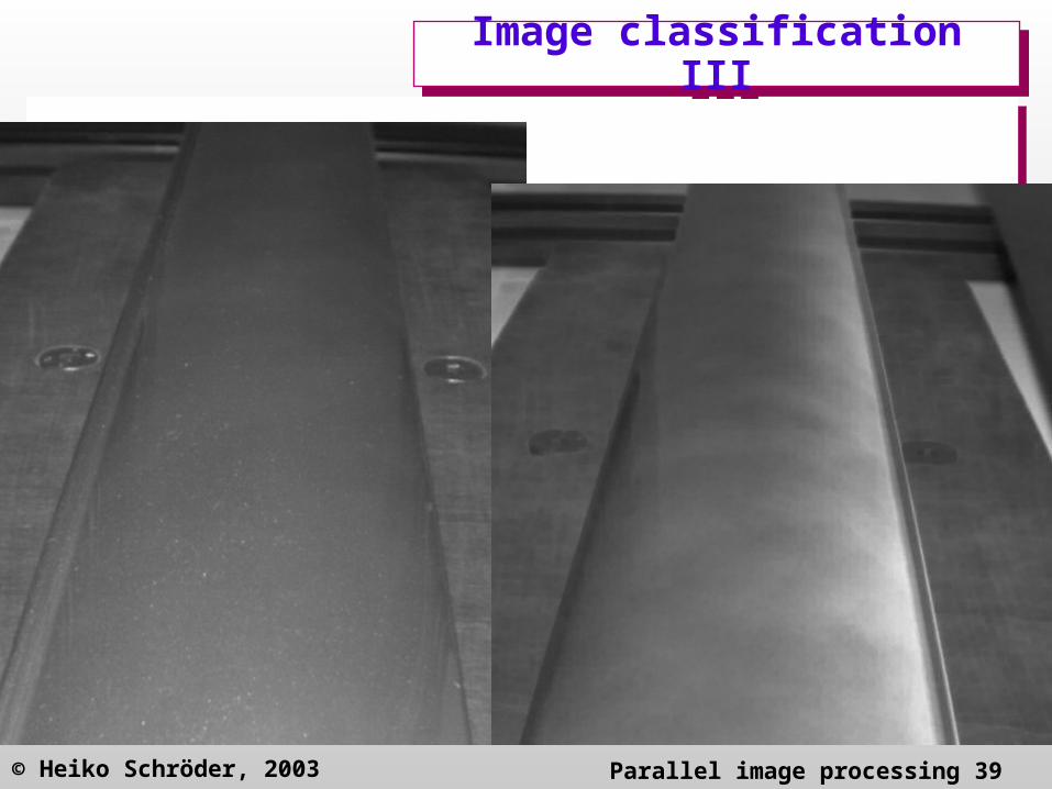
Image classification IIIImage classification III

© Heiko Schröder, 2003 Parallel image processing 40
Hough transformHough transform
• good line detection method
m d
d
m
every dot leads to M (1K) additions
d
m

© Heiko Schröder, 2003 Parallel image processing 41
MM-Hough transformMM-Hough transform
reference pointerosion
m d
d
m
a dot leads to one addition if there is a matching point

© Heiko Schröder, 2003 Parallel image processing 42
HT on the ISAHT on the ISA
Bertil

© Heiko Schröder, 2003 Parallel image processing 43
shearingshearing
0
1
2
3
4
5 column sum
15/2022/10
MMOR
OR
AND
15/25/6 12/28/16
eliminates dirt
OR
AND
15/10 12/16
d
d : parameter
© Heiko Schröder, 2003 Parallel image processing 44
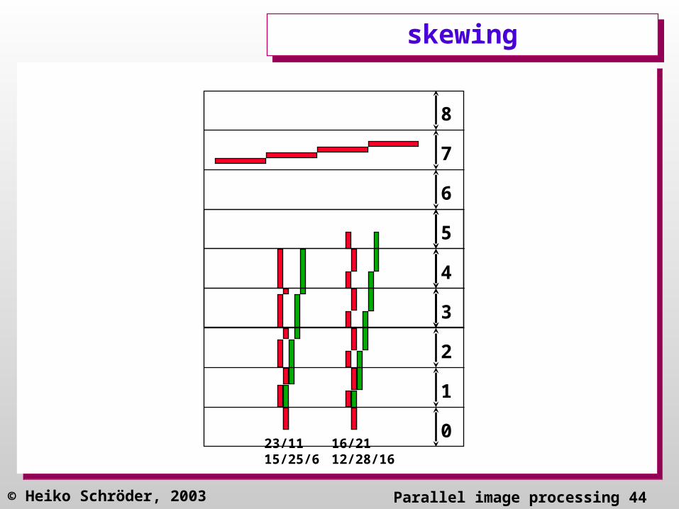
skewingskewing
0
1
2
3
4
5
6
7
8
23/1115/25/6
16/2112/28/16

© Heiko Schröder, 2003 Parallel image processing 45
alternativesalternatives
0
1
2
3
4
5
6
7
8
MM
OR
OR
OR
AND
AND
}}
OR}
OR
OR
OR
AND
AND
}}
OR}

© Heiko Schröder, 2003 Parallel image processing 46
advantages of MM-HTadvantages of MM-HT
• higher contrast
• less additions
• more flexibility– lines of given thickness
– dashed lines
– lines of given length
– lines of given orientation
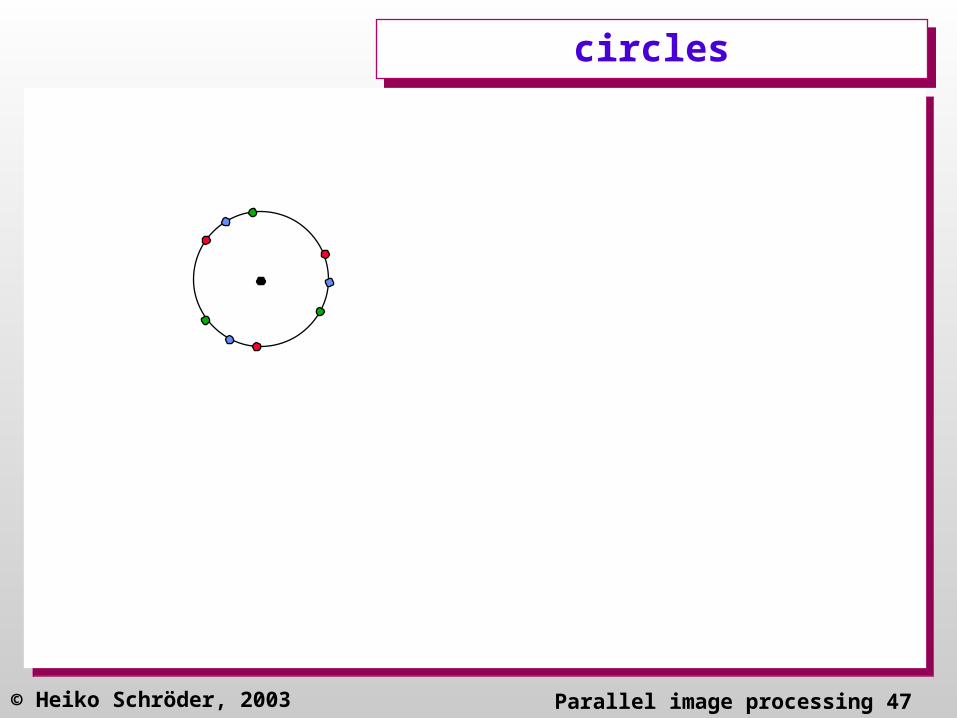
– circles, …
• tomography !!
© Heiko Schröder, 2003 Parallel image processing 47
circlescircles

© Heiko Schröder, 2003 Parallel image processing 48
Hough transform IHough transform I

© Heiko Schröder, 2003 Parallel image processing 49
Hough transform IIHough transform II

© Heiko Schröder, 2003 Parallel image processing 50
robot visionrobot vision
projectorCCD CCD
• stereo vision
thinning (skeletons or erosion), line detection (MM-HT), trigonometry


© Heiko Schröder, 2003 Parallel image processing 52
Design a mathematical morphology algorithm (and demonstrate by means of example), that removes all isolated patterns of size 2 (black black on white and white on black). It does not change any set of 3 neighbouring pixels with identical colour.
Write an algorithm that removes all squares of maximal size from a given image.
Write a program based on MM, that fills gaps in horizontal and vertical lines up to length 2, but does not prolong the ends of lines.

Application specific massive parallelism
Application specific massive parallelism
Low cost alternatives to polygons for visualisation

© Heiko Schröder, 2003 Parallel image processing 54
contentscontents
•scan-line image processing
•PIPS architecture
•from landscapes to 3D
•surface generation for CAD

© Heiko Schröder, 2003 Parallel image processing 55
basic architecturebasic architecture
1
1024
highresolutionreal time

© Heiko Schröder, 2003 Parallel image processing 56
PIPS (1990-94)PIPS (1990-94)
1 M bit
1 M bit
32x32 torus16 bit parallelcommunication16 bit addprefetch
memory control
BHP -- CSIRO -- NU -- ADFA 1.4 M
© Heiko Schröder, 2003 Parallel image processing 57
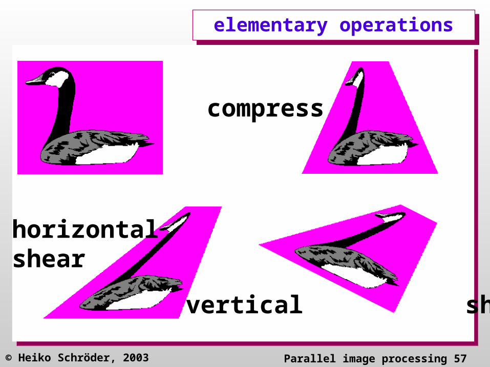
elementary operationselementary operations
compress
horizontalshear
vertical shear
© Heiko Schröder, 2003 Parallel image processing 58
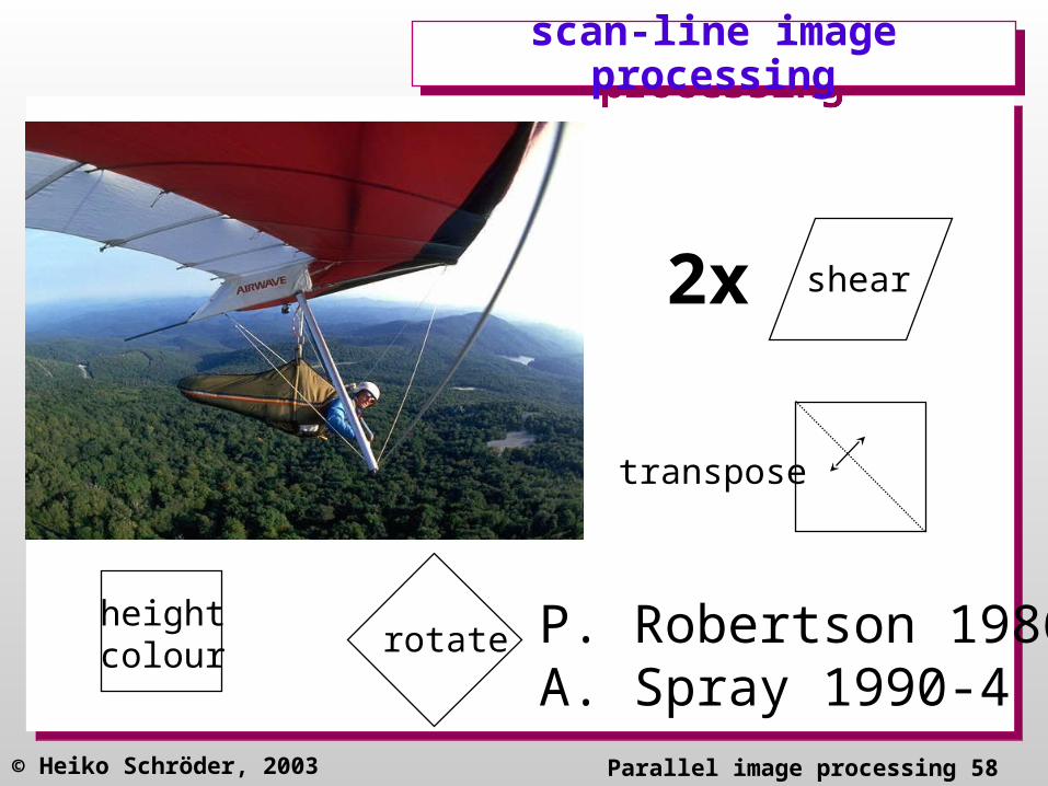
scan-line image processingscan-line image processing
heightcolour rotate
shear2x
transpose
P. Robertson 1986A. Spray 1990-4
© Heiko Schröder, 2003 Parallel image processing 59
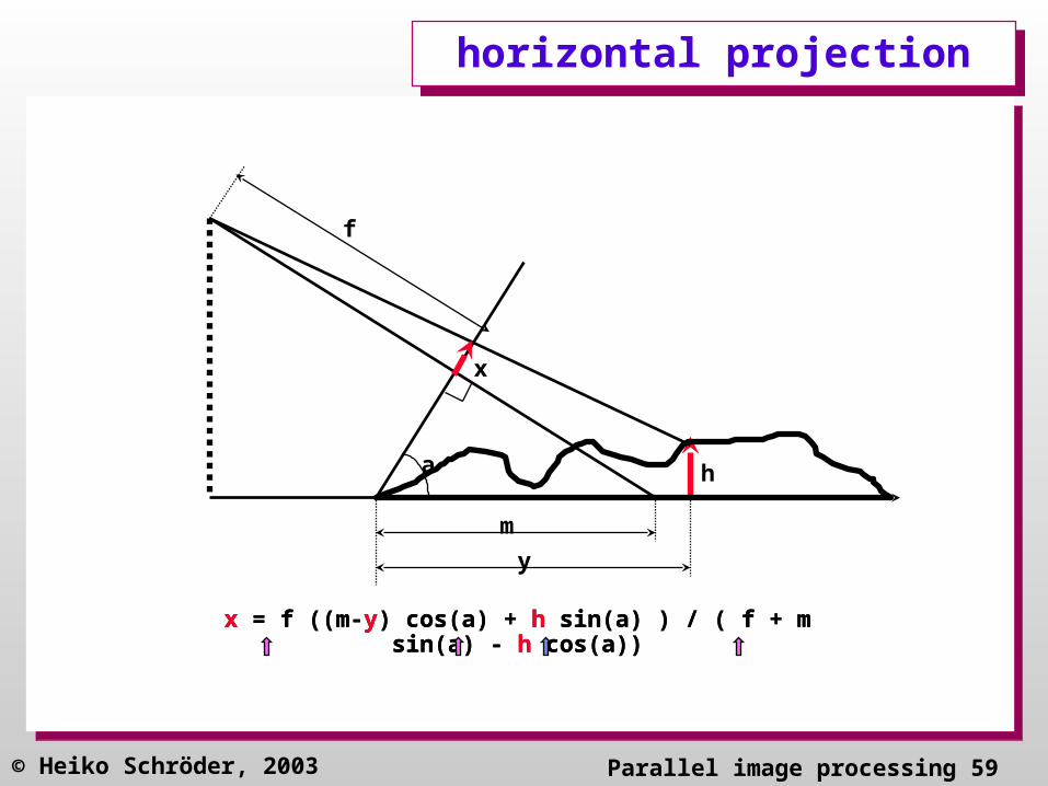
horizontal projectionhorizontal projection
f
h
m
y
a
x
x = f ((m-y) cos(a) + h sin(a) ) / ( f + m sin(a) - h cos(a))x = f ((m-y) cos(a) + h sin(a) ) / ( f + m sin(a) - h cos(a))
© Heiko Schröder, 2003 Parallel image processing 60
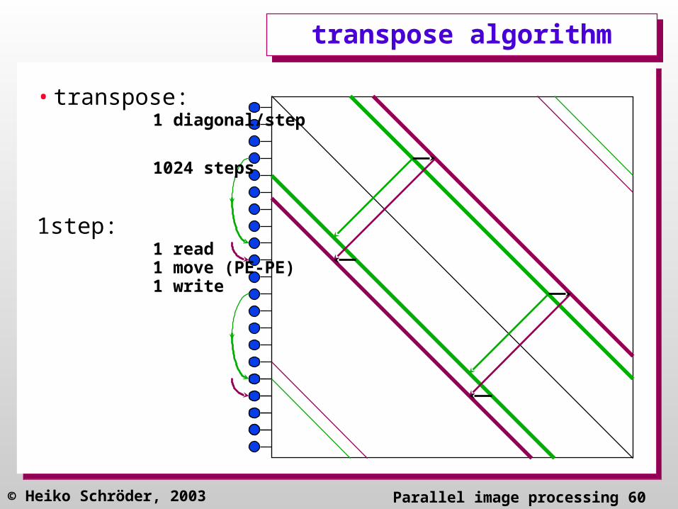
transpose algorithmtranspose algorithm
• transpose:1 diagonal/step
1024 steps
1step:1 read1 move (PE-PE)1 write

© Heiko Schröder, 2003 Parallel image processing 61
HC/torus diameter / bandwidth
HC/torus diameter / bandwidth
1024 nodes
12
Diameter 32
56
Diameter 10
56*4= 22412*16=192
4 bit wide
16 bit wide
© Heiko Schröder, 2003 Parallel image processing 62
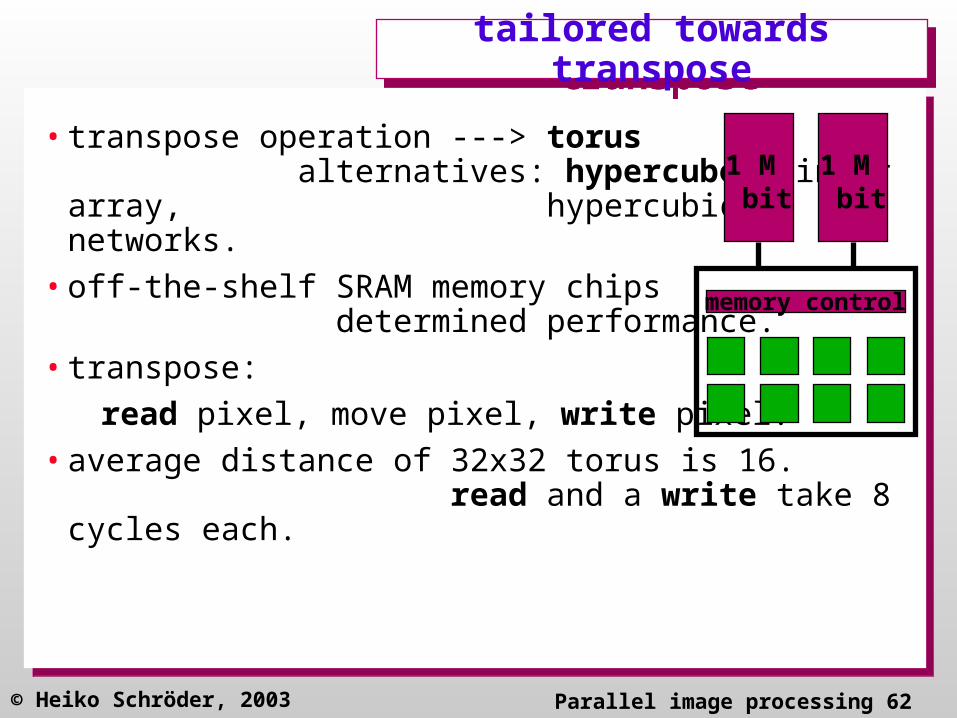
tailored towards transposetailored towards transpose
• transpose operation ---> torus alternatives: hypercube, linear array, hypercubic networks.
• off-the-shelf SRAM memory chips determined performance.
• transpose:
read pixel, move pixel, write pixel.
• average distance of 32x32 torus is 16. read and a write take 8 cycles each.
1 M bit
1 M bit
memory control
© Heiko Schröder, 2003 Parallel image processing 63
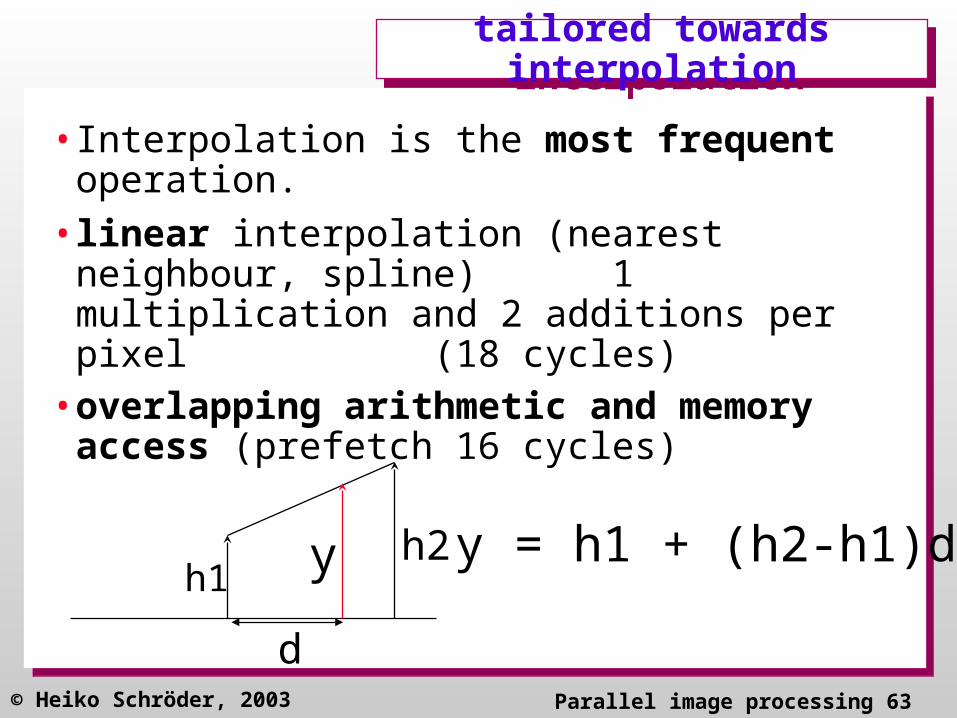
tailored towards interpolationtailored towards interpolation
• Interpolation is the most frequent operation.
• linear interpolation (nearest neighbour, spline) 1 multiplication and 2 additions per pixel (18 cycles)
• overlapping arithmetic and memory access (prefetch 16 cycles)
yh1h2
d
y = h1 + (h2-h1)d

© Heiko Schröder, 2003 Parallel image processing 64
performanceperformance
• 1 perspective view (464 K)– 1 rotation (170 K)
3 shears (3x36 K) 2 transpose (2x 31 K)
– 1 compress (41 K)
– 1 projection (219 K)
– 1 image output (34 K)
• 464 K x 50ns = 23.2 ms
• 43 frames / sec

© Heiko Schröder, 2003 Parallel image processing 65
performance parametersperformance parameters
• 20 GOPS (16 bit words)
• IEEE standard 32bit floating point:– 200 instructions / floating point operation
– 100 MFLOPS / 1024 PEs
• fast floating point:– 80 instructions / floating point operation
– 250 MFLOPS / 1024 PEs
• 5 Gbytes/s internal memory bandwidth
• 40 Gbytes/s inter-processor communication

© Heiko Schröder, 2003 Parallel image processing 66
performanceperformance
Main criterion: high throughput
machine A: price PA, time k tB
machine B: price k PA, time tB
k A-machines cost and produceas much as one B-machine
evaluation criterion: Cost x time(cost x period; AT; AP)

© Heiko Schröder, 2003 Parallel image processing 67
cost-performancecost-performance
Time cost cost x Time
SUN 2 min 3 K 360
MasPar 5 sec 100 K 5001024
PIPS 1/40 sec 20 K 1/21024
© Heiko Schröder, 2003 Parallel image processing 68
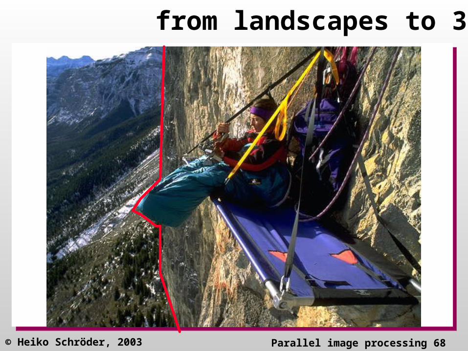
from landscapes to 3D

© Heiko Schröder, 2003 Parallel image processing 69
Unsolved problems:•partitioning 3D surfaces into landscapes•detail on demand•target architecture (distributed & parallel)•...

© Heiko Schröder, 2003 Parallel image processing 70
partitioning the surfaces
into pieces of landscapes
Bez, May, Schroeder

© Heiko Schröder, 2003 Parallel image processing 71
partitioning algorithmspartitioning algorithms
• fixed set of observer points?
• how many?
• observer position data dependent?

© Heiko Schröder, 2003 Parallel image processing 72
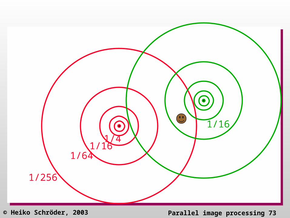
Detail on demandDetail on demand
1/4
1/161/64
1/256
1/1
© Heiko Schröder, 2003 Parallel image processing 73
1/161/64
1/256
1/4
1/16

© Heiko Schröder, 2003 Parallel image processing 74
Levels of resolutionLevels of resolution
Provide image at various levels of resolution
3
4
411
1
,...2,1,0,4
1
i
ii
a
ia

© Heiko Schröder, 2003 Parallel image processing 75
detail on demanddetail on demand
wavelet transform ?•all data should be kept at several levels of resolution
R. Lang, P. Lenders, H. Schroeder (1995/6)

© Heiko Schröder, 2003 Parallel image processing 76
Wavelet transform (simplified)
Wavelet transform (simplified)
113
1211
ad
dd
223
2221
ad
dd
333
3231
ad
dd
443
4241
ad
dd
Easy reconstruction!
3
14
3,2,1,
kikii
ijiij
dax
jdax
ij
i
d
a Low-pass-filter
High-pass-filter

© Heiko Schröder, 2003 Parallel image processing 77
Spiral (Rein Warmels)Spiral (Rein Warmels)

© Heiko Schröder, 2003 Parallel image processing 78
Butterfly network for FFTButterfly network for FFT
FFTfrequency spectrumimage classification
CM2

© Heiko Schröder, 2003 Parallel image processing 79
FFT without butterflyFFT without butterfly
3 5 7 9 11 13 152 4 6 8 10 12 14 161
1 2 5 6 9 10 13 143 4 7 8 11 12 15 16
1 3 2 4 9 11 10 125 7 6 8 13 15 14 16
1 5 3 7 2 6 4 89 13 11 15 10 14 12 16
© Heiko Schröder, 2003 Parallel image processing 80
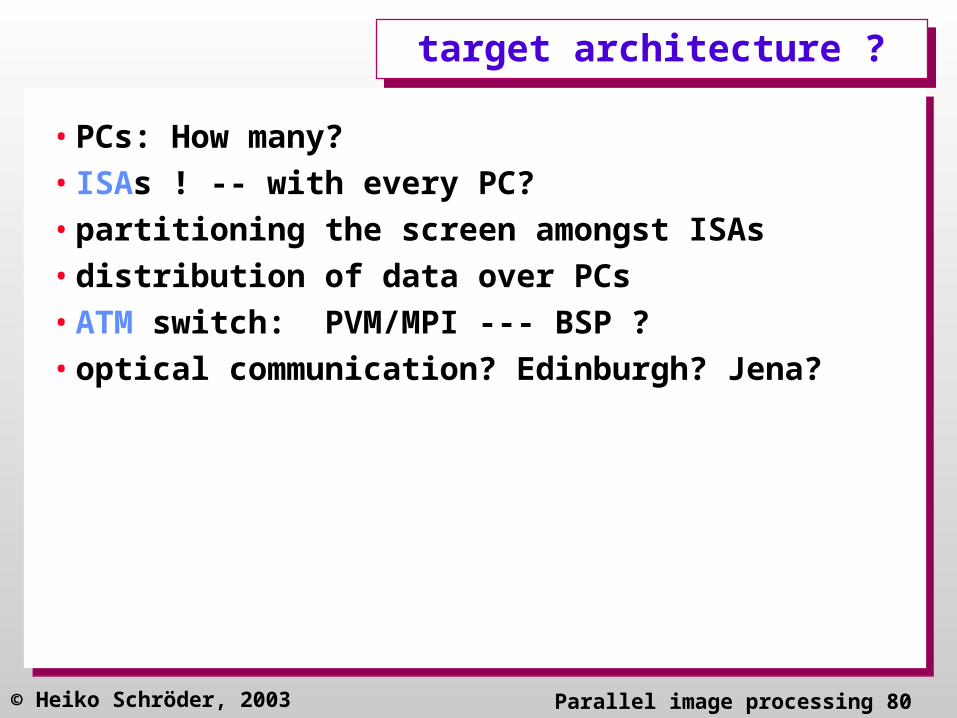
target architecture ?target architecture ?
• PCs: How many?
• ISAs ! -- with every PC?
• partitioning the screen amongst ISAs
• distribution of data over PCs
• ATM switch: PVM/MPI --- BSP ?
• optical communication? Edinburgh? Jena?
© Heiko Schröder, 2003 Parallel image processing 81
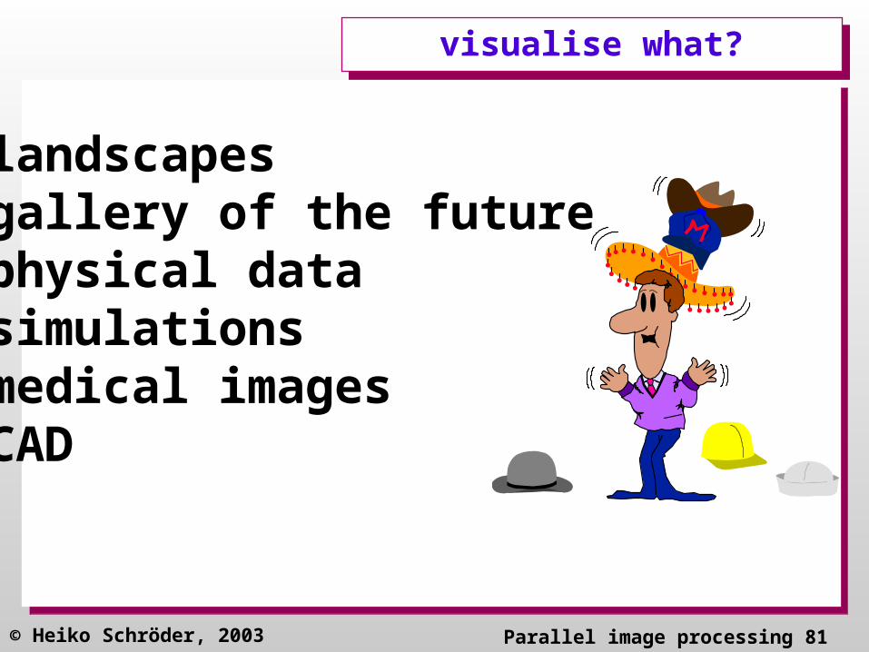
visualise what?visualise what?
•landscapes •gallery of the future •physical data•simulations•medical images•CAD
© Heiko Schröder, 2003 Parallel image processing 82
++
+ +
+
+ + +
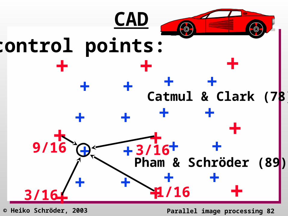
+control points:
+
+ +
+ +
+ +
+
+
+ +
+ +
+ +
+
CAD
9/16 3/16
3/16 1/16
Catmul & Clark (78)
Pham & Schröder (89)

© Heiko Schröder, 2003 Parallel image processing 83
+ +
++
(9A + 3C + 3D + B)/16
C
B
D
A
9 add-shift 9/4 per control point3 per pixel +

© Heiko Schröder, 2003 Parallel image processing 84
move algorithms ?move algorithms ?
•routing algorithm (warping)?–hot potato? (Kaufmann, Schröder 94)
•warping “cheaper” than general routing?

© Heiko Schröder, 2003 Parallel image processing 85
scan-lines ?scan-lines ?
• tiling? -- no transpose!
•hidden surface removal via “z”-value

low cost, real-time,high resolution visualisation
can be done !!!