Hedge Fund Strategies, Performance, Risk and Disasters and their Prevention

William T. Ziemba

Sauder School of Business, UBC

Vancouver, BC

EUMOptFin3 Workshop

Bergamo, Italy

May 17-21, 2004

It is clear that hedge funds got into trouble by overbetting and not being truly diversified, and vulnerable, they then got caught by low probability but plausible disaster scenarios that occurred.

It is exactly then - when you are in trouble - that you need access to new cash and since that is usually not available, it makes more sense to plan ahead for such contingencies by not overbetting and by being truly diversified in advance.

• Hedge funds are pooled investments that attempt to obtain superior returns for their mostly wealthy investors.

• The name hedge fund is misleading since it is a vehicle to trade a pool of money from a number of investors in various financial markets.

• The general partner runs the fund and collects fees to compensate for expenses and receives bonuses for superior performance.

• Typically, the general partner is an investor in the fund.

• This is called eating your own cooking.

• It gives investors added confidence and increases the incentive for the manager to perform well and dampens the incentive of the manager to take excessive risks.

• The latter is especially important since operating a hedge fund is essentially a call option on the investor's wealth.

• In addition it is convenient for the general partner to store fees collected month by month or quarter by quarter in the fund.

• In the last two decades, the hedge fund industry has grown explosively. The first official hedge fund was established in 1949.

• By the late 1980’s, the number of funds had increased to about 100. In 1997 there were more than 1200 hedge funds, managing a total of more than $200 billion.

• Currently, hedge funds have over $600 billion in assets.

• Though the number and size of hedge funds are still small compared to mutual fund industry, their growth reflects the importance of alternative investments for institutional investors and wealthy individuals.

• Hedge funds frequently exert an influence on financial markets that is much greater than their size.

• Fixed Income Arbitrage - long and short bond positions via cash or derivatives markets in government, corporate and/or asset-backed securities. The risk varies depending on duration, credit exposure and the degree of leverage.

• Event Driven - a strategy that attempts to benefit from mispricing arising in different events such as merger arbitrage, restructurings, etc. Positions are taken in undervalued securities anticipated to rise in value due to events such as mergers, reorganizations, or takeovers. The main risk is non-realization of the event.

• Equity Convergence Hedge – investing in equity or equity derivative instruments whose net exposure (gross long minus short) is low. The manager may invest globally, or have a more defined geographic, industry or capitalization focus. The risk primarily pertains to the specific risk of the long and short positions.

• Restructuring – buying and occasionally shorting securities of companies under Chapter 11 and/or ones which are undergoing some form of reorganization. The securities range from senior secured debt to common stock. The liquidation of financially distressed companies is the main source of risk.

• Event Arbitrage – purchasing securities of a company being acquired and shorting the acquiring company. This risk relates to the “deal” risk rather than market risk.

• Capital Structure Arbitrage -buying and selling different securities of the same issuer (e.g.convertibles/common stock) attempting to obtain low volatility returns by exploiting the relative mispricing of these securities.

Market Neutral Strategies

• Macro - an attempt to capitalize on country, regional and/or economic change affecting securities, commodities, interest rates and currency rates. Asset allocation can be aggressive, using leverage and derivatives. The method and degree of hedging can vary significantly.

• Long – a “growth”, “value”, or other model approach to investing in equities with no shorting or hedging to minimize market risk. These funds mainly invest in emerging markets where there may be restrictions on short sales.

• Long Bias – similar to equity convergence but a net long exposure.

• Short – selling short over-valued securities attempting to repurchasing them in the future at a lower price.

Directional Strategies

If you bet on a horse, that’s gambling. If you bet you can make three spades, that’s entert ainment. If you bet cotton will go up three points, that’s b usiness. See the difference?

Blackie Sherrod

Unbridled at Claiborne Farms, Paris, Kentucky

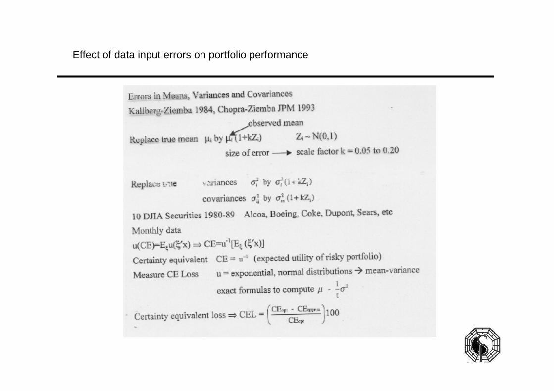
Effect of data input errors on portfolio performance

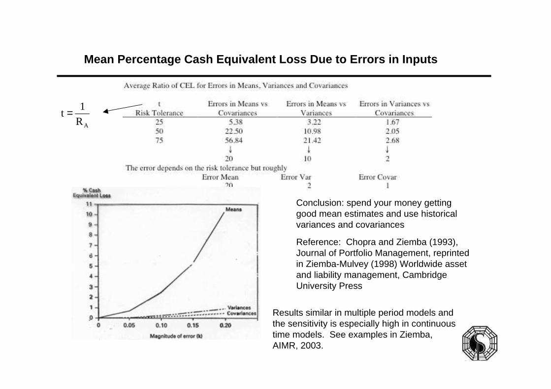
Mean Percentage Cash Equivalent Loss Due to Errors i n Inputs

Conclusion: spend your money getting good mean estimates and use historical variances and covariances

Reference: Chopra and Ziemba (1993), Journal of Portfolio Management, reprinted in Ziemba-Mulvey (1998) Worldwide asset and liability management, Cambridge University Press

Results similar in multiple period models and the sensitivity is especially high in continuous time models. See examples in Ziemba, AIMR, 2003.

t = 1

RA

• Unofficial, that is private, hedge funds have been run for centuries using futures, equities and other financial instruments.

• Futures in rice trading in Japan date from the 1700s and futures trading in Chicago was active in the mid 1800s.

• An interesting early hedge fund was the Chest Fund at King's College, Cambridge which was managed by the First Bursar who was the famous economic theorist John Maynard Keynes from 1927 to 1945.

• In November 1919 Keynes was appointed second bursar.

• Up to this time King's College investments were only in fixed income trustee securities plus their own land and buildings.

• By June 1920 Keynes convinced the college to start a separate fund containing stocks, currency and commodity futures.

• Keynes became first bursar in 1924 and held this post which had final authority on investment decisions until his death in 1945.

Keynes as a hedge fund manager

Keynes emphasized three principles of successful investments in his 1933 report

(1) a careful selection of a few investments (or a few types of investment) having regard to their cheapness in relation to their probable actual and potential intrinsic value over a period of years ahead and in relation to alternative investments at the time;

(2) a steadfast holding of these in fairly large units through thick and thin, perhaps for several years,until either they have fullfilled their promise or it is evident that they were purchased on a mistake;

(3) a balanced investment position, i.e., a variety of risks in spite of individual holdings being large, and if possible, opposed risks.

Keynes did not believe in market timing.

We have not proved able to take much advantage of a general systematic movement out of and into ordinary shares as a whole at different phases of the trade cycle … As a result of these experiences I am clear that the idea of wholesale shifts is for various reasons impracticable and indeed undesirable. Most of those who attempt to sell too late and buy too late, and do both too often, incurring heavy expenses and developing too unsettled and speculative a state of mind, which, if it is widespread, has besides the grave social disadvantage of aggravating the scale of the fluctuations.

Keynes' ideas overlap to some extent with Warren Buffett's Berkshire Hathaway fund with an emphasis on value, large holdings, and patience.

Buffett also added great involvement in the management of his holdings plus very effective side businesses such as insurance. Keynes' approach of a small number of positions even partially hedged naturally leads to fairly high volatility as shown in his aggregate yearly performance given in the Table and Figure.

Details of the holdings over time, as with hedge funds, are not known, but is is known that in 1937 the fund had 130 separate positions.

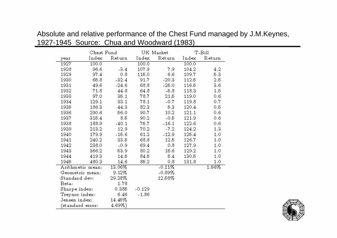
Absolute and relative performance of the Chest Fund managed by J.M.Keynes, 1927-1945 Source: Chua and Woodward (1983)

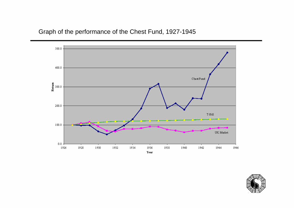
Graph of the performance of the Chest Fund, 1927-1945

•These returns do not include dividends and interest.

•This income, which is not public information, was spent on modernizing and refurbishing King's College.

• The index's dividend yield was under 3%.

• A CAPM analysis suggests that Keynes was an aggressive investor with a beta of 1.78 versus the benchmark United Kingdom market return, a Sharpe ratio of 0.385, geometric mean returns of 9.12% per year versus -0.89% for the benchmark.

•Keynes had a yearly standard deviation of 29.28% versus 12.55% for the benchmark.

•The drawdown from 100 in 1927 to 49.6 in 1931 with losses of 32.4% in 1930 and 24.6% in 1931 was more than 50% but this was during the depression when the index fell 20.3% and 25.0%, respectively.

•The College's patience with Keynes was rewarded in the substantial rise in the Fund during 1932-37 to 315.4.

•Keynes' aggressive approach caught up with him as Britain prepared for World War II in 1938-40 with his index falling to 179.9. Then, during the actual war, 1941-45, Keynes had a strong record.

•In summary, Keynes' turning 100 into 480.3 in 18 years, versus 85.2 for the index, plus dividends and interest given to the College gives Keynes' a good record as a hedge fund manager.

•Keynes' aggressive style, which is similar to Kelly betting, leads to great returns and losses and embarrassments.

•Not covering a grain contract in time led to Keynes taking delivery and filling up the famous Kings' College chapel.

• Fortunately the chapel was big enough to fit in the grain and store it safely until it could be sold.

•The Sharpe ratios and CAPM results are based on normality and a better way to calculate Keynes' β's is through is through Leland's (1999)} B's (discussed in Ziemba, 2003) which applies for the fat tails that Keynes had.

•Keynes' aggressive style is close to log utility so a γ of 1.25 approximates his behavior which compares to 1/γ=80% in the log optimal portfolio and 20% in cash.

• I have been fortunate to work and consult with four individuals who used investment market anomalies and imperfections and hedge funds ideas to turn a humble beginning with essentially zero wealth into hundreds of millions.

• Each had several common characteristics: a gambling background obtained by playing blackjack professionally and a very focused, fully researched and computerized system for asset position selection and careful attention to the possibility of loss.

• Each of these individuals focused more on not losing rather than winning.

• Two were relative value long/short managers eaking out small edges consistently.

• One was a futures trader taking bets on a large number of liquid financial assets based on favorable trends (interest rates, bonds and currencies were the best).

• The fourth was a Hong Kong horse race bettor.

• Their gambling backgrounds led them to conservative investment behavior and excellent results both absolute and risk adjusted.

• They have their losses but rarely do they overbet or non-diversify enough to have a major blow out like the hedge fund occurrences.

• Good systems for diversification and bet size.

Gamblers as hedge fund managers

• Dr.Edward O. Thorp, a mathematician with a PhD from UCLA, became famous in 1960 after devising a simple to use card counting system for beating the card game blackjack.

• In 1966 Thorp wrote a follow-up to his 1962 Beat the Dealer called Beat the Marketwhich outlined a system for obtaining edges in warrant markets.

• Thorp was close to finding the Black Scholes formula for pricing options at least from an approximate, empirical and discrete time point of view and some of these ideas were obviously used in his hedge fund, Princeton Newport Partners (PNP) trading.

• Thorp wrote the foreword to my book with Donald Hausch, Beat the Racetrack published in 1984 which provided a simple to use winning system for racetrack betting based on weak market inefficiencies in the more complex place and show markets using probabilities estimated from the simpler win market.

• The PNP hedge fund, with offices in Newport Beach, California and Princeton, New Jersey, was run from 1969 to 1988 using a variety of strategies, many of which can be classified as convergence or long-short.

• Actual trades and positions used by Thorp and his colleagues are not public information, but a Nikkei put warrant risk arbitrage trade that Thorp and I jointly executed based on my ideas discussed in below gleans some idea of the approach used.

• The basic idea is to sell $A$ at an expensive price, hedge it with the much cheaper close substitute A’, then wait until the prices converge and cash out and remember to not overbet.

Ed Thorp

NSA puts and calls NSA puts and calls on the Toronto and American stock exchanges, 1989-1992

The various NSA puts and calls were of three basic types. Let NSA0 be today's NSA and E0be today's exchange rate. Then Ee is the strike price and NSAe be the exchange rate on expiry for Canadian or US dollars into yen. The symbol (X)+ means the greater of X or zero.

Our convergence trades in late 1989 to early 1990 involved:

1. selling expensive Canadian currency Bankers Trust I's and II's and buying cheaper US currency BT's on the American Stock Exchange; and

2. selling expensive Kingdom of Denmark and Saloman I puts on the ASE and buying the same BT I's also on the ASE both in US dollars. This convergence trade was especially interesting because the price discrepancy was based mainly on the unit size.

We performed a complex pricing of all the warrants which is useful in the optimization of the positions size, see Shaw, Thorp and Ziemba (1995).

However, the Table gives insight into this in a simple way. For example, 9.8% premium year year means that if you buy the option, the NSA must fall 9.8% each year to break even.

So selling at 9.8% and buying 2.6% looks like a good trade. A stochastic programming optimization model helps in determining how much to sell give the risks and your wealth level.

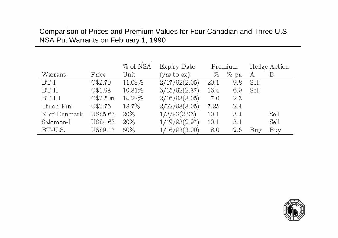
Comparison of Prices and Premium Values for Four Canadian and Three U.S. NSA Put Warrants on February 1, 1990

• Large price discrepancy across Canadian/U.S. border

• Canadians trade in Canada, US's trade in U.S

• Different credit risk

• Different currency risk

• Difficulties with borrowing for short sales

• Blind emotions vs reality

• An inability of speculators to properly price the warrants

Some of the reasons for the different prices were:

The market was confused; % unit became important

BT U.S. cheapest even though its nominal price was highest.

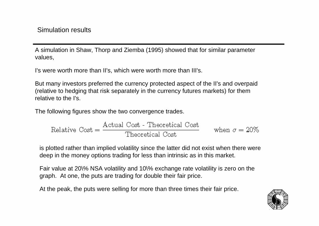
A simulation in Shaw, Thorp and Ziemba (1995) showed that for similar parameter values,

I's were worth more than II's, which were worth more than III's.

But many investors preferred the currency protected aspect of the II's and overpaid (relative to hedging that risk separately in the currency futures markets) for them relative to the I's.

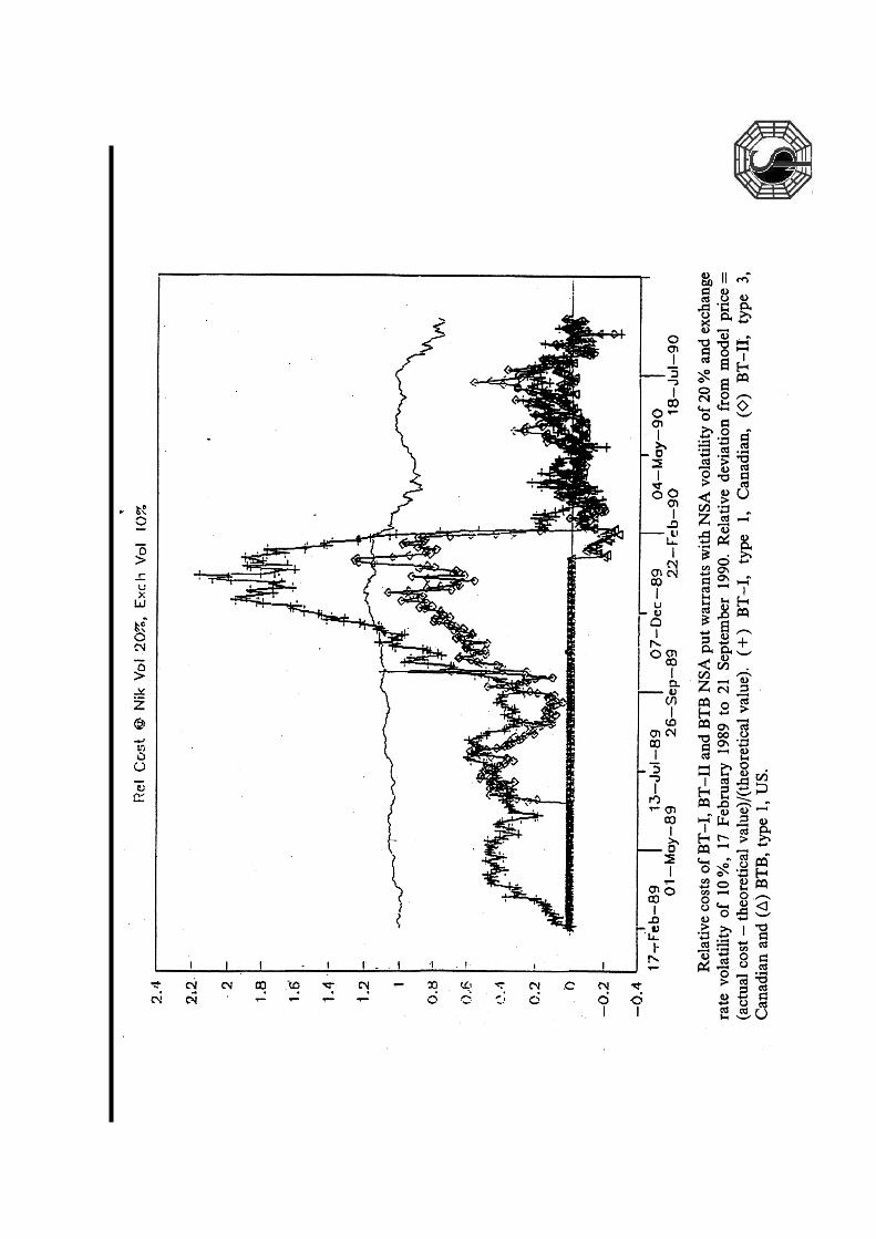
The following figures show the two convergence trades.

Simulation results

is plotted rather than implied volatility since the latter did not exist when there were deep in the money options trading for less than intrinsic as in this market.

Fair value at 20\% NSA volatility and 10\% exchange rate volatility is zero on the graph. At one, the puts are trading for double their fair price.

At the peak, the puts were selling for more than three times their fair price.

• There was a similar inefficiency in the call market where the currency protected options traded for higher than fair prices.

• There was a successful trade here but this was a low volume market.

• This market never took off as investors lost interest when the NSA did not rally. US traders prefered Type II (Salomon's SXZ) denominated in dollars rather than the Paine Webber (PXA) which were in yen.

• The Canadian speculators who overpaid for these put warrants that led to our risk arbitrage made \$500 million Canadian since the NSA's fall was so great.

• The issuers of the puts also did well and hedged their positions with futures in Osaka and Singapore.

• The losers were the holders of Japanese stocks.

• This case example illustrates many of the aspects of hedge fund trading risks. Stochastic programming can be used to help determine appropriate risk-return levels of positions over time.

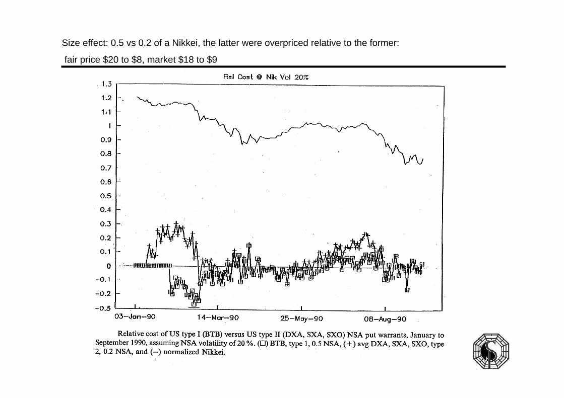
Size effect: 0.5 vs 0.2 of a Nikkei, the latter were overpriced relative to the former:

fair price $20 to $8, market $18 to $9

• PNP gained 15.1% net of fees (which were about 4% given the 20\% profits fee structure) versus 10.2% for the S&P500 and 8.1% for T-bills.

• An initial index of 100 as of November 1, 1969 became, at the end of December 1988, 148,200 in PNP versus 64,500 for the S&P500 and 44,500 for T-bills.

• But what is impressive, and what is a central lesson, is that the risk control using various stochastic optimization procedures led to no years with losses and a high Sharpe ratio which using monthly data approached 3.0.

• In comparison to Keynes, PNP had an easier market to deal with.

• For example, only in 1973, 1974 and 1976 did the S&P500 have negative returns.

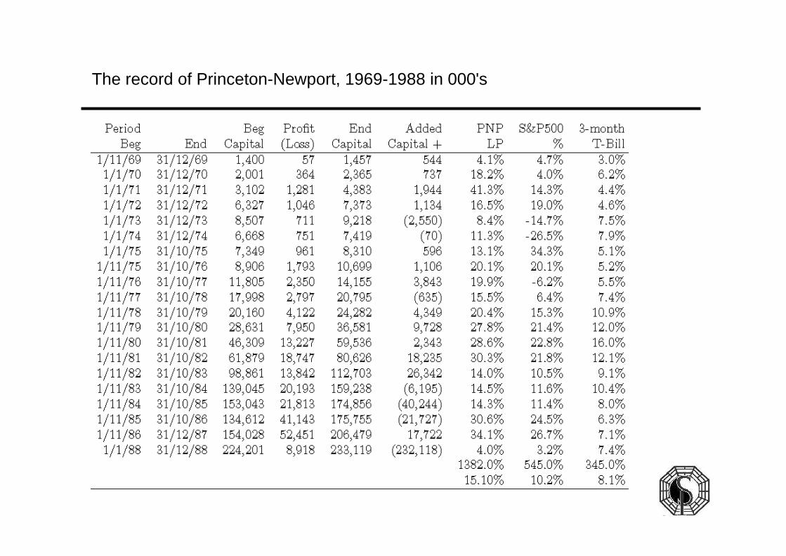
The record of Princeton-Newport, 1969-1988 in 000's

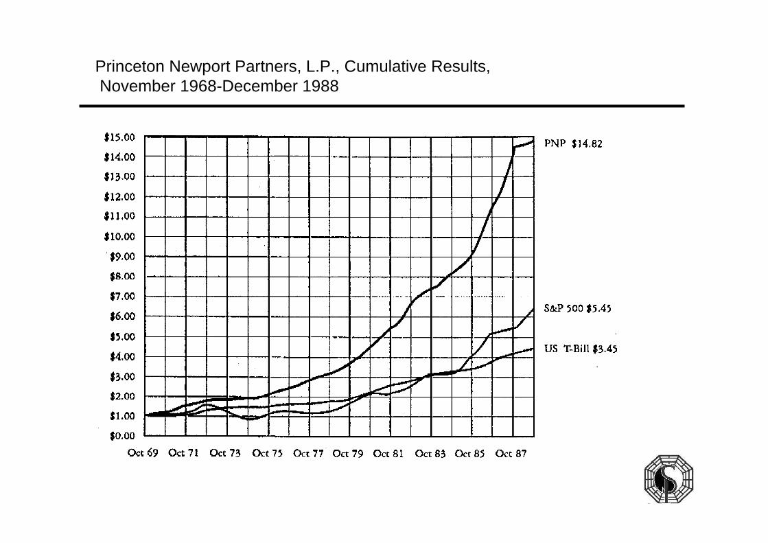
Princeton Newport Partners, L.P., Cumulative Results,November 1968-December 1988

• As a comparison with Keynes and Thorp, the Figure shows the brilliant record of Warren Bufffet's Berkshire Hathaway closed end fund from 1985 to 2000, which is run like a hedge fund with emphasis on value investing, insurance businesses and other ventures.

• Buffett also had a great record from 1977 to 1985, turning 100 into 1429.87 and 65,852.40 in April 2000; and much higher in 2004, coming of a low of about 41,000 in 2000.

• On this same graph are the records of other top hedge funds and related investors such as George Soros' Quantum fund, John Neff's Winsdor mutual fund,

• Julian Robertsons' Tiger Fund and the Ford Foundation.

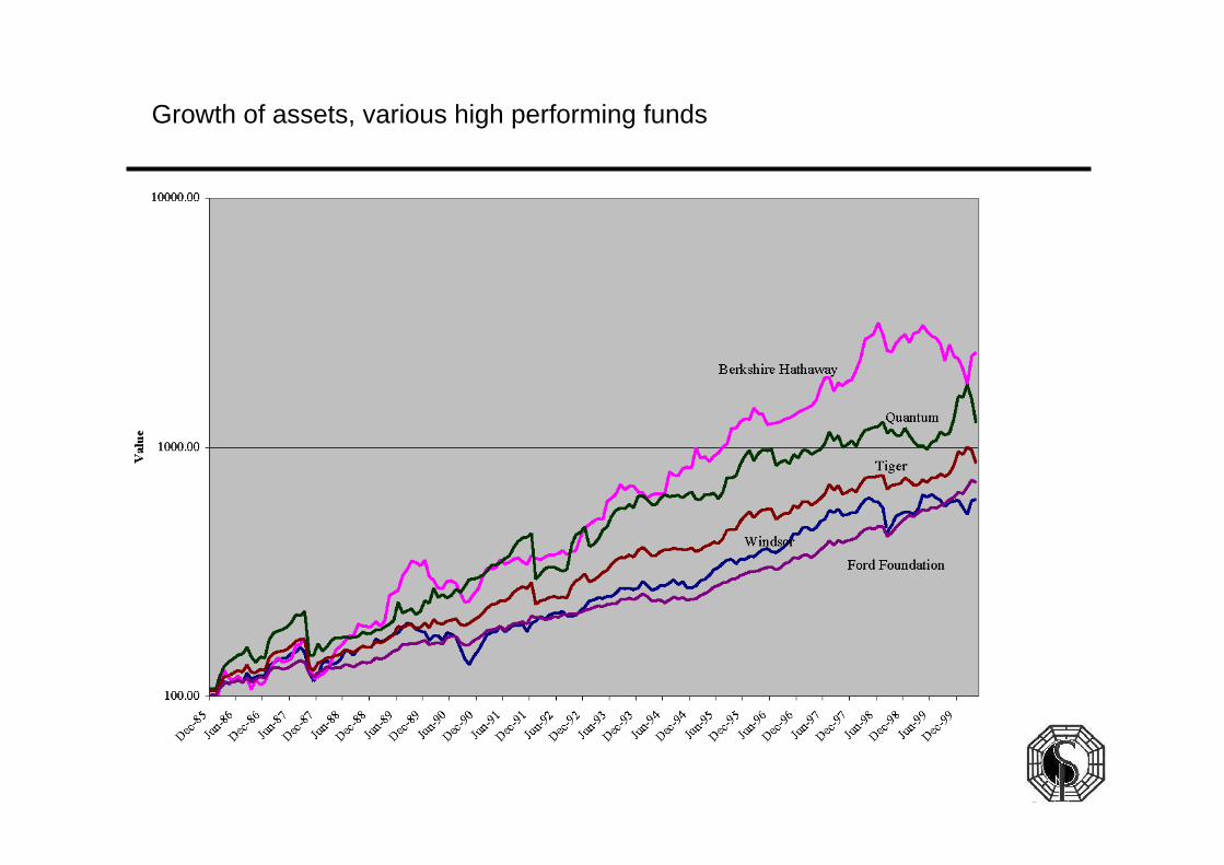
Growth of assets, various high performing funds

• Buffett's Sharpe ratio was 0.786, while the Ford Foundation was 0.818 from January 1980 to March 2000.

• So by the Sharpe measure the Ford Foundation beats Berkshire Hathaway as they have good growth with little variation.

• But much of Berkshire Hathaway's variation is on gains and the total wealth at the horizon is much greater.

• Starting from July 1977 Berkshire Hathaway's Sharpe was 0.850 versus Ford's 0.765 and the S&P was 0.676 with geometric mean returns 32.07% (Buffett), 14.88% (Ford) and 16.71% (S&P500).

• Using the symmetric downside risk measure discussed in Ziemba (2003) provides a fairer evaluation with Berkshire Hathaway dominating as the Figure indicates.

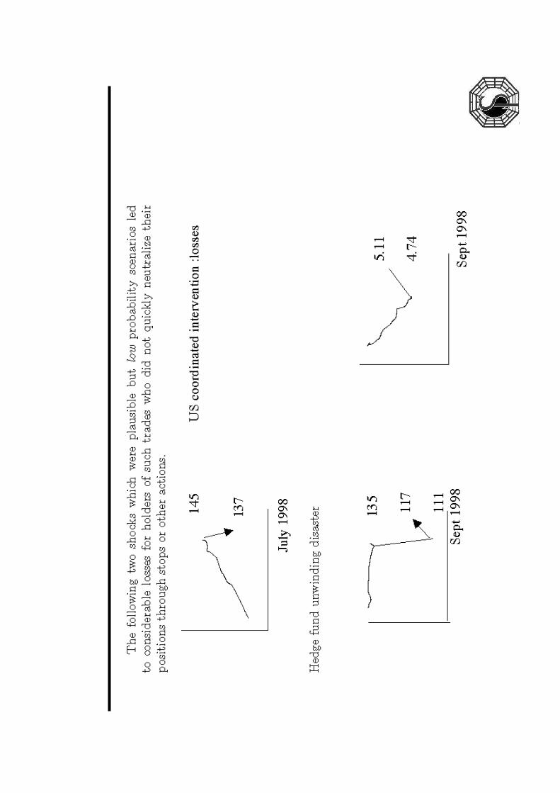
To model this, one needs scenarios on• where are long term interest rates (i) going• where is the ¥/$ exchange rate (y) going

Unforseen factors include• intervention which is always a danger and may or may not be signaled by market

actions; and• hedge funds in trouble may need to unwind other trades to raise cash. This is a

reminder of another danger in today's markets. • One derivative disaster can lead to others because hedge fund traders have

intertwined positions and raising cash to deal with one disaster can create another for someone else.

Hence you must diversify: • One cannot have too much invested in any one strategy and have protective

procedures such as stops to limit losses.• The setting of stop losses is largely an art with very little good theory available

since the problem is very complicated. A useful recent paper is Warburton and Zhang (2002)

• A multiperiod stochastic programming model is useful here.

Comparable to Thorp is the record of Bill Benter, head of the Hong Kong Racing syndicate.

• Factor models to compute expected values of bets, that is probabilities of first, second, third and fourth finishes.

• Similar to picking the best stocks, very complex variables used.

• High transactions costs to overcome with superior models for probabilities and Kelly type optimization over various bets

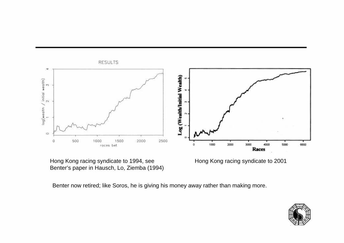
Hong Kong racing syndicate to 2001Hong Kong racing syndicate to 1994, see Benter’s paper in Hausch, Lo, Ziemba (1994)

Benter now retired; like Soros, he is giving his money away rather than making more.

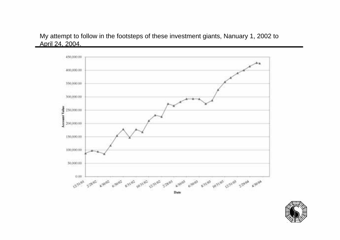
My attempt to follow in the footsteps of these investment giants, Nanuary 1, 2002 to April 24, 2004.

I continue to argue that getting the mean right; and watching our risk control and especially not overbetting are the keys to success. I have done three types of trades (I am small so that's enough for my resources in this futures account):

• hedged currency trades where the key is to get the mean right and devise strategies and positions to capture this;

• security market anomaly trades like the turn-of-the-year effect; and• exploiting systematic biases in the \sp500 futures put and call markets.

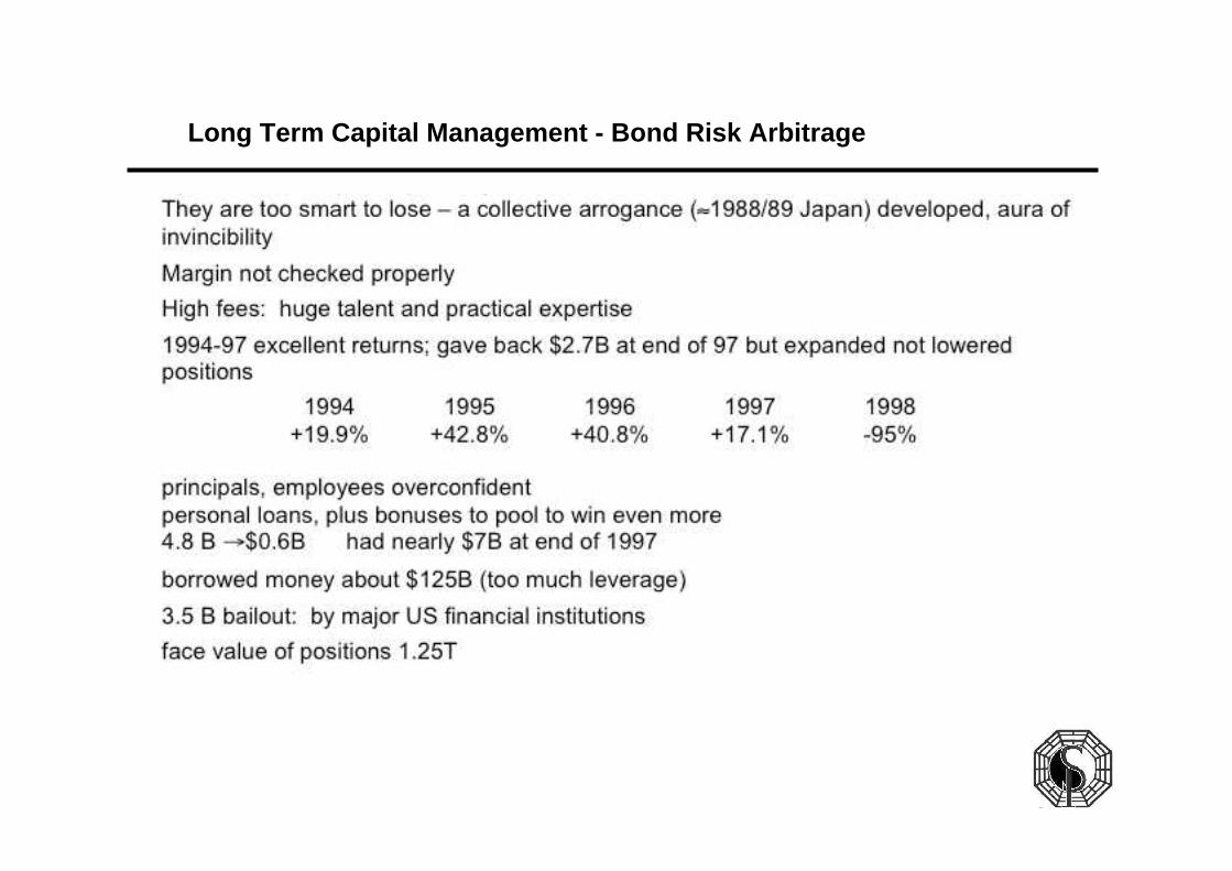
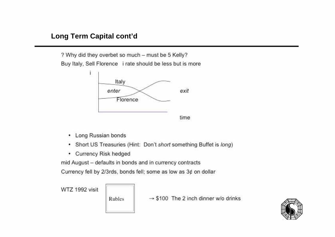
Long Term Capital Management - Bond Risk Arbitrage

Long Term Capital cont’d

Long Term Capital cont’d

Long Term Capital cont’d

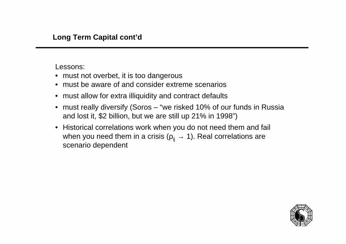
Lessons: • must not overbet, it is too dangerous• must be aware of and consider extreme scenarios

• must allow for extra illiquidity and contract defaults

• must really diversify (Soros – “we risked 10% of our funds in Russia and lost it, $2 billion, but we are still up 21% in 1998”)

• Historical correlations work when you do not need them and fail when you need them in a crisis (ρij → 1). Real correlations are scenario dependent

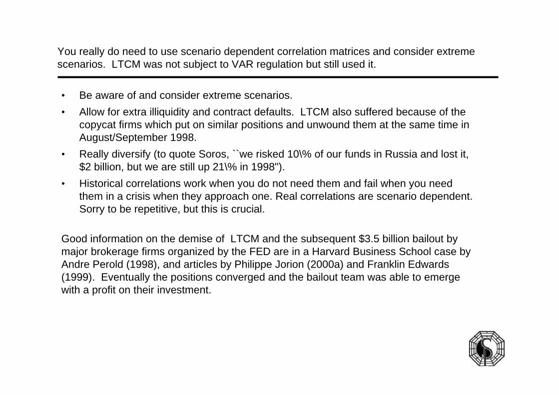
• Be aware of and consider extreme scenarios.

• Allow for extra illiquidity and contract defaults. LTCM also suffered because of the copycat firms which put on similar positions and unwound them at the same time in August/September 1998.

• Really diversify (to quote Soros, ``we risked 10\% of our funds in Russia and lost it, $2 billion, but we are still up 21\% in 1998").

• Historical correlations work when you do not need them and fail when you need them in a crisis when they approach one. Real correlations are scenario dependent. Sorry to be repetitive, but this is crucial.

You really do need to use scenario dependent correlation matrices and consider extreme scenarios. LTCM was not subject to VAR regulation but still used it.

Good information on the demise of LTCM and the subsequent $3.5 billion bailout by major brokerage firms organized by the FED are in a Harvard Business School case by Andre Perold (1998), and articles by Philippe Jorion (2000a) and Franklin Edwards (1999). Eventually the positions converged and the bailout team was able to emerge with a profit on their investment.

• The currency devaluation of some two thirds was no surprise to me.

• In 1992 my family and I were the guests in St. Petersburg of Professor Zari Rachev, an expert in stable and heavy-tail distributions and editor of the first handbook in North Holland's Series on Finance (Rachev, 2003) of which I am the series editor.

• As we arrived I gave him a \$100 bill and he gave me six inches of 25 Ruble notes.

• Our dinner out cost two inches for the four of us; and drinks were extra in hard currency.

• So I am in the Soros camp; make bets in Russia if you have an edge but not risking too much of your wealth.

• The score card according to Dunbar (2000) was a loss of $4.6 billion.

• Emerging market trades such as those similar to my buy Italy, sell Florence lost 430 million.

• Directional, macro trades lost 371 million.

• Equity pairs trading lost 306 million.

• Short long term equity options, long short term equity lost 1.314 billion.

• Fixed income arbitrage lost 1.628 billion.

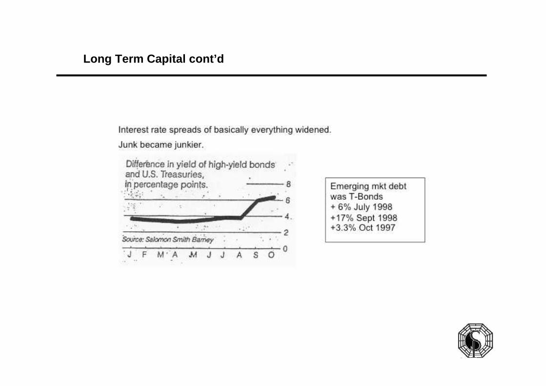
• The bad scenario of investor confidence that led to much higher interest rates for lower quality debt and much higher implied equity volatility had a serious effect on all the trades.

• The long-short equity options trades, largely in the CAC40 and Dax equity indices, were based on a historical volatility of about 15% versus implieds of about 22%.

• Unfortunately, in the bad scenario, the implieds reached 30\% and then 40%.

• With smaller positions, the fund could have waited it out but with such huge levered positions, it could not.

• Equity implieds can reach 70% or higher as Japan's Nikkei did in 1990/1991 and stay there for many months.

Where was the money lost?

The imported crash of October 27 and 28, 1997

• A currency crisis developed in various Asian countries in mid 1997. It started in Thailand and moved all across the region.

• The problem was lack of foreign reserves that occurred because spending and expectations that led to borrowing were too high and Japan, the main driver of these economies, was facing a consumer slowdown so its imports dropped.

• Also loans were denominated in what was then considered a weak currency, the US dollar.

• So that effectively these countries were long yen and short dollars. A large increase in the US currency in yen terms exacerbated the crisis.

• The countries devalued their currencies, interest rates rose and stock prices fell.

• A well-known hedge fund failure in 1997 was Victor Niederhoffer's fund which had an excellent previous record with only modest drawdowns.

• A large long bet on cheap Thai stocks that became cheaper and cheaper turned $120 million into $70 million.

• Buying on dips added to losses. Then the fund created a large short position in out-of-the-money S&P futures index puts.

• A typical position was November 830's trading for about $4-6 at various times around August-September 1997.

• The crisis devastated the small economies of Malaysia, Singapore, Indonesia, etc.

• Finally it spread to Hong Kong.

• There, the currency was pegged to the US dollar at around 7.8.

• The peg was useful for Hong Kong's trade and was to be defended at all costs.

• The weapon used was higher interest rates which almost always lead to a stock market crash but with a lag.

• See the discussion in chapter 3 of my AIMR book (Ziemba, 2003) for the US and Japan and other countries.

• The US S&P500 was not in the danger zone in October 1997 by my models and I presume by others and the trade with Hong Kong and Asia was substantial but only a small part of the US trade. US investors thought that this Asian currency crisis was a small problem because it did not affect Japan very much. In fact, Japan caused a lot of it.

• The week of October 20-25 was a difficult one with the Hang Seng dropping sharply.

• The S&P was also shaky so the November 830 puts were 60 cents on Monday, Tuesday and Wednesday but rose to 1.20 Thursday and 2.40 on Friday.

• The Hang Seng dropped over 20% in a short period including a 10% drop on Friday, October 25.

• The S&P 500 was at 976 way above 830 as of Friday's close.

• A further 5% drop on Monday, October 27 in Hong Kong led to a panic in the \sp500 futures later on Monday in the US.

• The fall was 7% from 976 to 906 which was still considerably above 830.

• On Tuesday morning there was a further fall of 3% to 876 still keeping the 830 puts out of the money.

• The full fall in the S&P500 was then 10%.

• But the volatility exploded and the 830's were in the $16 area.

• Refco called in Niederhoffer's puts mid morning. They took a loss of about $20 million.

• So Niederhoffer's $70 million fund was bankrupt and actually in the red since the large position in these puts and other instruments turned 70 million into minus 20 million.

• The S&P500 bottomed out around the 876 area and moved violently in a narrow range then settled and then moved up by the end of the week right back to the 976 area. So it really was a tempest in a teapot like the cartoon depicts.

• The November 830 puts expired worthless. Investors who were short equity November 830 puts were required to put up so much margin that that forced them to have small positions and they weathered the storm and their $4-$6, while temporarily behind at $16 did eventually go to zero.

• So did the futures puts, but futures shorters are not required to post as much margin so if they did not have adequate margin because they had too many positions. They could have easily been forced to cover at a large loss.

• I argue that futures margins, at least for equity index products, do not fully capture the real risk inherent in these positions. I follow closely the academic studies on risk measures and none of the papers I know deals with this issue properly.

• When in doubt, always bet less. Niederhoffer is back in business having profited by this experience.

• One of my Vancouver neighbors, I learned later, lost $16 million in one account and $4 million in another account. The difference being the time given to cash out and cover the short puts.

• I was in this market also and won in the equity market and lost in futures. It did teach me how much margin you actually need in futures which I use now in such trading which has been very profitable with a few wrinkles to protect oneself that I need to keep confidential.

• One of the naked strategies won 64 out of 65 times from 1987 to September 2002 and seven times since. A hedged strategy had a 45% geometric mean with 60 of 65 winners with the five ruled too risky by a cash, option price danger control measure out of the 70 possible plays in those 17 years and a seven symmetric downside Sharpe, plus seven more winners.

• The lessons for hedge funds are much as with LTCM. Do not overbet, do diversify, watch out for extreme scenarios.

• Even the measure to keep one out of potentially large falls (the 5 of 70 above) did not work in October 1997. That was an imported fear-induced crash not really based on US economics.

• My experience is that most crashes occur when interest rates relative to price earnings ratios are too high. In that case there almost always is a crash, see Ziemba (2003) for the 1987 US, the 1990 Japan, and the US in 2000 are the leading examples as in US in 2001, which predicted the over 20% fall in the S&P500 in 2002.

• Interestingly the measure moved out of the danger zone then in mid 2001 it become even more in the danger zone than in 1999 See Figure. There is more on this in Ziemba (2003).

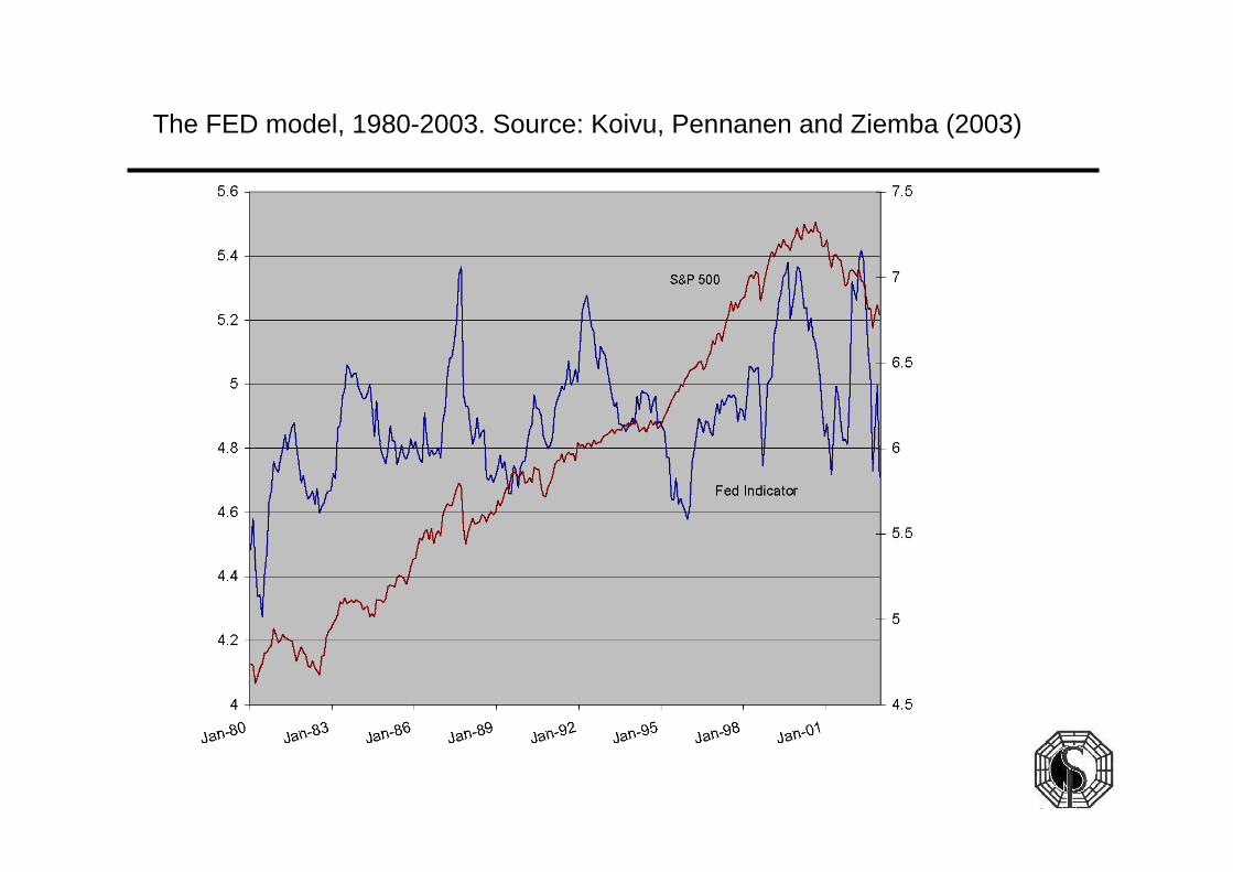
The FED model, 1980-2003. Source: Koivu, Pennanen and Ziemba (2003)

• The idea is when long bond interest rates get too high relative to stock returns as measured by the earnings over price yield method then there almost always is a crash.

• I used a difference method in Ziemba-Schwartz (1991)and results of that are in Ziemba (2003). The graph here uses a ratio or log approach and is equivalent to what is now called the Fed model.

• I started using these measures in 1988 in my study group in Japan at Yamaichi Research. It predicted the 1987 crash; see that on this graph. It also predicted the 1990 Japan crash and I told Yamaichi executives about this in 1989. but they would not listen. Yamaichi went bankrupt in 1995; they would have survived if they had listened to this research.

• They could have paid me a million dollars for an hour’s consulting and still made more than 1000 time profit from the advice. It was more important for them to be nice to my family and me as they were than to listen to the results of a gaijin professor. How could he possibly understand the Japanese stock market? In fact all the economics ideas were there; see Ziemba and Schwartz (1991). I did enjoy these lectures, dinners and golf but being listened to dominates.

• We found for 1948 to 1988 that every time the measure was in the danger zone there was a fall of 10% or more with no misses. In late 1989 the model had the highest reading ever in the danger zone and predicted the January 1990 start of the crash then.

• Back to 1999 in the US. See the measure in the danger zone during 1999 and the subsequent fall in the S&P500 in 2000. Then see the drop in the measure out of the danger zone as prices fell.

• But then in mid 2001, earnings fell more than prices so the measure went back into the danger zone and we had the 22% fall in the S&P in 2002. The measure then moved in 2003 into the buy zone and predicted the rise in the S&P500 we had in 2003.

• No measure is perfect but this measure adds value and tends to keep you out of extreme trouble.

• But a mini crash caused by some extraneous event can occur any time. So to protect oneself positions must never be too large. Koliman (1998) and Crouhy, Galai and Mark in Gibson's (2000) book on model risk discusses this. Their analysis there suggests it's a violation of lognormality which I agree it was.

• Increased implied volatility premiums caused the huge losses of those who had to cash out because of margin calls because they had too many positions.

The top ten points to remember about the stochastic programming approach to asset liability and wealth management.

Point 1 - Means are by far the most important part of the distribution of returns – especially the direction.

→ You must estimate future means well or you can travel very fast in the wrong direction and that usually leads to losses or underperformance.

Point 2 - Mean variance models are useful as a basic guideline when you are in an assets only situation. Professionals adjust means using mean-reversion, James-Stein or truncated estimators and constrain output weights.

→ Do not change asset positions unless the advantage of the change is significant. Do not use mean variance analysis with liabilities and other major market imperfections except as a first test analysis.

Point 3 - Trouble arises when one overbets and a bad scenario occurs

→ You must not overbet when there is any possibility of a bad scenario occurring unless the bet is protected by some type of hedge or stop-loss.

Point 4 - Trouble is exacerbated when the expected diversification does not hold in the scenario that occurs

→ You must use scenario dependent correlation matrices because simulations around historical correlation matrices are inadequate for extreme scenarios.

Point 5 - When there is a large decline in the stock market, the positivecorrelation between stocks and bond fails and they become negatively correlated

→ When the mean of the stock market is negative, bonds are more attractive as is cash.

Point 6 - Stochastic programming scenario based models are useful when one wants to look at aggregate overall decisions with liabilities, liquidity, taxes, policy, legal and other constraints and have targets and goals you want to achieve.

→ It pays to make a complex stochastic programming model when a lot is at stake and the essential problem has many complications.

Point 7 - Other approaches, continuous time finance, decision rule based SP, control theory, etc are useful for problem insights and theoretical results. But in actual use, they may lead to disaster unless modified. The Black-Scholes theory says you can hedge perfectly with log normal assets and this can lead to overbetting.

But fat tails and jumps arise frequently and can occur without warning. The S&P opened limit down –60 points or 6% when trading resumed after Sept 11, 2001 and it fell 14% that week.

→ Be careful of the assumptions, including implicit ones, of theoretical models. Use the results with caution no matter how complex and elegant the math or how smart or famous the author. Remember you have to be very smart to lose millions and even smarter to lose billions.

Point 8 - Do not be concerned with getting all the scenarios exactly right when using stochastic programming models.

You cannot do this and it does not matter that much anyway.

Rather worry that you have the problems’ periods laid out reasonably and the scenarios basically cover the means, the tails and the chance of what could happen. If the current situation has never occurred before, use one that is similar to add scenarios.

For a crisis in Brazil, use Russian crisis data, for example. The results of the SP will give you good advice when times are normal and keep you out of severe trouble when times are bad.

Those using SP models may lose 5-10-15% but they will not lose 50-70-95% like some investors and hedge funds.

→ If the scenarios are more or less accurate and the problem elements reasonably modeled, the SP will give good advice.

You may slightly outperform in normal markets but you will greatly outperform in bad markets when other approaches may blow up.

Point 9 - SP models for ALM were very expensive in the 1980s and early 1990s but are not very expensive now. Vancouver analysts using a large linear programming model to plan lumber operations at MacMillan Blodel used to fly to San Francisco to use a large computer which would run all day to run the model once. Now models of this complexity would take only seconds on an inexpensive desk top computer.

→ Advances in computing power and modeling expertise have made SPmodeling not very expensive.

Such models are still complex and require approximately six months to develop and test, costing a couple hundred thousand dollars. A small team can now make a model for a complex organization quite quickly at fairly low cost compared to what is at stake.

Point 10 - Eventually as there are more disasters and more successful SP models are built and used, they will become popular.

→ The ultimate goal is to have them in regulations like VaR. While VaR does more good than harm, it's safety is questionable in many applications. C-VaR is an improvement but for most people and organizations the non-attainment of goals is more than proportional, that is, convex in the non-attainment.